Eigenfunction Families and Solution Bounds for Multiplicatively Advanced Differential Equations

Abstract

A family of Schwartz functions $\mathcal{W}(t)$ are interpreted as eigensolutions of MADEs in the sense that ${\mathcal{W}}^{(\delta )}(t)=E\mathcal{W}(q^{\gamma }t)$ where the eigenvalue $E\in \mathbb{R}$ is independent of the advancing parameter $q>1$. The parameters $\delta ,\gamma \in \mathbb{N}$ are characteristics of the MADE. Some issues, which are related to corresponding q-advanced PDEs, are also explored. In the limit that $q\to 1^{+}$ we show convergence of MADE eigenfunctions to solutions of ODEs, which involve only simple exponentials and trigonometric functions. The limit eigenfunctions ($q=1^{+}$) are not Schwartz, thus convergence is only uniform in $t\in \mathbb{R}$ on compact sets. An asymptotic analysis is provided for MADEs which indicates how to extend solutions in a neighborhood of the origin $t=0$. Finally, an expanded table of Fourier transforms is provided that includes Schwartz solutions to MADEs.

1. Introduction

The introduction of a relaxing parameter $q>1$ in differential equations was found to provide stability properties for their corresponding solutions. This is a phenomenon well-known in numerical analysis where if the Ordinary Differential Equation (ODE)

$$y^{\prime }(t)=f\left(t,y(t)\right),y(t_0)=y_0,$$

is stiff then one can try to use the backward Euler method to obtain the sequence ${\left\{\langle t_n,y_n\rangle \right\}}_{n=0}^{\infty }$ by first considering the algebraic equations

$$t_{n+1}=t_n+\Delta t,y_{n+1}=y_n+f(t_{n+1},y_{n+1})·\Delta t,$$

for small time-steps $\Delta t>0$. If one can obtain $y_{n+1}$ explicitly in terms of $y_n$ then the iteration scheme often converges much faster, and for longer time intervals, than that provided by the forward Euler method [1], p. 349. That such a principle holds for ODEs as $\Delta t\to 0^{+}$ was established through the study of Multiplicatively Advanced Differential Equations (MADEs) as $q\to 1^{+}$, and will be discussed further in this article. Part of our analysis of stability will require obtaining uniform apriori bounds. This will be achieved in a somewhat general setting, and the consequences will be presented in the form of examples of advanced differential equations.

1.1. Solutions of MADEs as Eigenfunctions

In [2] solutions to equations of the form

$$y^{\prime }(t)=ay(qt)+by(t),y(0)=1\mathrm{or}0(\mathrm{wlog}),$$

(1)

were studied for $q>1$, $a\in \mathbb{C}$, $b\in \mathbb{R}$ and $t\ge 0$. In the case that $b=0$, with $y(0)=0$, solutions $y(t)$ are referred to as eigenfunctions since $y(t)\to 0$ as $t\to \infty$. Specific asymptotic properties of solutions were obtained in Theorem 10 of [3]. Here we only consider the case that $b=0$ and $a\in \mathbb{R}$, however the derivatives may be of higher (integer) order than in Equation (1). In addition, we extend solutions of these equations to all $t\in \mathbb{R}$ so that the eigen equation, referred to as an eigen-MADE, has a solution $y(t)\in \mathcal{S}(\mathbb{R})$ the Schwartz space of infinitely differentiable functions, with derivatives that decay faster than reciprocal polynomials (as defined in [4] section V.3). An asymptotic theory near $t=0$ can be developed indicating that an extension to $t<0$ is quite natural. In this way the special functions that we study are eigenfunctions in ${\mathcal{L}}^2(\mathbb{R})$, although not in the traditional, local ($q=1$) sense. The significance of these functions will be demonstrated by examples, and convergence to familiar functions is obtained on compact subsets of $\mathbb{R}$, as $q\to 1^{+}$.

1.2. Brief Overview

The study of multiply advanced differential equations falls within the area of functional differential equations, as is studied for instance in Fox, et al. [2], Kato, et al. [3] and Dung [5]. There is also significant overlap with the area of q-difference differential equations, where the multiplicative advancement $y(t)\to y(qt)$ is referred to as a dilation and is denoted ${\sigma }_q(y(t))=y(qt)$. There is a rich and active study within the area of q-difference differential equations with dilations involving $q>1$. These are highlighted by works of: L. Di Vizio [6,7,8]; C. Hardouin [7]; T. Dreyfus [9,10]; A. Lastra [10,11,12,13,14,15,16,17,18,19]; S. Malek [10,11,12,13,14,15,16,17,18,19,20,21,22]; J. Sanz [17,18,19]; H. Tahara [23]; and C. Zhang [8,24]; along with further references by these researchers and others. Often these studies in q-difference differential equations overlap with the area of Gevrey asymptotics.

In the current work we continue by focusing on global solutions of a MADE on $\mathbb{R}$. In particular, we discuss several techniques for starting with a given global solution to an original MADE and then generating solutions of new related MADEs. This theme will be developed as follows: In Section 2, a known MADE solution first introduced in [25], namely ${}_{q}Cos(t)$, is used to produce a simple related solution ${\tilde{C}}_q(t)={}_{q}Cos(t/\sqrt{q})$ which is an eigensolution of a MADE in the sense of the Abstract. In turn, ${\tilde{C}}_q(t)$ is then used to obtain a new q-advanced Airy function $Aiq(t)$ satisfying a MADE analogue of the Airy differential equation. Then $Aiq(t)$ itself is used along with convolution to generate families of functions ${\varphi }_q(x,t)$ solving a q-advanced PDE.

In Section 3, a family of MADE solutions, under convolution and auto-correlation, are seen to produce related solutions of new MADEs. Furthermore, the least-element method in Poincare asymptotics is deployed to find natural extensions to related MADE solutions on the negative real line. A theory of asymptotic extensions to $t<0$ is developed to clarify the notion that solutions to MADEs behave smoothly in a neigborhood of the origin. We also give conditions that ensures a natural extension to all of $\mathbb{R}$, as is needed to even consider a Fourier transform. An investigation of the inhomogeneous MADEs that these solve is begun.

In Section 4 we focus on considering solutions of MADEs as perturbations of classical solutions, and, mirroring a more direct convergence proof in Section 2, we exhibit MADE solutions which converge to a classical solution of a damped-oscillation equation—the convergence being uniform on compact subsets of $[0,\infty )$.

In Section 5, we return to the topics of convolution and auto-correlation to observe their impact when applied to MADE solutions. In this paper, we will discuss convolutions, correlations, and Fourier transforms for MADEs.

A table of Fourier transforms of global MADE solutions under study here is provided in Section 6. These will be solutions of new MADEs, for which we obtain new elements in a table of Fourier transforms. This new table mimics what is often done for Laplace transforms, in the study of linear constant coefficient ODEs.

In various theories of differential equations, convolutions provide a useful tool since general solutions can be determined from fundamental solutions, as demonstrated here in Equation (33). This is one motivation for obtaining solutions to homogenous equations, as appears in Proposition 2.

2. A Normalized Cosine Example and Extensions

From [25], consider the following Schwartz functions, for $q>1$ and all $t\in \mathbb{R}$,

$$\begin{array}{cc}\hfill & {}_{q}Cos(t)\equiv N_q\sum _{k=-\infty }^{\infty }\frac{{(-1)}^k}{q^{k^2}}·exp(-q^k|t|)\hfill \end{array}$$

(2)

$$\begin{array}{cc}\hfill & {}_{q}Sin(t)\equiv sign(t)N_q\sum _{k=-\infty }^{\infty }\frac{{(-1)}^k}{q^{k(k-1)}}exp(-q^k|t|),\hfill \end{array}$$

(3)

where

$$\frac{1}{N_q}\equiv \sum _{k=-\infty }^{\infty }\frac{{(-1)}^k}{q^{k^2}}.$$

(4)

Next define

$${\tilde{C}}_q(t)\equiv {}_{q}Cos\left(\frac{t}{\sqrt{q}}\right)=N_q\sum _{k=-\infty }^{\infty }\frac{{(-1)}^k}{q^{k^2}}·exp\left(\frac{-q^k|t|}{\sqrt{q}}\right).$$

(5)

There are several properties that we note. In particular, the function ${\tilde{C}}_q(t)$ is normalized, in that the uniform bound ${\parallel {\tilde{C}}_q\parallel }_{\infty }=1$ holds, after some delicate work performed in [25], for each $q>1$. It also solves the following eigen-MADE for all $t\in \mathbb{R}$ and each $q>1$,

$$\frac{d^2{\tilde{C}}_q(t)}{d{t}^2}=-{\tilde{C}}_q(qt),{\tilde{C}}_q(0)=1,{\tilde{C}}_q^{\prime }(0)=0.$$

(6)

From (6) we see that ${\tilde{C}}_q(t)$ satisfies an eigen-MADE in the sense of the Abstract, with $E=-1$ independently of the advancing parameter $q>1$. Note that ${{}_{q}Cos}^{″}(t)=-q{}_{q}Cos(qt)$ (as recorded in (10) below) does not have an eigenvalue $(-q)$ independent of q, thus we rely on ${\tilde{C}}_q(t)$ as the appropriate eigen-MADE solution.

Since ${\tilde{C}}_q(t)$ is not only ${\mathcal{C}}^{\infty }$ and bounded, but in fact Schwartz, we can obtain its Fourier transform, an operation defined for any $f\in {\mathcal{L}}^1(\mathbb{R})$, as

$$\widehat{f}(\omega )=\mathcal{F}[f(t)](\omega )\equiv \frac{1}{\sqrt{2\pi }}{\int }_{-\infty }^{\infty }{e}^{-i\omega t}·f(t)dt.$$

In [25] it was found that

$$\mathcal{F}[{\tilde{C}}_q(t)](\omega )=\frac{2{({\mu }_{q^2})}^3{N}_q}{\sqrt{2\pi }}·\frac{1}{\theta (q^2;q{\omega }^2)},$$

(7)

where $N_q$ was defined in Equation (4) above, and the other normalizing constant is

$${\mu }_q\equiv \prod _{n=1}^{\infty }\left(1-\frac{1}{q^n}\right).$$

To express the Fourier transform of linear, homogeneous MADEs, we found multiple uses of the Jacobi theta function

$$\theta (q;u)\equiv \sum _{n=-\infty }^{\infty }\frac{u^n}{q^{n(n-1)/2}}={\mu }_q·(1+u)·\prod _{n=1}^{\infty }\left(1+\frac{u}{q^n}\right)\left(1+\frac{1}{u{q}^n}\right),$$

(8)

which allows the association that $N_q=\theta (q^2;-1/q)$, and which ensures that $N_q\ne 0$ for all $q>1$, due to the product formula. It will be of significance to note that the reciprocal $1/\theta (q;u)$, for $u\ge 0$, is Schwartz when extended to be identically 0 for $u<0$. Critical algebraic properties that we use are

$$\theta (q;q^{p}u)=q^{p(p+1)/2}{u}^p·\theta (q;u),\forall p\in \mathbb{Z},u\in {\mathbb{C}}^{\ast },\mathrm{and}v·\theta (q;1/v)=\theta (q;v),\forall v\in {\mathbb{C}}^{\ast }.$$

(9)

A consequence is that the only zeros of $\theta (q;u)$ are for $u=-q^p$ for all $p\in \mathbb{Z}$. This is obvious from the product definition of $\theta (q;u)$ in Equation (8).

2.1. Uniform Convergence

Using Taylor series methods as an approach paralleling that in [25] we show:

Proposition 1.

On any compact subset of $\mathbb{R}$, ${\tilde{C}}_q(t)$ approaches $cos(t)$ uniformly as $q\to 1^{+}$.

Proof. 

A given compact set is contained in an interval $[-\rho ,\rho ]$ for $\rho$ sufficiently large, so it suffices to prove the theorem on $[-\rho ,\rho ]$.

First, recall the following results shown in [25]

$$\begin{array}{cc}\hfill {}_{q}Cos(0)=1& {}_{q}Sin(0)=0\hfill \\ \hfill {}_{q}Co{s}^{\prime }(t)={-}_{q}Sin(t)& {}_{q}Si{n}^{\prime }(t)=q{}_{q}Cos(qt)\hfill \\ \hfill {}_{q}Co{s}^{″}(t)=-q{}_{q}Cos(qt)& {}_{q}Si{n}^{″}(t)=-q^2{}_{q}Sin(qt).\hfill \end{array}$$

(10)

From these, by induction on the even order derivatives of ${}_{q}Cos(t)$, we obtain the higher order derivatives

$${}_{q}Co{s}^{(2L)}(t)={(-1)}^L{q}^{L^2}{}_{q}Cos(q^{L}t),$$

(11)

and

$${}_{q}Co{s}^{(2L+1)}(t)={[{(-1)}^L{q}^{L^2}{}_{q}Cos(q^{L}t)]}^{\prime }={(-1)}^{L+1}{q}^{L^2+L}{}_{q}Sin(q^{L}t).$$

(12)

We infer all derivatives of ${\tilde{C}}_q(t)$ via

$$\begin{array}{}\mathrm{(13)}& \hfill {\tilde{C}}_q^{(2L)}(t)& =& {{[}_{q}Cos(t/\sqrt{q})]}^{(2L)}={(-1)}^L{q}^{L^2}{}_{q}Cos(q^{L}t/\sqrt{q}){(1/\sqrt{q})}^{(2L)}\hfill \mathrm{(14)}& & =& {(-1)}^L{q}^{L^2-L}{}_{q}Cos(q^{L}t/\sqrt{q})={(-1)}^L{q}^{L^2-L}{\tilde{C}}_q(q^{L}t),\hfill \end{array}$$

and

$${\tilde{C}}_q^{(2L+1)}(t)={[{(-1)}^L{q}^{L^2-L}{}_{q}Cos(q^{L}t/\sqrt{q})]}^{\prime }={(-1)}^{L+1}{q}^{L^2-1/2}{}_{q}Sin(q^{L}t/\sqrt{q}).$$

(15)

Evaluating the derivatives of ${\tilde{C}}_q(t)$ at $t=0$ yields

$${\tilde{C}}_q^{(2L)}(0)={(-1)}^L{q}^{L^2-L}\mathrm{and}{\tilde{C}}_q^{(2L+1)}(0)=0$$

(16)

for all $L\ge 0$.

Next computing $P_{2N+1}[{\tilde{C}}_q](t)$, the $2N+1$ degree Taylor polynomial for ${\tilde{C}}_q(t)$ expanded about $t=0$, gives

$$\begin{array}{c}\hfill P_{2N+1}[{\tilde{C}}_q](t)=\sum _{p=0}^{2N+1}\frac{{\tilde{C}}_q^{(p)}(0)}{p!}{t}^p=\sum _{L=0}^N\frac{{(-1)}^L{q}^{L^2-L}}{(2L)!}{t}^{2L},\end{array}$$

(17)

with remainder term

$$R_{2N+1}[{\tilde{C}}_q](t)=\frac{{\tilde{C}}_q^{(2N+2)}(\xi )t^{2N+2}}{(2N+2)!}=\frac{{(-1)}^{N+1}{q}^{{(N+1)}^2-(N+1)}{\tilde{C}}_q(q^{N+1}\xi )t^{2N+2}}{(2N+2)!},$$

(18)

for appropriate $\xi$ between 0 and t. Using the sup norm ${\parallel {\tilde{C}}_q\parallel }_{\infty }={\parallel {}_{q}Cos\parallel }_{\infty }={}_{q}Cos(0)=1$, along with the fact that $|t|\le \rho$, to bound from above, we obtain

$$\begin{array}{c}\hfill |R_{2N+1}[{\tilde{C}}_q](t)|=\frac{q^{N^2+N}|{\tilde{C}}_q(q^{N+1}\xi ){||t|}^{2N+2}}{(2N+2)!}\le \frac{q^{N^2+N}{\rho }^{2N+2}}{(2N+2)!}.\end{array}$$

Let $P_{2N+1}[cos](t)$ and $R_{2N+1}[cos](t)$ denote the $2N+1$ degree Taylor polynomial and remainder terms for $cos(t)$ respectively. Then, for each $N\ge 1$ and each t with $|t|\le \rho$, one has

$$\begin{array}{}\mathrm{(19)}& \hfill & \left|{\tilde{C}}_q(t)-cos(t)\right|\hfill & \le & \left|{\tilde{C}}_q(t)-P_{2N+1}[{\tilde{C}}_q](t)\right|+\left|P_{2N+1}[{\tilde{C}}_q](t)-P_{2N+1}[cos](t)\right|+\left|P_{2N+1}[cos](t)-cos(t)\right|\hfill & \le & \left|R_{2N+1}[{\tilde{C}}_q](t)\right|+\left|\sum _{L=0}^N\frac{{(-1)}^L{q}^{L^2-L}}{(2L)!}{t}^{2L}-\sum _{L=0}^N\frac{{(-1)}^L}{(2L)!}{t}^{2L}\right|+\left|R_{2N+1}[cos](t)\right|\hfill & \le & \frac{q^{N^2+N}{\rho }^{2N+2}}{(2N+2)!}+\left(q^{N^2-N}-1\right)\sum _{L=0}^N\frac{{\rho }^{2L}}{(2L)!}+\frac{{\rho }^{2N+2}}{(2N+2)!}\hfill \mathrm{(20)}& \le & \frac{q^{N^2+N}{\rho }^{2N+2}}{(2N+2)!}+\left(q^{N^2-N}-1\right){\mathrm{e}}^{\rho }+\frac{{\rho }^{2N+2}}{(2N+2)!}.\hfill \end{array}$$

Now, given any $ϵ>0$ choose $N_0\ge 1$ such that ${\rho }^{2N_0+2}/(2N_0+2)!<ϵ/3$. Then one has $1<ϵ(2N_0+2)!/[3{\rho }^{2N_0+2}]$. Next choose $q_0>1$ with $1<q_0^{N_0^2+N_0}<ϵ(2N_0+2)!/[3{\rho }^{2N_0+2}]$. Then for all $1<q<q_0$ one has

$$0<\frac{q^{N_0^2+N_0}{\rho }^{2N_0+2}}{(2N_0+2)!}<\frac{q_0^{N_0^2+N_0}{\rho }^{2N_0+2}}{(2N_0+2)!}<\frac{ϵ}{3}\mathrm{and}0<\frac{{\rho }^{2N_0+2}}{(2N_0+2)!}<\frac{ϵ}{3}.$$

(21)

Next choose $q_1>1$ such that $q_1^{N_0^2-N_0}-1<ϵ/[3{\mathrm{e}}^{\rho }]$. Then for all $1<q<q_1$ one has

$$0<\left(q^{N_0^2-N_0}-1\right){\mathrm{e}}^{\rho }<\left(q_1^{N_0^2-N_0}-1\right){\mathrm{e}}^{\rho }<\frac{ϵ}{3}.$$

(22)

For the given $ϵ$, set $N=N_0$ in (19) and (20). Then for $|t|\le \rho$ and all $1<q<min\{q_0,q_1\}$, applying the bounds (21) and (22) to (20) gives

$$\left|{\tilde{C}}_q(t)-cos(t)\right|<\frac{ϵ}{3}+\frac{ϵ}{3}+\frac{ϵ}{3}=ϵ,$$

(23)

verifying uniform convergence of ${\tilde{C}}_q(t)$ to $cos(t)$ on $[-\rho ,\rho ]$ as $q\to 1^{+}$. □

Remark 1.

Note that, alternatively, one can express Proposition 1 as

$$(\forall \mathcal{I}\subset \subset \mathbb{R}\mathrm{compact})\Rightarrow \underset{q\to 1^{+}}{lim}sup\{|{\tilde{C}}_q(t)-cos(t)|:t\in \mathcal{I}\}=0$$

(24)

A similar convergence proof is given in Section 4, with details related to the novelty of the result.

2.2. Application to PDE Example

We are now in a position to obtain q-versions of various equations using ${\tilde{C}}_q(t)$ as a building block for relaxing equations. For example, define the Airy function (see page 570 in [26])

$$Ai(t)\equiv \frac{1}{\pi }{\int }_0^{\infty }cos\left(\frac{u^3}{3}+u·t\right)du,t\in \mathbb{R}.$$

Some properties of this ${\mathcal{C}}^{\infty }(\mathbb{R})$ function are that $Ai(t)\to 0$ as $|t|\to \infty$, and $Ai(0)>0$. We now show:

Proposition 2.

The q-advanced Airy function is defined here to be

$$Aiq(t)\equiv \frac{1}{\pi }{\int }_0^{\infty }{\tilde{C}}_q\left(\frac{u^3}{3}+u·t\right)du,t\in \mathbb{R},$$

(25)

for $q>1$. The functions $Ai(t)$ and $Aiq(t)$ satisfy the homogeneous ODE and MADE

$$A{i}^{″}(t)-t·Ai(t)=0,Ai{q}^{″}(t)-q^{-1/3}t·Aiq\left(q^{2/3}t\right)=0,$$

(26)

respectively, for $t\ge 0$. Basic properties of $Aiq(t)$ for $q>1$, are that $Aiq(t)$ is Schwartz with $Aiq(0)>0$. Furthermore, for each $T>0$, $ϵ>0$, and $R>T$ sufficiently large, $\exists q(ϵ,T,R)>1$ so that

$$sup\left\{\left|Ai(t)-Aiq(t)\right|:|t|\le T,1<q<q(ϵ,T,R)\right\}<ϵ.$$

(27)

In other words, $Aiq(t)\to Ai(t)$ uniformly for t in compact subsets of $\mathbb{R}$, as $q\to 1^{+}$.

Remark 2.

Verifying convergence in Equation (27) may seem rather straight forward, due to the uniform convergence of ${\tilde{C}}_q(t)$ to $cos(t)$ on compact sets. However, we need to use a careful $ϵ/3$ argument, as demonstrated here.

Proof. 

That $Aiq(t)$ is Schwartz follows from the same for ${\tilde{C}}_q(t)$, whereas the property $Aiq(0)>0$ requires a manipulation of theta functions, and is shown in Appendix A. We start with the second equation in (26) since the first equation is known to hold [26]. First define the function

$${\tilde{S}}_q(t)\equiv {\int }_0^t{\tilde{C}}_q(s)ds,\mathrm{so}\mathrm{that}{\tilde{S}}_q(0)=0,{\tilde{S}}_q(\pm \infty )=0.$$

Now compute, using $v=q(u^3/3+ut)$, and $w=q^{1/3}u$, for $t\ge 0$,

$$\begin{array}{ccc}\hfill Ai{q}^{″}(t)& =& \frac{1}{\pi }{\int }_0^{\infty }-u^2{\tilde{C}}_q\left(q·\left(\frac{u^3}{3}+u·t\right)\right)du\hfill \\ \hfill & =& \frac{-1}{q\pi }{\int }_0^{\infty }q(u^2+t)·{\tilde{C}}_q\left(q·(\frac{u^3}{3}+u·t)\right)du+\frac{t}{\pi }{\int }_0^{\infty }{\tilde{C}}_q\left(q·(\frac{u^3}{3}+u·t)\right)du\hfill \\ \hfill & =& \frac{-1}{q\pi }{\int }_0^{\infty }\frac{d{\tilde{S}}_q\left(v\right)}{dv}dv+\frac{t}{\pi }{\int }_0^{\infty }{\tilde{C}}_q\left(\frac{w^3}{3}+w·q^{2/3}t\right)(dw/q^{1/3})\hfill \\ \hfill & =& (-{\tilde{S}}_q(\infty )+{\tilde{S}}_q(0))/(q\pi )+q^{-1/3}t·Aiq\left(q^{2/3}t\right).\hfill \end{array}$$

(28)

Next, to show convergence, consider any $ϵ>0$ and, without loss of generality, fix $T>1$. Let t be in the interval $|t|\le T$. Then, for any $R>T$, using integration by parts and boundedness of the sine function, we can write

$$\begin{array}{ccc}\hfill Ai(t)-\frac{1}{\pi }{\int }_0^{R}cos\left(\frac{u^3}{3}+u·t\right)du& =& \frac{1}{\pi }{\int }_R^{\infty }\frac{1}{u^2+t}·\frac{d}{du}sin\left(\frac{u^3}{3}+u·t\right)du\hfill \\ \hfill & =& \frac{-sin\left(\frac{R^3}{3}+R·t\right)}{\pi (R^2+t)}-\frac{1}{\pi }{\int }_R^{\infty }\frac{-2u}{{(u^2+t)}^2}·sin\left(\frac{u^3}{3}+u·t\right)du\hfill \end{array}$$

(29)

Thus, for all $|t|\le T$ we can easily find $R>T$ sufficiently large so that

$$\left|Ai(t)-\frac{1}{\pi }{\int }_0^{R}cos\left(\frac{u^3}{3}+u·t\right)du\right|\le \frac{2}{\pi ·(R^2-T)}.$$

(30)

The bound in Equation (30) also holds if $Ai(t)$ is replaced with $Aiq(t)$ since $|{\tilde{C}}_q(t)|\le 1$ and $|{\tilde{S}}_q(t)|\le 1$ for all $q>1$. Now, fix $R>0$ sufficiently large so that the bounds in (30), and also (30) with cos replaced by ${\tilde{C}}_q$, are less than $ϵ/3$. It is essential to note that this value of R is independent of $q>1$.

Finally, for each $t\in \mathbb{R}$, define the function

$$V_t(u)\equiv \frac{u^3}{3}+ut,\mathrm{so}\mathrm{that}{V}_t\left([0,R]\right)=\left\{\begin{array}{c}[0,R^3/3+Rt],t\ge 0\hfill \\ \left[-{2|t|}^{3/2}/3,max\{0,R^3/3+Rt\}\right],t<0\hfill \end{array}\right..$$

The union of these $V_t([0,R])$ over $t\in [0,R]$, is the interval $I\equiv [-2T^{3/2}/3,R^3/3+RT]$. From the uniform convergence in Equation (24) we can choose $q(ϵ,T,R)>1$ so that

$$|cos\left(V_t(u)\right)-{\tilde{C}}_q\left(V_t(u)\right)|<\frac{\pi ϵ}{3·R},$$

(31)

for $|t|\le T$, $|u|\le R$, and $1<q<q(ϵ,T,R)$. This is now sufficient to verify the expression in Equation (27). □

2.3. A q-Advanced PDE Example

The argument in the proof of Proposition 2 shows that knowledge of one MADE can help to generate and study other MADEs. In fact, this extends to Partial Differential Equations (PDEs). For example, consider the linear constant-coefficient Airy PDE [27]

$${\partial }_t\varphi (x,t)=a{\partial }_x^3\varphi (x,t),\varphi (x,0)=f(x),$$

(32)

for $x\in \mathbb{R}$, $t\in {\mathbb{R}}_0^{+}$, and constant $a>0$. To obtain an advanced-type equation, consider the kernel function, defined for each $t>0$,

$$\mathcal{A}{q}_{(t)}(x)\equiv \frac{1}{\sqrt[3]{t}{A}_0(q)}Aiq\left(\frac{x}{\sqrt[3]{t}}\right),\mathrm{for}x\in \mathbb{R},$$

(33)

for appropriate $A_0(q)\ne 0$, to be determined. For any integrable $f(x)$ and any $a\ne 0$, define,

$${\varphi }_q(x,t)\equiv \left[\mathcal{A}{q}_{(-at)}\ast f\right]\left(x\right)=\left[f\ast \mathcal{A}{q}_{(-at)}\right]\left(x\right)={\int }_{-\infty }^{\infty }f(y)·\mathcal{A}{q}_{(-at)}(x-y)dy,$$

(34)

(compare with Equation (2.2) of [27]). Recall that the functional operation of convolution for integrable functions $g,h\in {\mathcal{L}}^1(\mathbb{R})$ gives a new function $g\ast h\in {\mathcal{L}}^1(\mathbb{R})$ defined by

$$g\ast h(x)\equiv {\int }_{-\infty }^{\infty }g(y)·h(x-y)dy=\sqrt{2\pi }{\mathcal{F}}^{-1}\left[\mathcal{F}[g]·\mathcal{F}[h]\right](x),$$

(35)

where the last equality in Equation (35) is the Convolution Theorem (see [28] Theorem IX.4). To discover the PDE that ${\varphi }_q$ solves, first compute the t-partial derivative of Equation (34), to obtain

$${\partial }_t{\varphi }_q(x,t)\equiv \frac{-1}{3t}{\varphi }_q(x,t)+\frac{-1}{3t}{\int }_{-\infty }^{\infty }f(y)·\frac{(x-y)}{{(at)}^{2/3}{A}_0(q)}·Ai{q}^{\prime }\left(\frac{x-y}{{(-at)}^{1/3}}\right)dy.$$

(36)

Now, taking three derivatives of Equation (34) with respect to x, gives

$$\begin{array}{}\mathrm{(37)}& \hfill {\partial }_x^3{\varphi }_q(x,t)& \equiv & \frac{1}{{(-at)}^{1/3}}\frac{\partial }{\partial x}{\int }_{-\infty }^{\infty }f(y)·\frac{q^{-1/3}(x-y)}{-at{A}_0(q)}·Aiq\left(\frac{q^{2/3}(x-y)}{{(-at)}^{1/3}}\right)dy\hfill \mathrm{(38)}& \hfill & =& \frac{-1}{atq}{\varphi }_q\left(x,\frac{t}{q^2}\right)+\frac{-1}{atq}{\int }_{-\infty }^{\infty }f(y)·\frac{(x-y)}{{(at/q^2)}^{2/3}{A}_0(q)}·Ai{q}^{\prime }\left(\frac{x-y}{{(-at/q^2)}^{1/3}}\right)dy.\hfill \end{array}$$

By replacing $t\to q^{2}t$ in Equation (38), one can verify that the q-advanced PDE, for $q>1$ and $q^2>1$,

$${\partial }_t{\varphi }_q(x,t)=\frac{a{q}^3}{3}·{\partial }_x^3{\varphi }_q\left(x,q^{2}t\right),$$

(39)

holds. To obtain consistency with the initial data $f(x)$, first define the constant, for $q>1$,

$$A_0(q)\equiv {\int }_{-\infty }^{\infty }Aiq(t)dt,$$

(40)

which is finite since $Aiq(t)$ is Schwartz (thus integrable) for $q>1$. Then we require,

The q-Airy Hypothesis: Given $q>1$, the expression in Equation (40) does not vanish, i.e., $A_0(q)\ne 0$.

In Appendix B we show that the q-Airy Hypothesis holds for all $q>1$. Then

$$\left\{\begin{array}{c}f(x)\mathrm{is}\mathrm{continuous},\mathrm{integrable},\mathrm{and}\mathrm{bounded}\hfill \\ \mathrm{and}\hfill \\ \mathrm{the}q\text{-}\mathrm{Airy}\mathrm{Hypothesis}\mathrm{holds}\hfill \end{array}\right.\Rightarrow (\forall x\in \mathbb{R})\left(\underset{t\to 0^{+}}{lim}{\varphi }_q(x,t)=f(x)\right),$$

(41)

where convergence in Equation (41) is pointwise, and is shown in Appendix C using a mollifier-type argument. If, in addition, we have $f\in C^1\cap {\mathcal{L}}^1$ and $f^{\prime }\in {\mathcal{L}}^{\infty }$, then convergence in Equation (41) becomes uniform.

3. Solutions of MADEs and Natural Extensions

Define the family of Dirichlet-type functions for $t\in {\mathbb{R}}_0^{+}$, and $q>1$, as introduced in [29],

$$f_{\mu ,\lambda }(t)\equiv \sum _{m=-\infty }^{\infty }{(-1)}^m\frac{e^{-q^{m}t}}{q^{m(m-\mu )/\lambda }}.$$

(42)

For each $\mu \in \mathbb{Q}$ and $\lambda \in {\mathbb{Q}}^{+}$, the corresponding function solves the eigen-MADE

$${\partial }_t^{\delta }{f}_{\mu ,\lambda }(t)={(-1)}^{\gamma +\delta }{q}^{\gamma (\gamma +\mu )/\lambda }{f}_{\mu ,\lambda }\left(q^{\gamma }t\right).$$

(43)

Here $\lambda /2=\gamma /\delta \in {\mathbb{Q}}^{+}$ is in reduced form with $\gamma ,\delta \in \mathbb{N}$. The function $f_{\mu ,\lambda }(t)$ has eigenvalue $E={(-1)}^{\gamma +\delta }{q}^{\gamma (\gamma +\mu )/\lambda }$ and can be normalized so that the function $g_{\mu ,\lambda }(t)\equiv f_{\mu ,\lambda }\left(t/q^{\gamma (\gamma +\mu )/(\delta \lambda )}\right)$ solves the q-advanced eigen equation

$${\partial }_t^{\delta }{g}_{\mu ,\lambda }(t)={(-1)}^{\gamma +\delta }{g}_{\mu ,\lambda }\left(q^{\gamma }t\right).$$

(44)

for $t>0$. In this manner the q-dependence of the eigenvalue can be removed. Note that the sign of the eigenvalue ${(-1)}^{\gamma +\delta }$ can dramatically affect the behavior of the solution.

3.1. Flat Solutions of MADEs

In [29] we found special conditions under which $f_{\mu ,\lambda }(t)$ extends to all $t\in \mathbb{R}$, so that

$$F_{\mu ,\lambda }(t)\equiv \left\{\begin{array}{cc}{f}_{\mu ,\lambda }(t)\hfill & ,t\ge 0\hfill \\ 0\hfill & ,t<0\hfill \end{array}\right.$$

(45)

gives a Schwartz solution to an associated MADE to all $t\in \mathbb{R}$. The essential condition is that $f_{\mu ,\lambda }^{(n)}(0^{+})=0$ for all $n\in {\mathbb{N}}_0$, which is a property called flatness, at $t=0$. It was shown in [29] that

$$f_{\mu ,\lambda }(t)\mathrm{is}\mathrm{flat}\mathrm{at}t=0⟺\mu \mathrm{is}\mathrm{an}\mathrm{odd}\mathrm{integer}\mathrm{and}\lambda \mathrm{is}\mathrm{an}\mathrm{even}\mathrm{integer}.$$

This condition for flatness can be expressed as

$$\mu =2M+1(\mathrm{odd}),M\in \mathbb{Z}\mathrm{and}\lambda =2N(\mathrm{even}),N\in \mathbb{N}.$$

(46)

Then, for $\langle \mu ,\lambda \rangle$ as in Equation (46), $F_{\mu ,\lambda }(t)$ all solve first-order MADEs:

$${\partial }_t{F}_{\mu ,\lambda }(t)={(-1)}^{N+1}{q}^{(N+2M+1)/2}{F}_{\mu ,\lambda }(q^{N}t),$$

for $t\in \mathbb{R}$ and $q>1$. See examples in Figure 1. Furthermore, the Fourier transform has a special form:

$$\begin{array}{ccc}\hfill \mathcal{F}\left[F_{2M+1,2N}\right](\omega )& =& \frac{{(-1)}^M{\mu }_{q^{1/N}}^3}{\sqrt{\pi }}·\frac{q^{M(M+1)/(2N)}}{i\omega }\times \hfill \\ \hfill & & \left[\frac{1}{N}\sum _{j=0}^{N-1}\frac{1}{\theta (q^{1/N},z_j(\omega )/q^{(M+1)/N})}\right],\hfill \end{array}$$

where for each $j\in \{0,1,2,\cdots ,N-1\}$, the points of valuation of the theta function require,

$$z_j(\omega )=-{|\omega |}^{1/N}·e^{3\pi i/(2N)}·e^{i[arg(\omega )]/N}·{\rho }^j,$$

for $\rho \equiv e^{i2\pi /N}$, and $\left\{z_j\right\}$ are the N distinct solutions of ${(-z_j)}^N=-i\omega$.

3.2. A Non-Trivial Extension of a MADE Solution

Now consider the situation where $\exists n_{\ast }\in {\mathbb{N}}_0$ where $f_{\mu ,\lambda }^{(n_{\ast })}(0^{+})\ne 0$. Then an extension of $f_{\mu ,\lambda }(t)$ to the region $t<0$ is not so clear. However, by truncating the series in Equation (42) an asymptotic exponential-series is obtainable that provides, what appears to be, a smooth extension to the $t<0$ region. However, extending in this manner does not lead to a homogeneous, eigen-MADE in the region $t<0$. This is demonstrated with a specific example.

We begin by recalling the Airy equation as given in Proposition 2

$$y^{″}(t)-ty(t)=0.$$

(47)

However, taking the derivative of this equation gives a generalization

$$y^{‴}(t)-y(t)=t{y}^{\prime }(t),$$

(48)

where the right hand side is expected to be small for $t\simeq 0$. Hence a solution to the constant coefficient equation

$$y^{‴}(t)-y(t)=0,$$

(49)

see Section 4, may be considered to be an approximate solution to the Airy equation near the origin. For example, the function

$$y(t)=(2/\sqrt{3})e^{-t/2}sin(\sqrt{3}t/2),$$

(50)

solves (49) with initial conditions

$$y(0)=0,y^{\prime }(0)=1,y^{″}(0)=-1.$$

(51)

Now we consider a q-relaxed version of (50) in the form of a solution to the MADE

$${\eta }^{‴}(t)-q^3\eta (qt)=0,$$

(52)

with parameter $q>1$. Note that (52) is a multiplicatively advanced relaxed version of the approximate Airy ODE (49) for $q\simeq 1^{+}$. From Equations (42) and (43), a particular solution of Equation (52) is $\eta (t)=f_{1,2/3}(t)$ for $t\ge 0$. To extend $\eta (t)$ to all of $t\in \mathbb{R}$ in a ${\mathcal{C}}^{\infty }$ fashion, we find that

$${\mathcal{W}}_{1,2/3}(t)\equiv \left\{\begin{array}{c}{f}_{1,2/3}(t),\mathrm{for}t\ge 0\hfill \\ (-1)f_{1,2/3}\left(e^{2\pi i/3}t\right)+(-1)f_{1,2/3}\left(e^{4\pi i/3}t\right),\mathrm{for}t<0\hfill \end{array}\right.$$

(53)

is a Schwartz function, where $f_{1,2/3}(z)$ is analytic for $\Re (z)>0$ and bounded for $\Re (z)=0$. Although there is no unique solution to MADEs in general, the function ${\mathcal{W}}_{1,2/3}(t)$ constructed in Equation (53) will be called canonical, and it solves the MADE in Equation (52) for all $t\in \mathbb{R}$.

3.3. Asymptotic Analysis of an Extension

There is an alternate continuous way to extend $\eta (t)$ to the region $t_{\ast }<t<0$, for $t_{\ast }<0$ defined below, in terms of $q>1$. Define the constant ${\mathcal{C}}_q^{+}$ so that

$$\frac{1}{{\mathcal{C}}_q^{+}}\equiv -\sum _{k=-\infty }^{\infty }\frac{{(-1)}^k{q}^k}{q^{3k(k-1)/2}}=-\theta (q^3;-q),$$

(54)

where the last equality follows from (8). Note that $\theta (q^3;-q)$ is non-zero for real $q>1$ by (9), whence ${\mathcal{C}}_q^{+}$ is well-defined and finite. For $t\ge 0$ the function $\eta (t)$ is defined as

$$\eta (t)\equiv {\mathcal{C}}_q^{+}\sum _{k=-\infty }^{\infty }\frac{{(-1)}^k{e}^{-q^{k}t}}{q^{3k(k-1)/2}}=\frac{f_{1,2/3}(t)}{-\theta (q^3;-q)}=\frac{f_{1,2/3}(t)}{f_{1,2/3}^{\prime }(0)}.$$

(55)

Now, for $t\ge 0$, $\eta (t)$ solves (52) with initial conditions

$$\eta (0)=0,{\eta }^{\prime }(0)=1,{\eta }^{″}(0)=-q.$$

(56)

However, for each $t<0$ the function $\eta (t)$ diverges, due to the rapid growth of $e^{-q^{k}t}=e^{q^k|t|}$, in k, as compared to that of $q^{3k(k-1)/2}$ in the summands of (55), as k approaches infinity. Thus, for each $t<0$ the function $\eta (t)$ is not defined.

To remedy this, while keeping the same summands as in (55), we truncate the upper limit of summation in (55). Thus, for all $t\in \mathbb{R}$ we define the asymptotic extension $\tilde{\eta }(t)$ of $\eta (t)$ by

$$\tilde{\eta }(t)\equiv \tilde{c}(q,t)\sum _{k=-\infty }^{N(q;t)}\frac{{(-1)}^k{e}^{-q^{k}t}}{q^{3k(k-1)/2}},$$

(57)

where the integer upper limit of the sum, and the normalizing coefficient, are defined to be

$$N(q,t)=\left\{\begin{array}{cc}\infty \hfill & ,t\ge 0\hfill \\ N_{\ast }(q,t)\hfill & ,t<0\hfill \end{array}\right.,\tilde{c}(q,t)=\left\{\begin{array}{cc}{\mathcal{C}}_q^{+}\hfill & ,t\ge 0\hfill \\ {\mathcal{C}}_q^{-}\equiv {\left(-\sum _{k=-\infty }^{\lfloor N_{\ast }(q,t)\rfloor }\frac{{(-1)}^k{q}^k}{q^{3k(k-1)/2}}\right)}^{-1}\hfill & ,t<0\hfill \end{array}\right..$$

(58)

Since it will follow from the definition below that $N_{\ast }(q,t)\to \infty$ as $t\to 0^{-}$, continuity for $\tilde{\eta }(t)$ is achieved at $t=0$. However, as a solution to a MADE, we have that $\tilde{\eta }(t)\in {\mathcal{D}}^{\prime }$, where ${\mathcal{D}}^{\prime }$ is the space of distributions, dual to $\mathcal{D}\equiv {\mathcal{C}}_0^{\infty }(\mathbb{R})$, the set of compactly supported, infinitely differentiable functions. In fact, since

$${\tilde{\eta }}^{‴}(t)-q^3\tilde{\eta }(qt)=\tilde{f}(t),$$

(59)

where $\tilde{f}\in {\mathcal{D}}^{\prime }$, with $\mathrm{supp}(\tilde{f})\subset (-\infty ,0]$, we have that $\tilde{\eta }(t)$ is a weak solution (as defined in [4] p. 149) to the inhomogeneous extension of (52).

For $t<0$, a best choice for $N_{\ast }(q,t)$ is chosen to be the k value at which a local minimum for the function

$$\mathcal{T}(k,|t|)\equiv \frac{e^{q^k|t|}}{q^{3k(k-1)/2}}=e^{h(k,|t|)},$$

(60)

exists, where the exponent function is defined to be

$$h(k,|t|)\equiv q^k|t|-ln(q)(3k(k-1)/2).$$

(61)

The choice of truncation $N_{\ast }(q)$ presented here is made based on the least-term approximation from Poincaré asymptotics, as presented on p. 94 of Bender and Osrzag [26]:

“We look over the individual terms in the asymptotic series; …For every given value of …$[t]$… we locate the smallest term. We then add all the preceding terms in the asymptotic series up to but not including the smallest term.”

Traditionally this rule gives a good estimate of the actual function, which is often the solution of a differential equation. In our case the rule above can only be applied for $t<0$ sufficiently close to the origin, which for this function turns out to be

$$|t|<3/(e\sqrt{q}ln(q)).$$

This is a consequence of the following more general result.

Proposition 3.

For $\mu ,\lambda \in \mathbb{R}$ with $\lambda >0$, define the following function on $t\in \mathbb{R}$

$$\tilde{f}(t)=\sum _{k=-\infty }^{N(q,t)}\frac{a_k{e}^{-q^{k}t}}{q^{k(k-\mu )/\lambda }},\mathit{where}:N(q,t)=\left\{\begin{array}{cc}\infty ,\hfill & t\ge 0\hfill \\ N_{\ast }(q,t),\hfill & t_{\ast }<t<0\hfill \end{array}\right.,$$

(62)

for any bounded sequence $\left\{a_k\right\}\in {\ell }^{\infty }$. Define the exponential growth portion of the summands as

$${\mathcal{T}}_{\mu ,\lambda }(k,|t|)\equiv \frac{e^{q^k|t|}}{q^{k(k-\mu )/\lambda }}=e^{h_{\mu ,\lambda }(k,|t|)},\mathit{where}:h_{\mu ,\lambda }(k,|t|)\equiv q^k|t|-ln(q)·\frac{k(k-\mu )}{\lambda }.$$

(63)

Then, define two constants, for fixed $q>1$,

$$t_{\ast }\equiv \frac{-2}{\lambda \mathrm{e}{q}^{\mu /2}ln(q)}<0\mathit{and}{N}_{\ast }(q,t_{\ast })\equiv \frac{1}{ln(q)}+\frac{\mu }{2}.$$

(64)

For $t\in (t_{\ast },0)$, the function $N_{\ast }(q,t)$ exists uniquely as the local minimum of ${\mathcal{T}}_{\mu ,\lambda }(k,|t|)$.

Remark 3.

The coefficients $a_k$ in Equation (62) play no part in the following analysis. However, if they decay as $|k|\to \infty$, or if they change sign, then the asymptotic behavior may be different than what is derived here.

Proof. 

Differentiating the exponent $h_{\mu ,\lambda }(k,|t|)=ln\left[{\mathcal{T}}_{\mu ,\lambda }(k,|t|)\right]$ in (63) with respect to k gives the critical point condition

$$\begin{array}{ccc}\hfill ln(q)q^k|t|-ln(q)(2k-\mu )/\lambda =0& ⟺& |t|q^k-(2k-\mu )/\lambda =0\hfill \\ \hfill & ⟺& q^k=(2k-\mu )/(\lambda |t|).\hfill \end{array}$$

(65)

Taking a second derivative of $h_{\mu ,\lambda }(k,|t|)$ with respect to k gives the inflection point condition

$$\begin{array}{ccc}\hfill {ln}^2(q)q^k|t|-ln(q)(2/\lambda )=0& ⟺& ln(q)q^k|t|-(2/\lambda )=0\hfill \\ \hfill & ⟺& k=\frac{ln\left[2/(\lambda |t|ln(q))\right]}{ln(q)}.\hfill \end{array}$$

(66)

Interpreting the middle critical point condition in (65) as the intersection of the concave up function $|t|q^k$ with the fixed line $(2k-\mu )/\lambda$ reveals three possibilities:

Case 1:

There are two critical points $k_1<k_2$ with an intervening inflection point $k_3\in (k_1,k_2)$ for $|t|$ and q sufficiently small. By the first derivative test, a local maximum occurs at $k_1$ while the desired local minimum then occurs at $k_2$.

Case 2:

An edge case occurs, in which the two critical points coalesced to one point equaling the inflection point, $k_1=k_2=k_3$. There is no local minimum for $h_{\mu ,\lambda }(k,|t|)$ in this setting.

Case 3:

There are no critical points when either $|t|$ or q is too large, resulting in no local minimum for $h_{\mu ,\lambda }(k,|t|)$ in this setting.

Thus, the edge case, Case 2, marks the transition at which a local minimum of the summand ${\mathcal{T}}_{\mu ,\lambda }(k,|t|)$ occurs, and hence Case 2 marks the transition at which an asymptotic phenomena for the index k occurs. To quantify this point of transition, we note that the edge case, Case 2, where the inflection point equals the critical point, implies that the solution of (65) also simultaneously solves (66) in this setting. Substituting the expression for $q^k$ in (65) into (66) gives

$$ln(q)·\frac{2k-\mu }{\lambda }-\frac{2}{\lambda }=0⟺k=\frac{1}{ln(q)}+\frac{\mu }{2}.$$

(67)

Then substituting the value of $k=1/ln(q)+\mu /2$ as obtained in (67) into the value of k in Equation (65) gives the value of $|t|=|t_{\ast }|$ that corresponds to this transition as

$$|t_{\ast }|=\frac{2}{\lambda \mathrm{e}{q}^{\mu /2}ln(q)}.$$

(68)

Thus, we saw that Case 2 holding implies that

$$|t|=2/(\lambda \mathrm{e}{q}^{\mu /2}ln(q))=|t_{\ast }|\mathrm{and}{k}_1=k_2=k_3=(\mu /2)+(1/ln(q)).$$

Conversely, if $|t|=2/(\lambda \mathrm{e}{q}^{\mu /2}ln(q))=|t_{\ast }|$, then (66) holds if and only if

$$\begin{array}{ccc}\hfill ln(q)q^k·2/(\lambda \mathrm{e}{q}^{\mu /2}ln(q))-(2/\lambda )=0& ⟺& q^k=\mathrm{e}{q}^{\mu /2}=q^{1/ln(q)}{q}^{\mu /2}\hfill \\ \hfill & ⟺& k=(\mu /2)+(1/ln(q)).\hfill \end{array}$$

(69)

Furthermore, observe that since $y=exp(x-1)$ is concave up with tangent line $y=x$ at $x=1$ then the inequality $exp(x-1)\ge x$ holds for all x and equality holds if and only if $x=1$. Replacing x by $(k-\mu /2)ln(q)$ in our inequality gives

$$\frac{q^{k-\mu /2}}{\mathrm{e}}\ge \left(k-\frac{\mu }{2}\right)ln(q)\mathrm{with}\mathrm{equality}\mathrm{holding}\mathrm{iff}\left(k-\frac{\mu }{2}\right)ln(q)=1.$$

(70)

Multiplying the inequality on the left through by $2/(\lambda ln(q))$ gives

$$\frac{2q^k}{\lambda \mathrm{e}{q}^{\mu /2}ln(q)}=q^k|t_{\ast }|\ge \frac{2k-\mu }{\lambda }\mathrm{with}\mathrm{equality}\mathrm{holding}\mathrm{iff}k=\frac{\mu }{2}+\frac{1}{ln(q)},$$

(71)

whence (65) also holds at the same value of $k=\mu /2+1/ln(q)$. Thus, the critical points and the inflection point coalesced to the common value $k=\mu /2+1/ln(q)$ and Case 2 holds. We see that Case 2 holding is equivalent to $-t=t_{\ast }=2/(\lambda \mathrm{e}{q}^{\mu /2}ln(q))$ holding. Furthermore, one sees that Case 1 holds when $|t|<|t_{\ast }|$, and a local minimum is obtained. Thus, the asymptotic phenomena occurs for $|t|<|t_{\ast }|$ where for the upper index limit $N_{\ast }(q,t)$ we take the larger of the two solutions to the transendental equation for $k_{\ast }$ in Equation (65):

$$q^{k_{\ast }}=\frac{2k_{\ast }-\mu }{\lambda |t|}.$$

(72)

Then, for $|t|<|t_{\ast }|=2/(\lambda \mathrm{e}{q}^{\mu /2}ln(q))$ sufficiently small, ${\mathcal{T}}_{\mu ,\lambda }(k,|t|)$ has a local minimum at $N_{\ast }(q,t)=k\ast$, which can be found by taking a seed point greater than the value $ln\left(2/(|t|\lambda ln(q))\right)/ln(q)$ of the inflection point and utilizing Newton’s method. □

3.4. Special Case of the Derivative of an Airy Approxiamtion

We return to considering the special case that $\mu =1$, $\lambda =2/3$ and $a_k={(-1)}^k$. However, rather than illustrating a graph of the above phenomena for $f_{1,2/3}(t)/f_{1,2/3}^{\prime }(0)$, we instead illustrate the behavior for its derivative

$$\varphi (t)\equiv f_{1,2/3}^{\prime }(t)/f_{1,2/3}^{\prime }(0)=f_{1,5/3}(t)/f_{1,5/3}(0),$$

in Figure 2 below. In this setting, $\mu =5/3$, $\lambda =2/3$, and the asymptotic extension of $\varphi (t)$ is

$$\tilde{\varphi }(t)\equiv C_q^{-1}\sum _{k=-\infty }^{N(q,t)}\frac{{(-1)}^k{e}^{-q^{k}t}}{q^{3k(k-5/3)/2}},\mathrm{where}:N(q,t)=\left\{\begin{array}{cc}\infty ,\hfill & t\ge 0\hfill \\ N_{\ast }(q,t),\hfill & t_{\ast }<t<0\hfill \end{array}\right.,$$

(73)

where for $t<0$, we compute, using $q=1.2$, $\mu =1$, and $\lambda =2/3$,

$$t_{\ast }\equiv \frac{-2}{\lambda \mathrm{e}{q}^{\mu /2}ln(q)}\simeq -5.081\mathrm{and}{N}_{\ast }(q,t_{\ast })\equiv \frac{1}{ln(q)}+\frac{\mu }{2}\simeq 5.985.$$

(74)

For $t\in (-t_{\ast },0)$ the function $N_{\ast }(q,t)=N_{\ast }(1.2,t)$ is the k value giving the larger of the two solutions to the transendental equation:

$$q^k=3(2k-5/3)/(2|t|),$$

(75)

which is the analogue of (65) and (72). The asymptotic extension $\tilde{\varphi }(t)$ is given by the solid red graph in Figure 2 (Left). Defining the function

$${\mathcal{W}}_{1,2/3}^{\prime }(t)\equiv {\mathcal{W}}_{1,5/3}(t),$$

the dotted blue graph in Figure 2 (Left) is the asymptotic extension of $-{\chi }_{(-\infty ,0]}(t){\mathcal{W}}_{1,5/3}(t)$ to $\mathbb{R}$. The asymptotic extension of the derivative $f_{1,2/3}^{\prime }(t)/f_{1,2/3}^{\prime }(0)$ (rather than the original function $f_{1,2/3}(t)/f_{1,2/3}^{\prime }(0)$) is used due to non-vanishing at $t=0$ as well as due to its comparatively flatter derivative.

From Figure 2 the asymptotic expansion is valid to around $t\sim -2$, using $N_{\ast }\sim 10$, rather than $t\sim -5$, using $N_{\ast }\sim 6$, contrary to what was expected from Equation (74). This is due to the alternation $a_k={(-1)}^k$ since cancelations require a more careful analysis. This is not done here, but the next example considers a comparatively simple case, which gives a better comparison.

3.5. An even Simpler Example of MADE Asymptotics

In this section, we motivate a simpler type of asymptotic extension, distinct from Section 3.4, using two examples.

To begin, we recall a MADE that was studied in [30], for $q>1$ and $t\ge 0$,

$${\partial }_t\tilde{K}(t)=-q\tilde{K}(qt),\tilde{K}(t)\equiv \sum _{j=-\infty }^{N(q;t)}\frac{e^{-q^{j}t}}{q^{j(j-1)/2}},$$

(76)

where for $t\ge 0$ set $N(q;t)=\infty$. Here we consider the extension to negative values of the parameter. Then, for $t_{\ast }<t<0$, we will choose the constant $N(q;t)=N_{\ast }(q,t_{\ast })$. To use the asymptotic analysis, note that $a_k=1$, $\mu =1$ and $\lambda =2$. Thus, we obtain an approximate MADE solution extension to the region $t<0$. Start by defining

$$\mathcal{T}\equiv \frac{e^{q^j|t|}}{q^{j(j-1)/2}}=e^h,\mathrm{where}:h\equiv q^j|t|-ln(q)(j(j-1)/2).$$

Differentiating h with respect to j gives the critical condition

$$ln(q)q^j|t|-ln(q)(2j-1)/2=0⟺q^j=(2j-1)/(2|t|).$$

The second derivative gives the inflection condition

$${ln}^2(q)q^j|t|-ln(q)=0⟺j=-ln[|t|ln(q)]/(ln(q)).$$

Combining these expressions to eliminate $q^j|t|$ gives

$$ln(q)\left(ln(q)(2j-1)/2\right)-ln(q)=0⟺j_{\ast }=\frac{1}{ln(q)}+\frac{1}{2}\equiv N_{\ast }(q,t_{\ast }),$$

from Equation (67) which then results in

$$t_{\ast }=-(2j_{\ast }-1)/(2q^{j_{\ast }}),$$

from Equation (68). For $t_{\ast }<t<0$, we have $N(q,t)>N(q,t_{\ast })=j_{\ast }$. By inspection, Figure 2 (Right) indicates that we maintain a good asymptotic expansion by letting all $N(q,t)=N(q,t_{\ast })=j_{\ast }$. In particular, for $q=1.2$ our rule suggests $j\le \lfloor j_{\ast }\rfloor =N_{\ast }\sim 6$, which is expected to be valid for $t\in (-1.8,0)$. The Right of Figure 2 indicates a good match for $t\in (-1,0)$, using $N_{\ast }\sim 10$.

Finally, we return to Equation (57), and consider the slightly different series, for all $t>t_{\ast }$ (where $t_{\ast }<0$)

$${\tilde{\eta }}_{\ast }(t)\equiv {\tilde{c}}_{\ast }(q,t)\sum _{k=-\infty }^{\lfloor N(q;t)\rfloor }\frac{{(-1)}^k{e}^{-q^{k}t}}{q^{3k(k-1)/2}}+{\tilde{c}}_{\ast }(q,t)\sum _{k=-\infty }^{\lfloor N_{\ast }(q;t_{\ast })\rfloor }\frac{{(-1)}^k}{q^{3k(k-1)/2}}·{\chi }_{(t_{\ast },0)}(t),$$

(77)

where now the integer upper-sum limit, and the normalizing coefficient, are defined to be, respectively

$$N(q,t)=\left\{\begin{array}{cc}\infty \hfill & ,t\ge 0\hfill \\ N_{\ast }(q,t_{\ast })\hfill & ,t_{\ast }<t<0\hfill \end{array}\right.,\tilde{c}(q,t)=\left\{\begin{array}{cc}{\mathcal{C}}_q^{+}\hfill & ,t\ge 0\hfill \\ {\mathcal{C}}_q^{-}\equiv {\left(-\sum _{k=-\infty }^{\lfloor N_{\ast }(q,t)\rfloor }\frac{{(-1)}^k{q}^k}{q^{3k(k-1)/2}}\right)}^{-1}\hfill & ,t_{\ast }<t<0\hfill \end{array}\right.$$

(78)

The function $\tilde{\eta }(t)$ is differentiable for $t\in (t_{\ast },\infty )$, and solves an inhomogeneous MADE

$${\tilde{\eta }}_{\ast }^{‴}(t)-q^3{\tilde{\eta }}_{\ast }(qt)={\tilde{f}}_{\ast }(t),$$

(79)

where ${\tilde{f}}_{\ast }\in {\mathcal{D}}^{\prime }$ is derived in Appendix D. Note that ${\tilde{f}}_{\ast }(t)$ is distinct from $\tilde{f}(t)$ for $t>t_{\ast }$ in Equation (59), and the corresponding weak solution ${\tilde{\eta }}_{\ast }(t)$ is much easier to compute than $\tilde{\eta }(t)$, with little consequence to the asymptotics.

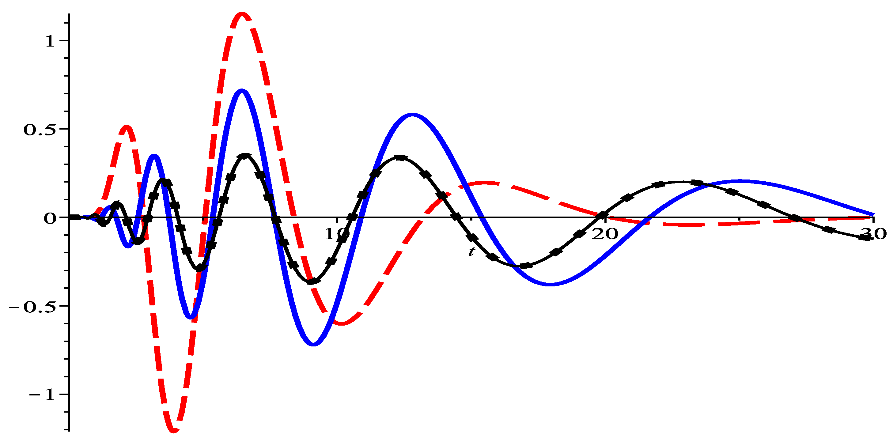
4. Convergence of MADEs to Classical Solutions

In this section, we present another example where we can study convergence of a MADE solution to its classical analogue. This requires an apriori uniform bound in a fixed neighborhood of $t=0$ for all $q>1$ sufficiently small. Obtaining a uniform-in-q bound for general $f_{\mu ,\lambda }(t)$ is rather deep, and complicated by the presence of the alternation ${(-1)}^m$ in Equation (42). Here we study a series without this alternating factor, which defines a function that behaves like a damped oscillation. The details are more challenging than what appears in the proof of Proposition 1, so a full analysis is provided.

Consider the following linear third-order MADE

$$f^{(3)}(t)=q^{3}f(qt)$$

(80)

for $q>1$, on the interval $t\in [0,\infty )$, satisfying the initial conditions

$$f(0)=0,f^{\prime }(0)=1,f^{″}(0)=-q.$$

(81)

For small $q>1$, as $q\to 1^{+}$, Equations (80) and (81) can be considered to be a perturbation of the classical analogue, which is the ODE

$$g^{(3)}(t)=g(t)$$

(82)

with initial conditions

$$g(0)=0,g^{\prime }(0)=1g^{″}(0)=-1$$

(83)

obtained by setting $q=1$ in (80) and (81). One can check directly that (82) and (83) is solved uniquely by

$$g(t)=2·exp(-t/2)·sin(\sqrt{3}t/2)/\sqrt{3}.$$

(84)

Now, using techniques mirroring those of Theorem 3.2 of [29], a particular solution to (80) is

$$\tilde{f}(t)=\sum _{k=-\infty }^{\infty }\frac{{\mathrm{e}}^{-q^{k}t/2}sin(\sqrt{3}{q}^{k}t/2)}{q^{k(k-1)/(2/3)}},$$

(85)

for $t\ge 0$. Note that the expression in Equation (85) does not have the alternation ${(-1)}^k$, unlike the expression in Equation (55) for $\eta (t)$, and this will allow a sharp bound on $\tilde{f}(t)$ for all $t\ge 0$, independent of $q>1$.

The first derivative of $\tilde{f}(t)$ is seen to be

$$\begin{array}{ccc}\hfill {\tilde{f}}^{\prime }(t)& =& \sum _{k=-\infty }^{\infty }\frac{q^k{\mathrm{e}}^{-q^{k}t/2}[(-1/2)sin(\sqrt{3}{q}^{k}t/2)+(\sqrt{3}/2)cos(\sqrt{3}{q}^{k}t/2)]}{q^{k(k-1)/(2/3)}}\hfill \\ \hfill & =& \sum _{k=-\infty }^{\infty }\frac{{\mathrm{e}}^{-q^{k}t/2}sin(\sqrt{3}{q}^{k}t/2+2\pi /3)}{q^{k(k-1-2/3)/(2/3)}}\hfill \end{array}$$

(86)

where the fact that:

$$\frac{-sin(x)+\sqrt{3}cos(x)}{2}=cos(2\pi /3)sin(x)+sin(2\pi /3)cos(x)=sin(x+2\pi /3),$$

was used explicitly to obtain the last equality in (86). Using this identity implicitly, we obtain:

$$\begin{array}{ccc}\hfill {\tilde{f}}^{(2)}(t)& =& \sum _{k=-\infty }^{\infty }\frac{q^k{\mathrm{e}}^{-q^{k}t/2}sin(\sqrt{3}{q}^{k}t/2+4\pi /3)}{q^{k(k-1-2/3)/(2/3)}}\hfill \\ \hfill & =& \sum _{k=-\infty }^{\infty }\frac{{\mathrm{e}}^{-q^{k}t/2}sin(\sqrt{3}{q}^{k}t/2+4\pi /3)}{q^{k(k-1-4/3)/(2/3)}}\hfill \end{array}$$

(87)

and finally we verify:

$$\begin{array}{}\mathrm{(88)}& \hfill {\tilde{f}}^{(3)}(t)& =& \sum _{k=-\infty }^{\infty }\frac{{\mathrm{e}}^{-q^{k}t/2}sin(\sqrt{3}{q}^{k}t/2+6\pi /3)}{q^{k(k-1-6/3)/(2/3)}}\hfill & & =& \sum _{k=-\infty }^{\infty }\frac{{\mathrm{e}}^{-q^{k-1}(qt)/2}sin(\sqrt{3}{q}^{k-1}qt/2)}{q^{[\{(k-1)+1\}][\{(k-1)-1\}-1]/(2/3)}}\hfill & & =& \sum _{m=-\infty }^{\infty }\frac{{\mathrm{e}}^{-q^m(qt)/2}sin(\sqrt{3}{q}^m(qt)/2)}{q^{[m+1][\{m-1\}-1]/(2/3)}}\hfill \mathrm{(89)}& \hfill & =& q^3\sum _{m=-\infty }^{\infty }\frac{{\mathrm{e}}^{-q^m(qt)/2}sin(\sqrt{3}{q}^m(qt)/2)}{q^{m(m-1)/(2/3)}}=q^3\tilde{f}(qt).\hfill \end{array}$$

A re-indexing $m=k-1$ was used to move from (88) to (89). Note that (89) gives that (80) holds. From (85)–(87), one sees that

$$\begin{array}{ccc}\hfill \tilde{f}(0)& =& \sum _{k=-\infty }^{\infty }\frac{sin(0)}{q^{k(k-1)/(2/3)}}=0,\hfill \end{array}$$

(90)

$$\begin{array}{ccc}\hfill {\tilde{f}}^{\prime }(0)& =& \sum _{k=-\infty }^{\infty }\frac{sin(2\pi /3)}{q^{k(k-5/3)/(2/3)}}=\frac{\sqrt{3}}{2}\sum _{k=-\infty }^{\infty }\frac{q^k}{{(q^3)}^{k(k-1)/2}}=\frac{\sqrt{3}}{2}\theta (q^3;q)\hfill \end{array}$$

(91)

$$\begin{array}{ccc}\hfill {\tilde{f}}^{(2)}(0)& =& \sum _{k=-\infty }^{\infty }\frac{sin(4\pi /3)}{q^{k(k-7/3)/(2/3)}}=\frac{-\sqrt{3}}{2}\sum _{k=-\infty }^{\infty }\frac{{(q^2)}^k}{{(q^3)}^{k(k-1)/2}}=\frac{-\sqrt{3}}{2}\theta (q^3;q^2),\hfill \end{array}$$

(92)

where the last equalities of (91) and (92) are obtained from (8).

Normalizing $\tilde{f}(t)$ by ${\tilde{f}}^{\prime }(0)=(\sqrt{3}/2)\theta (q^3;q)$ to obtain

$$f(t)=\tilde{f}(t)/{\tilde{f}}^{\prime }(0),$$

(93)

one sees that $f(t)$ now satisfies the MADE (80) along with the initial conditions (81). The last initial condition follows from the fact that

$$f^{(2)}(0)=\frac{{\tilde{f}}^{(2)}(0)}{{\tilde{f}}^{(1)}(0)}=\frac{-(\sqrt{3}/2)\theta (q^3;q^2)}{(\sqrt{3}/2)\theta (q^3;q)}=\frac{-\theta (q^3;q^2)}{\theta (q^3;q)}=-q,$$

(94)

where the last equality in (94) follows from the next lemma.

Lemma 1.

For $q>1$ the Jacobi theta function (8) satisfies

$$\frac{\theta (q^3;q^2)}{\theta (q^3;q)}=q=\frac{\theta (q^3;-q^2)}{\theta (q^3;-q)}.$$

(95)

Proof. 

For the first equality in (95) one can write

$$\theta (q^3;q^2)=\theta (q^3;q^3(1/q))=q^3(1/q)\theta (q^3;1/q)=q\left[q\theta (q^3;1/q)\right]=q\left[\theta (q^3;q)\right],$$

(96)

where the second equality is obtained from Equation (9) with $u=(1/q)$, and the last equality is the reciprocal identity in Equation (9) with $v=q$. Dividing (96) by $\theta (q^3;q)$ gives (95). For the second equality in (95), let $u=(-1/q)$ and $v=-q$ in Equation (9). Then as above $\theta (q^3;-q^2)=q\theta (q^3;-q)$. The lemma is shown. □

In addition to the last equality of (94) being proven by the first equality in (95) in Lemma 1, the second equality of (95) proves that the second derivative of ${\mathcal{W}}_{1,2/3}(t)/{\mathcal{W}}_{1,2/3}^{\prime }(0)$ at $t=0$ equals $-q$.

The following theta function bound will also be helpful.

Lemma 2.

For $q>1$ the Jacobi theta function (8) satisfies

$$\frac{\theta (q^3;1)}{\theta (q^3;q)}\le 1+\frac{1}{q^3}<2.$$

(97)

Proof. 

Observe that

$$\begin{array}{ccc}\hfill \theta (q^3;1)& =& {\mu }_{q^3}\prod _{n=0}^{\infty }\left[\left(1+\frac{1}{q^{3n}}\right)\left(1+\frac{1}{q^{3(n+1)}}\right)\right]\hfill \\ \hfill & =& {\mu }_{q^3}\left[\prod _{n=0}^{\infty }\left(1+\frac{1}{q^{3n}}\right)\right]\left(1+\frac{1}{q^3}\right)\left[\prod _{n=0}^{\infty }\left(1+\frac{1}{q^{6+3n}}\right)\right],\hfill \end{array}$$

(98)

while

$$\begin{array}{ccc}\hfill \theta (q^3;q)& =& {\mu }_{q^3}\prod _{n=0}^{\infty }\left[\left(1+\frac{q}{q^{3n}}\right)\left(1+\frac{1}{q{q}^{3(n+1)}}\right)\right]\hfill \\ \hfill & =& {\mu }_{q^3}\left[\prod _{n=0}^{\infty }\left(1+\frac{q}{q^{3n}}\right)\right]\left[\prod _{n=0}^{\infty }\left(1+\frac{1}{q^{4+3n}}\right)\right].\hfill \end{array}$$

(99)

Comparing each factor in the square brackets in (98) with the corresponding factor in the square brackets of (99) one sees that for all $n\ge 0$

$$\left(1+\frac{1}{q^{3n}}\right)\le \left(1+\frac{q}{q^{3n}}\right)\mathrm{and}\left(1+\frac{1}{q^{6+3n}}\right)\le \left(1+\frac{1}{q^{4+3n}}\right),$$

(100)

from which one concludes that

$$\frac{\theta (q^3;1)}{1+1/q^3}\le \theta (q^3;q),$$

(101)

giving the left inequality in (97). The right inequality in (97) holds via the assumption that $q>1$. □

Next we compute all derivatives of $g(t)=2exp(-t/2)sin(\sqrt{3}t/2)/\sqrt{3}$ at $t=0$ and of $f(t)=\tilde{f}(t)/{\tilde{f}}^{\prime }(0)$ at $t=0$, in preparation for the computation of the Taylor series expansion at $t=0$ for both $g(t)$ and $f(t)$. From (82) we immediately have that for $k\ge 0$ and $j=0,1,2$

$$g^{(3k+j)}(t)=g^{(j)}(t).$$

(102)

From (102) and (83) one concludes that for $k\ge 0$

$$g^{(3k)}(0)=g(0)=0,g^{(3k+1)}(0)=g^{\prime }(0)=1,g^{(3k+2)}(0)=g^{″}(0)=-1.$$

(103)

The analogous results for $f(t)=\tilde{f}(t)/{\tilde{f}}^{\prime }(0)$ are obtained in the following lemma.

Lemma 3.

For $t\ge 0$ and $q>1$, let $f(t)=\tilde{f}(t)/{\tilde{f}}^{\prime }(0)$ with $\tilde{f}(t)$ given by (85). Then for $k\ge 0$ and $j=0,1,2$ one has

$$f^{(3k+j)}(t)={\left(q^3\right)}^{k(k+1)/2}{q}^{jk}{f}^{(j)}(q^{k}t).$$

(104)

Furthermore, at $t=0$ one has

$$f^{(3k)}(0)=0,f^{(3k+1)}(0)={\left(q^3\right)}^{k(k+1)/2}{q}^k,f^{(3k+2)}(0)=-{\left(q^3\right)}^{k(k+1)/2}{q}^{2k}q.$$

(105)

Proof. 

We first establish (104) for the case that $j=0$ by induction on k. So for $j=0$ note that (104) holds as a tautology for $k=0$, and for $k=1$ it holds by (89). Assume that $f^{(3k)}(t)={\left(q^3\right)}^{k(k+1)/2}f(q^{k}t)$ for fixed k. Then

$$\begin{array}{}\mathrm{(106)}& \hfill f^{3(k+1)}(t)& =& f^{(3k+3)}(t)={\left[f^{(3k)}(t)\right]}^{(3)}={\left[{\left(q^3\right)}^{k(k+1)/2}f(q^{k}t)\right]}^{(3)}\hfill \mathrm{(107)}& \hfill & =& {\left(q^3\right)}^{k(k+1)/2}{q}^{3}f(q{q}^{k}t)q^{3k}={\left(q^3\right)}^{(k+1)(k+2)/2}f(q^{k+1}t),\hfill \end{array}$$

where: the inductive hypothesis gives the rightmost equality in (106), and that (89) along with the chain rule gives the first equality in (107). Thus, the $j=0$ case holds for all k. Now differentiate the expression $f^{(3k)}(t)={\left(q^3\right)}^{k(k+1)/2}f(q^{k}t)$ either $j=1$ or $j=2$ times to obtain (104) in all remaining cases. Evaluating (104) at $t=0$ and relying on (90)–(94) gives (105). □

Next, the $3N+2$-degree Taylor polynomials $P_{3N}[g](t),P_{3N}[f](t)$ of g and f, respectively, expanded about $t=0$ are given by

$$\begin{array}{ccc}\hfill P_{3N+2}[g](t)& =& \sum _{n=0}^{3N+2}\frac{g^{(n)}(0)}{n!}{t}^n=\sum _{k=0}^N\frac{g^{(3k)}(0)}{(3k)!}{t}^{3k}+\sum _{k=0}^N\frac{g^{(3k+1)}(0)}{(3k+1)!}{t}^{3k+1}\hfill \\ \hfill & \hfill & +\sum _{k=0}^N\frac{g^{(3k+2)}(0)}{(3k+2)!}{t}^{3k+2}\hfill \\ \hfill & =& \sum _{k=0}^N\frac{1}{(3k+1)!}{t}^{3k+1}+\sum _{k=0}^N\frac{-1}{(3k+2)!}{t}^{3k+2}\hfill \end{array}$$

(108)

$$\begin{array}{ccc}\hfill P_{3N+2}[f](t)& =& \sum _{n=0}^{3N+2}\frac{f^{(n)}(0)}{n!}{t}^n=\sum _{k=0}^N\frac{f^{(3k)}(0)}{(3k)!}{t}^{3k}+\sum _{k=0}^N\frac{f^{(3k+1)}(0)}{(3k+1)!}{t}^{3k+1}\hfill \\ \hfill & \hfill & +\sum _{k=0}^N\frac{f^{(3k+2)}(0)}{(3k+2)!}{t}^{3k+2}\hfill \\ \hfill & =& \sum _{k=0}^N\frac{q^{3k(k+1)/2}{q}^k}{(3k+1)!}{t}^{3k+1}+\sum _{k=0}^N\frac{-q^{3k(k+1)/2}{q}^{2k}q}{(3k+2)!}{t}^{3k+2}\hfill \end{array}$$

(109)

where (108) follows from (103), and (109) follows from (105). For $t\ge 0$, these have respective remainder terms

$$\begin{array}{ccc}\hfill R_{3N+2}[g](t)& =& \frac{g^{(3N+3)}(\xi )}{(3N+3)!}{t}^{3N+3}=\frac{g(\xi )}{(3N+3)!}{t}^{3N+3},\hfill \end{array}$$

(110)

$$\begin{array}{ccc}\hfill R_{3N+2}[f](t)& =& \frac{f^{(3N+3)}(\zeta )}{(3N+3)!}{t}^{3N+3}=\frac{q^{3(N+1)(N+2)/2}f(q^{N+1}\zeta )}{(3N+3)!}{t}^{3N+3}\hfill \end{array}$$

(111)

for some $\xi \in [0,t]$ and $\zeta \in [0,t]$. The goal of uniform convergence on compact subsets is now obtained in the following proposition.

Proposition 4.

Let S be any compact set contained in $[0,\infty )$. Then $f(t)$ converges uniformly to $g(t)$ on S as $q\to 1^{+}$, where $f(t)$ is given by both (93) and (85), while $g(t)$ is given by (84).

Proof. 

Without loss of generality, there is a $\rho >0$ such that $S\subseteq [0,\rho ]$, and it is sufficient to prove uniform convergence on $[0,\rho ]$. For $t\in [0,\rho ]$, from the triangle inequality one has

$$\begin{array}{}& \hfill \left|f(t)-g(t)\right|& \le & \left|f(t)-P_{3N+2}[f](t)\right|+\left|P_{3N+2}[f](t)-P_{3N+2}[g](t)\right|\hfill \mathrm{(112)}& & & +\left|P_{3N+2}[g](t)-g(t)\right|\hfill & & =& \left|R_{3N+2}[f](t)\right|+\left|P_{3N+2}[f](t)-P_{3N+2}[g](t)\right|\hfill \mathrm{(113)}& & & +\left|R_{3N+2}[g](t)\right|\hfill \end{array}$$

Now for $0\le t\le \rho$ and relying on (111), one starts with (114) to see

$$\begin{array}{}\mathrm{(114)}& \hfill \left|R_{3N+2}[f](t)\right|& =& \left|\frac{q^{3(N+1)(N+2)/2}f(q^{N+1}\zeta )}{(3N+3)!}{t}^{3N+3}\right|\hfill & & \le & \frac{q^{3(N+1)(N+2)/2}{\rho }^{3N+3}}{(3N+3)!}\left|f(q^{N+1}\zeta )\right|\hfill \mathrm{(115)}& & =& \frac{q^{3(N+1)(N+2)/2}{\rho }^{3N+3}}{(3N+3)!}\left|\frac{1}{\tilde{f}(0)}\tilde{f}(q^{N+1}\zeta )\right|\hfill \mathrm{(116)}& & =& \frac{q^{3(N+1)(N+2)/2}{\rho }^{3N+3}}{(3N+3)!}\times \hfill & & & \left|\frac{1}{(\sqrt{3}/2)\theta (q^3;q)}\sum _{k=-\infty }^{\infty }\frac{{\mathrm{e}}^{-q^k{q}^{N+1}\zeta /2}sin(\sqrt{3}{q}^k{q}^{N+1}\zeta /2)}{q^{k(k-1)/(2/3)}}\right|\hfill \mathrm{(117)}& & \le & \frac{q^{3(N+1)(N+2)/2}{\rho }^{3N+3}}{(3N+3)!}\frac{2}{\sqrt{3}\theta (q^3;q)}\sum _{k=-\infty }^{\infty }\frac{1}{{\left(q^3\right)}^{k(k-1)/(2)}}\hfill \mathrm{(118)}& & =& \frac{q^{3(N+1)(N+2)/2}{\rho }^{3N+3}}{(3N+3)!}\frac{2}{\sqrt{3}\theta (q^3;q)}\theta (q^3;1)\hfill \mathrm{(119)}& & <& \frac{q^{3(N+1)(N+2)/2}{\rho }^{3N+3}}{(3N+3)!}\frac{4}{\sqrt{3}},\hfill \end{array}$$

where: moving to (115) is obtained via (93); (116) follows from (85) and (91); the equality in (118) is obtained by (8); and the inequality in (119) is given by (97) in Lemma 2. Similarly, from (110) and (84), one has

$$\begin{array}{ccc}\hfill \left|R_{3N+2}[g](t)\right|& =& \left|\frac{g(\xi )}{(3N+3)!}{t}^{3N+3}\right|\hfill \\ \hfill & \le & \frac{{\rho }^{3N+3}}{(3N+3)!}\left|2exp(-\xi /2)sin(\sqrt{3}\xi /2)/\sqrt{3}\right|\le \frac{2{\rho }^{3N+3}}{\sqrt{3}(3N+3)!}.\hfill \end{array}$$

(120)

Also, from (108) and (109) if we let: $\Delta P[f,g](t)\equiv P_{3N+2}[f](t)-P_{3N+2}[g](t)$, then

$$\begin{array}{ccc}\hfill \left|\Delta P[f,g](t)\right|& =& \left|\sum _{k=0}^N\frac{q^{3k(k+1)/2}{q}^k-1}{(3k+1)!}{t}^{3k+1}+\sum _{k=0}^N\frac{-q^{3k(k+1)/2}{q}^{2k}q+1}{(3k+2)!}{t}^{3k+2}\right|\hfill \\ \hfill & \le & \sum _{k=0}^N\frac{q^{3k(k+1)/2}{q}^k-1}{(3k+1)!}{\rho }^{3k+1}+\sum _{k=0}^N\frac{q^{3k(k+1)/2}{q}^{2k}q-1}{(3k+2)!}{\rho }^{3k+2}\hfill \\ \hfill & \le & \left[q^{3N(N+1)/2}{q}^{2N}q-1\right]\left[\sum _{k=0}^N\frac{{\rho }^{3k+1}}{(3k+1)!}+\sum _{k=0}^N\frac{{\rho }^{3k+2}}{(3k+2)!}\right]\hfill \\ \hfill & \le & \left[q^{3N(N+1)/2}{q}^{2N}q-1\right]{\mathrm{e}}^{\rho }.\hfill \end{array}$$

(121)

Applying (118), (121), and (120) to (113) one has that for $N\ge 0$

$$\begin{array}{ccc}\hfill \left|f(t)-g(t)\right|& \le & \frac{q^{3(N+1)(N+2)/2}{\rho }^{3N+3}}{(3N+3)!}\frac{4}{\sqrt{3}}\hfill \\ \hfill & & +\left[q^{3N(N+1)/2}{q}^{2N}q-1\right]{\mathrm{e}}^{\rho }+\frac{2{\rho }^{3N+3}}{\sqrt{3}(3N+3)!}.\hfill \end{array}$$

(122)

Now, given $ϵ>0$, choose $N_0$ sufficiently large such that one has $4{\rho }^{3N_0+3}/\left[\sqrt{3}(3N_0+3)!\right]<ϵ/3$. Then

$$1<(ϵ/3)\left[\sqrt{3}(3N_0+3)!\right]/\left[4{\rho }^{3N_0+3}\right]\mathrm{and}1<1+ϵ/\left[3{\mathrm{e}}^{\rho }\right].$$

Pick $q_0>1$ so that

$$q_0^{3(N_0+1)(N_0+2)/2}<(ϵ/3)\left[\sqrt{3}(3N_0+3)!\right]/\left[4{\rho }^{3N_0+3}\right]$$

(123)

and

$$q_0^{3N_0(N_0+1)/2}{q}_0^{2N_0}{q}_0<1+ϵ/\left[3{\mathrm{e}}^{\rho }\right].$$

Then for $1<q<q_0$ one has

$$q^{3(N_0+1)(N_0+2)/2}<(ϵ/3)\left[\sqrt{3}(3N_0+3)!\right]/\left[4{\rho }^{3N_0+3}\right]$$

(124)

and

$$q^{3N_0(N_0+1)/2}{q}^{2N_0}q<1+ϵ/\left[3{\mathrm{e}}^{\rho }\right],$$

whence for $1<q<q_0$

$$\frac{2{\rho }^{3N_0+3}}{\sqrt{3}(3N_0+3)!}<q^{3(N_0+1)(N_0+2)/2}\frac{4{\rho }^{3N_0+3}}{\sqrt{3}(3N_0+3)!}<(ϵ/3)$$

(125)

and

$$\left[q^{3N_0(N_0+1)/2}{q}^{2N_0}q-1\right]{\mathrm{e}}^{\rho }<ϵ/3.$$

Applying (125) to (122) with N taken to be $N_0$ one has that for $1<q<q_0$

$$\left|f(t)-g(t)\right|\le ϵ/3+ϵ/3+ϵ/3=ϵ.$$

(126)

So $f(t)$ approaches $g(t)$ uniformly on $[0,\rho ]$ as $q\to 1^{+}$, and the proposition is proven. □

5. Convolutions, Correlations and Bounds

Here we briefly demonstrate that solutions of MADEs beget new solutions of different MADEs.

5.1. Distinction between Convolutions and Correlations

Let $f,g\in {\mathcal{L}}^1(\mathbb{R})$ and recall the standard definitions:

$$\begin{array}{ccc}\hfill \mathrm{Convolution}\mathrm{between}f\mathrm{and}g& \equiv & \left[f\ast g\right](t)={\int }_{-\infty }^{\infty }f(s)·g(t-s)ds\hfill \end{array}$$

(127)

$$\begin{array}{ccc}\hfill \mathrm{Correlation}\mathrm{between}f\mathrm{and}g& \equiv & \left[f\star g\right](t)={\int }_{-\infty }^{\infty }f(s)·g(t+s)ds\hfill \end{array}$$

(128)

Proposition 5.

Consider $f,g\in \mathcal{S}(\mathbb{R})$, which solve the following MADEs

$$f^{(a)}=c_f·f(qt),g^{(b)}=c_g·g(qt),$$

(129)

respectively, for $q>1$, $a,b\in \mathbb{N}$, and $c_f\ne 0$, $c_g\ne 0$. Then the correlation and convolution solve the following higher-order MADEs

$${\left[f\ast g\right]}^{(a+b)}(t)=\frac{c_f·c_g}{q}\left[f\ast g\right](qt),{\left[f\star g\right]}^{(a+b)}(t)={(-1)}^a\frac{c_f·c_g}{q}\left[f\star g\right](qt),$$

and $\left[f\ast g\right],\left[f\star g\right]\in \mathcal{S}(\mathbb{R})$.

Proof. 

The fact that convolution and correlation preserve the Schwartz property follows from Theorem 3.3 of [31]. The MADE equations easily follow from repeated applications of integration by parts, use of Equation (129), and a change of variables. □

5.2. Auto-Correlation

It was shown in Theorem 7 of [25] that the auto-correlation of ${\mathcal{W}}_{-1,2}(t)=F_{-1,2}(t)$, as defined in (45) for $\mu =-1$ and $\lambda =2$, gives ${\mathcal{W}}_{0,1}(t)=f_{0,1}(|t|)$, as defined in (42) for $\mu =0$ and $\lambda =1$, in the sense that

$$\begin{array}{ccc}\hfill [{\mathcal{W}}_{-1,2}\star {\mathcal{W}}_{-1,2}](t)& \equiv & {\int }_{-\infty }^{\infty }{\mathcal{W}}_{-1,2}(u)·{\mathcal{W}}_{-1,2}(u+t)du\hfill \\ & =& \frac{-{\mu }_q^4}{2{\mu }_{q^2}^2}·{\mathcal{W}}_{-2,1}(-t)=\frac{-{\mu }_q^4}{2{\mu }_{q^2}^2}·{\mathcal{W}}_{-2,1}(t)=\frac{+{\mu }_q^4}{2{\mu }_{q^2}^2}·{\mathcal{W}}_{0,1}\left(\frac{t}{q}\right),\hfill \end{array}$$

where ${\mathcal{W}}_{-2,1}(t)=f_{-2,1}(|t|)$, as defined in (42) for $\mu =-2$ and $\lambda =1$. Using this result, along with the Cauchy-Schwartz inequality it was shown in Proposition 4 of [25] that

$$0<\parallel {\mathcal{W}}_{0,1}{\parallel }_{\infty }={\mathcal{W}}_{0,1}(0)=\theta (q^2;-1/q)<1,\forall q>1.$$

This important bound allows one to obtain uniform convergence of the normalized function ${\mathcal{W}}_{0,1}(t)/{\mathcal{W}}_{0,1}(0)\to cos(t)$, as $q\to 1^{+}$.

5.3. Cross-Correlation

Let us consider an example that involves different MADE solutions, to obtain a new MADE. Knowing the Fourier transform of these functions allows us to easily derive properties of the resulting function. Compute, using Plancherel’s Lemma,

$$\begin{array}{ccc}\hfill [{\mathcal{W}}_{-1,2}\star {\mathcal{W}}_{0,1}](t)& \equiv & {\int }_{-\infty }^{\infty }{\mathcal{W}}_{-1,2}(u)·{\mathcal{W}}_{0,1}(u+t)du\hfill \\ & =& {\int }_{-\infty }^{\infty }{e}^{-i\omega t}\mathcal{F}[{\mathcal{W}}_{-1,2}](\omega )·\mathcal{F}[{\mathcal{W}}_{0,1}](\omega )d\omega .\hfill \end{array}$$

(130)

Now, to simplify the integrand in (130), we use the Fourier transforms from [25,32] respectively, to write:

$$\begin{array}{ccc}\hfill \mathcal{F}[{\mathcal{W}}_{-1,2}](\omega )·\mathcal{F}[{\mathcal{W}}_{0,1}](\omega )& =& \frac{i{\mu }_q^3}{\sqrt{2\pi }\omega \theta (q;i\omega )}\times \frac{2{({\mu }_{q^2})}^3}{\sqrt{2\pi }\theta (q^2;{\omega }^2)}\hfill \\ \hfill & =& \frac{i{({\mu }_q·{\mu }_{q^2})}^3}{\pi }\times \frac{1}{\omega \theta (q;i\omega )\theta (q^2;{\omega }^2)}\hfill \\ \hfill & =& \frac{{({\mu }_q^2·{\mu }_{q^2})}^2}{\pi }\times \frac{1}{(-i\omega )\theta (q;-i\omega ){\theta }^2(q;i\omega )}.\hfill \end{array}$$

(131)

The equality in (131) follows from the fact that $\theta (q^2;{\omega }^2)=\theta (q;i\omega )\theta (q;-i\omega )$ and uses the definition of the Jacobi theta function in Equation (8). The consequence is that there are simple poles when $\omega =-i{q}^k$ for $k\in \mathbb{Z}$, but double poles at $\omega =i{q}^k$. Computing the integral in (130) using residue theory, requires a careful consideration of the position of these poles off the real axis.

For $t\ge 0$ the contour for $\omega$ must traverse the lower-half plane, encompassing the simple poles $\omega =-i{q}^k$. Consequently, residue theory and Equation (9) gives

$$[{\mathcal{W}}_{-1,2}\star {\mathcal{W}}_{0,1}](t)=C_q\sum _{k=-\infty }^{\infty }{(-1)}^k\frac{e^{-q^{k}t}}{q^{3k(k+1)/2}}=C_q·f_{-1,2/3}(t),$$

which solves the eigen-MADE

$$f_{-1,2/3}^{(3)}(t)=f_{-1,2/3}(qt).$$

6. Expanded Table of Fourier Transforms

In this final section we establish a short table of Fourier transforms for solutions of MADEs and their relations to Jacobi theta functions. Included are well-established results, along with new functions. The positive constants $K_1$ and $K_2$ are generic, but estimates are not presented here.

The introduction of new functions are as follows: For $K(t)$ see [32] for decay constants $K_1$ and $K_2$ in

Table 1. Table of Fourier transforms with solutions of ODEs and MADEs.

Global Function	Property	Differential Equation	$\mathit{f}(0)$	$\mathit{f}(\pm \infty )$ Decay Rate	Fourier Transf. (Modulo Coef.)
$f(t)=e^{-t^2/2}$	Entire Schwartz	$-f^{″}(t)+t^{2}f(t)=f(t)$	1	Gaussian	$e^{-x^2/2}$
$f(t)=e^{-|t|}$	$C^0\cap {\mathcal{L}}^p$ $1\le p\le \infty$	$f^{\prime }(t)+f(t)=-2\delta (t)$	1	exponential	${(1+x^2)}^{-1}$
$e^{i(x-x_0)t}=$ $exp[i(x-x_0)t]$	$C^0\cap {\mathcal{L}}^{\infty }$	${\partial }_{t}exp[i(x-x_0)t]=$ $i(x-x_0)exp[i(x-x_0)t]$	1	undefined	${\delta }_0(x-x_0)={\delta }_{x_0}(x)$
$j_0(t)=\frac{sin(t)}{t}$	$C^{\infty }\cap {\mathcal{L}}^p$ $1<p\le \infty$	$j_0^{″}(t)+\frac{2}{t}{j}_0^{\prime }(t)=-j_0(t)$	1	$1/|t|$	${\chi }_{[-1,1]}(x)$
$Ai(t)=$ ${\int }_0^{\infty }cos(\frac{u^3}{3}+ut)du$	$C^{\infty }\cap {\mathcal{L}}^p$ $4<p\le \infty$	$A{i}^{″}(t)=t·Ai(t)$	Ai(0) smooth	$1/{|t|}^{1/4}$	$e^{ik{x}^3/3}$
$cos(t)$ $sin(t)$	$C^0\cap {\mathcal{L}}^{\infty }$	${cos}^{″}(t)+cos(t)=0$ ${sin}^{″}(t)+sin(t)=0$	1	undefined	${\delta }_1(x)\pm {\delta }_{-1}(x)$
$K(t)\equiv F_{-1,2}(t)$	Schwartz wavelet	$K^{\prime }(t)=K(qt)$	0 flat	${|t|}^{-K_{1}ln|t|+K_2}$	$\frac{1}{ix\theta (q;ix)}$
${\tilde{C}}_q(t)=$ $f_{0,1}(\frac{|t|}{\sqrt{q}})/f_{0,1}(0)$	Schwartz wavelet	${\tilde{C}}_q^{\prime \prime }(t)+{\tilde{C}}_q(qt)=0$	1 smooth	${|t|}^{-K_{3}ln|t|+K_4}$	$\frac{1}{\theta (q^2;q{x}^2)}$
${\tilde{S}}_q(t)={\int }_0^t{\tilde{C}}_q(u)du$	Schwartz wavelet	${\tilde{S}}_q^{\prime \prime }(t)+q^{-1}{\tilde{S}}_q(qt)=0$	0 smooth	${|t|}^{-K_{3}ln|t|+K_4}$	$\frac{-i{q}^{3}x}{\theta (q^2;q^3{x}^2)}$
$Ci{S}_q(t)=$ ${\tilde{C}}_q(t)+i{\tilde{S}}_q(t)$	Schwartz wavelet	${\partial }_t^{2}Ci{S}_q(t)=-Ci{S}_q(qt)$	1 smooth	${|t|}^{-K_{3}ln|t|+K_4}$	$\frac{1}{\theta (q^2;q{x}^2)}$ + $\frac{q^{3}x}{\theta (q^2;q^3{x}^2)}$
$\mathcal{J}(t)=\frac{{\tilde{S}}_q(t)}{t}$	Schwartz	${\mathcal{J}}^{″}(t)+\frac{2}{t}{\mathcal{J}}^{\prime }(t)=-\mathcal{J}\left(qt\right)$	$1/q$	${|t|}^{-K_{5}ln|t|+K_6}$	${\int }_{-\infty }^x\frac{\omega d\omega }{\theta (q^2;q^3{\omega }^2)}$
$F(t)=F_{2M+1,2N}(t)$	Schwartz wavelet	$a=N+1$ $b=(N+2M+1)/2$ $F^{\prime }(t)={(-1)}^a{q}^{b}F(q^{N}t)$	0 flat	${|t|}^{-K_{7}ln|t|+K_8}$	${(-z_j)}^N=-ix$ $\frac{-i}{xN}{\sum }_{j=1}^N\frac{z_j^{M+1}}{\theta (q^{1/N};z_j)}$
$M_1(t)=$ $[K\ast {\tilde{C}}_q](t)$	Schwartz wavelet	$M_1^{‴}(t)=-q^{-1}{M}_1(qt)$	0 smooth	${|t|}^{-K_{9}ln|t|+K_{10}}$	$\frac{1}{ix\theta (q;ix)\theta (q^2;q{x}^2)}$
$M_2(t)=$ ${\mathcal{W}}_{1,2/3}(t)$	Schwartz wavelet	$M_2^{‴}(t)=q^3{M}_2(qt)$	0 smooth	${|t|}^{-K_{9}ln|t|+K_{10}}$	$\frac{x^2}{\theta (q^3;-i{x}^3)}$
$Aiq(t)=$ ${\int }_0^{\infty }{\tilde{C}}_q(\frac{u^3}{3}+ut)du$	Schwartz	$Ai{q}^{″}(t)=$ $q^{-1/3}t·Aiq(q^{2/3}t)$	$Aiq(0)$ smooth	${|t|}^{-K_{3}ln|t|+K_4}$	${\int }_0^{\infty }$$\frac{e^{i{x}^3/(3k^2)}}{\theta (q^2;q{k}^2)}$ dk

; The functions ${}_{q}Cos(t)$ and ${}_{q}Sin(t)$ are closely related to ${\tilde{C}}_q(t)$ and ${\tilde{S}}_q(t)$, respectively, introducted in [25], where constants $K_3$ and $K_4$ are obtained; The q-Bessel functions, related to $\mathcal{J}(t)$, were introduced in [33], along with decay constants $K_5$ and $K_6$; Flat wavelets $F(t)$ have Fourier transforms that are averages of theta functions, first derived in [29], along with constants $K_7$ and $K_8$. The functions $K\ast {\tilde{C}}_q(t)$ and ${\mathcal{W}}_{\mu ,\lambda }(t)$, have Fourier transforms that involve theta functions, which can be used to obtain decay parameters $K_9$ and $K_{10}$.

Note that similar tables for Laplace transforms are quite extensive, since applications only require control of function growth on ${\mathbb{R}}^{+}$. Here we are concerned with globally defined functions on $\mathbb{R}$ for which a Fourier transform can be defined.

References

1. Burden, R.L.; Fairs, D.J.; Burden, A.M. Numerical Analysis; 10E. Cengage Learning: Boston, MA, USA, 2016. [Google Scholar]
2. Fox, L.; Mayers, D.F.; Ockendon, J.R.; Tayler, A.B. On a Functional Differential Equation. IMA J. Appl. Math. 1971, 8, 271–307. [Google Scholar] [CrossRef]
3. Kato, T.; McLeod, J.B. The Functional-Differential Equation y′(x) = ay(λx) + by(x). Bull. Am. Math. Soc. 1971, 77, 891–937. [Google Scholar]
4. Reed, M.; Simon, B. Functional Analysis I; Academic Press: New York, NY, USA, 1975. [Google Scholar]
5. Dung, N.T. Asymptotic behavior of linear advanced differential equations. Acta Math. Sci. 2015, 35, 610–618. [Google Scholar] [CrossRef]
6. Di Vizio, L. An ultrametric version of the Maillet-Malgrange theorem for nonlinear q-difference equations. Proc. Am. Math. Soc. 2008, 136, 2803–2814. [Google Scholar] [CrossRef] [Green Version]
7. Di Vizio, L.; Hardouin, C. Descent for differential Galois theory of difference equations: Confluence and q-dependence. Pac. J. Math. 2012, 256, 79–104. [Google Scholar] [CrossRef] [Green Version]
8. Di Vizio, L.; Zhang, C. On q-summation and confluence. Ann. Inst. Fourier (Grenoble) 2009, 59, 347–392. [Google Scholar] [CrossRef]
9. Dreyfus, T. Building meromorphic solutions of q-difference equations using a Borel-Laplace summation. Int. Math. Res. Not. IMRN 2015, 15, 6562–6587. [Google Scholar] [CrossRef] [Green Version]
10. Dreyfus, T.; Lastra, A.; Malek, S. On the multiple-scale analysis for some linear partial q-difference and differential equations with holomorphic coefficients. Adv. Differ. Equ. 2019, 2019, 326. [Google Scholar] [CrossRef]
11. Lastra, A.; Malek, S. On q-Gevrey asymptotics for singularly perturbed q-difference-differential problems with an irreguular singularity. Abstr. Appl. Anal. 2012, 2012, 860716. [Google Scholar] [CrossRef]
12. Lastra, A.; Malek, S. On parametric Gevrey asymptotics for singularly perturbed partial differential equations with delays. Abstr. Appl. Anal. 2013, 2013, 723040. [Google Scholar] [CrossRef] [Green Version]
13. Lastra, A.; Malek, S. Parametric Gevrey asymptotics for some Cauchy problems in quasiperiodic function spaces. Abstr. Appl. Anal. 2014, 2014, 153169. [Google Scholar] [CrossRef] [Green Version]
14. Lastra, A.; Malek, S. On parametric multilevel q-Gevrey asymptotics for some linear q-difference-differential equations. Adv. Differ. Equ. 2015, 2015, 344. [Google Scholar] [CrossRef] [Green Version]
15. Lastra, A.; Malek, S. On multiscale Gevrey and q-Gevrey asymptotics for some linear q-difference differential initial value Cauchy problems. J. Differ. Equ. Appl. 2017, 23, 1397–1457. [Google Scholar] [CrossRef]
16. Lastra, A.; Malek, S. On a q-Analog of Singularly Perturbed Problem of Irregular Type with Two Complex Time Variables. Mathematics 2019, 2019, 924. [Google Scholar] [CrossRef]
17. Lastra, A.; Malek, S.; Sanz, J. On q-asymptotics for linear q-difference-differential equations with Fuchsian and irreguular singularities. J. Differ. Equ. 2012, 252, 5185–5216. [Google Scholar] [CrossRef]
18. Lastra, A.; Malek, S.; Sanz, J. On q-asymptotics for q-difference-differential equations with Fuchsian and irregular singularities, Formal and analytic solutions of differential and difference equations. Pol. Acad. Sci. Inst. Math. 2012, 97, 73–90. [Google Scholar]
19. Lastra, A.; Malek, S.; Sanz, J. On Gevrey solutions of threefold singular nonlinear partial differential equations. J. Differ. Equ. 2013, 255, 3205–3232. [Google Scholar] [CrossRef]
20. Malek, S. On complex singularity analysis for linear partial q-difference-differential equations using nonlinear differential equations. J. Dyn. Control Syst. 2013, 19, 69–93. [Google Scholar] [CrossRef]
21. Stéphane, M. On parametric Gevrey asymptotics for a q-analog of some linear initial value problem. Funkcial. Ekvac. 2017, 60, 21–63. [Google Scholar]
22. Malek, S. On a Partial q-Analog of a Singularly Perturbed Problem with Fuchsian and Irregular Time Singularity. Abstr. Appl. Anal. 2020, 2020, 7985298. [Google Scholar] [CrossRef] [Green Version]
23. Tahara, H. q-analogues of Laplace and Borel transforms by means of q-exponentials. Ann. Inst. Fourier Grenoble 2017, 67, 1865–1903. [Google Scholar] [CrossRef] [Green Version]
24. Zhang, C. Analytic continuation of solutions of the pantograph equation by means of θ-modular forms. arXiv 2012, arXiv:1202.0423. [Google Scholar]
25. Pravica, D.W.; Randriampiry, N.; Spurr, M.J. Reproducing kernel bounds for an advanced wavelet frame via the theta function. Appl. Comput. Harmon. Anal. 2012, 33, 79–108. [Google Scholar] [CrossRef] [Green Version]
26. Bender, C.M.; Orszag, S.A. Asymptotic Analysis; Advanced Mathematical Methods for Scientists and Engineers; Springer: New York, NY, USA, 1999. [Google Scholar]
27. Craig, W.; Goodman, J. Linear Dispersive Equations of Airy Type. J. Differ. Equ. 1990, 87, 38–61. [Google Scholar] [CrossRef] [Green Version]
28. Reed, M.; Simon, B. Fourier Analysis, Self-Adjointness II; Academic Press: New York, NY, USA, 1975. [Google Scholar]
29. Pravica, D.W.; Randriampiry, N.; Spurr, M.J. Solutions of a class of multiplicatively advanced differential equations. C.R. Acad. Sci. Paris Ser. I 2018, 356, 776–817. [Google Scholar] [CrossRef]
30. Pravica, D.; Spurr, M. Analytic Continuation into the Future. Discret. Contin. Dyn. Syst. 2003, 2003, 709–716. [Google Scholar]
31. Stein, E.; Weiss, G. Introduction to Fouier Analysis on Euclidian Spaces; Princeton University Press: Princeton, NJ, USA, 1971. [Google Scholar]
32. Pravica, D.; Randriampiry, N.; Spurr, M. Applications of an advanced differential equation in the study of wavelets. Appl. Comput. Harmon. Anal. 2009, 27, 2–11. [Google Scholar] [CrossRef] [Green Version]
33. Pravica, D.; Randriampiry, N.; Spurr, M. On q-advanced spherical Bessel functions of the first kind and perturbations of the Haar wavelet. Appl. Comput. Harmon. Anal. 2018, 44, 350–413. [Google Scholar] [CrossRef]
Figure 1. Three Flat Functions: Normalized plots of first-order MADE solutions that are flat at t = 0 , (1) f 1 , 2 ( t ) (dashed red), (2) f 1 , 4 ( t ) (solid blue), (3) f 1 , 6 ( t ) (dotted black line) all for q = 1.3 .
Axioms 09 00083 g001
Figure 2. (Left) Asymptotic extension ϕ ˜ ( t ) from Equation (73) for ϕ ( t ) (solid red) together with a similarly constructed asymptotic extension for χ ( , 0 ] ( t ) W 1 , 5 / 3 ( t ) / f 1 , 2 / 3 ( 0 ) (dashed blue) both for q = 1.2 . (Right) Plots of e t K ˜ ( t ) where the functions K ˜ ( t ) are defined in Equation (76) for q = 1.2 . Failure of the asymptotic extension is found to be around t = 1 , as compared to the computed value of t = 1.8 . The upper-sum limits, from left to right, are N = 6 , 10 ( d o t t e d ) , 20 , 30 .
Axioms 09 00083 g002