Solving a Quadratic Riccati Differential Equation, Multi-Pantograph Delay Differential Equations, and Optimal Control Systems with Pantograph Delays

Abstract

An effective algorithm for solving quadratic Riccati differential equation (QRDE), multipantograph delay differential equations (MPDDEs), and optimal control systems (OCSs) with pantograph delays is presented in this paper. This technique is based on Genocchi polynomials (GPs). The properties of Genocchi polynomials are stated, and operational matrices of derivative are constructed. A collocation method based on this operational matrix is used. The findings show that the technique is accurate and simple to use.

1. Introduction

Riccati differential equations (RDEs) play significant role in many fields of applied science [1]. For example, a one-dimensional static Schrödinger equation [2,3,4]. The applications of this equation found not only in random processes, optimal control, and diffusion problems [1] but also in stochastic realization theory, optimal control, network synthesis and financial mathematics. Now, RDEs attracted much attention. Recently, various iterative methods are employed for the numerical and analytical solution of functional equations such as Adomian’s decomposition method (ADM) (see [5,6]), homotopy perturbation method (HPM) [7], variational iteration method (VIM) [8], and differential transform method (DTM) [9].

The GPs are non-orthogonal polynomials, which were first applied to solve fractional calculus problem (FCP) involving differential equation [10], this GPs were successfully applied to solve different kinds of problems in numerical analysis, system of Volterra integro-differential equation [11] and fractional Klein-Gordon equation [12], differential topology (differential structures on spheres), theory of modular forms (Eisenstein series).

In this paper, a new operational matrix of fractional order derivative based on Genocchi polynomials is introduced to provide approximate solutions of QRDE. Although the method is very easy to utilize and straightforward, the obtained results are satisfactory (see the numerical results).

The outline of this sequel is as follows: In Section 2, Some basic preliminaries are stated. Explanation of the problem is explained in Section 3. Some numerical results are provided in Section 4. A remark is provided about MPDDEs and OCSs. Numerical applications for solving MPDDEs are stated in Section 5. Finally, Section 6 will give a conclusion briefly.

2. Some Basic Preliminaries

Genocchi numbers ($G_n$) and Genocchi polynomials ($G_n\left(x\right)$) have been extensively studied in various papers, (see [13]). The classical Genocchi polynomials $G_n\left(x\right)$ are usually defined by the following form

$$\begin{array}{c}\hfill \frac{2t{e}^{xt}}{e^t+1}=\sum _{i=0}^{\infty }{G}_n\left(x\right)\frac{t^n}{n!},\left(\right|t|<\pi ),\end{array}$$

(1)

where

$$\begin{array}{c}{G}_n\left(x\right)=\sum _{k=0}^n\left(\genfrac{}{}{0pt}{}{n}{k}\right)G_k{x}^{n-k},\hfill \\ G_1=1,G_2=0,G_3=0,G_4=1,G_5=0,G_6=-3,G_7=0,\hfill \\ G_8=17,G_9=0,G_{10}=-155,G_{11}=0,G_{12}=2073,\hfill \\ G_{2n+1}=0,n\in N,\hfill \\ G_1\left(x\right)=1,\hfill \\ G_2\left(x\right)=2x-1,\hfill \\ G_3\left(x\right)=3x^2-3x,\hfill \\ G_4\left(x\right)=4x^3-6x^2+1,\hfill \\ G_5\left(x\right)=5x^4-10x^3+5x,\hfill \\ G_6\left(x\right)=6x^5-15x^4+15x^2-3,\hfill \\ G_n(x+1)+G_n\left(x\right)=2n{x}^{n-1},n\ge 0,\hfill \\ \frac{d{G}_n\left(x\right)}{dx}=n{G}_{n-1}\left(x\right),n\ge 1,\hfill \\ {\int }_a^b{G}_n\left(x\right)dx=\frac{G_{n+1}\left(b\right)-G_{n+1}\left(a\right)}{n+1},\hfill \\ {\int }_0^1{G}_n\left(x\right)G_m\left(x\right)dx=\frac{2{(-1)}^{n}n!m!}{(n+m)!}{G}_{n+m},m,n\ge 1,\hfill \end{array}$$

(2)

from (2), we have

$$\begin{array}{c}{G}_n\left(x\right)={\int }_0^{x}n{G}_{n-1}\left(t\right)dt+G_n,n\ge 1,\hfill \end{array}$$

also, we have

$$\begin{array}{ccc}\hfill e^{tx}& =& \frac{1}{2t}(\frac{2t}{e^t+1}{e}^{(1+x)t}+\frac{2t}{e^t+1}{e}^{xt})\hfill \\ & =& \frac{1}{2t}\sum _{n=0}^{\infty }(G_n(x+1)+G_n\left(x\right))\frac{t^n}{n!}.\hfill \end{array}$$

3. Explanation of the Problem

Firstly, Riccati differential equation (RDE) is considered

$$\begin{array}{c}{y}^{\prime }\left(x\right)=p\left(x\right)-q\left(x\right)y\left(x\right)+r\left(x\right)y^2\left(x\right),x_0\le x\le x_f,\hfill \\ y\left(x_0\right)=\alpha ,\hfill \end{array}$$

(3)

where $p\left(x\right)$, $q\left(x\right)$ and $r\left(x\right)$ are continuous, $x_0$, $x_f$ and $\alpha$ are arbitrary constants, and $y\left(x\right)$ is unknown function.

Now, the collocation method based on Genocchi operational matrix of derivatives to solve numerically RDEs is presented.

Our strategy is utilizing Genocchi polynomials (GPs) to approximate the solution $y\left(x\right)$ by $y_N\left(x\right)$ is as given below.

$$\begin{array}{c}y\left(x\right)\approx y_N\left(x\right)=\sum _{n=1}^N{c}_n{G}_n\left(x\right)=G\left(x\right)C,\hfill \end{array}$$

where

$$\begin{array}{c}{C}^T=[c_1,c_2,\dots ,c_n],\hfill \end{array}$$

$$\begin{array}{c}G\left(x\right)=[G_1\left(x\right),G_2\left(x\right),\dots ,G_N\left(x\right)],\hfill \\ M=\left[\begin{array}{ccccccc}0& 0& 0& \dots & 0& 0& 0,\\ 2& 0& 0& \dots & 0& 0& 0\\ ⋮& ⋮& ⋮& ⋮& ⋮& ⋮& ⋮\\ 0& 0& 0& \dots & N-1& 0& 0\\ 0& 0& 0& \dots & 0& N& 0\end{array}\right]\hfill \end{array}$$

(4)

$$\begin{array}{c}{G}^{\prime }{\left(x\right)}^T=M{G}^T\left(x\right),\Rightarrow G^{\prime }\left(x\right)=G\left(x\right)M^T,\hfill \\ ⋮⋮\hfill \\ G^{\left(k\right)}\left(x\right)=G\left(x\right){\left(M^T\right)}^k,\hfill \end{array}$$

(5)

then, the k-th derivative of $y_N\left(x\right)$ can be stated as

$$\begin{array}{c}{y}_N^{\left(k\right)}\left(x\right)=G^{\left(k\right)}\left(x\right)C=G\left(x\right){\left(M^T\right)}^{k}C,\hfill \end{array}$$

(6)

by Equations (3) and (6), we have

$$\begin{array}{c}G\left(x\right)M^{T}C=p\left(x\right)-q\left(x\right)G\left(x\right)C+r\left(x\right){\left(G\left(x\right)C\right)}^2,\hfill \end{array}$$

(7)

to obtain $y_N\left(x\right)$, one may use the collocation points $x_j=\frac{j-1}{N}$, $j=1,2,\dots ,N-1$.

These equations can be solved by Maple 15 software.

Lemma 1.

If $y\left(x\right)\in C^{n+1}[0,1]$ and $U=Span\{G_1\left(x\right),G_2\left(x\right),\dots ,G_N\left(x\right)\}$, then $G\left(x\right)C$ is the best approximation of $y\left(x\right)$ out of U when

$$\begin{array}{c}\hfill \parallel y\left(x\right)-G\left(x\right)C\parallel \le \frac{h^{\frac{2n+3}{2}}R}{(n+1)!\sqrt{2n+3}},x\in [x_i,x_{i+1}]\subset [0,1],\end{array}$$

where $R={max}_{x\in [x_i,x_{i+1}]}\left|y^{(n+1)}\left(x\right)\right|$ and $h=x_{i+1}-x_i$.

Proof. 

(The proof is coming in [14], but we state again here). One may set

$$\begin{array}{c}{y}_1\left(t\right)=f\left(t_i\right)+f^{\prime }\left(t_i\right)(t-t_i)+f^{″}\left(t_i\right)\frac{{(t-t_i)}^2}{2!}+\dots +f^{\left(n\right)}\left(t_i\right)\frac{{(t-t_i)}^n}{n!},\hfill \end{array}$$

from Taylor’s expansion, we have

$$\begin{array}{c}|f\left(t\right)-y_1\left(t\right)|\le |f^{\left(n\right)}\left({\zeta }_t\right)|\frac{{(t-t_i)}^{n+1}}{(n+1)!},\zeta \in [t_i,t_{i+1}],\hfill \end{array}$$

since $C^{T}G\left(t\right)$ is the best approximation of $f\left(t\right)$ out of Y and $y_1\left(t\right)\in Y$, then

$$\begin{array}{ccc}\hfill \parallel f\left(t\right)-C^T{G\left(t\right)\parallel }_2^2& \le & \parallel f\left(t\right)-y_1{\left(t\right)\parallel }_2^2={\int }_{t_i}^{t_{i+1}}{|f\left(s\right)-y_1\left(s\right)|}^{2}ds\hfill \\ & \le & {\int }_{t_i}^{t_{i+1}}{\parallel f^{(n+1)}\left({\zeta }_t\right)\parallel }^2\frac{{(s-t_i)}^{n+1}}{(n+1)!}ds\hfill \\ & \le & \frac{h^{2n+3}{R}^2}{{((n+1)!)}^2(2n+3)}\hfill \end{array}$$

therefore

$$\begin{array}{c}\parallel f\left(t\right)-C^{T}G\left(t\right)\parallel \le \frac{h^{\frac{2n+3}{2}}R}{(n+1)!\sqrt{2n+3}}.\hfill \end{array}$$

 □

4. Numerical Applications

In this section, some results are given to demonstrate the quality of the sated technique in approximating the solution of RDEs.

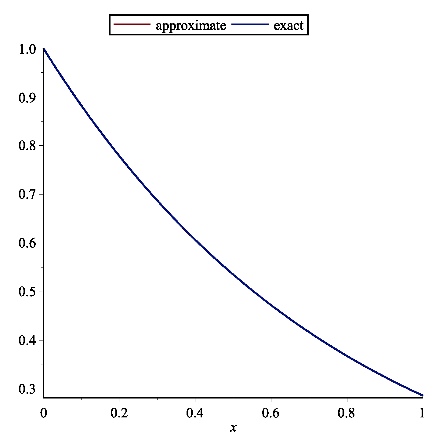
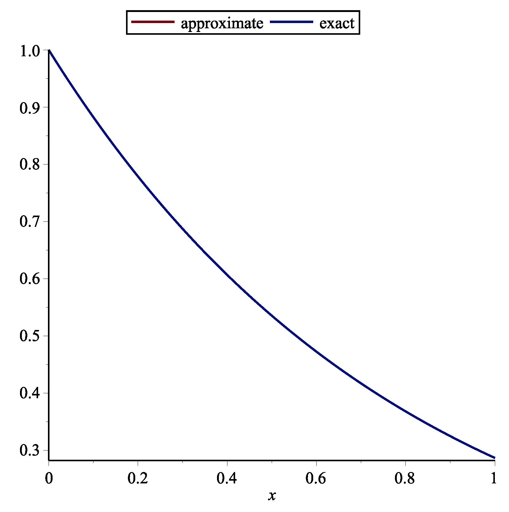
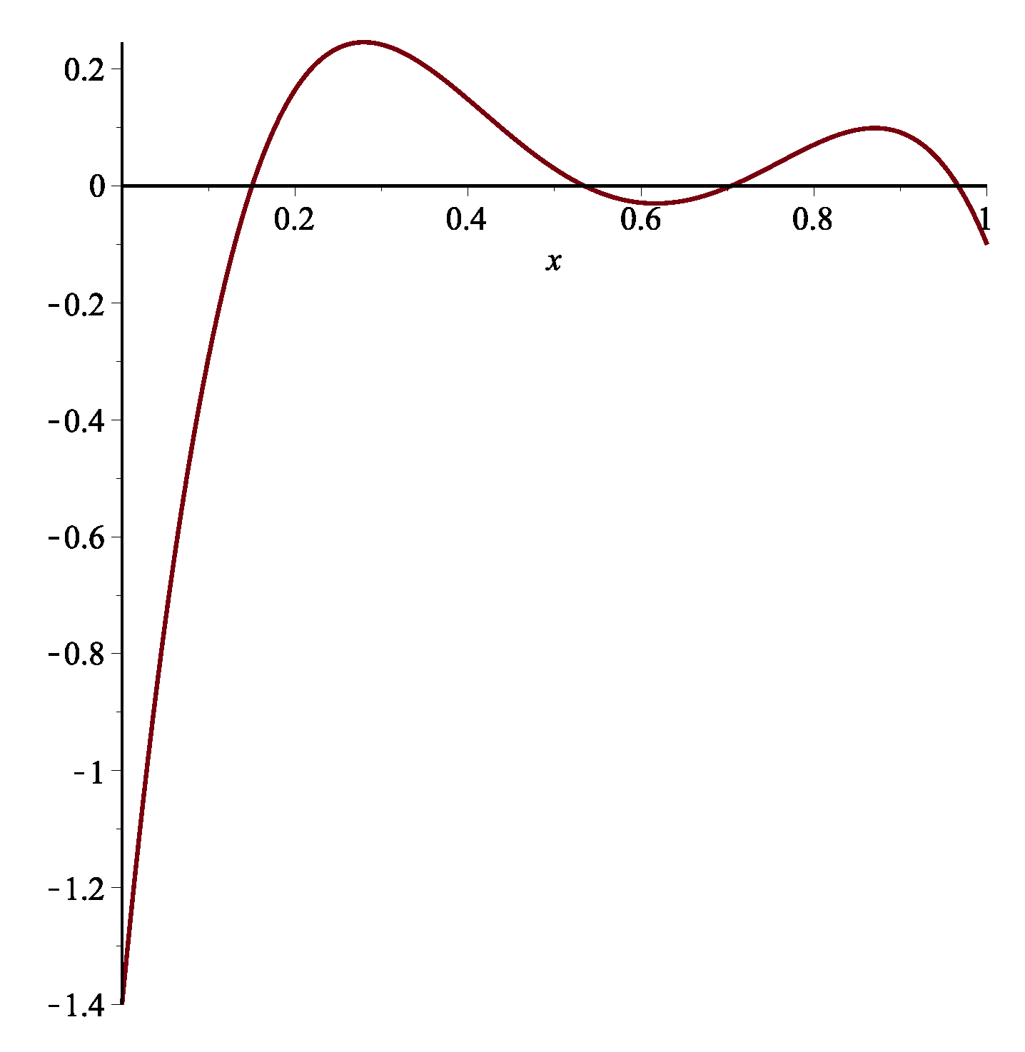
Example 1.

First, the following RDE is considered (see [15])

$$\begin{array}{c}{y}^{\prime }\left(x\right)=1+2y\left(x\right)-y^2\left(x\right),0\le x\le 1,\hfill \\ y\left(0\right)=1,\hfill \\ y_{exact}\left(x\right)=1+\sqrt{2}tanh\left(\sqrt{2}x+\frac{1}{2}log\left(\frac{\sqrt{2}-1}{\sqrt{2}+1}\right)\right),y_{exact}\left(0\right)=2\times {10}^{-10}\simeq 0.\hfill \end{array}$$

One may achieve $y_{approx}\left(x\right)=0.4836486196+1.959259361x+0.1873135074x^2-0.5349351716x^3$ with this technique by $n=4$. The approximate and exact solution for $y\left(x\right)$ are shown in Figure 1.

Table 1. The absolute error of the this method for Example 1.

x	Error of y
$0.1$	$0.01576255020$
$0.2$	$0.01957152970$
$0.3$	$0.01520160000$
$0.4$	$0.007259874300$
$0.5$	$7.000000000\times {10}^{-10}$
$0.6$	$0.003753795400$
$0.7$	$0.003263092300$
$0.8$	$3.000000000\times {10}^{-10}$
$0.9$	$0.002664043000$
$1.0$	$0.0$

demonstrates the absolute error of the this technique.

Example 2.

Second, the following RDE is considered (see [15])

$$\begin{array}{c}{y}^{\prime }\left(x\right)=16x^2-5+8xy\left(x\right)+y^2\left(x\right),0\le x\le 1,\hfill \\ y\left(0\right)=1,\hfill \\ y_{exact}\left(x\right)=1-4x,\hfill \end{array}$$

One may obtain $y_{approx}\left(x\right)=1-4x-2.864375404\times {10}^{-14}{x}^2+1.687538998\times {10}^{-14}{x}^3$ with this method by $n=4$. The approximate and exact solution for $y\left(x\right)$ are shown in Figure 2.

Table 2. The absolute error of the this method for Example 2.

x	Error of y for Presented Method	Error in [15]
$0.1$	$2.695621504\times {10}^{-16}$	$0.000233600365141$
$0.2$	$1.010747042\times {10}^{-15}$	$--$
$0.3$	$2.122302334\times {10}^{-15}$	$0.00045422294912$
$0.4$	$3.502975687\times {10}^{-15}$	$--$
$0.5$	$5.051514762\times {10}^{-15}$	$9.375\times {10}^{-11}$
$0.6$	$6.666667214\times {10}^{-15}$	$--$
$0.7$	$8.247180717\times {10}^{-15}$	$0.00045422275331$
$0.8$	$9.691802920\times {10}^{-15}$	$--$
$0.9$	$1.089928147\times {10}^{-14}$	$0.00023360043610$
$1.0$	$1.176836406\times {10}^{-14}$	$--$

demonstrates the absolute error of the this technique and stated technique in [15].

Example 3.

Third, the following RDE is considered (see [15])

$$\begin{array}{c}{y}^{\prime }\left(x\right)=16x^2-5+8xy\left(x\right)+y^2\left(x\right),0\le x\le 1,\hfill \\ y\left(0\right)=1,\hfill \\ y_{exact}\left(x\right)=1-4x,\hfill \end{array}$$

One may obtain $y_{approx}\left(x\right)=0.9999999998+1.026769538x+0.3911797260x^2+0.3003325646x^3$ with this method by $n=4$. The approximate and exact solutions for $y\left(x\right)$ are shown in Figure 3.

Table 3. The absolute error of the this method for Example 3.

x	Error of y
$0.1$	$0.001718166000$
$0.2$	$0.002000999000$
$0.3$	$0.001487207000$
$0.4$	$0.0006931570000$
$0.5$	$0.0$
$0.6$	$0.0003605420000$
$0.7$	$0.0003218950000$
$0.8$	$0.0$
$0.9$	$0.0002874910000$
$1.0$	$1.000000000\times {10}^{-9}$

demonstrates the absolute error of the this technique.

Remark 1.

Delay differential equations (DDEs) are defined as distributed delay systems. DDEs are encountered in various practical systems such as engineering, and in the modeling of feeding system (see [16]). Many researchers used various polynomials for solving DDEs. Orthogonal functions were utilized for solving OCSs with time delay ([17]). Also Chebyshev polynomials (ChPs) were used to solving time-varying systems with distributed time delay. The stated technique in [18] is based on expanding all time functions in terms of ChPs. The Bezier technique is utilized for solving DDEs and switched systems (see [15]). Using Bessel polynomials, pantograph equations were solved in [19].

Here, the following system of MPDDEs is considered

$$\begin{array}{c}{u}_1^{\prime }\left(x\right)={\beta }_1{u}_1\left(x\right)+f_1(x,u_1\left({\eta }_{11}x\right),\dots ,u_m\left({\eta }_{1m}x\right)),\hfill \\ u_2^{\prime }\left(x\right)={\beta }_2{u}_2\left(x\right)+f_2(x,u_1\left({\eta }_{21}x\right),\dots ,u_m\left({\eta }_{2m}x\right)),\hfill \\ ⋮\hfill \\ u_m^{\prime }\left(x\right)={\beta }_m{u}_m\left(x\right)+f_m(x,u_1\left({\eta }_{m1}x\right),\dots ,u_m\left({\eta }_{mm}x\right)),\hfill \\ u_i\left(x_0\right)=u_{i0},i=1,2,\dots ,m,x_0\le x\le x_f,x_0,x_f\in \mathcal{R},\hfill \\ 0<{\eta }_{ij}\le 1,i,j=1,2,\dots ,m,\hfill \end{array}$$

(8)

where $u_{i0}$ is given constant, $f_i$ and ${\beta }_i$ ($i=1,2,\dots ,m$) are given continuous functions.

MPDDEs are in various applications such as astrophysics, number theory, nonlinear dynamical systems (NDSs), quantum mechanics and cell growth, probability theory on algebraic structures, and etc. Properties of the analytic solution of MPDDEs as well as numerical techniques have been studied by several researchers. For example, there are treated in [20].

In this sequel, a new operational matrix of fractional order derivative based on GPs is introduced to provide approximate solutions of MPDDEs and optimal control systems with pantograph delays.

Our strategy is utilizing GPs to approximate the solution $u_i\left(x\right)$ by $u_i^N\left(x\right)$ is as given below.

$$\begin{array}{c}{u}_i\left(x\right)\approx u_i^N\left(x\right)=\sum _{n=1}^N{c}_n^i{G}_n\left(x\right)=G\left(x\right)C_i,\hfill \end{array}$$

where

$$\begin{array}{c}{C}_i^T=[c_1^i,c_2^i,\dots ,c_n^i],\hfill \end{array}$$

also $G\left(x\right)$ satisfies in Equations (4) and (5), then, the k-th derivative of $u_i\left(x\right)$ can be stated as

$$\begin{array}{c}\hfill u_i^{\left(k\right)}\left(x\right)=G^{\left(k\right)}\left(x\right)C_i=G\left(x\right){\left(M^T\right)}^k{C}_i,\end{array}$$

(9)

by Equations (8) and (6), we have

$$\begin{array}{c}G\left(x\right)M^T{C}_1={\beta }_{1}G\left(x\right)C_1+f_1(x,G\left({\eta }_{11}x\right)C_1,\dots ,G\left({\eta }_{1m}x\right)C_m),\hfill \\ G\left(x\right)M^T{C}_2={\beta }_{2}G\left(x\right)C_2+f_2(x,G\left({\eta }_{21}x\right)C_1,\dots ,G\left({\eta }_{2m}x\right)C_m),\hfill \\ ⋮\hfill \\ G\left(x\right)M^T{C}_m={\beta }_{m}G\left(x\right)C_m+f_m(x,G\left({\eta }_{m1}x\right)C_1,\dots ,G\left({\eta }_{mm}x\right)C_m),\hfill \\ G\left(x\right)C_i=u_{i0},i=1,2,\dots ,m,x_0\le x\le x_f,\hfill \\ 0<{\eta }_{ij}\le 1,i,j=1,2,\dots ,m,\hfill \end{array}$$

(10)

to obtain $u_i\left(x\right)$, one may use the collocation points $x_j=\frac{j-1}{N}$, $j=1,2,\dots ,N-1$.

5. Numerical Applications for Solving MPDDEs

In this section, some findings are given to demonstrate the quality of the sated technique in approximating the solution of MPDDEs and optimal control systems with pantograph delays.

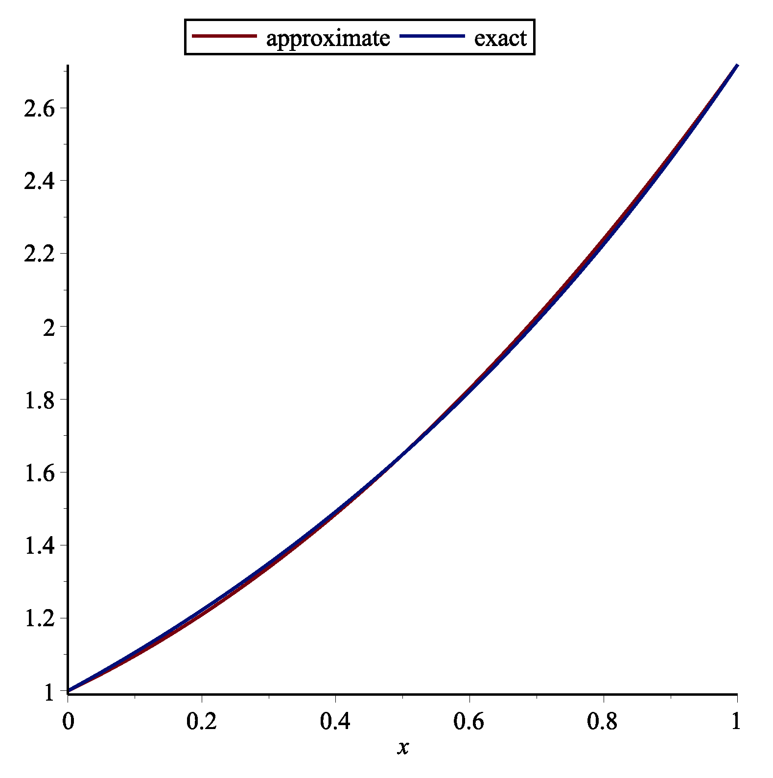
Example 4.

The following time-varying system described by (see [21])

$$\begin{array}{c}\frac{du}{dx}=-\frac{5}{4}{e}^{-\frac{1}{4}x}u\left(\frac{4}{5}x\right),0\le x\le 1,\hfill \\ u\left(0\right)=1,\hfill \\ u_{exact}\left(x\right)=e^{-1.25x},\hfill \end{array}$$

One may obtain

$$\begin{array}{ccc}\hfill u_{approx}\left(x\right)& =& 1-1.25x+0.775524733283677x^2\hfill \\ & -& 0.298896140751031x^3+0.0598762043673534x^4,\hfill \end{array}$$

with this method by $n=5$. The approximate and exact solution for $u\left(x\right)$ are shown in Figure 4.

Table 4. The absolute error of the this method for Example 4.

x	Error of $\mathit{u}\left(\mathit{x}\right)$
$0.1$	$0.3456378748\times {10}^{-4}$
$0.2$	$0.00007516096767$
$0.3$	$0.00007725134937$
$0.4$	$0.4322455087\times {10}^{-4}$
$0.5$	$5.551115123\times {10}^{-16}$
$0.6$	$0.2074096591\times {10}^{-4}$
$0.7$	$2.775557562\times {10}^{-16}$
$0.8$	$0.00005314265411$
$0.9$	$0.00008794236230$
$1.0$	$3.885780586\times {10}^{-16}$

demonstrates the absolute error of the this technique.

Example 5.

Consider the time-varying system described by (see [21])

$$\begin{array}{c}{u}^{\prime }\left(x\right)=-u\left(x\right)+0.1u\left(0.8x\right)+0.5x^{\prime }\left(0.8x\right)+(0.32x-0.5)e^{-0.8x}+e^{-x},\hfill \\ u\left(0\right)=1,\hfill \\ u_{exact}\left(x\right)=x{e}^x,\hfill \end{array}$$

One may obtain

$$\begin{array}{ccc}\hfill u_{approx}\left(x\right)& =& -1.11022302462516\times {10}^{-16}\hfill \\ & +& x-0.941756802771441x^2+0.309636243942884x^3,\hfill \end{array}$$

with this technique by $n=4$. The approximate and exact $u\left(x\right)$ are shown in Figure 5.

Example 6.

The following optimal control system with pantograph delay is considered (see [21])

$$\begin{array}{c}minI=\frac{1}{2}{\int }_0^1{u}_1^2\left(x\right)+u_2^2\left(x\right)dx,\hfill \\ s.t.\frac{d{u}_1}{dx}=u_1\left(0.5x\right)+4u_2\left(x\right),\hfill \\ u_1\left(0\right)=1,\hfill \end{array}$$

One may obtain

$$\begin{array}{ccc}\hfill u_{1,approx}\left(x\right)& =& -1.11022302462516\times {10}^{-16}\hfill \\ & +& x-0.941756802771441x^2+0.309636243942884x^3,\hfill \end{array}$$

with this technique by $n=5$. The approximate and exact $u_2\left(x\right)$ is shown in Figure 6.

Example 7.

First, the following two-dimensional pantograph equations is considered (see [22])

$$\begin{array}{c}{u}_1^{\prime }\left(x\right)-u_1\left(x\right)+u_2\left(x\right)-u_1\left(\frac{x}{2}\right)-f_1\left(x\right)=0,\hfill \\ u_2^{\prime }\left(x\right)+u_1\left(x\right)+u_2\left(x\right)+u_1\left(\frac{x}{2}\right)-f_2\left(x\right)=0,\hfill \\ f_1\left(x\right)=e^{-x}-e^{\frac{x}{2}},f_2\left(x\right)=e^x-e^{-\frac{x}{2}},\hfill \\ u_1\left(0\right)=1,u_2\left(0\right)=1,\hfill \\ u_{1,exact}\left(x\right)=e^x,\hfill \\ u_{2,exact}\left(x\right)=e^{-x},\hfill \end{array}$$

One may achieve

$$\begin{array}{ccc}\hfill u_{1,approx}\left(x\right)& =& 1+0.876603255540951x+0.841678572918099x^2,\hfill \\ \hfill u_{2,approx}\left(x\right)& =& 1-0.941756802371442x+0.309636243542884x^2,\hfill \end{array}$$

with this technique by $n=3$. The approximate and exact $u_{1,approx}\left(x\right)$ and $u_{2,appox}\left(x\right)$ are shown in Figure 7 and Figure 8.

Table 5. The absolute error of the this method for Example 7.

x	Error of ${\mathit{u}}_{1,\mathit{a}\mathit{p}\mathit{p}\mathit{r}\mathit{o}\mathit{x}}\left(\mathit{x}\right)$	Error of ${\mathit{u}}_{2,\mathit{a}\mathit{p}\mathit{p}\mathit{r}\mathit{o}\mathit{x}}\left(\mathit{x}\right)$
$0.2$	$0.01241496400$	$0.005303336200$
$0.4$	$0.006514824000$	$0.002519032000$
$0.6$	$0.006847440000$	$0.002396669800$
$0.8$	$0.01441596300$	$0.004567210100$
$1.0$	$0.0$	$0.0$

demonstrates the absolute error of the this technique.

6. Conclusions

In this paper, GPs stated for solving the RDEs, also GPs stated for solving the MPDDEs and optimal control systems with pantograph delays. The stated technique is computationally attractive. Some results are included to explain the validity of this technique. The presented approximate solutions are more accurate compared to the references as it is shown in the tables. By stated technique, the high orders of convergence obtained when it achieved accurate solutions even for small values of n.

References

- Reid, W.T. Riccati Differential Equations; Academic Press: NewYork, NY, USA, 1972. [Google Scholar]
- Dehghan, M.; Taleei, A. A compact split-step finite difference method for solving the nonlinear Schrödinger equations withconstant and variable coefficients. Comput. Phys. Commun. 2010, 181, 43–51. [Google Scholar] [CrossRef]
- Medina-Dorantes, F.I.; Villafuerte-Segura, R.; Aguirre-Hernández, B. Controller with time-delay to stabilize first-order procesases with dead-time. J. Control Eng. Appl. Inform. 2018, 20, 42–50. [Google Scholar]
- Villafuerte-Segura, R.; Medina-Dorantes, F.I.; Vite-Hernandez, L.; Aguirre-Hernández, B. Tuning of a time-delayed controller for a general clases of second-order LTI Systems with dead-time. IET Control Theory Appl. 2018, 13, 451–457. [Google Scholar] [CrossRef]
- Bulut, H.; Evans, D.J. On the solution of the Riccati equationby the decomposition method. Int. J. Comput. Math. 2002, 79, 103–109. [Google Scholar] [CrossRef]
- El-Tawil, M.A.; Bahnasawi, A.A.; Abdel-Naby, A. Solving Riccatidifferential equation using Adomian’s decomposition method. Appl. Math. Comput. 2004, 157, 503–514. [Google Scholar]
- Abbasbandy, S. Homotopy perturbation method for quadraticRiccati differential equation and comparison with Adomian’s decomposition method. Appl. Math. Comput. 2006, 172, 485–490. [Google Scholar]
- Geng, F.; Lin, Y.; Cui, M. A piecewise variational iteration methodfor Riccati differential equations. Comput. Math. Appl. 2009, 58, 2518–2522. [Google Scholar] [CrossRef]
- Mukherjee, S.; Roy, B. Solution of Riccati equation with variableco-efficient by differential transform method. Int. J. Nonlinear Sci. 2012, 14, 251–256. [Google Scholar]
- Isah, A.; Phang, C. Operational Matrix Based on Genocchi Polynomials for Solution of Delay Differential Equations. Ain Shams Eng. J. 2018, 9, 2123–2128. [Google Scholar] [CrossRef]
- Loh, J.R.; Phang, C. A New Numerical Scheme for Solving System of Volterra Integro-differential Equation. Alexandria Eng. J. 2018, 57, 1117–1124. [Google Scholar] [CrossRef]
- Afshan, K.; Phang, C.; Iqbal, U. Numerical Solution of Fractional Diffusion Wave Equation and Fractional Klein-Gordon Equation via Two-Dimensional Genocchi Polynomials with a Ritz-Galerkin Method. Computation 2018, 6, 40. [Google Scholar]
- Isah, A.; Phang, C. Operational matrix based on Genocchi polynomials for solution of delay differential equations. Ain Shams Eng. J. 2017. [Google Scholar] [CrossRef]
- Isah, A.; Phang, C. New operational matrix of derivative for solving non-linear fractional differential equations via Genocchi polynomials. J. King Saud Univ.-Sci. 2017. [Google Scholar] [CrossRef]
- Ghomanjani, F.; Khorram, E. Approximate solution for quadratic Riccati differential equation. J. Taibah Univ. Sci. 2017, 11, 246–250. [Google Scholar] [CrossRef]
- Chen, W.; Zheng, W.X. Delay-dependent robust stabilization for uncertain neutral systemswith distributed delays. Automatica 2007, 43, 95–104. [Google Scholar] [CrossRef]
- Nazarzadeh, J. Finite Time Nonlinear Optimal Systems Solution by Spectral Methods. Ph.D. Thesis, Amirkabir University of Technology, Tehran, Iran, 1998. [Google Scholar]
- Esfanjani, R.M.; Nikravesh, S.K.Y. Predictive control for a class of distributed delay systems using Chebyshev polynomials. Int. J. Comput. Math. 2010, 87, 1591–1601. [Google Scholar] [CrossRef]
- Yüzbasi, S.; Sahin, N.; Sezar, M. A Bessel collocation method for numerical solution of generalized pantograph equations. Numer. Methods Part. Equ. 2012, 28, 1105–1123. [Google Scholar] [CrossRef]
- Derfel, G.A.; Vogl, F. On the asymptotics of solutions of a class of linear functional-differential equations. Eur. J. Appl. Math. 1996, 7, 511–518. [Google Scholar] [CrossRef]
- Ghomanjani, F.; Farahi, M.H.; Kamyad, A.V. Numerical solution of some linear optimal control systems with pantograph delays. IMA J. Math. Control Inf. 2015, 32, 225–243. [Google Scholar] [CrossRef]
- Komashynska, I.; Al-Smadi, M.; Al-Habahbeh, A.; Ateiwi, A. Analytical approximate solutions of systems of multi-pantograph delay differential equations using residual power-series method. Aust. J. Basic Appl. Sci. 2014, 8, 664–675. [Google Scholar]
© 2020 by the authors. Licensee MDPI, Basel, Switzerland. This article is an open access article distributed under the terms and conditions of the Creative Commons Attribution (CC BY) license (http://creativecommons.org/licenses/by/4.0/).