Approximate Methods for Solving Linear and Nonlinear Hypersingular Integral Equations

Abstract

We propose an iterative projection method for solving linear and nonlinear hypersingular integral equations with non-Riemann integrable functions on the right-hand sides. We investigate hypersingular integral equations with second order singularities. Today, hypersingular integral equations of this type are widely used in physics and technology. The convergence of the proposed method is based on the Lyapunov stability theory of solutions of ordinary differential equation systems. The advantage of the method for linear equations is in simplicity of unique solvability verification for the approximate equations system in terms of the operator logarithmic norm. This makes it possible to estimate the norm of the inverse matrix for an approximating system. The advantage of the method for nonlinear equations is that neither the existence or reversibility of the nonlinear operator derivative is required. Examples are given illustrating the effectiveness of the proposed method.

1. Introduction

The importance of developing analytical and numerical methods for solving hypersingular integral equations is determined by a variety of fields of mathematics and by applications that use hypersingular integral equations.

Hadamard introduced the concept of a finite part of an integral, or the hypersingular integral in modern terminology, when studying hyperbolic equations. The Riemann boundary problem leads to hypersingular integral equations in exceptional cases. The boundary integral equations method reduces the dimensions of partial differential equations; that leads to hypersingular integral equations.

Hypersingular integral equations, singular integral equations and Riemann boundary problem are widely used in aerodynamics, electrodynamics, quantum physics, antennae theory and many other fields of physics and engineering [1,2,3,4,5].

Analytical methods for solving singular and hypersingular integral equations are known only for certain particular types of equations [6,7,8]. Thus, the importance of constructing numerical solutions is clear.

Developing numerical methods for solving singular integral equations began in the middle of the last century. By now, exhaustive results have been obtained for many types of equations. A detailed account of numerical methods for solving singular integral equations as well as numerous bibliography references can be found in [9,10,11,12,13,14].

Numerical methods for solving hypersingular integral equations have been developed to a much lesser extent. Mostly numerical methods to solve hypersingular integral equations of the first kind have been developed. Numerical methods for solving hypersingular integral equations of the second kind have been much less developed. Apparently, hypersingular integral equations of the first kind are more common. Naturally, the equations of the first kind are widely used in aerodynamics (one-dimensional [15] and multi-dimensional [5,16] Prandtl equation), electrodynamics, antennae theory, etc.

The following methods are used in solving hypersingular integral equations of the first kind.

Collocations, mechanical quadratures and Galerkin methods were employed to solve equations with p = 2 singularity [6,17,18,19].

Approximate methods for solving hypersingular integral equations having singularities of order $p=2,3,\dots ,$ and defined on closed smooth integration contours are constructed in [20].

In [21,22] spline-collocation methods for solving hypersingular and polyhypersingular integral equations of the second kind with odd and even singularities have been developed and justified. The spline-collocation methods for solving nonlinear hypersingular and polyhypersingular integral equations have been developed and justified in [23].

An iterative projection method for solving linear and nonlinear hypersingular integral equations, and polyhyperpersingular and multidimensional hypersingular equations, was proposed in [24].

In [22] the unique solvability of hypersingular integral equations with even singularities (p = 2, 4, …) was proven. Meanwhile the convergence of approximate solution to the exact one was not justified. In [24] a unique solvability of the spline-collocation method was proven. In addition, for hypersingular integral equations with bounded right-hand sides the convergence of an approximate solution sequence to the exact solution was proven under certain additional conditions.

The iterative projection method proposed here overcomes these limitations. It was shown that if the exact equation has a solution for large enough N, where N is the dimension of an approximate system of equations, an approximate solution converges to the exact one.

Hypersingular integral equations with bounded right-hand sides are a small subset of the hypersingular integral equations family. Therefore, the problem arises of constructing and justifying approximate methods for solutions for hypersingular integral equations with non-Riemann integrable functions on the right-hand sides. This paper is devoted to those issues.

A large number of works are devoted to approximate methods for solving hypersingular integral equations of the first kind

$$\underset{-1}{\overset{1}{\int }}\frac{x(\tau )d\tau }{{(\tau -t)}^2}+\underset{-1}{\overset{1}{\int }}h(t,\tau )d\tau =f(t).$$

(1)

To solve the Equation (1), collocation and mechanical quadrature methods [17,18], the method of orthogonal polynomials [25], the method of discrete vortices [19], the method of homotopy [26] and others are used.

In the works [27,28,29] computational schemes for the approximate solution of the Equation (1) are constructed and their justification is carried out under the assumption that the solution has the forms $x(t)={(1-t^2)}^{\pm 1/2}\omega (t)$ or $x(t)={((1-t)/(1+t))}^{\pm 1/2}\omega (t)$, where $\omega (t)$ is a smooth function.

The hypersingular integral equations

$$\frac{1}{\pi }\underset{-1}{\overset{1}{\int }}\frac{x(\tau )d\tau }{{(\tau -t)}^2}=f(t),-1<t<1,$$

(2)

are widely used in aerodinamical problems and in the theory of antennae [30,31]. In the works [30,31] the Equation (2) is investigated under the assumption that the right-hand side has the form $f(t)=1/(t-c)$ or $f(t)=\delta (t-c)$, where $\delta (t)$ is the delta-function. An analytical solution of the Equation (2) with the indicated right-hand sides is obtained under the assumption that it has the form $x(t)=\sqrt{1-t^2}\phi (t).$

A fairly detailed review of analytical and numerical methods for solving hypersingular integral equations is given in [32].

In this paper, we propose an approach to solving linear and nonlinear hypersingular integral equations, the right parts of which contain functions with power features.

In particular, the right-hand sides of the form

$$f(t)=g(t)\frac{1}{t-c_1}\frac{1}{t-c_2}\cdots \frac{1}{t-c_l},l=1,2,\dots ,-1<c_1<\cdots <c_l<1,$$

(3)

are considered. Here $g(t)$ is a smooth function.

Below, for simplicity of notation, we put $l=1$ in (3).

Remark 1.

It can be shown that if in the hypersingular integral Equation (1) of the first kind the right side $f(t)\in H$, H is a Holder class, then the solution to this equation has the form $x(t)={(1-t^2)}^{\pm 1/2}$ or $x(t)={((1+t)/(1-t))}^{\pm 1/2}$. For singular right-hand sides, the classes of solutions of (1) are unknown.

Below, when constructing and justifying the computational method, we assume that the Equation (1) with a given right-hand side has a unique solution.

The proposed method has the following advantages:

(1)

It allows us to extend collocations and mechanical quadratures methods to hypersingular integral equations with non-Riemann integrable right sides;

(2)

For linear hypersingular integral equations, it allows one to verify the inverse operator existence and estimate its norm quite easily;

(3)

The method is stable with respect to the operator and right hand side perturbations;

(4)

The method does not require the existence and reversibility of the nonlinear operator derivative.

The paper is organized as follows. The continuous method for linear and nonlinear operator equations is explained in Section 2. The numerical method for solving hypersingular integral equations is presented in Section 2.

2. Continuous Method and Its Convergence Properties

The method we employ in the next section for solving hypersingular integral equations is based on the continuous method introduced in [33].

Continuous Method for Solving Operator Equations

The continuous method for solving operator equations is based on the Lyapunov theory of stability.

Let $x(t)$ be a solution of the differential equation in a Banach space B

$$\frac{dx}{dt}=F(t,x)$$

(4)

which is defined for all $t\ge t_0$. The solution $x(t)$ is said to be stable if (i) for each $\epsilon >0$ there is a corresponding $\delta =\delta (\epsilon )>0$ such that any solution $\tilde{x}(t)$ of (4) which satisfies the inequality $|\tilde{x}(t_0)-x(t_0)|<\delta$ exists and satisfies the inequality $|\tilde{x}(t)-x(t)|<\epsilon$ for all $t\ge t_0$.

It is said to be asymptotically stable if in addition (ii) $|\tilde{x}(t)-x(t)|\to 0$ if $t\to \infty$ whenever $|\tilde{x}(t_0)-x(t_0)|$ is sufficiently small.

We will use the following notation:

$$\begin{gathered} B(a,r)=\{z\in B:\parallel z-a\parallel \le r\},S(a,r)=\{z\in B:\parallel z-a\parallel =r\},Re(K)=\Re (K)=(K+K^{\ast })/2 \\ \Lambda (K)=\underset{h\downarrow 0}{lim}(\parallel I+hK\parallel -1)h^{-1} \end{gathered}$$

.

Here B is a Banach space, $a\in B$, K is a linear operator on B, $\Lambda (K)$ is the logarithmic norm [34] of the operator K, $K^{\ast }$ is the conjugate operator to K and I is the identity operator.

The analytical expressions for logarithmic norms are known for operators in many spaces. We restrict ourselves to a description of the three norms.

Let $A=\left\{a_{ij}\right\}$, $i,j=1,2,\dots ,n$, be a matrix.

In the n-dimensional space $R_n$ of vectors $x=(x_1,\dots ,x_n)$ the following norms are often used:

$$\begin{gathered} \mathrm{octahedral}-{\parallel x\parallel }_1=\sum _{i=1}^n\left|x_i\right|;\mathrm{cubic}-{\parallel x\parallel }_2=\underset{1\le i\le n}{max}\left|x_i\right|; \\ \mathrm{spherical} (\mathrm{Euclidean})-{\parallel x\parallel }_3={(\sum _{i=1}^n{x}_i^2)}^{1/2}. \end{gathered}$$

Here are analytical expressions of the logarithmic norm of $n\times n$ matrix $A=(a_{ij}),$ due to the above norms of the vectors:

octahedral logarithmic norm ${\Lambda }_1$

$${\Lambda }_1(A)=\underset{1\le j\le n}{max}\left(a_{jj}+\sum _{i\ne j}\left|a_{ij}\right|\right);$$

cubic logarithmic norm ${\Lambda }_2$

$${\Lambda }_2(A)=\underset{1\le i\le n}{max}\left(a_{ii}+\sum _{j\ne i}\left|a_{ij}\right|\right);$$

spherical (Euclidean) logarithmic norm ${\Lambda }_3$

$${\Lambda }_3(A)={\lambda }_{max}\left(\frac{A+A^{\ast }}{2}\right),$$

where $A^{\ast }$ is the conjugate matrix for $A.$

Note that the logarithmic norm of the same matrix can be positive in one space and negative in another.

The logarithmic norm has the some properties which are very useful for numerical mathematics.

Let $A,B$ be $n\times n$ matrices with complex elements; and $x=(x_1,\dots ,x_n)$, $y=(y_1,\dots ,y_n)$, $\xi =({\xi }_1,\dots ,{\xi }_n)$ and $\eta =({\eta }_1,\dots ,{\eta }_n)$ are n-dimensional vectors with complex components. Let the systems of algebraic equations $Ax=\xi$ and $By=\eta$ be given. The norm of a vector and its subordinate operator norm of the matrix are agreed upon; the logarithmic norm $\Lambda (A)$ corresponds to the operator norm.

Theorem 1

([35]). If $\Lambda (A)<0$, the matrix A is non-singular and $\parallel A^{-1}\parallel \le 1/|\Lambda (A)|$.

Theorem 2

([35]). Let $Ax=\xi$, $By=\eta$ and $\Lambda (A)<0$, $\Lambda (B)<0$. Then

$$\parallel x-y\parallel \le \frac{\parallel \xi -\eta \parallel }{|\Lambda (B)|}+\frac{\parallel A-B\parallel }{|\Lambda (A)\Lambda (B)|}.$$

Some properties of the logarithmic norm in a Banach space, which are useful in numerical mathematics, are given in [34].

Let us consider in a Banach space B, the Cauchy problem

$$\frac{dx(t)}{dt}=A(x(t)),$$

(5)

$$x(0)=x_0.$$

(6)

Let us assume that the nonlinear operator A has a Frechet derivative and $A(0)=0$.

The sufficiently satisfying conditions of asymptotically stability for the solution of the Cauchy problem (5), (6) were obtained in [36,37].

Theorem 3.

Let the integral $\underset{0}{\overset{t}{\int }}\Lambda (A^{\prime }(\phi (\tau )))d\tau$ be non-positive (respectively, be negative and satisfy $\underset{t\to +\infty }{lim}\frac{1}{t}\underset{0}{\overset{t}{\int }}\Lambda (A^{\prime }(\phi (\tau )))d\tau \le -{\alpha }_{\phi },{\alpha }_{\phi }>0$) for any differentiable curve $\phi (t)$ lying in a ball $B(0,r)$ of some radius r. Then the trivial solution of Equation (5) is stable (respectively, asymptotically stable).

Remark 2.

Additionally, the Theorem is valid under $r=\infty$.

Let us consider in a Banach space B a nonlinear operator equation

$$A(x)-f=0,$$

(7)

where operator A acts from B into B.

We associate Equation (7) with the Cauchy problem

$$\frac{dx(t)}{dt}=A(x(t))-f,$$

(8)

$$x(0)=x_0.$$

(9)

Let $x^{\ast }$ be a the solution of Equation (7). Let us make the change of variable $x=x^{\ast }+v$ in Equation (8). This change reduces the Cauchy problem (8), (9) to the form

$$\frac{dv(t)}{dt}=A(x^{\ast }+v(t))-A(x^{\ast }),$$

(10)

$$v(0)=x_0-x^{\ast }.$$

(11)

It is easy to see that if the trivial solution of Equation (10) is globally asymptotically stable, then ${lim}_{t\to +\infty }\parallel v(t)\parallel \to 0$. So, for any initial value the solution of the Cauchy problem (8), (9) tends to $x^{\ast }$. It follows from the next assertions which were proven in [33].

Theorem 4.

Let $Equation(7)$ have a solution $x^{\ast }$, and let inequality

$$\underset{t\to +\infty }{lim}\frac{1}{t}\underset{0}{\overset{t}{\int }}\Lambda (A^{\prime }(g(\tau )))d\tau \le -{\alpha }_g,{\alpha }_g>0,$$

(12)

be true on each differentiable curve $g(t)$ lying in the Banach space B. Then the solution of the Cauchy problem (8), (9) converges to the solution $x^{\ast }$ of $Equation(7)$ for any initial value.

Theorem 5.

Let Equation (7) have a solution $x^{\ast }$, and let the following conditions be satisfied on any differentiable curve $g(t)$ lying in the ball $B(x^{\ast },r)$.

1.

The inequality

$$\underset{0}{\overset{t}{\int }}\Lambda (A^{\prime }(g(\tau )))d\tau \le 0$$

holds for all $t(t>0)$.

2.

Inequality (12) is satisfied.

Then the solution of the Cauchy problem (8), (9) converges to the solution $x^{\ast }$ of Equation (7).

Remark 3.

The sufficient condition for convergence of the Cauchy problem (8), (9) solution to the solution of the operator Equation (7) is given above. It was obtained by analysing Lyapunov stability. One of the first basic results in accretive operator theory was a relation between the solution of operator equation $Au=0$, where A is a locally Lipschitzian and accretive operator, and the differential equation $\frac{du}{dt}=Au$ was obtained in [38].

Later, accretive operator theory and its applications for finding fixed points and constructing iterative procedures were studied by many authors. Basic results and a detailed bibliography devoted to the subject may be found in [39,40,41,42].

3. An Solution of Hypersingular Integral Equations with the Continuous Method

Let us consider the method of mechanical quadrature for solving hypersingular integral equation of the types

$$a(t)x(t)+{\int }_{-1}^1\frac{h(t,\tau )x(\tau )d\tau }{{(\tau -t)}^2}=f(t).$$

(13)

and

$$a(t)x(t)+{\int }_{-1}^1\frac{h(t,\tau ,x(\tau ))d\tau }{{(\tau -t)}^2}=f(t).$$

(14)

It is assumed that in the Equations (13) and (14) the right-hand sides have features of the following types

$$\begin{array}{c}f(t)=\sum _{i=1}^l{g}_i(t)\frac{1}{t-c_i},f(t)=g(t)\prod _{i=1}^l\frac{1}{t-c_i},\end{array}$$

where $-1<c_i<1,i=1,2,\dots ,l,l=1,2,\dots ;g(t),g_i(t),i=1,2,\cdots ,l,$—are continuous functions.

In what follows, without loss of generality, we set $l=1.$

Let us recall the Hadamard definition of hypersingular integrals [43].

Definition 1

([43]). The integral of the type

$${\int }_a^b\frac{A(x)dx}{{(b-x)}^{p+\alpha }}$$

for an integer p and $0<\alpha <1$, is defined as

$$\underset{x\to b}{lim}\left[{\int }_a^x\frac{A(t)dt}{{(b-t)}^{p+\alpha }}+\frac{B(x)}{{(b-x)}^{p+\alpha -1}}\right],$$

if $A(x)$ has p derivatives in the neighborhood of the point b. Here $B(x)$ is any function that satisfies the following two conditions:

(i) 

The above limit exists;

(ii) 

$B(x)$ has at least p derivatives in the neighborhood of the point $x=b$.

It is easy to see [43], that the conditions (i) and (ii) are sufficient for the existence of the limit.

Chikin in [44] introduced the following definition.

Definition 2

([44]). The Cauchy–Hadamard principal value of the integral

$${\int }_a^b\frac{\phi (\tau )d\tau }{{(\tau -c)}^p},a<c<b,$$

(15)

is defined as

$${\int }_a^b\frac{\phi (\tau )d\tau }{{(\tau -c)}^p}=\underset{v\to 0}{lim}\left[{\int }_a^{c-v}\frac{\phi (\tau )d\tau }{{(\tau -c)}^p}+{\int }_{c+v}^b\frac{\phi (\tau )d\tau }{{(\tau -c)}^p}+\frac{\xi (v)}{v^{p-1}}\right],$$

where $\xi (v)$ is a function constructed so that the limit exists.

3.1. An Approximate Solution of Linear Hypersingular Integral Equations with Second Order Singularity

Consider a one-dimensional hypersingular integral equation of the type

$$Kx\equiv a(t)x(t)+{\int }_{-1}^1\frac{h(t,\tau )x(\tau )d\tau }{{(\tau -t)}^2}=f(t),$$

(16)

where $f(t)=g(t)/(t-c)$ or $f(t)=g(t)/((1-t^2)(t-c)),-1<c<1,g(t)\in C[-1,1].$

Divide the interval $[-1,1]$ into two subintervals $[-1,c]$, $[c,1]$.

Let us fix a positive integer $N_0$. Put $h=2/N_0,N_1=\lceil (1+c)/h\rceil ,N_2=\lceil (1-c)/h\rceil ,N=N_1+N_2.$

Divide the interval $[-1,c]$ into $N_1$ subintervals at the points $t_k=-1+(c+1)k/N_1,$ $k=0,1,\dots ,N_1$.

Divide the interval $[c,1]$ into $N_2$ subintervals at the points ${\tau }_k=c+(1-c)k/N_2,$ $k=0,1,\dots ,N_2$.

Let us introduce the nodes ${\overline{t}}_0=t_0+1/2{(N_1)}^2,{\overline{t}}_k=t_k,k=1,2,\dots ,N_1-1,{\overline{t}}_{N_1}=t_{N_1}-1/2{(N_1)}^2;{\overline{\tau }}_0={\tau }_0+1/2{(N_2)}^2,{\overline{\tau }}_k={\tau }_k,k=1,2,\dots ,N_2-1,{\overline{\tau }}_{N_2}=1-1/2{(N_2)}^2$.

As an approximate solution of (16), we shall seek in the form of a continuous function

$$x_N(t)=\sum _{k=0}^{N_1}{\alpha }_k{\phi }_k(t)+\sum _{k=0}^{N_2}{\beta }_k{\psi }_k(t),$$

(17)

where ${\phi }_k(t),k=0,1,\dots ,N_1$, ${\psi }_k(t),k=0,1,\dots ,N_2$ is a family of basis functions.

For nodes $t_k,$ $k=1,\dots ,N_1-1,$ the corresponding basis elements are determined by

$${\phi }_k(t)=\left\{\begin{array}{cc}0,\hfill & t_{k-1}\le t\le t_{k-1}+\frac{1}{N_1^2},\hfill \\ \frac{N_1^2}{(1+c)N_1-2}(t-t_{k-1})-\frac{1}{(1+c)N_1-2},\hfill & t_{k-1}+\frac{1}{N_1^2}\le t\le t_k-\frac{1}{N_1^2},\hfill \\ 1,\hfill & t_k-\frac{1}{N_1^2}\le t\le t_k+\frac{1}{N_1^2},\hfill \\ -\frac{N_1^2}{(1+c)N_1-2}(t-t_k-\frac{1}{N_1^2})+1,\hfill & t_k+\frac{1}{N_1^2}\le t\le t_{k+1}-\frac{1}{N_1^2},\hfill \\ 0,\hfill & t_{k+1}-\frac{1}{N_1^2}\le t\le t_{k+1},\hfill \\ 0,\hfill & t\in [-1,1]\backslash [t_{k-1},t_{k+1}].\hfill \end{array}\right.$$

(18)

For boundary nodes $t_k,$ $k=0$ and $k=N_1$ the corresponding basis elements are defined as

$${\phi }_0(t)=\left\{\begin{array}{cc}1,\hfill & -1\le t\le -1+\frac{1}{N_1^2},\hfill \\ -\frac{N_1^2}{(1+c)N_1-2}(t+1-\frac{1}{N_1^2})+1,\hfill & -1+\frac{1}{N_1^2}\le t\le t_1-\frac{1}{N_1^2},\hfill \\ 0,\hfill & t_1-\frac{1}{N_1^2}\le t\le t_1,\hfill \\ 0,\hfill & [-1,1]\backslash [t_0,t_1];\hfill \end{array}\right.$$

(19)

and

$${\phi }_{N_1}(t)=\left\{\begin{array}{cc}0,\hfill & -1\le t\le t_{N_1-1}+\frac{1}{N_1^2},\hfill \\ \frac{N_1^2}{(1+c)N_1-2}(t-t_{N_1-1})-\frac{1}{(1+c)N_1-2},\hfill & t_{N_1-1}+\frac{1}{N_1^2}\le t\le c-\frac{1}{N_1^2},\hfill \\ 1,\hfill & c-\frac{1}{N_1^2}\le t\le c.\hfill \end{array}\right.$$

(20)

For nodes ${\tau }_k,$ $k=0,1,\dots ,N_2,$ the corresponding basis elements ${\psi }_k,k=0,1,\dots ,N_2,$ are determined in a the similar way: For nodes ${\tau }_k,$ $k=1,\dots ,N_2-1,$ the corresponding basis elements are determined by

$${\psi }_k(t)=\left\{\begin{array}{cc}0,\hfill & {\tau }_{k-1}\le t\le {\tau }_{k-1}+\frac{1}{N_2^2},\hfill \\ \frac{N_2^2}{(1-c)N_2-2}(t-{\tau }_{k-1})-\frac{1}{(1-c)N_2-2},\hfill & {\tau }_{k-1}+\frac{1}{N_2^2}\le t\le {\tau }_k-\frac{1}{N_2^2},\hfill \\ 1,\hfill & {\tau }_k-\frac{1}{N_2^2}\le t\le {\tau }_k+\frac{1}{N_2^2},\hfill \\ -\frac{N_2^2}{(1-c)N_2-2}(t-{\tau }_k-\frac{1}{N_2^2})+1,\hfill & {\tau }_k+\frac{1}{N_2^2}\le t\le {\tau }_{k+1}-\frac{1}{N_2^2},\hfill \\ 0,\hfill & {\tau }_{k+1}-\frac{1}{N_2^2}\le t\le {\tau }_{k+1},\hfill \\ 0,\hfill & t\in [-1,1]\backslash [{\tau }_{k-1},{\tau }_{k+1}].\hfill \end{array}\right.$$

(21)

For boundary nodes ${\tau }_k,$ $k=0$ and $k=N_2$ the corresponding basis elements are defined as

$${\psi }_0(t)=\left\{\begin{array}{cc}1,\hfill & c\le t\le c+\frac{1}{N_1^2},\hfill \\ -\frac{N_2^2}{(1-c)N_2-2}(t-c-\frac{1}{N_2^2})+1,\hfill & c+\frac{1}{N_2^2}\le t\le {\tau }_1-\frac{1}{N_2^2},\hfill \\ 0,\hfill & {\tau }_1-\frac{1}{N_2^2}\le t\le {\tau }_1,\hfill \\ 0,\hfill & [-1,1]\backslash [c,{\tau }_1];\hfill \end{array}\right.$$

(22)

and

$${\psi }_{N_2}(t)=\left\{\begin{array}{cc}0,\hfill & -1\le t\le {\tau }_{N_2-1}+\frac{1}{N_2^2},\hfill \\ \frac{N_2^2}{(1-c)N_2-2}(t-{\tau }_{N_2-1})-\frac{1}{(1-c)N_2-2},\hfill & {\tau }_{N_2-1}+\frac{1}{N_2^2}\le t\le 1-\frac{1}{N_2^2},\hfill \\ 1,\hfill & 1-\frac{1}{N_2^2}\le t\le 1.\hfill \end{array}\right.$$

(23)

To simplify the description of computational scheme, we introduce the following notation:

(1)

Unite the nodes $t_k,k=0,1,\dots ,N_1$ and ${\tau }_l,l=0,1,\dots ,N_2$, denoting them by $v_i,i=0,1,\dots ,N^{\ast },N^{\ast }=N_1+N_2;$

(2)

Unite the nodes ${\overline{t}}_k,k=0,1,\dots ,N_1$ and ${\overline{\tau }}_l,l=0,1,\dots ,N_2$, denoting them by ${\overline{v}}_i,i=0,1,\dots ,N^{\ast }+1;$

(3)

Denote the family of basis functions $\left\{{\phi }_k\right\},k=0,1,\dots ,N_1$ , $\left\{{\psi }_l\right\},l=0,1,\dots ,N_2$ by $\left\{{\zeta }_j\right\},j=0,1,\dots ,N^{\ast }+1$;

(4)

Denote by $\left\{{\gamma }_k\right\},k=0,1,\dots ,N^{\ast }+1,$ unknowns $\left\{{\alpha }_i\right\},i=0,1,\dots ,N_1$ , $\left\{{\beta }_j\right\},j=0,1,\dots ,N_2$.

Here $v_i=t_i,i=0,1,\dots ,N_1$ , $v_{N_1+i}={\tau }_i,i=1,2,\dots ,N_2$,

${\gamma }_i={\alpha }_i,i=0,1,\dots ,N_1$ , ${\gamma }_{N_1+1+i}={\beta }_i,i=0,1,\dots ,N_2,$

${\zeta }_i={\phi }_i,i=0,1,\dots ,N_1$ , ${\zeta }_{N_1+1+i}={\psi }_i,i=0,1,\dots ,N_2.$

Let us recall that the points $t_{N_1}$ and ${\tau }_0$ coincide.

Applying the collocation method on the knots ${\overline{v}}_k,k=0,1,\dots ,N^{\ast }+1$ to the Equation (16), we obtain the following system of algebraic equations for finding unknown coefficients $\left\{{\gamma }_k\right\}$ of the polygon (17)

$$a({\overline{v}}_k){\gamma }_k+\sum _{l=0}^{N^{\ast }+1}h({\overline{v}}_k,v_l){\gamma }_l\underset{-1}{\overset{1}{\int }}\frac{{\zeta }_l(\tau )}{{(\tau -{\overline{v}}_k)}^2}d\tau =f({\overline{v}}_k),$$

(24)

$k=0,1,\dots ,N^{\ast }+1.$

Using the definition of hypersingular integrals, we receive:

$$\underset{v_{k-1}}{\overset{v_{k+1}}{\int }}\frac{{\zeta }_k(\tau )d\tau }{{(\tau -{\overline{v}}_k)}^2}=-2\frac{N_1^2}{(1+c)N_1-2}ln((1+c)N_1-1),k=1,2,\dots ,N_1-1;$$

(25)

$$\underset{v_{k-1}}{\overset{v_{k+1}}{\int }}\frac{{\zeta }_{k+1}(\tau )d\tau }{{(\tau -{\overline{v}}_k)}^2}=-2\frac{N_2^2}{(1-c)N_2-2}ln((1-c)N_2-1),k=N_1+2,\dots ,N^{\ast }-1;$$

(26)

$$\underset{-1}{\overset{v_1}{\int }}\frac{{\zeta }_0(\tau )d\tau }{{(\tau +1-\frac{1}{2N_1^2})}^2}=-2N_1^2-N_1^2\frac{ln(2(c+1)N_1-3)}{(c+1)N_1-2},$$

(27)

$$\underset{v_{N_1-1}}{\overset{v_{N_1}}{\int }}\frac{{\zeta }_{N_1}(\tau )d\tau }{{(\tau -v_{N_1}+\frac{1}{2N_1^2})}^2}=-2N_1^2-N_1^2\frac{ln(2(c+1)N_1-3)}{(c+1)N_1-2},$$

(28)

$$\underset{v_{N_1}}{\overset{v_{N_1+1}}{\int }}\frac{{\zeta }_{N_1+1}(\tau )d\tau }{{(\tau -v_{N_1}-\frac{1}{2N_2^2})}^2}=-2N_2^2-N_2^2\frac{ln(2(1-c)N_2-3)}{(1-c)N_2-2},$$

(29)

$$\underset{v_{N^{\ast }-1}}{\overset{1}{\int }}\frac{{\zeta }_{N^{\ast }+1}(\tau )d\tau }{{(\tau -1+\frac{1}{2N^2})}^2}=-2N_2^2-N_2^2\frac{ln(2(1-c)N_2-3)}{(1-c)N_2-2},$$

(30)

$$\underset{-1}{\overset{1}{\int }}\left[\sum _{l=1}^{N^{\ast }+1}{\zeta }_l(\tau )\right]\frac{d\tau }{{(\tau +1-\frac{1}{2N_1^2})}^2}=-\frac{2N_1^2}{4N_1^2-1}+N_1^2\frac{ln(2(1+c)N_1-3)}{(1+c)N_1-2},$$

(31)

$$\underset{-1}{\overset{1}{\int }}\left[\sum _{l=0}^{N^{\ast }}{\zeta }_l(\tau )\right]\frac{d\tau }{{(\tau -1+\frac{1}{2N_2^2})}^2}=-\frac{2N_2^2}{4N_2^2-1}+N_2^2\frac{ln(2(1-c)N_2-3)}{(1-c)N_2-2},$$

(32)

$$\underset{-1}{\overset{1}{\int }}\left[\sum _{l=0}^{N^{\ast }+1}{}^{\prime }{\zeta }_l(\tau )\right]\frac{d\tau }{{(\tau -(c-\frac{1}{2N_1^2}))}^2}=-\frac{2N_1^2}{4N_1^2-1}+N_1^2\frac{ln(2(1+c)N_1-3)}{(1+c)N_1-2},$$

(33)

$$\underset{-1}{\overset{1}{\int }}\left[\sum _{l=0}^{N^{\ast }+1}{}^{″}{\zeta }_l(\tau )\right]\frac{d\tau }{{(\tau -(c+\frac{1}{2N_2^2}))}^2}=-\frac{2N_2^2}{4N_2^2-1}+N_2^2\frac{ln(2(1+c)N_2-3)}{(1+c)N_2-2},$$

(34)

$$\begin{array}{c}\underset{-1}{\overset{1}{\int }}\left[\sum _{l=0}^{N^{\ast }+1}{}^{‴}{\phi }_l(\tau )\right]\frac{d\tau }{{(\tau -v_k)}^2}=-\frac{N_1}{(c+1)k}-\frac{N_1}{2N_1-(c+1)k}+\frac{2N_1^2}{(1+c)N_1-2}ln((c+1)N_1-1);\end{array}$$

(35)

$$\begin{array}{c}\underset{-1}{\overset{1}{\int }}\left[\sum _{l=0}^{N^{\ast }+1}{}^{‴\prime }{\phi }_l(\tau )\right]\frac{d\tau }{{(\tau -v_k)}^2}=-\frac{N_2}{(1-c)k}-\frac{N_2}{2N_2-(1-c)k}+\frac{2N_2^2}{(1-c)N_2-2}ln((1-c)N_2-1).\end{array}$$

(36)

Here $\sum {}_l^{\prime }$, $\sum {}_l^{″}$, $\sum {}_l^{‴}$, $\sum {}_l^{‴\prime }$ indicates a summation over $l\ne N_1$, $l\ne N_1+1$, $l\ne k(1\le k\le N_1-1)$, $l\ne k(N_1+2\le k\le N^{\ast }-1)$, respectively. Detailed calculations are given in [23].

We can rewrite the system (24) as

$$\begin{array}{c}a({\overline{v}}_k){\gamma }_k-h({\overline{v}}_k,{\overline{v}}_k)2N_1^2\frac{ln(N_1-1)}{(1+c)N_1-2}{\gamma }_k+\sum _{l=0}^{N^{\ast }+1}{}^{\prime }{\gamma }_{l}h({\overline{v}}_k,{\overline{v}}_l)\underset{-1}{\overset{1}{\int }}{\zeta }_l(\tau )\frac{d\tau }{{(\tau -{\overline{v}}_k)}^2}\\ =f({\overline{v}}_k),k=1,\dots ,N_1-1;\end{array}$$

(37)

$$\begin{array}{c}\hfill a({\overline{v}}_k){\gamma }_k-h({\overline{v}}_k,{\overline{v}}_k)2N_2^2\frac{ln(N_2-1)}{(1-c)N_2-2}{\gamma }_k+\sum _{l=0}^{N^{\ast }+1}{}^{\prime }{\gamma }_{l}h({\overline{v}}_k,{\overline{v}}_l)\underset{-1}{\overset{1}{\int }}{\zeta }_l(\tau )\frac{d\tau }{{(\tau -{\overline{v}}_k)}^2}\\ \hfill =f({\overline{v}}_k),k=N_1+2,\dots ,N^{\ast };\end{array}$$

(38)

$$\begin{array}{c}\hfill a({\overline{v}}_0){\gamma }_0-h({\overline{v}}_0,{\overline{v}}_0)(2N_1^2+N_1^2\frac{ln(2(1+c)N_1-3)}{(1+c)N_1-2}){\gamma }_0\\ \hfill +\sum _{l=1}^{N^{\ast }+1}{\gamma }_{l}h({\overline{v}}_k,{\overline{v}}_l)\underset{-1}{\overset{1}{\int }}{\zeta }_l(\tau )\frac{d\tau }{{(\tau -{\overline{v}}_0)}^2}=f({\overline{v}}_0);\end{array}$$

(39)

$$\begin{array}{c}\hfill a({\overline{v}}_{N_1}){\gamma }_{N_1}-h({\overline{v}}_{N_1},{\overline{v}}_{N_1})(2N_1^2+N_1^2\frac{ln(2(1+c)N_1-3)}{(1+c)N_1-2}){\gamma }_{N_1}\\ \hfill +\sum _{l=0}^{N^{\ast }+1}{}^{″}{\gamma }_{l}h({\overline{v}}_{N_1},{\overline{v}}_l)\underset{-1}{\overset{1}{\int }}{\zeta }_l(\tau )\frac{d\tau }{{(\tau -{\overline{v}}_{N_1})}^2}=f({\overline{v}}_{N_1});\end{array}$$

(40)

$$\begin{array}{c}\hfill a({\overline{v}}_{N_1+1}){\gamma }_{N_1+1}-h({\overline{v}}_{N_1+1},{\overline{v}}_{N_1+1})(2N_2^2+N_2^2\frac{ln(2(1-c)N_2-3)}{(1-c)N_2-2}){\gamma }_{N_1+1}\\ \hfill +\sum _{l=0}^{N^{\ast }+1}{}^{‴}{\gamma }_{l}h({\overline{v}}_{N_1+1},{\overline{v}}_l)\underset{-1}{\overset{1}{\int }}{\zeta }_l(\tau )\frac{d\tau }{{(\tau -{\overline{v}}_{N_1+1})}^2}=f({\overline{v}}_{N_1});\end{array}$$

(41)

$$\begin{array}{c}\hfill a({\overline{v}}_{N^{\ast }+1}){\gamma }_{N^{\ast }+1}-h({\overline{v}}_{N^{\ast }+1},{\overline{v}}_{N^{\ast }+1})(2N_2^2+N_2^2\frac{ln(2(1-c)N_2-3)}{(1-c)N_2-2}){\gamma }_{N^{\ast }+1}\\ \hfill +\sum _{l=0}^{N^{\ast }}{\gamma }_{l}h({\overline{v}}_{N^{\ast }+1},{\overline{v}}_l)\underset{-1}{\overset{1}{\int }}{\zeta }_l(\tau )\frac{d\tau }{{(\tau -{\overline{v}}_{N^{\ast }-1})}^2}=f({\overline{v}}_{N^{\ast }+1}).\end{array}$$

(42)

Here $\sum {}^{\prime }$, $\sum {}^{″}$, $\sum {}^{‴}$ indicates a summation over $l\ne k,$ $l\ne N_1,$ $l\ne N_1+1,$ respectively.

The system (37)–(42) is equivalent to the system

$$\begin{array}{c}(sgnh(v_k,v_k))\left(a({\overline{v}}_k){\gamma }_k-h({\overline{v}}_k,{\overline{v}}_k)2N_1^2\frac{ln(N_1-1)}{(1+c)N_1-2}{\gamma }_k\right.\\ +\left.\sum _{l=0}^{N^{\ast }+1}{}^{\prime }{\gamma }_{l}h({\overline{v}}_k,{\overline{v}}_l)\underset{-1}{\overset{1}{\int }}{\zeta }_l(\tau )\frac{d\tau }{{(\tau -{\overline{v}}_k)}^2}\right)=(sgnh(t_k,t_k))f(v_k),k=1,\dots ,N_1-1;\end{array}$$

(43)

$$\begin{array}{c}\hfill (sgnh(v_k,v_k))\left(a({\overline{v}}_k){\gamma }_k-h({\overline{v}}_k,{\overline{v}}_k)2N_2^2\frac{ln(N_2-1)}{(1-c)N_2-2}{\gamma }_k\right.\\ \hfill +\left.\sum _{l=0}^{N^{\ast }+1}{}^{\prime }{\gamma }_{l}h({\overline{v}}_k,{\overline{v}}_l)\underset{-1}{\overset{1}{\int }}{\zeta }_l(\tau )\frac{d\tau }{{(\tau -{\overline{v}}_k)}^2}\right)=(sgnh(t_k,t_k))f({\overline{v}}_k),k=N_1+2,\dots ,N^{\ast };\end{array}$$

(44)

$$\begin{array}{c}\hfill (sgnh(v_0,v_0))\left(a({\overline{v}}_0){\gamma }_0-h({\overline{v}}_0,{\overline{v}}_0)(2N_1^2+N_1^2\frac{ln(2(1+c)N_1-3)}{(1+c)N_1-2}){\gamma }_0\right.\\ \hfill +\left.\sum _{l=1}^{N^{\ast }+1}{\gamma }_{l}h({\overline{v}}_k,{\overline{v}}_l)\underset{-1}{\overset{1}{\int }}{\zeta }_l(\tau )\frac{d\tau }{{(\tau -{\overline{v}}_0)}^2}\right)=(sgnh(v_0,v_0))f({\overline{v}}_0);\end{array}$$

(45)

$$\begin{array}{c}\hfill (sgnh(v_{N_1},v_{N_1}))\left(a({\overline{v}}_{N_1}){\gamma }_{N_1}-h({\overline{v}}_{N_1},{\overline{v}}_{N_1})(2N_1^2+N_1^2\frac{ln(2(1+c)N_1-3)}{(1+c)N_1-2}){\gamma }_{N_1}\right.\\ \hfill +\left.\sum _{l=0}^{N^{\ast }+1}{}^{″}{\gamma }_{l}h({\overline{v}}_{N_1},{\overline{v}}_l)\underset{-1}{\overset{1}{\int }}{\zeta }_l(\tau )\frac{d\tau }{{(\tau -{\overline{v}}_{N_1})}^2}\right)=(sgnh(v_{N_1},v_{N_1}))f({\overline{v}}_{N_1});\end{array}$$

(46)

$$\begin{array}{c}(sgnh(v_{N_1+1},v_{N_1+1}))\left(a({\overline{v}}_{N_1+1}){\gamma }_{N_1+1}-h({\overline{v}}_{N_1+1},{\overline{v}}_{N_1+1})(2N_2^2\right.\\ \left.+N_2^2\frac{ln(2(1-c)N_2-3)}{(1-c)N_2-2}){\gamma }_{N_1+1}+\sum _{l=0}^{N^{\ast }+1}{}^{‴}{\gamma }_{l}h({\overline{v}}_{N_1},{\overline{v}}_l)\underset{-1}{\overset{1}{\int }}{\zeta }_l(\tau )\frac{d\tau }{{(\tau -{\overline{v}}_{N_1+1})}^2}\right)\\ =(sgnh(v_{N_1},v_{N_1}))f({\overline{v}}_{N_1});\end{array}$$

(47)

$$\begin{array}{c}(sgnh(v_{N^{\ast }+1},v_{N^{\ast }+1}))\left(a({\overline{v}}_{N^{\ast }+1}){\gamma }_{N^{\ast }+1}-h({\overline{v}}_{N^{\ast }+1},{\overline{v}}_{N^{\ast }+1})\right.\\ (2N_2^2+\left.N_2^2\frac{ln(2(1-c)N_2-3)}{(1-c)N_2-2}){\gamma }_{N^{\ast }+1}+\sum _{l=0}^{N^{\ast }}{\gamma }_{l}h({\overline{v}}_{N^{\ast }-1},{\overline{v}}_l)\underset{-1}{\overset{1}{\int }}{\zeta }_l(\tau )\frac{d\tau }{{(\tau -{\overline{v}}_{N^{\ast }+1})}^2}\right)\\ =(sgnh(v_{N^{\ast }+1},v_{N^{\ast }+1}))f({\overline{v}}_{N^{\ast }+1}).\end{array}$$

(48)

Here $\sum {}^{\prime }$, $\sum {}^{″}$, $\sum {}^{‴}$ indicates a summation over $l\ne k$, $l\ne N_1$, $l\ne N_1+1,$ respectively.

Let us write the system (43)–(48) in a matrix form

$$DX=F,$$

where $D=\left\{d_{kl}\right\}$, $k,l=0,1,\dots ,N^{\ast }+1$, $X=(x_0,x_1,\dots ,x_{N^{\ast }+1})$, $F=(f_0,f_1,\dots ,f_{N^{\ast }+1})$. The values $\left\{d_{kl}\right\}$, $\left\{x_k\right\}$, and $\left\{f_k\right\}$ are obvious.

The diagonal elements in the left-hand side of the system of Equations (43)–(48) have the following forms

$$d_{kk}=\left(sgnh({\overline{v}}_k,{\overline{v}}_k)\right)\left(a({\overline{v}}_k)-h({\overline{v}}_k,{\overline{v}}_k)2N_1^2\frac{ln(N_1-1)}{(1+c)N_1-2}\right)$$

$k=1,2,\dots ,N_1-1,$

$$d_{kk}=\left(sgnh({\overline{v}}_k,{\overline{v}}_k)\right)\left(a({\overline{v}}_k)-h({\overline{v}}_k,{\overline{v}}_k)2N_1^2\frac{ln(N_1-1)}{(1+c)N_1-2}\right),$$

$k=N_1+2,\dots ,N^{\ast },$

$$d_{00}=\left(sgnh({\overline{v}}_0,{\overline{v}}_0)\right)\left(a({\overline{v}}_0)-h({\overline{v}}_0,{\overline{v}}_0)(2N_1^2+N_1^2\frac{ln(2(1+c)N_1-3)}{(1+c)N_1-2}\right),$$

$$\begin{array}{c}\hfill d_{N_1,N_1}=(sgnh(v_{N_1},v_{N_1}))\left(a({\overline{v}}_{N_1})-h({\overline{v}}_{N_1},{\overline{v}}_{N_1})(2N_1^2\right.\\ \hfill \left.+N_1^2\frac{ln(2(1+c)N_1-3)}{(1+c)N_1-2})\right),\end{array}$$

$$\begin{array}{c}\hfill d_{N_1+1,N_1+1}=(sgnh(v_{N_1+1},v_{N_1+1}))\left(a({\overline{v}}_{N_1+1})-h({\overline{v}}_{N_1+1},{\overline{v}}_{N_1+1})\right.\\ \hfill \left.(2N_2^2+N_2^2\frac{ln(2(1-c)N_2-3)}{(1-c)N_2-2})\right),\end{array}$$

$$\begin{array}{c}\hfill d_{N^{\ast }+1,N^{\ast }+1}=(sgnh(v_{N^{\ast }+1},v_{N^{\ast }+1}))\left(a({\overline{v}}_{N^{\ast }+1})-h({\overline{v}}_{N^{\ast }+1},{\overline{v}}_{N^{\ast }+1})\right.\\ \hfill \left.((2N_2^2+N_2^2\frac{ln(2(1-c)N_2-3)}{(1-c)N_2-2}))\right).\end{array}$$

The cubic logarithmic norm of the matrix D is equal to

$$\begin{array}{c}{\Lambda }_2(D)=max\left(\underset{1\le k\le N_1-1}{max}\left(d_{kk}+\sum _{l=0}^{N^{\ast }+1}{}^{\prime }\left|h({\overline{v}}_k,{\overline{v}}_l)\right|\underset{-1}{\overset{1}{\int }}\frac{{\zeta }_l(\tau )d\tau }{{(\tau -{\overline{v}}_k)}^2}\right),\right.\\ \underset{N_1+2\le k\le N^{\ast }}{max}\left(d_{kk}+\sum _{l=0}^{N^{\ast }+1}{}^{\prime }\left|h({\overline{v}}_k,{\overline{v}}_l)\right|\underset{-1}{\overset{1}{\int }}\frac{{\zeta }_l(\tau )d\tau }{{(\tau -{\overline{v}}_k)}^2}\right),\\ \left(d_{00}+\sum _{l=1}^{N^{\ast }+1}\left|h({\overline{v}}_0,{\overline{v}}_l)\right|\underset{-1}{\overset{1}{\int }}\frac{{\zeta }_l(\tau )d\tau }{{(\tau -{\overline{v}}_0)}^2}\right),\\ \left(d_{N_1{N}_1}+\sum _{l=0}^{N^{\ast }+1}{}^{″}\left|h({\overline{v}}_{N_1},{\overline{v}}_l)\right|\underset{-1}{\overset{1}{\int }}\frac{{\zeta }_l(\tau )d\tau }{{(\tau -{\overline{v}}_{N_1})}^2}\right),\\ \left(d_{N_1+1,N_1+1}+\sum _{l=0}^{N^{\ast }+1}{}^{‴}\left|h({\overline{v}}_{N_1+1},{\overline{v}}_l)\right|\underset{-1}{\overset{1}{\int }}\frac{{\zeta }_l(\tau )d\tau }{{(\tau -{\overline{v}}_{N_1+1})}^2}\right),\\ \left(d_{N^{\ast }+1,N^{\ast }+1}+\sum _{l=0}^{N^{\ast }}\left|h({\overline{v}}_{N^{\ast }+1},{\overline{v}}_l)\right|\underset{-1}{\overset{1}{\int }}\frac{{\zeta }_l(\tau )d\tau }{{(\tau -{\overline{v}}_{N^{\ast }+1})}^2}\right).\end{array}$$

From (25)–(36) it follows that for sufficiently large N ${\Lambda }_2(D)<0$ occurs. By Theorem 2 it is clear that the system (43)–(48) (and (37)–(42)) has a unique solution $x_N^{\ast }(t)$ and $\parallel D^{-1}\parallel \le 1/|{\Lambda }_2(D)|.$

Let $x^{\ast }(t)$ and $x_N^{\ast }$ be solutions of (16 ) and (37)–(42), respectivety.

We recall the following definitions.

Definition 3.

The class $W^r(M,[a,b]),$ $r=1,2,\dots ,$ consists of all functions $f\in C([a,b]),$ which have an absolutely continuous derivative $f^{(r-1)}(x)$ and piecewise derivative $f^{(r)}(x)$ with $|f^{(r)}(x)|\le M.$

Definition 4.

Denote by $W^r(f:f_1,f_2;M,c),r=1,2,\dots ,$ a set of functions $f(x),x\in [a,b],$ such that $f(x)=f_1(x),x\in [a,c),f(x)=f_2(x),x\in (c,b]$, where $f_1(x)\in W^r(M,[a,c]),f_2(x)\in W^r(M,[c,b]),f_1(c)\ne f_2(c),c\in (a,b).$

Repeating the proof presented in [24] we see that the approximation of $f(t)\in W^1((f:f_1,f_2;M,c))$ by piecewise linear functions constructed on the basis ${\zeta }_k(t),k=0,1,\dots ,N^{\ast }+1$, has the error $\frac{C}{N}max(\omega (f_1^{(1)},\frac{1}{N}),\omega (f_1^{(1)},\frac{1}{N}))$ for $f(t)\in W^1((f:f_1,f_2;M,c))$, and $\frac{C}{N^2}$ for $f(t)\in W^2((f:f_1,f_2;M,c))$.

In this paper, we denote the constants that do not depend on N by C.

Let $x^{\ast }(t)\in W^2((x^{\ast }:x_1^{\ast },x_2^{\ast };M,c))$, and $\parallel x_1^{\ast (1)}{(t)\parallel }_C\le M_1,t\in [a,c]$, $\parallel x_2^{\ast (1)}{(t)\parallel }_C\le M_2,t\in [c,b]$, $M=max(M_1,M_2),0<M<\infty$, where M is a bounded constant.

Repeating the arguments given in [24], we arrive at the following statement.

Theorem 6.

Let the following conditions be fulfilled:

(1) 

Equation (16) has the unique solution $x^{\ast }(t)\in W^2(x_1^{\ast },x_2^{\ast };M,c),-1<c<1,M=const.$

(2) 

For all $t\in [-1,1]$ the function $h(t,t)\ne 0.$

(3) 

${\Lambda }_2(D)<0$.

Then the system of Equations (37)–(42) has a unique solution $x_N^{\ast }(t)$ and the following estimate holds: $\left|\right|x^{\ast }-x_N^{\ast }{\left|\right|}_1\le C{N}^{-1}lnN$.

3.2. Nonlinear Hypersingular Integral Equations

Consider the nonlinear hypersingular integral equation:

$$a(t)x(t)+\underset{-1}{\overset{1}{\int }}\frac{h(t,\tau ,x(\tau ))d\tau }{{(\tau -t)}^2}=f(t).$$

(49)

The approximate solution of the Equation (49) we shall seek as a continuous function (17) with the coefficients ${\gamma }_k$. The coefficients ${\gamma }_k$ are determined by the following system of nonlinear algebraic equations

$$a({\overline{v}}_k){\gamma }_k+\sum _{l=0}^{N^{\ast }+1}h({\overline{v}}_k,v_l,{\gamma }_l)\underset{-1}{\overset{1}{\int }}\frac{{\zeta }_l(\tau )}{{(\tau -{\overline{v}}_k)}^2}d\tau =f({\overline{v}}_k),k=0,1,\dots ,N^{\ast }+1.$$

(50)

Remark 4.

Note that the set ${\gamma }_k,k=0,1,\dots ,N^{\ast }+1,$ is union of sets ${\alpha }_k,k=0,1,\dots ,N_1,$ and ${\beta }_k,k=0,1,\dots ,N_2.$

By computing the hypersingular integrals in (50), we can rewrite the system of Equation (50) as

$$\begin{array}{c}a({\overline{v}}_k){\gamma }_k-h({\overline{v}}_k,{\overline{v}}_k,{\gamma }_k)2N_1^2\frac{ln(N_1-1)}{(1+c)N_1-2}+\sum _{l=0}^{N^{\ast }+1}{}^{\prime }h({\overline{v}}_k,{\overline{v}}_l,{\gamma }_l)\underset{-1}{\overset{1}{\int }}{\zeta }_l(\tau )\frac{d\tau }{{(\tau -{\overline{v}}_k)}^2}\\ =f({\overline{v}}_k),k=1,\dots ,N_1-1;\end{array}$$

(51)

$$\begin{array}{c}\hfill a({\overline{v}}_k){\gamma }_k-h({\overline{v}}_k,{\overline{v}}_k,{\gamma }_k)2N_2^2\frac{ln(N_2-1)}{(1-c)N_2-2}+\sum _{l=0}^{N^{\ast }+1}{}^{\prime }{\gamma }_{l}h({\overline{v}}_k,{\overline{v}}_l,{\gamma }_l)\underset{-1}{\overset{1}{\int }}{\zeta }_l(\tau )\frac{d\tau }{{(\tau -{\overline{v}}_k)}^2}\\ \hfill =f({\overline{v}}_k),k=N_1+2,\dots ,N^{\ast };\end{array}$$

(52)

$$\begin{array}{c}a({\overline{v}}_0){\gamma }_0-h({\overline{v}}_0,{\overline{v}}_0,{\gamma }_0)(2N_1^2+N_1^2\frac{ln(2(1+c)N_1-3)}{(1+c)N_1-2})\\ +\sum _{l=1}^{N^{\ast }+1}h({\overline{v}}_k,{\overline{v}}_l,{\gamma }_l)\underset{-1}{\overset{1}{\int }}{\zeta }_l(\tau )\frac{d\tau }{{(\tau -{\overline{v}}_0)}^2}=f({\overline{v}}_0);\end{array}$$

(53)

$$\begin{array}{c}a({\overline{v}}_{N_1}){\gamma }_{N_1}-h({\overline{v}}_{N_1},{\overline{v}}_{N_1},{\gamma }_{N_1})(2N_1^2+N_1^2\frac{ln(2(1+c)N_1-3)}{(1+c)N_1-2})\\ +\sum _{l=0}^{N^{\ast }+1}{}^{″}h({\overline{v}}_{N_1},{\overline{v}}_l)\underset{-1}{\overset{1}{\int }}{\zeta }_l(\tau )\frac{d\tau }{{(\tau -{\overline{v}}_{N_1})}^2}=f({\overline{v}}_{N_1});\end{array}$$

(54)

$$\begin{array}{c}\hfill a({\overline{v}}_{N_1+1}){\gamma }_{N_1+1}-h({\overline{v}}_{N_1+1},{\overline{v}}_{N_1+1},{\gamma }_{N_1+1})(2N_2^2+N_2^2\frac{ln(2(1-c)N_2-3)}{(1-c)N_2-2})\\ \hfill +\sum _{l=0}^{N^{\ast }+1}{}^{‴}h({\overline{v}}_{N_1+1},{\overline{v}}_l,{\gamma }_l)\underset{-1}{\overset{1}{\int }}{\zeta }_l(\tau )\frac{d\tau }{{(\tau -{\overline{v}}_{N_1+1})}^2}=f({\overline{v}}_{N_1+1});\end{array}$$

(55)

$$\begin{array}{c}\hfill a({\overline{v}}_{N^{\ast }+1}){\gamma }_{N^{\ast }+1}-h({\overline{v}}_{N^{\ast }+1},{\overline{v}}_{N^{\ast }+1},{\gamma }_{N^{\ast }+1})(2N_2^2+N_2^2\frac{ln(2(1-c)N_2-3)}{(1-c)N_2-2})\\ \hfill +\sum _{l=0}^{N^{\ast }}{}^{‴}h({\overline{v}}_{N^{\ast }+1},{\overline{v}}_l,{\gamma }_l)\underset{-1}{\overset{1}{\int }}{\zeta }_l(\tau )\frac{d\tau }{{(\tau -{\overline{v}}_{N^{\ast }+1})}^2}=f({\overline{v}}_{N^{\ast }+1}).\end{array}$$

(56)

Here $\sum {}^{\prime }$, $\sum {}^{″}$, $\sum {}^{‴}$ indicate summations over $l\ne k,$ $l\ne N_1,$ $l\ne N_1+1,$ respectively.

The Frechet derivative on a vector $({\overline{\alpha }}_0,{\overline{\alpha }}_1,\cdots ,{\overline{\alpha }}_{N^{\ast }+1})$ in the space $R_{N^{\ast }+1}$ is equal to

$$\begin{array}{c}\left(a({\overline{v}}_k){\gamma }_k-h_3^{\prime }({\overline{v}}_k,{\overline{v}}_k,{\overline{\gamma }}_k)2N_1^2\frac{ln(N_1-1)}{(1+c)N_1-2}{\gamma }_k\right.\\ +\sum _{l=0}^{N^{\ast }+1}{}^{\prime }{h}_3^{\prime }({\overline{v}}_k,{\overline{v}}_l,{\overline{\gamma }}_l){\gamma }_l\underset{-1}{\overset{1}{\int }}{\zeta }_l(\tau )\frac{d\tau }{{(\tau -{\overline{v}}_k)}^2},k=1,\dots ,N_1-1;\\ a({\overline{v}}_k){\gamma }_k-h_3^{\prime }({\overline{v}}_k,{\overline{v}}_k,{\overline{\gamma }}_k)2N_2^2\frac{ln(N_2-1)}{(1-c)N_2-2}{\gamma }_k\\ +\sum _{l=0}^{N^{\ast }+1}{h}_3^{\prime }({\overline{v}}_k,{\overline{v}}_l,{\overline{\gamma }}_l){\gamma }_l\underset{-1}{\overset{1}{\int }}{\zeta }_l(\tau )\frac{d\tau }{{(\tau -{\overline{v}}_k)}^2},k=N_1+2,\dots ,N^{\ast };\\ a({\overline{v}}_0){\gamma }_0-h_3^{\prime }({\overline{v}}_0,{\overline{v}}_0,{\overline{\gamma }}_0){\gamma }_0(2N_1^2+N_1^2\frac{ln(2(1+c)N_1-3)}{(1+c)N_1-2})\\ +\sum _{l=1}^{N^{\ast }+1}{h}_3^{\prime }({\overline{v}}_0,{\overline{v}}_l,{\overline{\gamma }}_l){\gamma }_l\underset{-1}{\overset{1}{\int }}{\zeta }_l(\tau )\frac{d\tau }{{(\tau -{\overline{v}}_0)}^2};\\ a({\overline{v}}_{N_1}){\gamma }_{N_1}-h_3^{\prime }({\overline{v}}_{N_1},{\overline{v}}_{N_1},{\overline{\gamma }}_{N_1}){\gamma }_{N_1}(2N_1^2+N_1^2\frac{ln(2(1+c)N_1-3)}{(1+c)N_1-2})\\ +\sum _{l=0}^{N^{\ast }+1}{h}_3^{\prime }({\overline{v}}_{N_1},{\overline{v}}_l,{\overline{\gamma }}_l){\gamma }_l\underset{-1}{\overset{1}{\int }}{\zeta }_l(\tau )\frac{d\tau }{{(\tau -{\overline{v}}_{N_1})}^2};\\ a({\overline{v}}_{N_1+1}){\gamma }_{N_1+1}-h_3^{\prime }({\overline{v}}_{N_1+1},{\overline{v}}_{N_1+1},{\overline{\gamma }}_{N_1+1}){\gamma }_{N_1+1}(2N_2^2+N_2^2\frac{ln(2(1-c)N_2-3)}{(1-c)N_2-2})\\ +\sum _{l=0}^{N^{\ast }+1}{}^{‴}{h}_3^{\prime }({\overline{v}}_{N_1+1},{\overline{v}}_l,{\overline{\gamma }}_l){\gamma }_l\underset{-1}{\overset{1}{\int }}{\zeta }_l(\tau )\frac{d\tau }{{(\tau -{\overline{v}}_{N_1+1})}^2};\\ a({\overline{v}}_{N^{\ast }+1}){\gamma }_{N^{\ast }+1}-h_3^{\prime }({\overline{v}}_{N^{\ast }+1},{\overline{v}}_{N^{\ast }+1},{\overline{\gamma }}_{N^{\ast }+1}){\gamma }_{N^{\ast }+1}(2N_2^2+N_2^2\frac{ln(2(1-c)N_2-3)}{(1-c)N_2-2})\\ \left.+\sum _{l=0}^{N^{\ast }}{h}_3^{\prime }({\overline{v}}_{N^{\ast }+1},{\overline{v}}_l,{\overline{\gamma }}_l){\gamma }_l\underset{-1}{\overset{1}{\int }}{\zeta }_l(\tau )\frac{d\tau }{{(\tau -{\overline{v}}_{N^{\ast }+1})}^2}\right).\end{array}$$

(57)

Here $\sum {}^{\prime }$, $\sum {}^{″}$ $\sum {}^{‴}$ indicate summations over $l\ne k,$ $l\ne N_1,$ $l\ne N_1+1,$ respectively.

The notation $h^{\prime }{}_3(t,\tau ,u)=\frac{\delta h(t,\tau ,u)}{\delta u}$ is used here.

Let the Equation (49) has the unique solution $x^{\ast }(t)$ inside the ball $B(x^{\ast },\delta ).$ We shall assume that the Frechet derivative (57) in the ball $R_{N^{\ast }+1}(x^{\ast },\delta )$ satisfies the conditions of Theorem 5. Thus, according to statements of the Theorem 5, the solution of the system of differential equations

$$\begin{array}{ccc}\hfill \frac{d{\alpha }_l(\sigma )}{d\sigma }& =& a({\overline{t}}_l){\alpha }_l(\sigma )-\sum _{k=0}^{N^{\ast }+1}h({\overline{t}}_l,{\overline{t}}_k,{\alpha }_k(\sigma ))N\left(\frac{1}{2l-2k+1}-\frac{1}{2l-2k-1}\right)\hfill \\ \hfill -f({\overline{t}}_l),l& =& 0,1,\cdots ,N^{\ast }+1,\hfill \end{array}$$

(58)

converges to the solution of the Equation (49).

Thus, we have proven the following statement.

Theorem 7.

Let the following conditions hold:

(1) 

Equation (49) has a unique solution $x^{\ast }(t)$ inside some ball $B(x^{\ast },\delta ),x^{\ast }\in W^2(x^{\ast }:x_1^{\ast },x_2^{\ast };M,c);$

(2) 

The Frechet derivative (57) in the ball $R_{N^{\ast }+1}(x^{\ast },\delta )$ satisfies the conditions of Theorem 5.

Then the system of Equations (51)–(56) has a unique solution inside the ball $B(x^{\ast },\delta )$, and the solution of Equation (58) converges to this solution.

The effectiveness of the presented algorithms is illustrated by solving two hypersingular integral equations modeling aerodynamics problems.

Example 1.

Let us illustrate the effectiveness of continuous method by solving the following linear hypersingular equation

$${\int }_{-1}^1\frac{x(\tau )}{{(\tau -t)}^2}d\tau =f({\gamma }_1,{\gamma }_2,t),$$

(59)

where $f({\gamma }_1,{\gamma }_2,t)$ is the given right-hand side of the equation:

$$\begin{array}{ccc}\hfill {\displaystyle f({\gamma }_1,{\gamma }_2;t)}& =& {\gamma }_1-{\gamma }_2+(a_1-a_2)\frac{1}{t}-(a_1+{\gamma }_{1}t)\frac{1}{1+t}\hfill \\ \hfill {\displaystyle }& \hfill {\displaystyle }& -(a_2+{\gamma }_{2}t)\frac{1}{1-t}+{\gamma }_{1}ln|\frac{t}{1+t}|+{\gamma }_{2}ln\left|\frac{1-t}{t}\right|.\hfill \end{array}$$

The exact solution of the equation is $x(t)=(x_1(t),x_2(t));x_i(t)=a_i+{\gamma }_{i}t,i=1,2$.

To solve the Equation (59) numerically we use the continuous method for solving operator equations and arrive to the following evolution equation

$$\frac{d{\alpha }_k(\sigma )}{d\sigma }=\sum _{l=0}^{N^{\ast }+1}N{\alpha }_l(\sigma )(\frac{1}{2k+2l-1}-\frac{1}{2k+2l+1})-f({\gamma }_1,{\gamma }_2;{\overline{v}}_k),k=0,1,\dots ,N^{\ast }+1.$$

Nodes $v_k,{\overline{v}}_k,k=0,1,\dots ,N^{\ast }+1,$ have been entered above.

In Figure 1 we show the trajectories of the exact solution of the Equation (59); its approximate solution, received with continuous method; and values of error.

Here $a_1=1,a_2=1.5,{\gamma }_1=0.5,{\gamma }_2=0.3$.

Example 2.

Let us illustrate the effectiveness of the continuous method for the solutions of nonlinear hypersingular equations

$${\int }_{-1}^1\frac{x^2(\tau )}{{(\tau -t)}^2}d\tau =f({\gamma }_1,{\gamma }_2,t)$$

(60)

where $f({\gamma }_1,{\gamma }_2,t)$ is the given right-hand side of the equation:

$$\begin{array}{ccc}\hfill {\displaystyle f({\gamma }_1,{\gamma }_2;t)}& =& {\gamma }_1^2+2{\gamma }_1{a}_1+{\gamma }_1^{2}t+\frac{a_1^2}{t}+(2{\gamma }_1{a}_1+2{\gamma }_1^{2}t)ln\left|\frac{t}{1+t}\right|\hfill \\ \hfill {\displaystyle }& \hfill {\displaystyle }& -(a_1^2+2{\gamma }_1{a}_{1}t+{\gamma }_1^2{t}^2)\frac{1}{1+t}+{\gamma }_2^2-2a_2{\gamma }_2-{\gamma }_2^{2}t-\frac{a_2^2}{t}-(a_2^2+2a_2{\gamma }_{2}t\hfill \\ \hfill {\displaystyle }& \hfill {\displaystyle }& +{\gamma }_2^2{t}^2)\frac{1}{1-t}+(2a_2{\gamma }_2+2{\gamma }_2^{2}t)ln\left|\frac{1-t}{t}\right|.\hfill \end{array}$$

The exact solution of the equation is $x(t)=(x_1(t),x_2(t));x_i(t)=a_i+{\gamma }_{i}t,i=1,2$.

It easy to see that, if $x(t)$ is a solution of the Equation (60), then functions $-x(t)$, $|x(t)|$ and $-|x(t)|$ are solutions of this equation too.

To solve the Equation (60) numerically we use the continuous method and receive the following evolution equation

$$\frac{d{\alpha }_k(\sigma )}{d\sigma }=\sum _{l=0}^{N^{\ast }+1}N{\alpha }_l^2(\sigma )(\frac{1}{2k+2l-1}-\frac{1}{2k+2l+1})-f({\gamma }_1,{\gamma }_2,{\overline{v}}_l),$$

$k=0,1,\dots ,N^{\ast }+1$.

At first, we take ${\alpha }_k(0)=0.0$ as an initial condition in order to demonstrate applicability of our method in cases of the Newton–Kantorovich method, the minimal residual method and other numerical methods; using in their construction the derivative of nonlinear operator is not applicable. Indeed, in this case the Frechet derivative (57) is not only degenerate—and, therefore, not invertable—but is an identical zero.

In Figure 2 we put $a_1=1,a_2=1.4,{\gamma }_1=0.5,{\gamma }_2=-0.4$.

In Figure 2 we show the trajectories of the exact solution of the Equation (60), its approximate solution, received with continuous method and values of error.

The exact solution at $t=0$ has a jump discontinuity of $h=0.4$. The slopes of the exact solution also change at $t=0$. In Figure 2 we demonstrate that the numerical solution approximates the exact one at $[-1,0)$ well. At $t=0$ the approximate solution has a jump $\tilde{h}=0.15$.

4. Summary and Discussion

An iterative projection method for solving linear and nonlinear hypersingular integral equations has been proposed. The method is based on the use of sufficient conditions for asymptotic stability of ODE systems. Stability conditions are expressed in terms of the logarithmic norms of the corresponding matrices. In a number of spaces often used in computational mathematics, the calculation of logarithmic norms does not cause difficulties, even for large-dimensional matrices.

What are the advantages of the presented method?

(1)

The method is applicable for solving linear and nonlinear hypersingular integral equations, whose right-hand sides contain non-Riemann integrable functions.

(2)

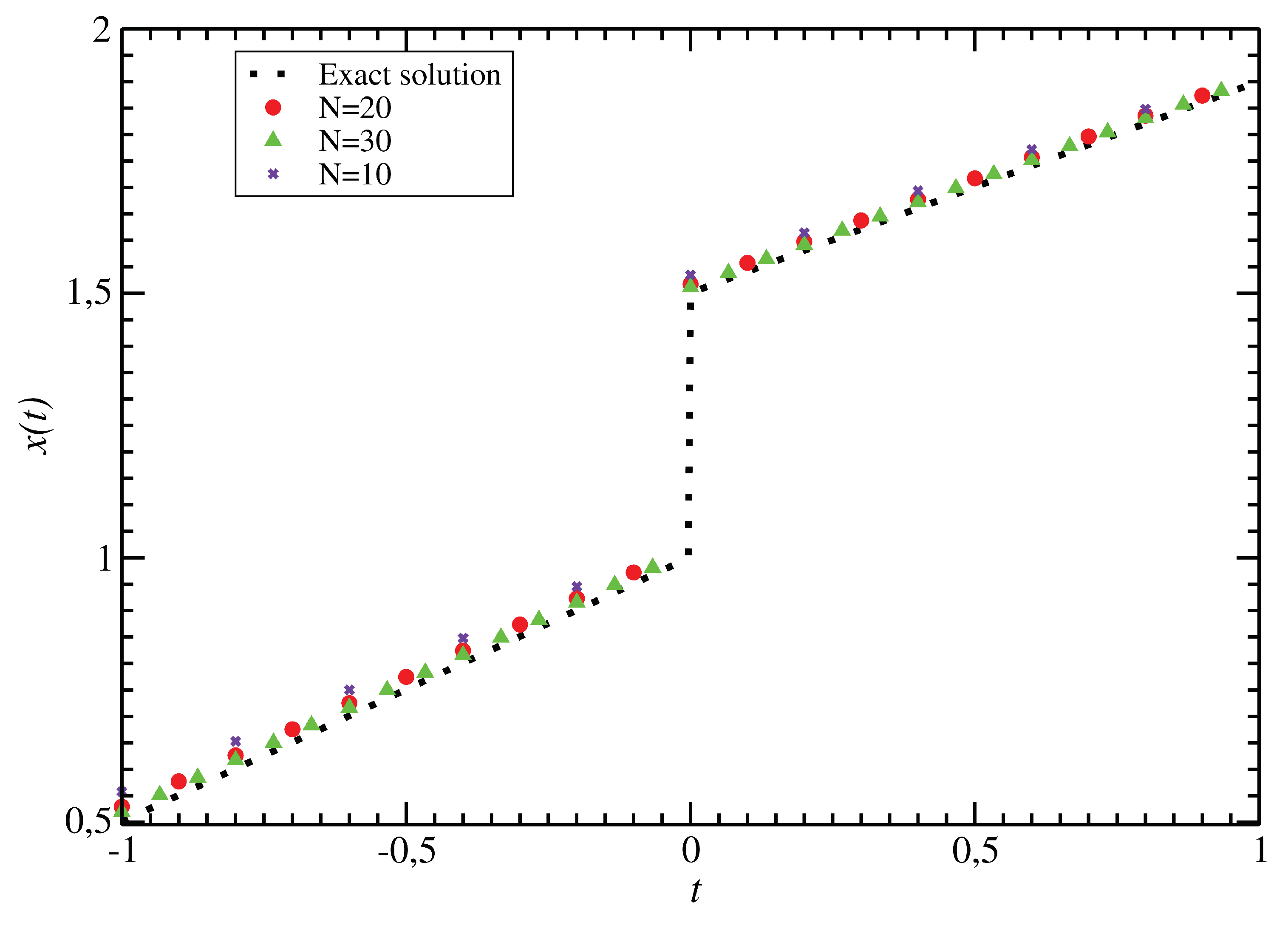
In Section 3.1 the continuous method is applied to linear hypersingular integral equations with the singularities of the second order. The conditions for the unique solvability of the constructed computing scheme are obtained and the convergence of the sequence of approximate solutions to the exact one is proven. It is shown that for linear hypersingular integral equations, the method converges for sufficiently large N and for $b(t)\ne 0,t\in [-1,1]$.

(3)

In Section 3.2 the continuous method is applied to nonlinear hypersingular integral equations with the singularities of the second order. Conditions are given for the convergence of the constructed iterative spline-collocation method to the solution of a nonlinear hypersingular integral equation. It should be noted that the method is applicable to hypersingular integral equations of the first and second kinds.

The detailed bibliography of approximation methods of hypersingular integral equations of the first and the second kinds is given in [32]. The bibliography on solving hypersingular integral equations of the first kind is presented in [45].

Mostly, papers devoted to hypersingular integral equations of the first kind focused to seek solutions in the class of functions $\sqrt{1-t^2}\varphi (t)$, where $\varphi (t)$ is a smooth function. The presented method provides solutions in a general form.

The theoretical justification of the method is based on Lyapunov stability theory. It connects convergence of the method to the sign of the approximate system matrix logarithmic norm.

Said justification has advantages that allow us

1.

To obtain a set of convergence conditions owing to logarithmic norm values in various spaces;

2.

To determine the norm of the inverse matrix of an approximate system;

3.

To determine stability boundaries for solutions with respect to variations of kernels and right-hand sides of the equations.

The major advantage of the method for nonlinear equations is as follows.

The Newton–Kantorovich method requires the Frechet derivative reversibility at each iteration step. Similar conditions are required when using other iteration methods. Our method lacks such a deficiency. It does not put any restrictions on the Frechet derivative of the nonlinear operator.

References

1. Bogolubov, N.N.; Mesheryakov, V.A.; Tavkhelidze, A.N. An application of Muskhelishvili’s methods in the theory of elementary particles. In Proceedings of the Symposium on Solid Mechanics and Related Problems of Analysis, Metsniereba, Tbilisi; 1971; Volume 1, pp. 5–11. (In Russian). [Google Scholar]
2. Brown, D.D.; Jackson, A.D. The Nucleon-Nucleon Interaction; North-Holland: Amsterdam, The Netherlands, 1976. [Google Scholar]
3. Faddeev, L.; Takhtajan, L. Hamiltonian Approach to Solution Theory; Springer: Berlin, Germany, 1986. [Google Scholar]
4. Ioakimidis, N.I. Two methods for the numerical solution of Bueckher’s singular integral equation for plane elasticity crack problems, Comput. Methods Appl. Mech. Engrg. 1982, 2, 169–177. [Google Scholar] [CrossRef]
5. Lifanov, I.K.; Poltavskii, L.N.; Vainikko, G.M. Hypersingular Integral Equations and their Applications; Chapman Hall/CRC: Boca Raton, FL, USA; CRC Press Company: London, UK; New York, NY, USA; Washington, DC, USA, 2004. [Google Scholar]
6. Mandal, B.N.; Chakrabarti, A. Applied Singular Integral Equations; CRC Press: Boca Raton, FL, USA, 2011; 260p. [Google Scholar]
7. Boykov, I.V.; Boykova, A.I. Analytical methods for solution of hypersingular and polyhypersingular integral equations. arXiv 2019, arXiv:1901.04880v1. [Google Scholar]
8. Gakhov, F.D. Boundary Value Problems; Dover Publication: Mineola, NY, USA, 1990; 561p. [Google Scholar]
9. Ivanov, V.V. The Theory of Approximate Methods and their Application to the Numerical Solution of Singular Integral Equations; Noordhoff International Publishing: Leiden, The Netherlands, 1976. [Google Scholar]
10. Gohberg, I.C.; Fel’dman, I.A. Convolution Equation and Projection Methods for Their Solution; Nauka: Moscow, Russia, 1971; English Translation: Translations of Mathematical Monographss Volume 41; American Mathematical Society: Providence, RI, USA, 1974. [Google Scholar]
11. Golberg, M.A. Introduction to the numerical solution of Cauchy singular integral equations. In Mathematical Concepts and Methods in Science and Engineering; Plenum Press: New York, NY, USA, 1990; Volume 42. [Google Scholar]
12. Michlin, S.G.; Prossdorf, S. Singular Integral Operatoren; Acad.-Verl.: Berlin, Germany, 1980. [Google Scholar]
13. Boykov, I.V. Approximate Methods of Solution of Singular Integral Equations; The Penza State University: Penza, Russia, 2004. (In Russian) [Google Scholar]
14. Boykov, I.V. Numerical methods for solutions of singular integral equations. arXiv 1973, arXiv:1610.09611. [Google Scholar]
15. Capobiano, M.R.; Criscuolo, G.; Junghanns, P. On the numerical solution of a nonlinear integral equation of Prandtl’s type. In Operator Theory: Advances and Applications; Birkhauser Verlag: Basel, Switzerland, 2005; Volume 160, pp. 53–79. [Google Scholar]
16. Oseledets, I.V.; Tyrtyshnicov, E.E. Approximate invention of matrices in the process of solving hypersingular integral equation. Comput. Math. Math. Phys. 2005, 45, 302–313. [Google Scholar]
17. Golberg, M.A. The convergence of several algorithms for solving integral equations with finite-part integrals, I. Integral Equ. 1983, 5, 329–340. [Google Scholar] [CrossRef]
18. Golberg, M.A. The convergence of several algorithms for solving integral equations with finite-part integrals, II. Integral Equ. 1985, 9, 267–275. [Google Scholar] [CrossRef]
19. Lifanov, I.K. Singular Integral Equations and Discrete Vortices; VSP: Utrecht, The Netherlands, 1996. [Google Scholar]
20. Boykov, I.V.; Zakharova Yu, F. An approximate solution to hypersingular integro-differential equations. Univ. Proc. Volga Reg. Phys. Math. Sci. Math. 2010, 1, 80–90. (In Russian) [Google Scholar]
21. Boykov, I.V.; Boykova, A.I. An approximate solution of hypersingular integral equations with odd singularities of integer order. Univ. Proc. Volga Reg. Phys. Math. Sci. Math. 2010, 3, 15–27. (In Russian) [Google Scholar]
22. Boykov, I.V.; Ventsel, E.S.; Boykova, A.I. An approximate solution of hypersingular integral equations. Appl. Numer. Math. 2010, 60, 607–628. [Google Scholar] [CrossRef]
23. Boykov, I.V.; Ventsel, E.S.; Roudnev, V.A.; Boykova, A.I. An approximate solution of nonlinear hypersingular integral equations. Appl. Numer. Math. 2014, 86, 1–21. [Google Scholar] [CrossRef]
24. Boykov, I.V.; Roudnev, V.A.; Boykova, A.I.; Baulina, O.A. New iterative method for solving linear and nonlinear hypersingular integral equations. Appl. Numer. Math. 2018, 127, 280–305. [Google Scholar] [CrossRef]
25. Kaya, A.C.; Erdogan, F. On The Solution of Integral Equations with Strongly Singular Kernels. Quart. Appl. Math. 1987, 95, 105–122. [Google Scholar] [CrossRef] [Green Version]
26. Eshkuvatov, Z.K.; Zulkarnain, F.S.; Nik Long, N.M.A.; Muminov, Z. Modified homotopy perturbation method for solving hypersingular integral equations of the first kind. SpringerPlus 2016, 5, 1473. [Google Scholar] [CrossRef] [Green Version]
27. Boykov, I.V.; Boykova, A.I.; Syomov, M.A. An approximate solution of hypersingular integral equations of the first kind. Univ. Proc. Volga Reg. Phys. Math. Sci. Math. 2015, 3, 11–27. (In Russian) [Google Scholar]
28. Boykov, I.V.; Boykova, A.I. Approximate methods for solving hypersingular integral equations of the first kind with second-order singularities on classes of functions with weights (1-t2)-1/2. Univ. Proc. Volga Reg. Phys. Math. Sci. Math. 2017, 2, 79–90. (In Russian) [Google Scholar]
29. Boykov, I.V.; Boykova, A.I. An approximate solution of hypersingular integral equations of the first kind with singularities of the second order on the class of functions with weight ((1-t)/(1+t))±1/2. Univ. Proc. Volga Reg. Phys. Math. Sci. Math. 2019, 3, 76–92. (In Russian) [Google Scholar]
30. Lifanov, I.K.; Nenashev, A.S. Hypersingular integral equations and the theory of wire antennas. Diff. Equ. 2005, 41, 126–145. [Google Scholar] [CrossRef]
31. Lifanov, I.K.; Nenashev, A.S. Analysis of Some Computational Schemes for a Hypersingular Integral Equation on an Interval. Diff. Equ. 2005, 41, 1343–1348. [Google Scholar] [CrossRef]
32. Boykov, I.V. Analytical and numerical methods for solving hypersingular integral equations. Dyn. Syst. 2019, 9, 244–272. (In Russian) [Google Scholar]
33. Boikov, I.V. On a continuous method for solving nonlinear operator equations. Differ. Equ. 2012, 48, 1308–1314. [Google Scholar] [CrossRef]
34. Daletskii Yu, L.; Krein, M.G. Stability of Solutions of Differential Equations in Banach Space; Nauka: Moscow, Russia, 1970; 536p, English Translation: Translations of Mathematical Monographss, Volume 43; American Mathematical Society: Providence, RI, USA, 1974. (In Russian) [Google Scholar]
35. Lozinskii, S.M. Note on a paper by V.S. Godlevskii. Ussr Comput. Math. Math. Phys. 1973, 13, 232–234. [Google Scholar] [CrossRef]
36. Boikov, I.V. On the stability of solutions of differential and difference equations in critical cases. Soviet Math. Dokl. 1991, 42, 630–632. [Google Scholar]
37. Boikov, I.V. Stability of Solutions of Differential Equations; Publishing House of Penza State University: Penza, Russia, 2008; 24p. (In Russian) [Google Scholar]
38. Browder, F.E. Nonlinear mappings of the nonexpansive and accretive type in Banach spaces. Bull. Am. Math. Soc. 1967, 73, 875–882. [Google Scholar] [CrossRef] [Green Version]
39. Malkowski, E.; Rakoćević, V. Advanced Functional Analysis; CRS Press, Taylor and Francis Group: Boca Raton, FL, USA, 2019. [Google Scholar]
40. Ćirić, L.; Rafiq, A.; Radenović, S.; Rajović, M. Jeong Sheok Ume On Mann implicit iterations for strongly accreative and strongly pseudo-contractive mappings. Appl. Math. Comput. 2008, 198, 128–137. [Google Scholar]
41. Todoriević, V. Harmonic Quasiconformal Mappings and Hyperbolic Type Metrics; Springer Nature: Cham, Switzerland, 2019. [Google Scholar]
42. Todoriević, V. Subharmonic behavior and quasiconformal mappings. Anal. Math. Phys. 2019, 9, 1211–1225. [Google Scholar] [CrossRef]
43. Hadamard, J. Lectures on Cauchy’s Problem in Linear Partial Differential Equations; Dover Publ. Inc.: New York, NY, USA, 1952. [Google Scholar]
44. Chikin, L.A. Special cases of the Riemann boundary value problems and singular integral equations. Sci. Notes Kazan State Univ. 1953, 113, 53–105. (In Russian) [Google Scholar]
45. Chan, Y.-S.; Fannjiang, A.C.; Paulino, G.H. Integral equations with hypersingular kernels-theory and applications to fracture mechanics. Int. J. Eng. Sci. 2003, 41, 683–720. [Google Scholar] [CrossRef] [Green Version]
Figure 1. Numerical solutions for the linear hypersingular equation with a discontinuous right-hand side example.
Axioms 09 00074 g001
Figure 2. Numerical solution for the nonlinear hypersingular equation with a discontinuous right-hand side example.
Axioms 09 00074 g002