Global Solvability of a Fifth-Order KdV Equation Posed on Finite Interval [0, d]

Abstract

This paper establishes the global existence and uniqueness of solutions to the initial-boundary value problem for a fifth-order KdV equation posed on a finite interval [0, d]. Overcoming the challenge of global solvability imposed by non-conservative boundary conditions, we introduce a nonlinear boundary feedback mechanism inspired by control theory to enforce energy dissipation. The proof hinges on deriving rigorous a priori estimates that capture both the Kato smoothing effect and boundary trace regularity, complemented by a tailored nonlinear estimate to handle the feedback term. Consequently, local solutions are extended to global ones. Furthermore, comprehensive numerical experiments validate the proposed approach and yield strong empirical evidence of exponential energy decay, a property crucial for control applications.

1. Introduction

To describe the weakly nonlinear hydromagnetic waves in a cold collision-free plasma, Kakutani and Ono [1] and subsequently Hasimoto [2] proposed the following fifth-order dispersive equation

$$u_t+\alpha u_x+\beta u_{3x}+\gamma u_{5x}+{\left(u^2\right)}_x=0.$$

Since this equation closely resembles the classical KdV equation

$$u_t+\alpha u_x+\beta u_{3x}+{\left(u^2\right)}_x=0$$

from both physical and mathematical perspectives, it is commonly referred to as the fifth-order KdV equation.

Over the past two decades, as a typical dispersive equation, the fifth-order KdV equation has been extensively studied regarding both its initial value problem (IVP) and initial boundary value problem (IBVP). Herein, we review the literature closely related to this paper to help outline the research progress and explore future research directions.

Regarding the IVP, research has primarily focused on the existence of low-regularity solutions. For instance, in 2005, Cui and Tao [3] showed that the IVP for the fifth-order KdV equation is locally well-posed in $H^s$ for $s>\frac{1}{4}$. Subsequently, in 2007, Wang, Cui, and Deng [4] improved these results by demonstrating that this local well-posedness in $H^s$ holds for $s>-\frac{7}{5}$, and that the solution is globally well-posed for $s>-\frac{1}{2}$. Between 2010 and 2013, sharp local solvability was achieved, and significant progress was made in global solvability, as reported in [5,6,7,8].

As for the IBVP, a series of fruitful results have been established. In 2014, Zhao and Zhang [9] investigated the boundary smoothing properties and established the local solvability of the fifth-order KdV equation under specific boundary conditions: $u(0,t)=g_1\left(t\right),u(d,t)=g_2\left(t\right),u_x(0,t)=g_3\left(t\right),u_x(d,t)=g_4\left(t\right),u_{2x}(d,t)=g_5\left(t\right)$. Later, Zhao and Zhang [10] systematically demonstrated local solvability under general boundary conditions: $B_{1}u=g_1\left(t\right),B_{2}u=g_2\left(t\right),B_{3}u=g_3\left(t\right),B_{4}u=g_4\left(t\right),B_{5}u=g_5\left(t\right)$ (encompassing 16 admissible boundary value combinations from Case a to Case p). With the foundational issue of solvability well addressed, research naturally progressed toward the long-time dynamical behavior of the system, particularly boundary stabilization. Notably, in the context of boundary stabilization, Araruna et al. [11] first explored the exponential energy decay of the Kawahara equation on a bounded domain, identifying the critical interval length. Furthermore, accounting for the unavoidable time delays in practical engineering, Capistrano-Filho et al. [12] investigated the stability of the Kawahara equation with time-delayed boundary control, demonstrating that the energy decays exponentially under suitable delayed feedback.

Among the 16 admissible boundary value combinations mentioned in [10], energy conservation holds under four specific cases (Case a, Case c, Case i, and Case j). According to the recent study by Zhao, Wang, and Bao [13], the local solutions corresponding to these four conservative cases have been successfully extended to global ones. However, for the remaining twelve non-conservative boundary conditions, the lack of inherent dissipation makes achieving global existence an open and challenging problem. To overcome this, a natural strategy is to introduce a nonlinear boundary feedback mechanism to artificially induce the necessary dissipation. This approach is theoretically viable due to the recent progress by Zhao and Hou [14], who resolved the well-posedness of the fifth-order KdV equation with nonlinear boundary conditions. Building upon this foundation, we consider incorporating a specific nonlinear feedback into one of the non-conservative cases to extend the local solution to a global one. For example, under the nonlinear feedback $\frac{1}{3}{\left[u(d,t)\right]}^2$, the solution to the IBVP

$$\left\{\begin{array}{cc}{u}_t-u_{5x}={\left(u^2\right)}_x,\hfill & 0<x<d,t>0,\hfill \\ u(x,0)=\varphi \left(x\right),\hfill & 0<x<d,\hfill \\ u(0,t)=u_x(0,t)=u_{2x}(d,t)=0,\hfill & \\ u_{3x}(d,t)=0,u_{4x}(d,t)+\frac{1}{3}{\left[u(d,t)\right]}^2=0,\hfill & t>0,\hfill \end{array}\right.$$

(1)

satisfies

$$\begin{array}{ccc}\hfill \frac{d}{dt}{\int }_0^d{u}^{2}dx& =& 2{\int }_0^{d}u(u_{5x}+{\left(u^2\right)}_x)dx\hfill \\ & =& 2u{u}_{4x}{|}_0^d-2u_x{u}_{3x}{|}_0^d+{\left[u_{2x}\right]}^2{|}_0^d+\frac{2}{3}{u}^3{|}_0^d\hfill \\ & =& -{\left[u_{2x}(0,t)\right]}^2\hfill \\ & \le & 0,\hfill \end{array}$$

which implies the $L^2$-bounded

$${\parallel u\left(t\right)\parallel }_{L^2\left([0,d]\right)}\le {\parallel \varphi \parallel }_{L^2\left([0,d]\right)}.$$

(2)

The uniform boundedness of the energy (2) suggests the existence of a global solution and the possibility of exponential stability. This paper investigates this issue. To facilitate the presentation of the main results, we first introduce some unified notation. The initial data belongs to $H_0^s(0,d)$, and the boundary data belongs to

$${\mathcal{H}}^s(0,T)\equiv G_0^{\frac{s+2}{5}}(0,T)\times G_0^{\frac{s+1}{5}}(0,T)\times G_0^{\frac{s}{5}}(0,T)\times G_0^{\frac{s-1}{5}}(0,T)\times G_0^{\frac{s-2}{5}}(0,T).$$

Thus, the overall data space is defined as

$$X_T^s\equiv H_0^s(0,d)\times {\mathcal{H}}^s(0,T).$$

Because the fifth-order KdV equation exhibits the Kato smoothing effect, the solution space must reflect this particular property. Therefore, the base function space is initially chosen as

$$Y_T^s\equiv C([0,T];H^s(0,d))\cap L^2([0,T_f];H^{s+2}(0,d)).$$

However, due to the nonlinear boundary feedback, boundary trace regularity is also essential. Consequently, the solution space is ultimately defined as

$${\mathcal{Y}}_T^s\equiv \{u\in Y_T^s:{\displaystyle \sum _{k=0}^4}{\parallel u\parallel }_{L^{\infty }([0,d];H^{\frac{s+2-k}{5}}({\mathbb{R}}^{+}))}<\infty \}.$$

Now, let us introduce the main results of this paper:

Theorem 1.

For any $T>0$ and $s\in [0,5]$ with $s\ne \frac{j}{2}$ ($j=1,3,5,7,9$), and for any $\varphi \in H^s(0,d)$, the IBVP

$$\left\{\begin{array}{cc}{u}_t-u_{5x}={\left(u^2\right)}_x,\hfill & 0<x<d,t>0,\hfill \\ u(x,0)=\varphi \left(x\right),\hfill & 0<x<d,\hfill \\ u(0,t)=u_x(0,t)=u_{2x}(d,t)=0,\hfill & \\ u_{3x}(d,t)=0,u_{4x}(d,t)-\frac{1}{3}{\left[u(d,t)\right]}^2=0,\hfill & t>0\hfill \end{array}\right.$$

admits a unique solution $u\in {\mathcal{Y}}_T^s$.

The remainder of this paper is organized as follows:

• Section 2 provides the preliminaries, including essential estimates such as the smoothing effect, boundary trace regularity, and estimates for the quadratic nonlinearity.
• Section 3 is devoted to the proof of global solvability. The proof is divided into three steps: we first verify the special cases where $s=0$ and $s=5$ separately, and subsequently prove the case $0<s<5$ using nonlinear interpolation.
• Section 4 presents numerical experiments to validate the effectiveness of the proposed nonlinear boundary feedback mechanism and to visualize the exponential decay of the energy.
• Section 5 concludes the paper with several remarks and numerical simulations. Specifically, it provides numerical evidence to verify the exponential decay of the energy, discusses the technical bottlenecks regarding half-integer regularities, and outlines promising directions for future research, including rigorous decay proofs, engineering approximations, and extensions to more general IBVPs.

2. Preliminaries

Technically, the proof of well-posedness relies on deriving linear estimates (including the Kato smoothing and boundary trace estimates) and nonlinear estimates, followed by an application of the Banach fixed-point theorem. Thus, this preliminary section covers two components: the smoothing effect estimates, available in [10] and invoked directly, and the nonlinear estimates, which remain unaddressed and require a complete proof herein.

2.1. Smoothing Effect and Trace Regularity

Following the standard procedure, by applying the superposition principle, we first decompose

$$\left\{\begin{array}{cc}{u}_t-u_{5x}=f,\hfill & \hfill 0<x<d,t>0,\\ u(x,0)=\varphi \left(x\right),\hfill & \hfill 0<x<d,\\ u(0,t)=g_1\left(t\right),u_x(0,t)=g_2\left(t\right),u_{2x}(d,t)=g_3\left(t\right),\hfill & \hfill t>0,\\ u_{3x}(d,t)=g_4\left(t\right),u_{4x}(d,t)=g_5\left(t\right),\hfill & \hfill t>0\end{array}\right.$$

(3)

into

$$\left\{\begin{array}{cc}{u}_t-u_{5x}=0,\hfill & \hfill 0<x<d,t>0,\\ u(x,0)=0,\hfill & \hfill 0<x<d,\\ u(0,t)=g_1\left(t\right),u_x(0,t)=g_2\left(t\right),u_{2x}(d,t)=g_3\left(t\right),\hfill & \hfill t>0,\\ u_{3x}(d,t)=g_4\left(t\right),u_{4x}(d,t)=g_5\left(t\right),\hfill & \hfill t>0\end{array}\right.$$

(4)

and

$$\left\{\begin{array}{cc}{u}_t-u_{5x}=f(x,t),\hfill & \hfill 0<x<d,t>0,\\ u(x,0)=\varphi \left(x\right),\hfill & \hfill 0<x<d,\\ u(0,t)=u_x(0,t)=u_{2x}(d,t)=0,\hfill & \hfill t>0,\\ u_{3x}(d,t)=u_{4x}(d,t)=0,\hfill & \hfill t>0.\end{array}\right.$$

(5)

By employing the multiplier technique and Laplace transform, the solution to (4) satisfies both the smoothing effect estimate

$${\parallel u\parallel }_{L^2({\mathbb{R}}^{+};H^{2+s}(0,d))}\le C{\parallel \overrightarrow{h}\parallel }_{H^s\left({\mathbb{R}}^{+}\right)}$$

and the trace regularity estimate

$${\parallel u\parallel }_{C(0,T];H^s(0,d))}+{\displaystyle \sum _{k=0}^4}{\parallel u\parallel }_{L^{\infty }([0,d];H^{\frac{s+2-k}{5}}({\mathbb{R}}^{+}))}\le C{\parallel \overrightarrow{h}\parallel }_{H^s\left({\mathbb{R}}^{+}\right)}.$$

Through an extensive strategy, the solution to (5) satisfies the following combined smoothing effect and trace regularity estimate:

$${\parallel u\parallel }_{C([0,T];H^s(0,d))}+{\parallel u\parallel }_{L^2(0,T;H^{2+s}(0,d))}+{\displaystyle \sum _{k=0}^4}{\parallel u\parallel }_{L^{\infty }([0,d];H^{\frac{s+2-k}{5}}({\mathbb{R}}^{+}))}\le C\left({\parallel \varphi \parallel }_{H^s(0,d)}+{\parallel f\parallel }_{L^1(0,T;H^s(0,d))}\right).$$

Finally, combining the estimates for (4) and (5) yields the following comprehensive result:

Lemma 1.

Let $T>0$ and $s\in [0,5]$. For any compatible $\varphi \in H^s(0,d)$ and $\overrightarrow{h}\in {\mathcal{H}}^s\left({\mathbb{R}}^{+}\right)$ and $f\in L^1(0,T_f;H^s(0,d))$, the IBV Problem (3) has a solution $u\in C([0,T];H^s(0,d))\cap L^2(0,T;H^{2+s}(0,d))$ satisfying

$${\parallel u\parallel }_{C([0,T];H^s(0,d))}+{\parallel u\parallel }_{L^2(0,T;H^{2+s}(0,d))}+{\displaystyle \sum _{k=0}^4}{\parallel u\parallel }_{L^{\infty }([0,d];H^{\frac{s+2-k}{5}}({\mathbb{R}}^{+}))}\le C\left({\parallel \varphi \parallel }_{H^s(0,d)}+\parallel \overrightarrow{h}{\parallel }_{{\mathcal{H}}^s\left({\mathbb{R}}^{+}\right)}+{\parallel f\parallel }_{L^1(0,T;H^s(0,d))}\right).$$

Proof. 

See [10] for the details. □

2.2. Nonlinear Estimates

We begin with the quadratic nonlinear source term ${\left(u^2\right)}_x$ appearing in the equation:

Lemma 2.

For any $s\ge 0$, there exists a constant $C>0$ such that for all $T>0$ and $u,v\in Y_T^s$,

$${\int }_0^T\parallel u{v}_x{\parallel }_{H^s(0,d)}d\tau \le C(T^{\frac{1}{2}}+T^{\frac{1}{4}}){\parallel u\parallel }_{Y_T^s}{\parallel v\parallel }_{Y_T^s}.$$

Proof. 

See [15]. □

Next, we address the quadratic nonlinear terms induced by the boundary feedback, such as $u{(0,t)}^2$ or $u{(d,t)}^2$:

Lemma 3.

For any $s\in [0,5]$, we have

$${\parallel uv\parallel }_{H^{\frac{s-2}{5}}(0,T)}\le C{T}^{\frac{7}{10}(1-\frac{s}{5})}{\parallel u\parallel }_{H^{\frac{s+2}{5}}(0,T)}{\parallel v\parallel }_{H^{\frac{s+2}{5}}(0,T)}.$$

Proof. 

For the case $s=0$, by utilizing the embedding $H^{-\frac{2}{5}}\hookleftarrow L^{\frac{10}{9}}$ and $H^{\frac{2}{5}}\hookrightarrow L^{10}$, along with Hölder’s inequality, we obtain

$$\begin{array}{cc}\hfill {\parallel uv\parallel }_{H^{-\frac{2}{5}}(0,T)}& \le {\parallel uv\parallel }_{L^{\frac{10}{9}}(0,T)}\hfill \\ \hfill & \le T^{\frac{7}{10}}{\parallel u\parallel }_{L^{10}(0,T)}{\parallel v\parallel }_{L^{10}(0,T)}\le T^{\frac{7}{10}}{\parallel u\parallel }_{H^{\frac{2}{5}}(0,T)}{\parallel v\parallel }_{H^{\frac{2}{5}}(0,T)}.\hfill \end{array}$$

For the case $s=5$, since $H^{\frac{3}{5}}(0,T)$ is a Banach algebra, it follows that

$${\parallel uv\parallel }_{H^{\frac{3}{5}}(0,T)}\le {\parallel u\parallel }_{H^{\frac{3}{5}}(0,T)}{\parallel v\parallel }_{H^{\frac{3}{5}}(0,T)}\le {\parallel u\parallel }_{H^{\frac{7}{5}}(0,T)}{\parallel v\parallel }_{H^{\frac{7}{5}}(0,T)}.$$

Finally, for the general case, we employ interpolation theory. Letting $\theta =1-\frac{s}{5}$, we have the interpolation identities

$${[H^{-\frac{2}{5}}(0,T),H^{\frac{3}{5}}(0,T)]}_{\theta }=H^{\frac{s-2}{5}},{[H^{\frac{2}{5}}(0,T),H^{\frac{7}{5}}(0,T)]}_{\theta }=H^{\frac{s+2}{5}}.$$

Interpolating between the bounds for $s=0$ and $s=5$ yields the desired estimate:

$${\parallel uv\parallel }_{H^{\frac{s-2}{5}}(0,T)}\le C{T}^{\frac{7}{10}\left(1-\frac{s}{5}\right)}{\parallel u\parallel }_{H^{\frac{s+2}{5}}(0,T)}{\parallel v\parallel }_{H^{\frac{s+2}{5}}(0,T)}.$$

□

3. Proof of Theorem 1

The proof of global solvability is organized into three systematic steps. We first establish the results for the endpoint Sobolev indices $s=0$ and $s=5$ separately and then employ nonlinear interpolation to extend the results to the intermediate range $0<s<5$.

Step 1. The case of $s=0$.

Theorem 2.

For any given $T_f>0$, the IBV problem

$$\left\{\begin{array}{cc}{u}_t-u_{5x}={\left(u^2\right)}_x,\hfill & \hfill 0<x<d,t>0,\\ u(x,0)=\varphi \left(x\right),\hfill & \hfill 0<x<d,\\ u(0,t)=u_x(0,t)=u_{2x}(d,t)=0,\hfill & \\ u_{3x}(d,t)=0,u_{4x}(d,t)=\frac{1}{3}{\left[u(d,t)\right]}^2,\hfill & \hfill t>0\end{array}\right.$$

(6)

has a unique solution $u\in {\mathcal{Y}}_T^0$ satisfying

$${\parallel u\parallel }_{{\mathcal{Y}}_T^0}\le {\alpha }_{0,T}{(\parallel \varphi \parallel }_{L^2(0,d)}{)\parallel \varphi \parallel }_{L^2(0,d)},$$

where ${\alpha }_{0,T}:{\mathbb{R}}^{+}\to {\mathbb{R}}^{+}$ is a nondecreasing, continuous function depending solely on T.

Proof. 

Let $0<\tau \le max\{1,T_f\}$ and $r>0$ be constants. Define a closed ball in ${\mathcal{Y}}_{\tau }^0$ by

$${\mathcal{B}}_{\tau ,r}=\left\{v\in {\mathcal{Y}}_{\tau }^0:{\parallel v\parallel }_{{\mathcal{Y}}_{\tau }^0}\le r\right\}.$$

Obviously, ${\mathcal{B}}_{\tau ,r}$ is a closed, bounded, and convex subset of ${\mathcal{Y}}_{\tau }^0$. We define a mapping $\mathsf{\Gamma }:{\mathcal{B}}_{\tau ,r}\to {\mathcal{Y}}_{\tau }^0$ by $u=\mathsf{\Gamma }\left(v\right)$, where u is the unique solution to the linearized IBV problem

$$\left\{\begin{array}{cc}{u}_t-u_{5x}=v{\partial }_{x}v,\hfill & \hfill 0<x<d,t>0,\\ u(x,0)=\varphi \left(x\right),\hfill & \hfill 0<x<d,\\ u(0,t)=u_x(0,t)=u_{2x}(d,t)=0,\hfill & \hfill t>0,\\ u_{3x}(d,t)=0,u_{4x}(d,t)=\frac{1}{3}{\left[v(d,t)\right]}^2,\hfill & \hfill t>0,\end{array}\right.$$

for a given $v\in {\mathcal{B}}_{\tau ,r}$.

Applying Lemmas 1–3, we obtain

$$\begin{array}{ccc}\hfill \parallel \mathsf{\Gamma }\left(v\right){\parallel }_{{\mathcal{Y}}_{\tau }^0}& \le & C_1{\parallel \varphi \parallel }_{L^2(0,d)}+C_2\parallel {\left[v(d,t)\right]}^2{\parallel }_{H^{-\frac{2}{5}}(0,\tau )}+C_3{\parallel v{v}_x\parallel }_{L^1(0,\tau ;L^2(0,d))}\hfill \\ & \le & C_1{\parallel \varphi \parallel }_{L^2(0,d)}+C_2{\tau }^{\frac{7}{10}}{\parallel v(d,t)\parallel }_{H^{\frac{2}{5}}(0,\tau )}^2+C_3({\tau }^{\frac{1}{2}}+{\tau }^{\frac{1}{4}}){\parallel v\parallel }_{{\mathcal{Y}}_{\tau }^0}^2\hfill \\ & <& C_1{\parallel \varphi \parallel }_{L^2(0,d)}+[C_2{\tau }^{\frac{7}{10}}+C_3({\tau }^{\frac{1}{2}}+{\tau }^{\frac{1}{4}})]{\parallel v\parallel }_{{\mathcal{Y}}_{\tau }^0}^2.\hfill \end{array}$$

Now, take $r=2C_1{\parallel \varphi \parallel }_{L^2(0,d)}$ and choose $0<\tau \le 1$ sufficiently small to ensure that $[C_2{\tau }^{\frac{7}{10}}+C_3({\tau }^{\frac{1}{2}}+{\tau }^{\frac{1}{4}})]r\le \frac{1}{3}$. Thus, for any $v\in {\mathcal{B}}_{\tau ,r}$, we have

$$\begin{array}{ccc}\hfill \parallel \mathsf{\Gamma }\left(v\right){\parallel }_{{\mathcal{Y}}_{\tau }^0}& \le & \frac{r}{2}+[C_2{\tau }^{\frac{7}{10}}+C_3({\tau }^{\frac{1}{2}}+{\tau }^{\frac{1}{4}})]r^2\hfill \\ & <& \frac{r}{2}+\frac{r}{3}=\frac{5}{6}r.\hfill \end{array}$$

This verifies that $\mathsf{\Gamma }$ maps ${\mathcal{B}}_{\tau ,r}$ into itself.

Next, for any $u,v\in {\mathcal{B}}_{\tau ,r}$, let $U\equiv \mathsf{\Gamma }\left(u\right)-\mathsf{\Gamma }\left(v\right)$. Then, U satisfies

$$\left\{\begin{array}{cc}{U}_t-U_{5x}={\left(u^2\right)}_x-{\left(v^2\right)}_x,\hfill & \hfill 0<x<d,t>0,\\ U(x,0)=0,\hfill & \hfill 0<x<d,\\ U(0,t)=U_x(0,t)=U_{2x}(d,t)=0,U_{3x}(d,t)=0,\hfill & \\ U_{4x}(d,t)=\frac{1}{3}\left[u(d,t)+v(d,t)\right]U(d,t),\hfill & \hfill t>0.\end{array}\right.$$

Applying Lemmas 1–3 again yields

$$\begin{array}{ccc}\hfill \parallel \mathsf{\Gamma }\left(u\right)-\mathsf{\Gamma }\left(v\right){\parallel }_{{\mathcal{Y}}_{\tau }^0}& \le & C_1\parallel \left[u(d,t)+v(d,t)\right]{U(d,t)\parallel }_{H^{-\frac{2}{5}}(0,\tau )}+C_2{\parallel {\left(u^2\right)}_x-{\left(v^2\right)}_x\parallel }_{L^1([0,\tau ];L^2(0,d))}\hfill \\ & \le & C_1{\tau }^{\frac{7}{10}}[{\parallel v\parallel }_{H^{\frac{2}{5}}(0,\tau )}+{\parallel u\parallel }_{H^{\frac{2}{5}}(0,\tau )}]{\parallel U\parallel }_{H^{\frac{2}{5}}(0,\tau )}\hfill \\ & & +C_2({\tau }^{\frac{1}{2}}+{\tau }^{\frac{1}{4}})[{\parallel u\parallel }_{{\mathcal{Y}}_{\tau }^0}+{\parallel v\parallel }_{{\mathcal{Y}}_{\tau }^0}]{\parallel U\parallel }_{{\mathcal{Y}}_{\tau }^0}\hfill \\ & \le & 2[C_1{\tau }^{\frac{7}{10}}+C_2({\tau }^{\frac{1}{2}}+{\tau }^{\frac{1}{4}})]r{\parallel U\parallel }_{{\mathcal{Y}}_{\tau }^0}\hfill \\ & <& \frac{2}{3}{\parallel u-v\parallel }_{{\mathcal{Y}}_{\tau }^0},\hfill \end{array}$$

which implies that $\mathsf{\Gamma }$ is a strict contraction on ${\mathcal{B}}_{\tau ,r}$.

By Banach’s fixed-point theorem, the mapping $\mathsf{\Gamma }$ admits a unique fixed point in ${\mathcal{B}}_{\tau ,r}$.

Owing to the a priori $L^2$-boundedness of the solution established in (2), we can iteratively extend the local existence time $\tau$ to any prescribed final time $T_f$. □

Step 2. The case of $s=5$.

Next, we prove that the IBV problem (6) is globally solvable in $H^5(0,d)$. Define the compatible initial data set as

$$D^5(0,d)=\left\{\varphi \in H^5(0,d):\varphi \left(0\right)={\varphi }^{\prime }\left(0\right)={\varphi }^{″}\left(d\right)={\varphi }^{\left(3\right)}\left(d\right)=0,{\varphi }^{\left(4\right)}\left(d\right)=\frac{1}{3}\varphi {\left(d\right)}^2\right\}.$$

Then, we have the following theorem:

Theorem 3.

Let $T_f>0$. For any $\varphi \in D^5(0,d)$, the IBV problem (6) has a unique solution $u\in {\mathcal{Y}}_T^5$ satisfying

$${\parallel u\parallel }_{{\mathcal{Y}}_T^5}\le {\alpha }_{5,T}{(\parallel \varphi \parallel }_{H^5(0,d)}{)\parallel \varphi \parallel }_{H^5(0,d)},$$

where ${\alpha }_{5,T}:{\mathbb{R}}^{+}\to {\mathbb{R}}^{+}$ is a nondecreasing continuous function depending solely on T.

Before proceeding to the proof, we first establish a priori estimates for a linear system with variable coefficients $g\left(t\right)$ and $h(x,t)$:

$$\left\{\begin{array}{cc}{u}_t-u_{5x}={\left(hu\right)}_x,\hfill & \hfill 0<x<d,t>0,\\ u(x,0)=\varphi \left(x\right),\hfill & \hfill 0<x<d,\\ u(0,t)=u_x(0,t)=u_{2x}(d,t)=0,\hfill & \\ u_{3x}(d,t)=0,u_{4x}(d,t)=g\left(t\right)u(d,t),\hfill & \hfill t>0.\end{array}\right.$$

(7)

Proposition 1.

Let $T_f>0$ be given. Assume that $g\in H^{\frac{2}{5}}(0,T_f)$ and $h\in {\mathcal{Y}}_T^0$. Then, for any $\varphi \in L^2(0,d)$, the IBV problem (7) has a unique solution $u\in {\mathcal{Y}}_T^0$ satisfying

$${\parallel u\parallel }_{{\mathcal{Y}}_T^0}\le \mu ({\parallel h\parallel }_{{\mathcal{Y}}_T^0}+{\parallel g\parallel }_{H^{\frac{2}{5}}(0,T)}){\parallel \varphi \parallel }_{L^2(0,d)},$$

where $\mu :{\mathbb{R}}^{+}\to {\mathbb{R}}^{+}$ is a $T_f$-dependent continuous nondecreasing function independent of ϕ.

Proof. 

Let $0<\tau \le max\{1,T\}$ and $r>0$ be constants. Define the closed ball

$${\mathcal{B}}_{\tau ,r}=\left\{v\in {\mathcal{Y}}_{\tau }^0:{\parallel v\parallel }_{{\mathcal{Y}}_{\tau }^0}\le r\right\},$$

which is a bounded, closed, and convex subset of ${\mathcal{Y}}_{\tau }^0$. Define the mapping $\mathsf{\Gamma }:{\mathcal{B}}_{\tau ,r}\to {\mathcal{Y}}_{\tau }^0$ by $u=\mathsf{\Gamma }\left(v\right)$, where u is the solution to (7).

Applying Lemmas 1–3, we have

$$\begin{array}{ccc}\hfill \parallel \mathsf{\Gamma }\left(v\right){\parallel }_{{\mathcal{Y}}_{\tau }^0}& \le & C_1{\parallel \varphi \parallel }_{L^2(0,d)}+C_2{\parallel g\left(t\right)v(d,t)\parallel }_{H^{-\frac{2}{5}}(0,\tau )}+C_3{\parallel {\partial }_x\left(hv\right)\parallel }_{L^1(0,\tau ;L^2(0,d))}\hfill \\ & \le & C_1{\parallel \varphi \parallel }_{L^2(0,d)}+C_2{\tau }^{\frac{7}{10}}{\parallel g\parallel }_{H^{\frac{2}{5}}(0,\tau )}{\parallel v(d,t)\parallel }_{H^{\frac{2}{5}}(0,\tau )}+C_3({\tau }^{\frac{1}{2}}+{\tau }^{\frac{1}{4}}){\parallel h\parallel }_{{\mathcal{Y}}_{\tau }^0}{\parallel v\parallel }_{{\mathcal{Y}}_{\tau }^0}\hfill \\ & \le & C_1{\parallel \varphi \parallel }_{L^2(0,d)}+[C_2{\tau }^{\frac{7}{10}}{\parallel g\parallel }_{H^{\frac{2}{5}}(0,\tau )}+C_3({\tau }^{\frac{1}{2}}+{\tau }^{\frac{1}{4}}){\parallel h\parallel }_{{\mathcal{Y}}_{\tau }^0}]{\parallel v\parallel }_{{\mathcal{Y}}_{\tau }^0}.\hfill \end{array}$$

Let $r=2C_1{\parallel \varphi \parallel }_{L^2(0,d)}$ and choose $0<\tau \le 1$ sufficiently small such that

$$[C_2{\tau }^{\frac{7}{10}}{\parallel g\parallel }_{H^{\frac{2}{5}}(0,\tau )}+C_3({\tau }^{\frac{1}{2}}+{\tau }^{\frac{1}{4}}){\parallel h\parallel }_{{\mathcal{Y}}_{\tau }^0}]\le \frac{1}{3}.$$

Then, for any $v\in {\mathcal{B}}_{\tau ,r}$, we obtain

$$\parallel \mathsf{\Gamma }\left(v\right){\parallel }_{{\mathcal{Y}}_{\tau }^0}<\frac{r}{2}+\frac{r}{3}=\frac{5}{6}r,$$

demonstrating that $\mathsf{\Gamma }$ maps ${\mathcal{B}}_{\tau ,r}$ into itself.

For any $u,v\in {\mathcal{B}}_{\tau ,r}$, let $U\equiv u-v$. Then, U satisfies

$$\left\{\begin{array}{cc}{U}_t-U_{5x}={\left[hU\right]}_x,\hfill & \hfill 0<x<d,t>0,\\ U(x,0)=0,\hfill & \hfill 0<x<d,\\ U(0,t)=U_x(0,t)=U_{2x}(d,t)=0,\hfill & \\ U_{3x}(d,t)=0,U_{4x}(d,t)=g\left(t\right)U(d,t),\hfill & \hfill t>0.\end{array}\right.$$

Using Lemmas 1–3 once more, we deduce

$$\begin{array}{ccc}\hfill \parallel \mathsf{\Gamma }\left(u\right)-\mathsf{\Gamma }\left(v\right){\parallel }_{{\mathcal{Y}}_{\tau }^0}& \le & C_1{\parallel g\left(t\right)U(d,t)\parallel }_{H^{-\frac{2}{5}}(0,\tau )}+C_2{\parallel h{\partial }_{x}U\parallel }_{L^1([0,\tau ];L^2(0,d))}\hfill \\ & \le & [C_1{\tau }^{\frac{7}{10}}{\parallel g\parallel }_{H^{\frac{2}{5}}(0,\tau )}+C_2({\tau }^{\frac{1}{2}}+{\tau }^{\frac{1}{4}}){\parallel h\parallel }_{{\mathcal{Y}}_{\tau }^0}]{\parallel U\parallel }_{{\mathcal{Y}}_{\tau }^0}\hfill \\ & <& \frac{1}{3}{\parallel u-v\parallel }_{{\mathcal{Y}}_{\tau }^0}.\hfill \end{array}$$

Thus, $\mathsf{\Gamma }$ is a contraction on ${\mathcal{B}}_{\tau ,r}$.

By the contraction mapping principle, $\mathsf{\Gamma }$ has a unique fixed point in ${\mathcal{B}}_{\tau ,r}$. It is important to note that the local existence time $\tau$ depends only on ${\parallel g\parallel }_{H^{\frac{2}{5}}(0,T)}+{\parallel h\parallel }_{{\mathcal{Y}}_T^0}$, and not directly on ${\parallel \varphi \parallel }_{L^2(0,d)}$. Using a standard continuous extension argument, we can extend the solution iteratively to obtain $\tau =T$. □

Proof of Theorem 1. 

For any $\varphi \in D^5(0,d)$, Theorem 2 guarantees a unique solution $u\in {\mathcal{Y}}_T^0$ to the IBV problem (6). Let $v=u_t$. Differentiating (6) with respect to t yields

$$\left\{\begin{array}{cc}{v}_t-v_{5x}=2{\left(uv\right)}_x,\hfill & \hfill 0<x<d,t>0,\\ v(x,0)={\varphi }^{*}\left(x\right),\hfill & \hfill 0<x<d,\\ v(0,t)=v_x(0,t)=v_{2x}(d,t)=0,\hfill & \\ v_{3x}(d,t)=-\frac{2}{3}u(d,t)v(d,t),\hfill & \hfill t>0,\end{array}\right.$$

(8)

where the initial data is computed as ${\varphi }^{*}\left(x\right)={\varphi }^{\left(5\right)}\left(x\right)+2\varphi \left(x\right){\varphi }^{\prime }\left(x\right)$. This is precisely in the form of (7) with $h=2u$ and $g\left(t\right)=-\frac{2}{3}u(d,t)$. □

By Proposition 1, it follows that $v=u_t\in {\mathcal{Y}}_T^0$. Since $u_{5x}=u_t+{\left(u^2\right)}_x$, the right-hand side belongs to ${\mathcal{Y}}_T^0$, which directly implies $u\in {\mathcal{Y}}_T^5$.

Step 3. The case of $0<s<5$.

Finally, we demonstrate that the IBV problem (6) is globally solvable in $H^s(0,d)$ for $s\in (0,5)$.

Theorem 4.

Let $T>0$, and $s\in (0,5)$ with $s\ne \frac{j}{2}$ for $j=1,3,5,7,9$. Then, for any $\varphi \in H^s(0,d)$, the IBV problem (6) has a unique solution $u\in {\mathcal{Y}}_T^s$ satisfying

$${\parallel u\parallel }_{{\mathcal{Y}}_T^s}\le {\alpha }_{s,T}{(\parallel \varphi \parallel }_{H^s(0,d)}{)\parallel \varphi \parallel }_{H^s(0,d)},$$

where ${\alpha }_{s,T}:{\mathbb{R}}^{+}\to {\mathbb{R}}^{+}$ is a nondecreasing and continuous function depending only on T.

Proof. 

Building upon Theorems 2 and 3, for any given $T>0$, the IBV problem (6) defines a nonlinear mapping $K:H^j(0,d)\to {\mathcal{Y}}_T^j$ for $j=0,5$. Furthermore, the following estimates hold:

• For any ${\varphi }_1,{\varphi }_2\in L^2(0,d)$,

  $$\parallel K\left({\varphi }_1\right)-K\left({\varphi }_2\right){\parallel }_{{\mathcal{Y}}_T^0}\le {\alpha }_{0,T}(max\{\parallel {\varphi }_1{\parallel }_{L^2},\parallel {\varphi }_2{\parallel }_{L^2}\left\}\right)\parallel {\varphi }_1-{\varphi }_2{\parallel }_{L^2(0,d)}.$$
• For any $\varphi \in H^5(0,d)$,

  $${\parallel K\left(\varphi \right)\parallel }_{{\mathcal{Y}}_T^5}\le {\alpha }_{5,T}{(\parallel \varphi \parallel }_{L^2(0,d)}{)\parallel \varphi \parallel }_{H^5(0,d)}.$$

According to Tartar’s nonlinear interpolation theory [16], the nonlinear map $K:H^s(0,d)\to {\mathcal{Y}}_T^s$ is well-defined for any $s\in (0,5)$, provided that $s\ne \frac{j}{2}$ for $j=1,3,5,7,9$. Moreover, the solution satisfies

$${\parallel K\left(\varphi \right)\parallel }_{{\mathcal{Y}}_T^s}\le {\alpha }_{s,T}{(\parallel \varphi \parallel }_{H^s(0,d)}{)\parallel \varphi \parallel }_{H^s(0,d)},\forall \varphi \in H^s(0,d),$$

with the interpolating function given by

$${\alpha }_{s,T}\left(r\right)={\alpha }_{0,T}^{1-\frac{s}{5}}\left(r\right){\alpha }_{5,T}^{\frac{s}{5}}\left(r\right).$$

For $\varphi \in H^s(0,d)$, $u=K\left(\varphi \right)\in {\mathcal{Y}}_T^s$ is the desired global solution to the IBV problem (6). □

4. Numerical Example

To bridge the gap between the abstract mathematical framework and practical dynamical behavior, we present numerical experiments in this section. Specifically, we simulate the initial-boundary value problem

$$\left\{\begin{array}{cc}{u}_t-u_{5x}={\left(u^2\right)}_x,\hfill & 0<x<2,t>0,\hfill \\ u(x,0)=-10x^2{(x-2)}^2,\hfill & 0<x<2,\hfill \\ u(0,t)=u_x(0,t)=u_{2x}(2,t)=0,\hfill & \\ u_{3x}(2,t)=0,u_{4x}(2,t)=\frac{1}{3}{\left[u(2,t)\right]}^2,\hfill & t>0\hfill \end{array}\right.$$

(9)

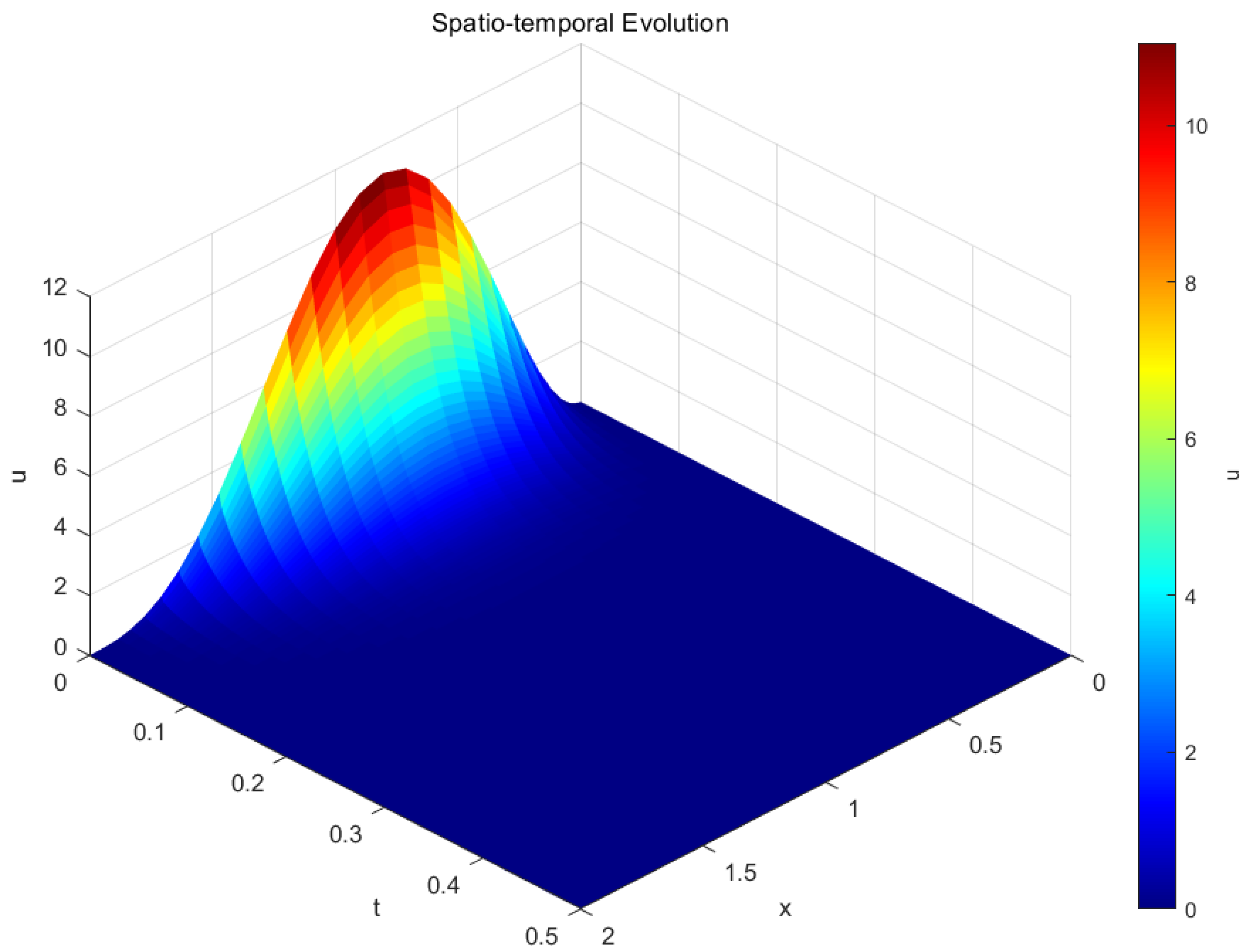
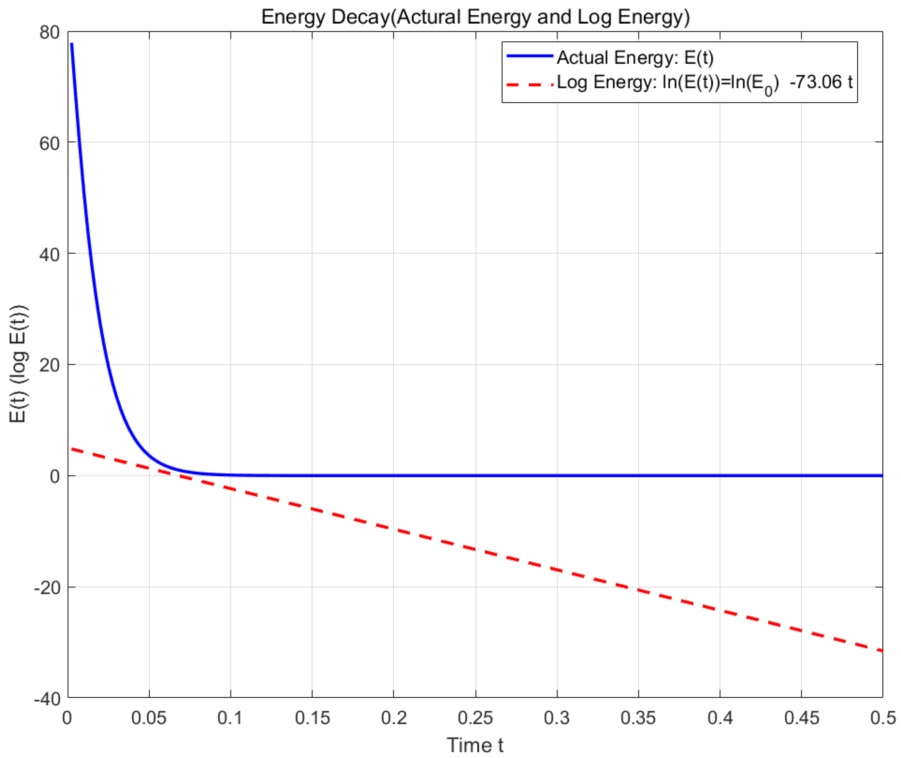
using a Chebyshev collocation method combined with a semi-implicit (linearized IMEX) time integrator. We discretize the spatial domain using $N=32$ Chebyshev collocation points and advance the solution with a time step $\Delta t={10}^{-5}$ see [17]. The numerical results are shown in Figure 1 and Figure 2.

Figure 1 illustrates the spatio-temporal evolution of the solution, revealing that the initial perturbation dissipates rapidly over time. Figure 2 displays the evolution of the energy $E\left(t\right)={\int }_0^d{u}^{2}dx$ on a semi-logarithmic scale. The energy trajectory exhibits a strictly linear profile, in exact accordance with the exponential decay law $E\left(t\right)\sim E_0{e}^{-\sigma t}$ for some $\sigma =73.06>0$.

This unambiguous exponential decay behavior strongly validates the effectiveness of the proposed boundary control mechanism and confirms that the system stabilizes rapidly, visually demonstrating the exponential stability of the system and validate the theoretical results established in the previous sections.

5. Concluding Remarks

Remark 1.

As mentioned in the introduction, the appropriate nonlinear boundary feedbacks can stabilize the nonlinear system. We have tailored nonlinear boundary feedback terms for the remaining 12 cases:

$$\begin{array}{cc}\hfill \mathit{Case}\mathbf{b}:& B_1^{\mathbf{b}}u\equiv u_x(d,t)=0,B_2^{\mathbf{b}}u\equiv u_x(0,t)=0,B_3^{\mathbf{b}}u\equiv u_{2x}(d,t)=0,\hfill \\ \hfill & B_4^{\mathbf{b}}u\equiv u_{4x}(d,t)-\frac{1}{3}{\left[u(d,t)\right]}^2=0,B_5^{\mathbf{b}}u\equiv u_{4x}(0,t)-\frac{1}{3}{\left[u(0,t)\right]}^2=0;\hfill \\ \hfill \mathit{Case}\mathbf{d}:& B_1^{\mathbf{d}}u\equiv u_{3x}(d,t)=0,B_2^{\mathbf{d}}u\equiv u_{3x}(0,t)=0,B_3^{\mathbf{d}}u\equiv u_{2x}(d,t)=0,\hfill \\ \hfill & B_4^{\mathbf{d}}u\equiv u_{4x}(d,t)-\frac{1}{3}{\left[u(d,t)\right]}^2=0,B_5^{\mathbf{d}}u\equiv u_{4x}(0,t)-\frac{1}{3}{\left[u(0,t)\right]}^2=0;\hfill \\ \hfill \mathit{Case}\mathbf{e}:& B_1^{\mathbf{e}}u\equiv u(0,t)=0,B_2^{\mathbf{e}}u\equiv u_x(d,t)=0,B_3^{\mathbf{e}}u\equiv u_x(0,t)=0,\hfill \\ \hfill & B_4^{\mathbf{e}}u\equiv u_{2x}(d,t)=0,B_5^{\mathbf{e}}u\equiv u_{4x}(d,t)-\frac{1}{3}{\left[u(d,t)\right]}^2=0;\hfill \\ \hfill \mathit{Case}\mathbf{f}:& B_1^{\mathbf{f}}u\equiv u(d,t)=0,B_2^{\mathbf{f}}u\equiv u_x(d,t)=0,B_3^{\mathbf{f}}u\equiv u_x(0,t)=0,\hfill \\ \hfill & B_4^{\mathbf{f}}u\equiv u_{2x}(d,t)=0,B_5^{\mathbf{f}}u\equiv u_{4x}(0,t)-\frac{1}{3}{\left[u(0,t)\right]}^2=0;\hfill \\ \hfill \mathit{Case}\mathbf{g}:& B_1^{\mathbf{g}}u\equiv u(0,t)=0,B_2^{\mathbf{g}}u\equiv u_{3x}(d,t)=0,B_3^{\mathbf{g}}u\equiv u_{3x}(0,t)=0,\hfill \\ \hfill & B_4^{\mathbf{g}}u\equiv u_{2x}(d,t)=0,B_5^{\mathbf{g}}u\equiv u_{4x}(d,t)-\frac{1}{3}{\left[u(d,t)\right]}^2=0;\hfill \\ \hfill \mathit{Case}\mathbf{h}:& B_1^{\mathbf{h}}u\equiv u(d,t)=0,B_2^{\mathbf{h}}u\equiv u_{2x}(d,t)=0,B_3^{\mathbf{h}}u\equiv u_{3x}(d,t)=0,\hfill \\ \hfill & B_4^{\mathbf{h}}u\equiv u_{3x}(0,t)=0,B_5^{\mathbf{h}}u\equiv u_{4x}(0,t)-\frac{1}{3}{\left[u(0,t)\right]}^2=0;\hfill \\ \hfill \mathit{Case}\mathbf{k}:& B_1^{\mathbf{k}}u\equiv u_x(0,t)=0,B_2^{\mathbf{k}}u\equiv u_{2x}(d,t)=0,B_3^{\mathbf{k}}u\equiv u_{3x}(d,t)=0,\hfill \\ \hfill & B_4^{\mathbf{k}}u\equiv u_{4x}(d,t)-\frac{1}{3}{\left[u(d,t)\right]}^2=0,B_5^{\mathbf{k}}u\equiv u_{4x}(0,t)-\frac{1}{3}{\left[u(0,t)\right]}^2=0;\hfill \\ \hfill \mathit{Case}\mathbf{l}:& B_1^{\mathbf{l}}u\equiv u_x(d,t)=0,B_2^{\mathbf{l}}u\equiv u_{2x}(d,t)=0,B_3^{\mathbf{l}}u\equiv u_{3x}(0,t)=0,\hfill \\ \hfill & B_4^{\mathbf{l}}u\equiv u_{4x}(d,t)-\frac{1}{3}{\left[u(d,t)\right]}^2=0,B_5^{\mathbf{l}}u\equiv u_{4x}(0,t)-\frac{1}{3}{\left[u(0,t)\right]}^2=0;\hfill \\ \hfill \mathit{Case}\mathbf{m}:& B_1^{\mathbf{m}}u\equiv u(0,t)=0,B_2^{\mathbf{m}}u\equiv u_x(0,t)=0,B_3^{\mathbf{m}}u\equiv u_{2x}(d,t)=0,\hfill \\ \hfill & B_4^{\mathbf{m}}u\equiv u_{3x}(d,t)=0,B_5^{\mathbf{m}}u\equiv u_{4x}(d,t)-\frac{1}{3}{\left[u(d,t)\right]}^2=0;\hfill \\ \hfill \mathit{Case}\mathbf{n}:& B_1^{\mathbf{n}}u\equiv u(d,t)=0,B_2^{\mathbf{n}}u\equiv u_x(0,t)=0,B_3^{\mathbf{n}}u\equiv u_{2x}(d,t)=0,\hfill \\ \hfill & B_4^{\mathbf{n}}u\equiv u_{3x}(0,t)=0,B_5^{\mathbf{n}}u\equiv u_{4x}(0,t)-\frac{1}{3}{\left[u(0,t)\right]}^2=0;\hfill \\ \hfill \mathit{Case}\mathbf{o}:& B_1^{\mathbf{o}}u\equiv u(d,t)=0,B_2^{\mathbf{o}}u\equiv u_x(0,t)=0,B_3^{\mathbf{o}}u\equiv u_{2x}(d,t)=0,\hfill \\ \hfill & B_4^{\mathbf{o}}u\equiv u_{3x}(d,t)=0,B_5^{\mathbf{o}}u\equiv u_{4x}(0,t)-\frac{1}{3}{\left[u(0,t)\right]}^2=0;\hfill \\ \hfill \mathit{Case}\mathbf{p}:& B_1^{\mathbf{p}}u\equiv u(d,t)=0,B_2^{\mathbf{p}}u\equiv u_x(d,t)=0,B_3^{\mathbf{p}}u\equiv u_{2x}(d,t)=0,\hfill \\ \hfill & B_4^{\mathbf{p}}u\equiv u_{3x}(0,t)=0,B_5^{\mathbf{p}}u\equiv u_{4x}(0,t)-\frac{1}{3}{\left[u(0,t)\right]}^2=0.\hfill \end{array}$$

Indeed, for

$$u_t-u_{5x}={\left(u^2\right)}_x,0<x<d,t>0,$$

(10)

we have

$$\frac{d}{dt}{\int }_0^d{u}^{2}dx=2{\int }_0^{d}u(u_{5x}+{\left(u^2\right)}_x)dx=2u{u}_{4x}{|}_0^d-2u_x{u}_{3x}{|}_0^d+{\left(u_{2x}\right)}^2{|}_0^d+\frac{2}{3}{u}^3{|}_0^d.$$

Thus, it is straightforward to see that energy decay occurs:

$$\frac{d}{dt}{\int }_0^d{u}^{2}dx\le 0.$$

Then, utilizing the analytical framework established in this paper, we conclude that global solvability holds under the above 12 boundary conditions:

Theorem 5.

Let $T>0$ and $s\in [0,5]$ with $s\ne \frac{j}{2}$ for $j=1,3,5,7,9$ be given. For any $\varphi \in H^s(0,d)$, the IBV problem

$$\left\{\begin{array}{cc}{u}_t-u_{5x}={\left(u^2\right)}_x,\hfill & \hfill 0<x<d,t>0,\\ u(x,0)=\varphi \left(x\right),\hfill & \hfill 0<x<d,\\ B_1^{\alpha }u=0,B_2^{\alpha }u=0,B_3^{\alpha }u=0,B_4^{\alpha }u=0,B_5^{\alpha }u=0,\alpha \in \{\mathbf{b},\mathbf{d},\dots ,\mathbf{p}\},\hfill & \hfill t>0\end{array}\right.$$

(11)

has a unique solution $u\in {\mathcal{Y}}_T^s$ satisfying

$${\parallel u\parallel }_{{\mathcal{Y}}_T^s}\le {\alpha }_{s,T}{(\parallel \varphi \parallel }_{H^s(0,d)}{)\parallel \varphi \parallel }_{H^s(0,d)},$$

where ${\alpha }_{s,T}:{\mathbb{R}}^{+}\to {\mathbb{R}}^{+}$ is a continuous nondecreasing function depending only on T.

Remark 2.

Although we have established the global well-posedness of the system and the energy dissipation naturally suggests exponential stability, a rigorous theoretical proof of this decay rate remains elusive due to current technical bottlenecks. Furthermore, the precise nonlinear boundary control established in our theoretical framework is primarily a mathematical construct; its exact implementation in real physical systems (e.g., plasma or shallow water waves) is far from straightforward from an engineering standpoint. To compensate for these theoretical and practical limitations, we resort to comprehensive numerical simulations in Section 5. These experiments serve as a practical alternative, providing strong empirical evidence that the energy indeed undergoes strict exponential decay—a property critical in control theory—thereby bridging the gap between our abstract mathematical framework and practical dynamical behavior.

Remark 3.

We note that the global solvability result excludes the half-integer indices $s\ne \frac{j}{2}$ ($j=1,3,5,7,9$). This restriction arises intrinsically from the derivation of the boundary smoothing effect and the trace regularity estimates. Specifically, at these critical half-integer regularities, the boundary traces fall into endpoint Sobolev spaces where the trace inequalities fail to hold, preventing the closure of the a priori estimates. It is important to emphasize that this is purely a mathematical technical bottleneck and bears no relation to the underlying physics of the system. Overcoming this technical barrier to establish well-posedness for the full spectrum of $s\in [0,5]$ remains a valuable direction for future research.

Remark 4.

Looking ahead, this work opens several promising avenues for future research. First, it would be of particular interest to rigorously establish the exponential decay rate of the energy under nonlinear boundary conditions, possibly through the use of Lyapunov functionals or observability inequalities. Second, a worthwhile direction is to explore whether the exact nonlinear boundary condition can be replaced by approximate or linearized alternatives, which would be significantly more amenable to engineering implementation. Finally, we envision that the proposed boundary feedback framework could be extended to dispersive systems or other high-order dispersive models subject to non-conservative boundary conditions.

References

1. Kakutani, T.; Ono, H. Weak non-linear hydromagnetic waves in a cold collision-free plasma. J. Phys. Soc. Jpn. 1969, 26, 1305–1318. [Google Scholar] [CrossRef] [Scilit]
2. Hasimoto, H. Water waves. Kagaku 1970, 40, 401–408. (In Japanese) [Google Scholar]
3. Cui, S.B.; Tao, S.P. Strichartz estimates for dispersive equations and solvability of the Kawahara equation. J. Math. Anal. Appl. 2005, 304, 683–702. [Google Scholar] [CrossRef] [Scilit]
4. Wang, H.; Cui, S.B.; Deng, D.G. Global existence of solutions for the Kawahara equation in Sobolev spaces of negative indices. Acta Math. Sin. (Engl. Ser.) 2007, 23, 1435–1446. [Google Scholar] [CrossRef] [Scilit]
5. Yan, W.; Li, Y.S. The Cauchy problem for Kawahara equation in Sobolev spaces with low regularity. Math. Methods Appl. Sci. 2010, 33, 1647–1660. [Google Scholar] [CrossRef] [Scilit]
6. Yan, W.; Li, Y. Ill-posedness of Kawahara equation and Kaup-Kupershmidt equation. J. Math. Anal. Appl. 2011, 15, 486–492. [Google Scholar] [CrossRef] [Scilit]
7. Chen, W.G.; Guo, Z.H. Global well-posedness and I method for the fifth order Korteweg-de Vries equation. J. Anal. Math. 2011, 114, 121–156. [Google Scholar] [CrossRef] [Scilit]
8. Kato, T. Global well-posedness for the Kawahara equation with low regularity. Commun. Pure Appl. Anal. 2013, 12, 1321–1339. [Google Scholar] [CrossRef] [Scilit]
9. Zhao, X.Q.; Zhang, B.-Y. Boundary smoothing properties of the Kawahara equation posed on the finite domain. J. Math. Anal. Appl. 2014, 417, 519–536. [Google Scholar] [CrossRef] [Scilit]
10. Zhao, X.Q.; Zhang, B.-Y. Non-homogeneous boundary value problems of the fifth-order KdV equations on a bounded interval. J. Math. Anal. Appl. 2019, 470, 251–278. [Google Scholar] [CrossRef] [Scilit]
11. Araruna, F.D.; Capistrano-Filho, R.A.; Doronin, G.G. Energy decay for the modified Kawahara equation posed in a bounded domain. J. Math. Anal. Appl. 2012, 385, 743–756. [Google Scholar] [CrossRef] [Scilit]
12. Capistrano-Filho, R.; Chentouf, B.; de Sousa, L.S.; Martinez, V.H.G. Two stability results for the Kawahara equation with a time-delayed boundary control. Z. Angew. Math. Phys. 2023, 74, 1–26. [Google Scholar] [CrossRef] [Scilit]
13. Zhao, X.Q.; Wang, C.Q.; Bao, J.F. Global well-posedness of initial-boundary value problem of fifth-order KdV equation posed on finite interval. Open Math. 2023, 21, 20230158. [Google Scholar] [CrossRef] [Scilit]
14. Zhao, X.Q.; Hou, W.M. Well-posedness of 5th-order KdV equation posed on a finite domain with nonlinear boundary values. J. Partial Differ. Equ. 2025, 37, 494–503. [Google Scholar]
15. Bona, J.L.; Sun, S.M.; Zhang, B.-Y. A non-homogeneous boundary-value problem for the Korteweg-de Vries equation posed on a finite domain. Commun. Partial Differ. Equ. 2003, 28, 1391–1436. [Google Scholar] [CrossRef] [Scilit]
16. Tartar, L. Interpolation non linéaire et régularité. J. Funct. Anal. 1972, 9, 469–489. [Google Scholar] [CrossRef] [Scilit]
17. Deng, W.C.; Wu, B.B.; Xu, L. Solving the Rosenau-Kawahara Equation with Sinc Collocation Method. J. Chongqing Norm. Univ. 2023, 2, 113–118. [Google Scholar]
Figure 1. Spatio-temporal evolution of the solution for the main system (9) showing rapid dissipation of the initial perturbation.
Axioms 15 00407 g001
Figure 2. Energy evolution E ( t ) on a semi-logarithmic scale for the main system (9). The strictly linear decrease confirms the exponential decay law E ( t ) E 0 e σ t .
Axioms 15 00407 g002
Disclaimer/Publisher’s Note: The statements, opinions and data contained in all publications are solely those of the individual author(s) and contributor(s) and not of MDPI and/or the editor(s). MDPI and/or the editor(s) disclaim responsibility for any injury to people or property resulting from any ideas, methods, instructions or products referred to in the content.