A Higher-Order Uniformly Convergent Numerical Method for a Singularly Perturbed Nonlinear Reaction–Diffusion Equation

Abstract

This study presents a higher-order uniformly convergent numerical method for a singularly perturbed nonlinear reaction–diffusion equation. The quasilinearization technique is used to transform a nonlinear term into a linear boundary value problem. The equivalent singularly perturbed reaction–diffusion differential equation is discretized using a central finite-difference method on the Shishkin and Bakhvalov meshes. The stability and parameter-uniform convergence are rigorously analyzed and established. Theoretically, the proposed method is of second order. The application of Richardson extrapolation demonstrates that the Bakhvalov mesh achieves a pure $C{\mathcal{M}}^{-4}$ rate, whereas the Shishkin mesh attains an $\epsilon$-uniform convergence rate of $C{\mathcal{M}}^{-4}{ln}^4\mathcal{M}$. Three numerical examples have been solved to corroborate the theoretical findings.

1. Introduction

Nonlinear differential equations appear in chemical kinetics, where chemical reactions are characterized by reaction–diffusion equations. The mathematical model for these kinds of problems includes a perturbation parameter, which is a small coefficient multiplied by the differential equation’s highest derivative. The behavior of solutions to these differential equations is determined by the magnitude of the perturbation parameter. A singularly perturbed differential equation is one in which the highest-order derivative is multiplied by a small positive parameter, $\epsilon (0<\epsilon \ll 1)$, along with the prescribed conditions. The parameter is referred to as the perturbation parameter. Scholars have developed different classical numerical methods for solving the singularly perturbed linear reaction–diffusion differential equation, which can be found in [1,2,3,4,5,6,7]. These classical numerical methods do not offer stable solutions when the perturbation parameter $\epsilon$ approaches zero. It is of interest for numerical analysts to formulate stable, consistent, and uniformly convergent numerical methods for solving singularly perturbed linear and nonlinear differential equations. Some authors proposed uniformly convergent numerical methods such as the Hermitian approximation method in [8], the fourth-order finite-difference method of the Hermite scheme in [9], the polynomial-based three-point difference scheme in [10], different types of H-schemes in [11], collocation with classical quadratic splines in [12], the spline collocation method in [13], the classical three-point finite-difference scheme in [14], and the central finite-difference scheme in [15]. Some of the existing methods are second-order. We develop a higher-order uniformly convergent numerical method for the singularly perturbed nonlinear reaction–diffusion equation of the form

$$\begin{array}{cc}\hfill -{\epsilon }^2{u}^{″}\left(x\right)+b(x,u)& =0,x\in \mathcal{D}=(0,1),\hfill \\ \hfill u\left(0\right)& =\alpha ,u\left(1\right)=\beta .\hfill \end{array}$$

(1)

The nonlinear function $b_u(x,u)$ is the partial derivative with respect to u and a sufficiently smooth function such that

$$b_u(x,u)\ge \gamma >0,x\in \mathcal{D},u\in \mathbb{R},\gamma =\mathrm{positive}\mathrm{constant}.$$

(2)

The standard stability condition in Equation (2) indicates that the reduced problem $b(x,u_0)=0$ and Equation (1) both have unique solutions u and $u_0$, respectively, which are both in $C^{\left(2\right)}\left(\overline{\mathcal{D}}\right)$. Then, Equation (1) has a unique solution $u\left(x\right)$ having boundary layers near $x=0$ and $x=1$.

The nonlinear term $b(x,u)$ introduces unique stability challenges due to its interaction with the boundary layer, which can lead to complex behaviors and instabilities. Quasilinearization is a necessary strategy to resolve these challenges by linearizing the nonlinear term, which helps to maintain stability.

This study employs a second-order method for Equation (1) using the Shishkin and Bakhvalov meshes. The Bakhvalov mesh has received less attention than the Shishkin mesh, despite providing a more accurate numerical solution [16,17]. Because of its graded structure and smooth transition points, the Bakhvalov mesh outperforms the Shishkin mesh in numerical performance for solving singularly perturbed problems. In contrast to the Shishkin mesh, which has explicitly defined transition points, the Bakhvalov mesh condenses more mesh points at the boundary layer region and yields a more accurate and stable numerical solution. Many scholars and practitioners in the field of numerical analysis and computational methods choose the Bakhvalov mesh due to its smoothness. This motivates us to use the Bakhvalov mesh.

To boost the accuracy and rate of convergence, a Richardson extrapolation technique is used. Richardson extrapolation is a numerical analysis technique used to improve the accuracy of numerical computations by accelerating the rate of convergence of the iterative methods. This technique can greatly improve computational efficiency without affecting accuracy, making it a highly valued tool for practical computations. The use of the extrapolation technique gives smaller maximum errors and a higher order of convergence [18].

The paper is organized into the following sections: Section 2 discusses the continuous problem and its analytical characteristics. The discretization of the continuous problem is provided in Section 3. Section 4 establishes a discrete solution analysis. Section 5 discusses numerical examples and findings, while Section 6 provides the conclusions.

Throughout the paper, C denotes a generic positive constant independent of the perturbation parameter $\epsilon$ and mesh size. The norm ${\parallel .\parallel }_{\overline{\mathcal{D}}}$ denotes the maximum norm given by ${\parallel u\parallel }_{\overline{\mathcal{D}}}=\underset{x\in \overline{\mathcal{D}}}{max}\left|u\left(x\right)\right|$.

2. The Continuous Solution

In this section, we first apply the linearization technique, and then the properties of the continuous solution are analyzed. In order to obtain an approximate solution of Equation (1), we apply a quasilinearization technique for the nonlinear term $b(x,u)$. Defining $u^{(k+1)}\left(x\right)$, for each fixed non-negative integer k, to be the solution of the equivalent linear problem, Taylor series expansion is used to expand the nonlinear term $b(x,u)$ around some chosen initial guess, and we obtain

$$b\left(x,u^{(k+1)}\left(x\right)\right)\approx b\left(x,u^{\left(k\right)}\left(x\right)\right)+\left[u^{(k+1)}\left(x\right)-u^{\left(k\right)}\left(x\right)\right]b_u\left(x,u^{\left(k\right)}\left(x\right)\right),$$

(3)

where $k=0,1,2,\cdots ,$ is the iteration index. Substituting Equation (3) into Equation (1), we obtain

$$\left\{\begin{array}{c}\begin{array}{cc}\hfill {\mathcal{P}}_{\epsilon }{u}^{(k+1)}\left(x\right)& \equiv -{\epsilon }^2{u}^{″(k+1)}\left(x\right)+a^{\left(k\right)}\left(x\right)u^{(k+1)}\left(x\right)=f^{\left(k\right)}\left(x\right),\hfill \\ \hfill u^{\left(k\right)}\left(0\right)& =\alpha ,u^{\left(k\right)}\left(1\right)=\beta ,\hfill \end{array}\hfill \end{array}\right.$$

(4)

where $a^{\left(k\right)}\left(x\right)=b_u\left(x,u^{\left(k\right)}\left(x\right)\right)\ge \gamma >0$, $f^{\left(k\right)}\left(x\right)=b_u\left(x,u^{\left(k\right)}\left(x\right)\right)u^{\left(k\right)}\left(x\right)-b\left(x,u^{\left(k\right)}\left(x\right)\right)$. The differential equation in Equation (4) is linear in $u^{(k+1)}\left(x\right)$. If the initial guess $u^{\left(0\right)}\left(x\right)$ is sufficiently close to the solution $u\left(x\right)$, then the sequence ${\left\{u^{\left(k\right)}\left(x\right)\right\}}_{k=0}^{\infty }$ converges to $u\left(x\right)$ [19]. Numerically, we require

$$|u^{(k+1)}\left(x\right)-u^{\left(k\right)}\left(x\right)|\le \kappa ,$$

where $\kappa$ is the prescribed tolerance. If the required tolerance is reached, the iteration is stopped and $u^{(k+1)}\left(x\right)$ is the numerical solution to the semilinear boundary value problem. For the sake of continuous problem properties, we rewrite Equation (4) as

$$\left\{\begin{array}{c}\begin{array}{cc}\hfill {\mathcal{P}}_{\epsilon }u\left(x\right)& \equiv -{\epsilon }^2{u}^{″}\left(x\right)+a\left(x\right)u\left(x\right)=f\left(x\right),\hfill \\ \hfill u\left(0\right)& =\alpha ,u\left(1\right)=\beta ,\hfill \end{array}\hfill \end{array}\right.$$

(5)

where $u\left(x\right)=u^{(k+1)}\left(x\right),a\left(x\right)=a^{\left(k\right)}\left(x\right)$, $f\left(x\right)=f^{\left(k\right)}\left(x\right)$, $u\left(0\right)=u^{\left(k\right)}\left(0\right),u\left(1\right)=u^{\left(k\right)}\left(1\right)$ and $a,f\in C^{\left(4\right)}[0,1]$. The differential operator ${\mathcal{P}}_{\epsilon }$ satisfies the following maximum principle.

Lemma 1.

Let $\mathsf{\Psi }\left(x\right)$ be a smooth function such that $\mathsf{\Psi }\left(0\right)\ge 0$, $\mathsf{\Psi }\left(1\right)\ge 0$. If ${\mathcal{P}}_{\epsilon }\mathsf{\Psi }\left(x\right)\ge 0,$$\forall x\in \mathcal{D}$, then $\mathsf{\Psi }\left(x\right)\ge 0$, $\forall x\in \overline{\mathcal{D}}$.

Proof. 

Let $x^{\ast }$ be such that $\mathsf{\Psi }\left(x^{\ast }\right)=\underset{\overline{\mathcal{D}}}{min}\mathsf{\Psi }\left(x\right)$ and suppose that $\mathsf{\Psi }\left(x^{\ast }\right)<0$. Clearly $x\notin \{0,1\}$. It follows that ${\mathsf{\Psi }}^{\prime }\left(x^{\ast }\right)=0$ and ${\mathsf{\Psi }}^{″}\left(x^{\ast }\right)>0$. Consequently,

$$\begin{array}{c}\hfill {\mathcal{P}}_{\epsilon }\mathsf{\Psi }\left(x^{\ast }\right)=-{\epsilon }^2{\mathsf{\Psi }}^{″}\left(x^{\ast }\right)+a\left(x^{\ast }\right)\mathsf{\Psi }\left(x^{\ast }\right)<0,\end{array}$$

which contradicts the assumption. Hence, it follows that $\mathsf{\Psi }\left(x^{\ast }\right)\ge 0$ and $\mathsf{\Psi }\left(x\right)\ge 0,$$\forall x\in \overline{\mathcal{D}}$. The maximum principle implies that the analytical solution exists and is unique. □

Lemma 2.

Let $u\left(x\right)$ be a solution of Equation (5); then, the following bound holds:

$$\parallel u\parallel \le max\{\left|\alpha \right|,\left|\beta \right|\}+{\displaystyle \frac{\parallel f\parallel }{\gamma }}.$$

Proof. 

To prove this lemma, we define two barrier functions ${\zeta }^{\pm }$ as follows:

$${\zeta }^{\pm }\left(x\right)=max\{\left|\alpha \right|,\left|\beta \right|\}+{\displaystyle \frac{\parallel f\parallel }{\gamma }}\pm u\left(x\right).$$

At $x=0$, we have

$$\begin{array}{cc}\hfill {\zeta }^{\pm }\left(0\right)& =max\{\left|\alpha \right|,\left|\beta \right|\}+{\displaystyle \frac{\parallel f\parallel }{\gamma }}\pm u\left(0\right)=max\{\left|\alpha \right|,\left|\beta \right|\}+{\displaystyle \frac{\parallel f\parallel }{\gamma }}\pm \alpha \ge 0,\hfill \end{array}$$

and at $x=1$, we have

$$\begin{array}{cc}\hfill {\zeta }^{\pm }\left(1\right)& =max\{\left|\alpha \right|,\left|\beta \right|\}+{\displaystyle \frac{\parallel f\parallel }{\gamma }}\pm u\left(1\right)=max\{\left|\alpha \right|,\left|\beta \right|\}+{\displaystyle \frac{\parallel f\parallel }{\gamma }}\pm \beta \ge 0,\hfill \end{array}$$

and now, on the domain

$$\begin{array}{cc}\hfill {\mathcal{P}}_{\epsilon }{\zeta }^{\pm }\left(x\right)& =-{\epsilon }^2{\left({\zeta }^{\pm }\left(x\right)\right)}^{″}+a\left(x\right){\zeta }^{\pm }\left(x\right)\hfill \\ & =a\left(x\right)\left(max\{\left|\alpha \right|,\left|\beta \right|\}+{\displaystyle \frac{\parallel f\parallel }{\gamma }}\right)\pm {\mathcal{P}}_{\epsilon }u\left(x\right)\hfill \\ & =a\left(x\right)\left(max\{\left|\alpha \right|,\left|\beta \right|\}+{\displaystyle \frac{\parallel f\parallel }{\gamma }}\right)\pm f\left(x\right)\hfill \\ & \ge \parallel f\parallel \pm f\left(x\right)+a\left(x\right)max\left\{\right|\alpha |,|\beta \left|\right\}\hfill \\ & \ge 0.\hfill \end{array}$$

Therefore, by the maximum principle, it follows that ${\zeta }^{\pm }\left(x\right)\ge 0,\forall x\in [0,1]$, which gives the required estimate. □

The next lemma states the classical bound on the solution and its derivatives.

Lemma 3

([15]). Let $u\left(x\right)$ be the solution to Equation (5). For $0\le i\le 4$, the following bounds hold:

$$\left|u^{\left(i\right)}\left(x\right)\right|\le C\left[1+{\epsilon }^{-i}\left(e^{-x{\displaystyle \frac{\gamma }{\epsilon }}}+e^{-(1-x){\displaystyle \frac{\gamma }{\epsilon }}}\right)\right],$$

with C denoting a generic positive constant independent of ε.

The classical bound on the derivatives of the solution given above is insufficient for proving the uniform convergence. In the discrete error analysis, it is convenient to decompose the solution u into a regular component v and a singular component w as $u\left(x\right)=v\left(x\right)+w\left(x\right)$, where the regular component $v\left(x\right)$ satisfies

$$\left\{\begin{array}{cc}{\mathcal{P}}_{\epsilon }v\left(x\right)=f\left(x\right),\hfill & x\in \mathcal{D},\hfill \\ v\left(0\right)=v_0\left(0\right),v\left(1\right)=v_0\left(1\right),\hfill \end{array}\right.$$

(6)

and the singular component $w\left(x\right)$ satisfies the following homogeneous problem:

$$\left\{\begin{array}{cc}{\mathcal{P}}_{\epsilon }w\left(x\right)=0,\hfill & x\in \mathcal{D},\hfill \\ w\left(0\right)=-v_0\left(0\right),w\left(1\right)=-v_0\left(1\right).\hfill \end{array}\right.$$

(7)

Bounds on these components and their derivatives are provided below.

Lemma 4

([16]). The derivative bounds of the regular component $v\left(x\right)$ satisfies

$$\left|v^{\left(i\right)}\left(x\right)\right|\le C,$$

and the singular component $w\left(x\right)$ satisfies

$$\left|w^{\left(i\right)}\left(x\right)\right|\le C{\epsilon }^{-i}\left(e^{-x{\displaystyle \frac{\gamma }{\epsilon }}}+e^{-(1-x){\displaystyle \frac{\gamma }{\epsilon }}}\right),i=0,1,\cdots ,6.$$

3. Discretization of the Continuous Problem

This section gives the details of the discretization of the problem using layer-adapted fitted piecewise and graded meshes. The motivation for using the Shishkin mesh and Bakhvalov mesh is that the Shishkin mesh fails to achieve optimal convergence rates, whereas the Bakhvalov mesh has motivated many scholars due to its ability to achieve optimal convergence results. We divide the domain interval $\mathcal{D}=[0,1]$ into three subintervals in the form $\mathcal{D}={\mathcal{D}}_l\cup {\mathcal{D}}_0\cup {\mathcal{D}}_r$ where ${\mathcal{D}}_l=[0,\tau )$ and ${\mathcal{D}}_r=(1-\tau ,1]$ are the two layer regions and ${\mathcal{D}}_0=[\tau ,1-\tau ]$ is the outer region.

A piecewise mesh: The transition parameter $\tau$ for a piecewise mesh of Shishkin is given by

$$\tau =min\left\{{\displaystyle \frac{1}{4}},{\displaystyle \frac{2\epsilon }{\gamma }}ln\mathcal{M}\right\},$$

where the mesh point $\mathcal{M}$ is a positive integer divisible by 4. The uniform ${\displaystyle \frac{\mathcal{M}}{2}}$ mesh points are placed on the subinterval $[\tau ,1-\tau ]$. The non-uniform ${\displaystyle \frac{\mathcal{M}}{4}}$ mesh points are placed on the subintervals $[0,\tau ]$ and $[1-\tau ,1]$. The Shishkin mesh points are given by

$$x_m=\left\{\begin{array}{cc}mh,\hfill & 0\le m\le {\displaystyle \frac{\mathcal{M}}{4}},\hfill \\ \tau +\left(m-{\displaystyle \frac{\mathcal{M}}{4}}\right)H,\hfill & {\displaystyle \frac{\mathcal{M}}{4}}+1\le m\le {\displaystyle \frac{3\mathcal{M}}{4}},\hfill \\ (1-\tau )+(m-{\displaystyle \frac{3\mathcal{M}}{4}})h,\hfill & {\displaystyle \frac{3\mathcal{M}}{4}}+1\le m\le \mathcal{M},\hfill \end{array}\right.$$

where the mesh length on the outer region $[\tau ,1-\tau ]$ is given by $H={\displaystyle \frac{2(1-2\tau )}{\mathcal{M}}}$ and the mesh length on the boundary layer regions $[0,\tau ]$ and $[1-\tau ,1]$ is denoted by $h={\displaystyle \frac{4\tau }{\mathcal{M}}}$.

A graded mesh: A mesh transition parameter $\tau$ for a graded mesh of Bakhvalov is given by [20]

$$\tau =min\left\{{\displaystyle \frac{1}{4}},{\displaystyle \frac{2\epsilon }{\gamma }}ln\left({\displaystyle \frac{1}{\epsilon }}\right)\right\}.$$

The Bakhvalov mesh points are given by

$$x_m=\left\{\begin{array}{cc}{\displaystyle \frac{2\epsilon }{\gamma }}\phi \left(t_m\right),\hfill & 0\le m\le {\displaystyle \frac{\mathcal{M}}{4}},\hfill \\ \tau +2(1-2\tau )\left(t_m-{\displaystyle \frac{1}{4}}\right),\hfill & {\displaystyle \frac{\mathcal{M}}{4}}\le m\le {\displaystyle \frac{3\mathcal{M}}{4}},\hfill \\ 1-{\displaystyle \frac{2\epsilon }{\gamma }}\phi (1-t_m),\hfill & {\displaystyle \frac{3\mathcal{M}}{4}}\le m\le \mathcal{M},\hfill \end{array}\right.$$

where $\phi$ is a monotonically increasing function, which is piecewise continuously differentiable with $\phi \left(0\right)=0,\phi \left({\displaystyle \frac{1}{4}}\right)=ln\left({\displaystyle \frac{1}{\epsilon }}\right)$. The Bakhvalov mesh generating function is given by $\phi \left(t_m\right)=-ln\left(1-4\left(1-\epsilon \right)t_m\right)$ and $t_m={\displaystyle \frac{m}{\mathcal{M}}}$. The local mesh is given by $h_m=x_{m+1}-x_m,$ for $m=1,\cdots ,\mathcal{M}$. The mesh diameter is also given by ${\widehat{h}}_m=h_{m+1}+h_m$. For $m=1,\cdots ,\mathcal{M}$, let $h_{max}=\underset{\forall m}{max}{h}_m$. The maximum mesh width $h_{max}$ can be given by $h_{max}=h_m=h_{m+1}\le C{\mathcal{M}}^{-1}$, for $m=1,\cdots ,\mathcal{M}$. We use $\tau \ge {\displaystyle \frac{2}{\gamma }}\epsilon ln\left({\displaystyle \frac{1}{\epsilon }}\right)$ for the error analysis in Bakhvalov mesh [20,21]. Now, the problem in Equation (5) is discretized via the central finite-difference method as follows:

$${\displaystyle \frac{-2{\epsilon }^2}{h_m+h_{m+1}}}\left({\displaystyle \frac{U_{m+1}-U_m}{h_{m+1}}}-{\displaystyle \frac{U_m-U_{m-1}}{h_m}}\right)+a_m{U}_m=f_m,$$

(8)

where $U_m$ is the numerical solution for the continuous solution $u\left(x\right)$. From Equation (8), we have the following scheme:

$$r_m^{-}{U}_{m-1}+r_m^c{U}_m+r_m^{+}{U}_{m+1}=f_m,m=1,\cdots ,\mathcal{M}-1,$$

(9)

with the discrete conditions

$$U_0=\alpha ,U_{\mathcal{M}}=\beta ,$$

(10)

where the coefficients are given by

$$r_m^{-}={\displaystyle \frac{-2{\epsilon }^2}{h_m\left(h_m+h_{m+1}\right)}},r_m^c={\displaystyle \frac{2{\epsilon }^2}{h_m{h}_{m+1}}}+a_m,r_m^{+}={\displaystyle \frac{-2{\epsilon }^2}{h_{m+1}\left(h_m+h_{m+1}\right)}}.$$

(11)

The Thomas algorithm is employed to solve Equations (9) and (10).

4. Discrete Solution Analysis

In this section, we first show the stability analysis and then convergence analysis.

4.1. Stability Analysis

In this subsection, we give the details of the stability analysis.

Lemma 5.

For sufficiently large $\mathcal{M}$, we have

$$r_m^{-}<0,r_m^{+}<0,r_m^c>0,\mathit{and}|r_m^c|-|r_m^{-}|-|r_m^{+}|>0.$$

Proof. 

First, we examine the M-matrix properties. From the associated matrix of the discretized problem in Equation (8), it is clearly seen that $r_m^{-}<0$, $r_m^c>0$ and $r_m^{+}<0$. We prove for $r_m^{-}<0$ that

$$r_m^{-}={\displaystyle \frac{-2{\epsilon }^2}{h_m\left(h_m+h_{m+1}\right)}}<0,$$

and in a similar fashion, it can be proved that $r_m^{+}<0$. Since $a_m\ge \gamma >0$, we have

$$\begin{array}{cc}\hfill |r_m^c|-|r_m^{-}|-|r_m^{+}|& ={\displaystyle \frac{2{\epsilon }^2}{h_m{h}_{m+1}}}+a_m-{\displaystyle \frac{2{\epsilon }^2}{h_m\left(h_m+h_{m+1}\right)}}-{\displaystyle \frac{2{\epsilon }^2}{h_{m+1}\left(h_m+h_{m+1}\right)}}\hfill \\ \hfill & =a_m\hfill \\ \hfill & \ge \gamma \hfill \\ \hfill & >0,\hfill \end{array}$$

from which

$$|r_m^c|-|r_m^{-}|-|r_m^{+}|>0,$$

implying that the coefficient matrix in Equation (8) leads to the M-matrix. This shows that the discrete problem is stable. Hence, it fulfils the discrete maximum principle. □

4.2. Convergence Analysis

This subsection derives the convergence analysis. The discrete solution U is decomposed into the discrete regular component V and the discrete singular component W where V is the solution for the discrete regular component

$$\left\{\begin{array}{cc}{\mathcal{P}}_{\epsilon }^{\mathcal{M}}{V}_m=f_m,\hfill & m=1,2,\cdots ,\mathcal{M}-1,\hfill \\ V_0=v\left(0\right),V_{\mathcal{M}}=v\left(1\right),\hfill \end{array}\right.$$

(12)

and W is the solution for the discrete singular component

$$\left\{\begin{array}{cc}{\mathcal{P}}_{\epsilon }^{\mathcal{M}}{W}_m=0,\hfill & m=1,2,\cdots ,\mathcal{M}-1,\hfill \\ W_0=w\left(0\right),W_{\mathcal{M}}=w\left(1\right).\hfill \end{array}\right.$$

(13)

and the error can then be written in the form

$$|U_m-u\left(x_m\right)|\le |V_m-v\left(x_m\right)|+|W_m-w\left(x_m\right)|.$$

(14)

The uniform convergence of regular component is stated by the following theorem.

Theorem 1.

Let $V_m$ be a discrete regular component solution, and $v\left(x_m\right)$ is the continuous solution. For $0<m<\mathcal{M}$, error estimate in regular component satisfies the bound

$$\begin{array}{c}\hfill |V_m-v\left(x_m\right)|\le \left\{\begin{array}{cc}C{\mathcal{M}}^{-2},\hfill & \mathit{Shishkin}\mathit{mesh},\hfill \\ C{\mathcal{M}}^{-2},\hfill & \mathit{Bakhvalov}\mathit{mesh},\hfill \end{array}\right.\end{array}$$

where C is a constant independent of the parameter ε and the mesh parameter $\mathcal{M}$.

Proof. 

The classical argument estimates the regular component error $V_m-v\left(x_m\right)$. Now, the differential and difference equations give

$$\begin{array}{c}\hfill {\mathcal{P}}_{\epsilon }^{\mathcal{M}}(V-v)=f-{\mathcal{P}}_{\epsilon }^{\mathcal{M}}v=({\mathcal{P}}_{\epsilon }-{\mathcal{P}}_{\epsilon }^{\mathcal{M}})v=-{\epsilon }^2\left({\displaystyle \frac{{\partial }^2}{\partial x^2}}-{\delta }_x^2\right)v.\end{array}$$

It implies from classical estimates that at each point $x_m$ in ${\mathcal{D}}^{\mathcal{M}}$, we have

$$\begin{array}{cc}\hfill |{\mathcal{P}}_{\epsilon }^{\mathcal{M}}(V-v)\left(x_m\right)|& \le |{\epsilon }^2\left({\displaystyle \frac{{\partial }^2}{\partial x^2}}-{\delta }_x^2\right)v|\hfill \\ \hfill & \le \left\{\begin{array}{cc}{\displaystyle \frac{{\epsilon }^2}{12}}{(x_m-x_{m-1})}^2\parallel {\displaystyle \frac{{\partial }^{4}v}{\partial x^4}}\parallel ,\hfill & \mathrm{if}{x}_m\ne \tau ,x_m\ne 1-\tau ,\hfill \\ {\displaystyle \frac{{\epsilon }^2}{3}}(x_{m+1}-x_{m-1})\parallel {\displaystyle \frac{{\partial }^{3}v}{\partial x^3}}\parallel ,\hfill & \mathrm{if}{x}_m=\tau ,x_m=1-\tau ,\hfill \end{array}\right.\hfill \end{array}$$

Applying the theoretical bound in Lemma 4 for regular component yields the estimate as follows:

$$|{\mathcal{P}}_{\epsilon }^{\mathcal{M}}(V-v)\left(x_m\right)|\le \left\{\begin{array}{cc}{\displaystyle \frac{{\epsilon }^2}{12}}{(x_m-x_{m-1})}^2,\hfill & \mathrm{if}{x}_m\ne \tau ,x_m\ne 1-\tau ,\hfill \\ {\displaystyle \frac{{\epsilon }^2}{3}}(x_{m+1}-x_{m-1}),\hfill & \mathrm{if}{x}_m=\tau ,x_m=1-\tau ,\hfill \end{array}\right.$$

Using the fact that $x_m-x_{m-1}\le 2{\mathcal{M}}^{-1}$ and $x_{m+1}-x_{m-1}\le 4{\mathcal{M}}^{-1}$, we have

$$|{\mathcal{P}}_{\epsilon }^{\mathcal{M}}(V-v)\left(x_m\right)|\le C\left\{\begin{array}{cc}{\epsilon }^2{\mathcal{M}}^{-2},\hfill & \mathrm{if}{x}_m\ne \tau ,x_m\ne 1-\tau ,\hfill \\ {\epsilon }^2{\mathcal{M}}^{-1},\hfill & \mathrm{if}{x}_m=\tau ,x_m=1-\tau ,\hfill \end{array}\right.$$

(15)

Using the discrete maximum principle and the fact that $\epsilon \le C{\mathcal{M}}^{-1}$ in Equation (15) gives us

$$\begin{array}{c}\hfill |V_m-v\left(x_m\right)|\le \left\{\begin{array}{cc}C{\mathcal{M}}^{-2},\hfill & \mathrm{Shishkin}\mathrm{mesh},\hfill \\ C{\mathcal{M}}^{-2},\hfill & \mathrm{Bakhvalov}\mathrm{mesh},\hfill \end{array}\right.\end{array}$$

as required. □

The uniform convergence of the singular component is stated by the following theorem.

Theorem 2.

Let $W_m$ be a discrete singular solution, and $w\left(x_m\right)$ is the continuous singular solution. For $0<m<\mathcal{M}$, the error estimate in the singular component satisfies the bound

$$\begin{array}{c}\hfill |W_m-w\left(x_m\right)|\le \left\{\begin{array}{cc}C{\mathcal{M}}^{-2}{ln}^2\mathcal{M},\hfill & \mathit{Shishkin}\mathit{mesh},\hfill \\ C{\mathcal{M}}^{-2},\hfill & \mathit{Bakhvalov}\mathit{mesh},\hfill \end{array}\right.\end{array}$$

where C is a constant independent of the parameter ε and the mesh parameter $\mathcal{M}$.

Proof. 

Since the argument depends on the transition parameter $\tau$, two cases arise.

Case (i): Considering $\tau ={\displaystyle \frac{1}{4}}$, the mesh of both Shishkin and Bakhvalov is uniform with mesh size $x_m-x_{m-1}={\displaystyle \frac{1}{\mathcal{M}}}$. In this case, we use a classical analysis to prove convergence. Using the classical argument leads to

$$|W_m-w\left(x_m\right)|\le C{\epsilon }^2{(x_m-x_{m-1})}^2\parallel {\displaystyle \frac{{\partial }^{4}w}{\partial x^4}}\parallel .$$

(16)

Using the classical bound, it follows from Equation (16) that

$$\begin{array}{cc}\hfill |W_m-w\left(x_m\right)|& \le C{\epsilon }^2{\mathcal{M}}^{-2}(1+{\epsilon }^{-4}),\hfill \\ \hfill & \le C{\epsilon }^2{\mathcal{M}}^{-2}+C{\epsilon }^{-2}{\mathcal{M}}^{-2},\hfill \\ \hfill & \le C{\epsilon }^{-2}{\mathcal{M}}^{-2}.\hfill \end{array}$$

(17)

and using the fact that ${\epsilon }^{-1}\le Cln\mathcal{M}$ for the Shishkin mesh and ${\epsilon }^{-1}\le C{\mathcal{M}}^{-1}$ for the Bakhvalov mesh, we obtain

$$\begin{array}{c}\hfill |W_m-w\left(x_m\right)|\le \left\{\begin{array}{cc}C{\mathcal{M}}^{-2}{ln}^2\mathcal{M},\hfill & \mathrm{for}\mathrm{the}\mathrm{Shishkin}\mathrm{mesh},\hfill \\ C{\mathcal{M}}^{-2},\hfill & \mathrm{for}\mathrm{the}\mathrm{Bakhvalov}\mathrm{mesh}.\hfill \end{array}\right.\end{array}$$

(18)

Case (ii): When $\tau <{\displaystyle \frac{1}{4}}$, the mesh is piecewise uniform, with the mesh spacing ${\displaystyle \frac{2(1-2\tau )}{\mathcal{M}}}$ in the subinterval $[\tau ,1-\tau ]$ and ${\displaystyle \frac{4\tau }{\mathcal{M}}}$ in each of the subintervals $[0,\tau ]$ and $[1-\tau ,1]$ for the Shishkin mesh. The argument depends on the mesh spacing. If $x_m$ lies at the boundary layer regions, then mesh spacing is $h_m=h_{m+1}={\displaystyle \frac{4\tau }{\mathcal{M}}}$ and $\tau =2{\displaystyle \frac{\epsilon }{\gamma }}ln\mathcal{M}$ for Shishkin mesh and $h_{max}=h_m=h_{m+1}\le C{\mathcal{M}}^{-1}$ for Bakhvalov mesh. Using the singular component bounds in Lemma 4 together with the estimate in Equation (16), we have

$$\begin{array}{cc}\hfill |W_m-w\left(x_m\right)|& \le C{\epsilon }^2{(x_m-x_{m-1})}^2\parallel {\displaystyle \frac{{\partial }^{4}w}{\partial x^4}}\parallel \hfill \\ & \le C{\epsilon }^2{(x_m-x_{m-1})}^{2}C{\epsilon }^{-4}\left(e^{-x_m{\displaystyle \frac{\gamma }{\epsilon }}}+e^{-(1-x_m){\displaystyle \frac{\gamma }{\epsilon }}}\right),\hfill \end{array}$$

(19)

and we have $e^{-x_m{\displaystyle \frac{\gamma }{\epsilon }}}\le e^{-\tau {\displaystyle \frac{\gamma }{\epsilon }}}=e^{-2ln\mathcal{M}}={\mathcal{M}}^{-2}$ and $e^{-(1-x_m){\displaystyle \frac{\gamma }{\epsilon }}}\le e^{-\tau {\displaystyle \frac{\gamma }{\epsilon }}}=e^{-2ln\mathcal{M}}={\mathcal{M}}^{-2}$. Using this in Equation (19), we have

$$|W_m-w\left(x_m\right)|\le C{\epsilon }^2{(x_m-x_{m-1})}^2\left(C{\epsilon }^{-4}{\mathcal{M}}^{-2}\right),0<m<\mathcal{M}.$$

(20)

Applying $h_m=h_{m+1}=8{\displaystyle \frac{\epsilon }{\gamma }}{\mathcal{M}}^{-1}ln\mathcal{M}$ for the Shishkin mesh and $h_m=h_{m+1}\le C\epsilon$ for the Bakhvalov mesh in Equation (20), we obtain

$$\begin{array}{c}\hfill |W_m-w\left(x_m\right)|\le \left\{\begin{array}{cc}C{\mathcal{M}}^{-2}{ln}^2\mathcal{M},\hfill & \mathrm{for} \mathrm{Shishkin} \mathrm{mesh},\hfill \\ C{\mathcal{M}}^{-2},\hfill & \mathrm{for} \mathrm{Bakhvalov} \mathrm{mesh}.\hfill \end{array}\right.\end{array}$$

(21)

On the other hand, for $x_m$ lying in the subinterval $[\tau ,1-\tau )$, the local truncation error of the singular component satisfies

$$\begin{array}{cc}\hfill |W_m-w\left(x_m\right)|& \le 2{\epsilon }^2\underset{x\in [x_{m-1},x_{m+1}]}{max}\left|w^{″}\left(x\right)\right|\hfill \\ \hfill & \le C{\epsilon }^{2}C{\epsilon }^{-2}\left(e^{-x_m{\displaystyle \frac{\gamma }{\epsilon }}}+e^{-(1-x_m){\displaystyle \frac{\gamma }{\epsilon }}}\right)\hfill \\ \hfill & \le C{\mathcal{M}}^{-2},\hfill \end{array}$$

(22)

for both the Shishkin and Bakhvalov meshes. Combining Equation (18) for case (i) bound and Equations (21) and (22) for case (ii) bounds completes the proof. □

The uniform convergence is stated by the following main theorem.

Theorem 3.

Let $U_m$ be a discrete solution, and $u\left(x_m\right)$ is the continuous solution. For $0<m<\mathcal{M}$, the parameter-uniform error estimate satisfies the bound

$$\begin{array}{c}\hfill |U_m-u\left(x_m\right)|\le \left\{\begin{array}{cc}C{\mathcal{M}}^{-2}{ln}^2\mathcal{M},\hfill & \mathit{Shishkin}\mathit{mesh},\hfill \\ C{\mathcal{M}}^{-2},\hfill & \mathit{Bakhvalov}\mathit{mesh},\hfill \end{array}\right.\end{array}$$

where C is a constant independent of the parameter ε and the mesh parameter $\mathcal{M}$.

Proof. 

The proof of this theorem immediately follows from Theorems 1 and 2 together with the triangular inequality in Equation (16). □

4.3. Richardson Extrapolation

The Richardson extrapolation method is employed to enhance the precision of the numerical solution and the rate of convergence. To apply the extrapolation technique, the discrete problem is solved on the mesh ${\overline{\mathcal{D}}}^{2\mathcal{M}}$ with $2\mathcal{M}$ mesh intervals, where ${\overline{\mathcal{D}}}^{2\mathcal{M}}$ is a mesh having the same transition points of the Shishkin and Bakhvalov mesh as ${\overline{\mathcal{D}}}^{\mathcal{M}}$. Now, the mesh ${\overline{\mathcal{D}}}^{2\mathcal{M}}$ is obtained by bisecting each mesh interval of ${\overline{\mathcal{D}}}^{\mathcal{M}}$. As a result, the appropriate nodal points of ${\overline{\mathcal{D}}}^{2\mathcal{M}}$ are given by ${\left\{\tilde{x}\right\}}_{m=0}^{2\mathcal{M}}$. The Shishkin mesh points are defined as

$${\tilde{x}}_m=\left\{\begin{array}{cc}m{h}_l,\hfill & 0\le m\le {\displaystyle \frac{\mathcal{M}}{2}},\hfill \\ \tau +\left(m-{\displaystyle \frac{\mathcal{M}}{4}}\right)h_0,\hfill & {\displaystyle \frac{\mathcal{M}}{2}}+1\le m\le {\displaystyle \frac{3\mathcal{M}}{2}},\hfill \\ (1-\tau )+(m-{\displaystyle \frac{3\mathcal{M}}{4}})h_r,\hfill & {\displaystyle \frac{3\mathcal{M}}{2}}+1\le m\le 2\mathcal{M},\hfill \end{array}\right.$$

and the Bakhvalov mesh points are given by

$${\tilde{x}}_m=\left\{\begin{array}{cc}{\displaystyle \frac{2\epsilon }{\gamma }}\phi \left(t_m\right),\hfill & 0\le m\le {\displaystyle \frac{\mathcal{M}}{2}},\hfill \\ \tau +2(1-2\tau )\left(t_m-{\displaystyle \frac{1}{4}}\right),\hfill & {\displaystyle \frac{\mathcal{M}}{2}}+1\le m\le {\displaystyle \frac{3\mathcal{M}}{2}},\hfill \\ 1-{\displaystyle \frac{2\epsilon }{\gamma }}\phi (1-t_m),\hfill & {\displaystyle \frac{3\mathcal{M}}{2}}+1\le m\le 2\mathcal{M},\hfill \end{array}\right.$$

and from Theorem 2, the error is

$$\begin{array}{cc}\hfill (U^{\mathcal{M}}-u)\left(x_m\right)& =C{\left({\mathcal{M}}^{-1}ln\mathcal{M}\right)}^2+R_{\mathcal{M}}\left(x_m\right)\hfill \\ \hfill & =C{\mathcal{M}}^{-2}{\left({\displaystyle \frac{\gamma \tau }{2\epsilon }}\right)}^2+R_{\mathcal{M}}\left(x_m\right),x_m\in {\overline{\mathcal{D}}}^{\mathcal{M}},\hfill \end{array}$$

(23)

where $U^{\mathcal{M}}$ denotes the discrete solution on the mesh ${\overline{\mathcal{D}}}^{\mathcal{M}}$ and the remainder $R_{\mathcal{M}}\left(x_m\right)$ is of $o\left({({\mathcal{M}}^{-1}ln\mathcal{M})}^2\right)$. In a similar fashion, the error on mesh ${\overline{\mathcal{D}}}^{2\mathcal{M}}$ is

$$\begin{array}{cc}\hfill (U^{2\mathcal{M}}-u)\left(x_m\right)& =C{\left(2\mathcal{M}\right)}^{-2}{\left({\displaystyle \frac{\gamma \tau }{2\epsilon }}\right)}^2+R_{2\mathcal{M}}\left(x_m\right),x_m\in {\overline{\mathcal{D}}}^{2\mathcal{M}},\hfill \end{array}$$

(24)

where $U^{2\mathcal{M}}$ represents the discrete solution on the mesh ${\overline{\mathcal{D}}}^{2\mathcal{M}}$ and the remainder $R_{2\mathcal{M}}\left(x_m\right)$ is of $o\left({({\mathcal{M}}^{-1}ln\mathcal{M})}^2\right)$. To eliminate the term $o\left({({\mathcal{M}}^{-1}ln\mathcal{M})}^2\right)$ from Equations (23) and (24), multiply Equation (24) by 4, and subtracting the result from Equation (23) gives us

$$o\left({({\mathcal{M}}^{-1}ln\mathcal{M})}^2\right)=u\left(x_m\right)-{\displaystyle \frac{1}{3}}\left(4U^{2\mathcal{M}}-U^{\mathcal{M}}\right)\left(x_m\right),x_m\in {\overline{\mathcal{D}}}^{\mathcal{M}},$$

(25)

and thus, ${\displaystyle \frac{1}{3}}\left(4U^{2\mathcal{M}}-U^{\mathcal{M}}\right)\left(x_m\right)$ is a better numerical solution than that of $U^{\mathcal{M}}$ or $U^{2\mathcal{M}}$ on ${\overline{\mathcal{D}}}^{\mathcal{M}}$. Therefore, we have the following extrapolation formula:

$$U_{exp}^{2\mathcal{M}}\left(x_m\right)={\displaystyle \frac{1}{3}}\left(4U^{2\mathcal{M}}-U^{\mathcal{M}}\right)\left(x_m\right),x_m\in {\overline{\mathcal{D}}}^{\mathcal{M}}.$$

(26)

The extrapolation formula derived in Equation (26) is used to obtain a better approximated solution for Shishkin and Bakhvalov meshes. Using the decomposition of the solution $U^{2\mathcal{M}}$ on the mesh ${\overline{\mathcal{D}}}^{2\mathcal{M}}$ given in Equation (16), one can write the error following extrapolation in the form

$$|U_{exp}^{2\mathcal{M}}\left(x_m\right)-u\left(x_m\right)|\le |V_{exp}^{2\mathcal{M}}\left(x_m\right)-v\left(x_m\right)|+|W_{exp}^{2\mathcal{M}}\left(x_m\right)-w\left(x_m\right)|.$$

(27)

Theorem 4.

Let $U^{exp}$ be a better approximate solution using the Richardson extrapolation method given in Equation (26) to solve the discrete problem on meshes ${\overline{\mathcal{D}}}^{\mathcal{M}}$ and ${\overline{\mathcal{D}}}^{2\mathcal{M}}$. Assume u to be the solution of the continuous problem. Then, the error bound following extrapolation is given by

$$|U_{exp}^{2\mathcal{M}}\left(x_m\right)-u\left(x_m\right)|\le \left\{\begin{array}{cc}C{\mathcal{M}}^{-4}{ln}^4\mathcal{M},\hfill & \mathit{Shishkin}\mathit{mesh},\hfill \\ C{\mathcal{M}}^{-4},\hfill & \mathit{Bakhvalov}\mathit{mesh},\hfill \end{array}\right.$$

Proof. 

To prove this theorem, we decompose $U_{exp}^{2\mathcal{M}}\left(x_m\right)$ on ${\overline{\mathcal{D}}}^{2\mathcal{M}}$ as $U_{exp}^{2\mathcal{M}}\left(x_m\right)=V_{exp}^{2\mathcal{M}}\left(x_m\right)+W_{exp}^{2\mathcal{M}}\left(x_m\right)$, where $V_{exp}^{2\mathcal{M}}\left(x_m\right)$ is the regular component and $W_{exp}^{2\mathcal{M}}\left(x_m\right)$ is the layer component on ${\overline{\mathcal{D}}}^{2\mathcal{M}}$. From Theorem 1, the error bound satisfied by the regular component on ${\overline{\mathcal{D}}}^{\mathcal{M}}$ is

$$\begin{array}{c}\hfill |(V-v)\left(x_m\right)|\le \left\{\begin{array}{cc}C{\mathcal{M}}^{-2}+O\left({\mathcal{M}}^{-4}\right),\hfill & \mathrm{Shishkin}\mathrm{mesh},\hfill \\ C{\mathcal{M}}^{-2}+O\left({\mathcal{M}}^{-4}\right),\hfill & \mathrm{Bakhvalov}\mathrm{mesh}.\hfill \end{array}\right.\end{array}$$

(28)

Similarly, the error bound satisfied by the regular component on ${\overline{\mathcal{D}}}^{2\mathcal{M}}$ is

$$\begin{array}{c}\hfill |(V_{exp}^{2\mathcal{M}}-v)\left(x_m\right)|\le \left\{\begin{array}{cc}C{\left(2\mathcal{M}\right)}^{-2}+O\left({\mathcal{M}}^{-4}\right),\hfill & \mathrm{Shishkin}\mathrm{mesh},\hfill \\ C{\left(2\mathcal{M}\right)}^{-2}+O\left({\mathcal{M}}^{-4}\right),\hfill & \mathrm{Bakhvalov}\mathrm{mesh}.\hfill \end{array}\right.\end{array}$$

(29)

Using extrapolation formula in Equation (26), we get

$$\begin{array}{cc}\hfill (V_{exp}^{2\mathcal{M}}-v)\left(x_m\right)& ={\displaystyle \frac{1}{3}}\left(4V_{exp}^{2\mathcal{M}}-V\right)\left(x_m\right)-v\left(x_m\right)\hfill \\ \hfill & ={\displaystyle \frac{1}{3}}\left[4\left(V_{exp}^{2\mathcal{M}}-v\right)\left(x_m\right)-(V-v)\left(x_m\right)\right].\hfill \end{array}$$

(30)

Using Equations (28) and (29) in Equation (30) gives the following bound on Shishkin and Bakhvalov meshes:

$$\begin{array}{cc}\hfill |(V_{exp}^{2\mathcal{M}}-v)\left(x_m\right)|& \le {\displaystyle \frac{1}{3}}\left[\left|4\left(V_{exp}^{2\mathcal{M}}-v\right)\left(x_m\right)\right|+\left|(V-v)\left(x_m\right)\right|\right]\hfill \\ \hfill & \le C{\mathcal{M}}^{-4}.\hfill \end{array}$$

(31)

From Theorem 2, the error bound satisfied by the singular component on ${\overline{\mathcal{D}}}^{\mathcal{M}}$ is

$$\begin{array}{c}\hfill |(W-w)\left(x_m\right)|\le \left\{\begin{array}{cc}C{\mathcal{M}}^{-2}{ln}^2\mathcal{M}+O\left({\mathcal{M}}^{-4}{ln}^4\mathcal{M}\right),\hfill & \mathrm{Shishkin}\mathrm{mesh},\hfill \\ C{\mathcal{M}}^{-2}+O\left({\mathcal{M}}^{-4}\right),\hfill & \mathrm{Bakhvalov}\mathrm{mesh}.\hfill \end{array}\right.\end{array}$$

(32)

Similarly, the error bound satisfied by the regular component on ${\overline{\mathcal{D}}}^{2\mathcal{M}}$ is

$$\begin{array}{c}\hfill |(W-w)\left(x_m\right)|\le \left\{\begin{array}{cc}C{\left(2\mathcal{M}\right)}^{-2}{(ln2\mathcal{M})}^2+O\left({\mathcal{M}}^{-4}{ln}^4\mathcal{M}\right),\hfill & \mathrm{Shishkin}\mathrm{mesh},\hfill \\ C{\left(2\mathcal{M}\right)}^{-2}+O\left({\mathcal{M}}^{-4}\right),\hfill & \mathrm{Bakhvalov}\mathrm{mesh}.\hfill \end{array}\right.\end{array}$$

(33)

From extrapolation formula in Equation (26), we get

$$\begin{array}{cc}\hfill (W_{exp}^{2\mathcal{M}}-w)\left(x_m\right)& ={\displaystyle \frac{1}{3}}\left(4W_{exp}^{2\mathcal{M}}-W\right)\left(x_m\right)-w\left(x_m\right)\hfill \\ \hfill & ={\displaystyle \frac{1}{3}}\left[4\left(W_{exp}^{2\mathcal{M}}-w\right)\left(x_m\right)-(W-w)\left(x_m\right)\right].\hfill \end{array}$$

(34)

Using Equations (32) and (33) in Equation (34) gives the following bound on Shishkin and Bakhvalov meshes.

$$\begin{array}{cc}\hfill |(W_{exp}^{2\mathcal{M}}-w)\left(x_m\right)|& \le {\displaystyle \frac{1}{3}}\left[\left|4\left(W_{exp}^{2\mathcal{M}}-w\right)\left(x_m\right)\right|+\left|(W-w)\left(x_m\right)\right|\right]\hfill \\ \hfill & \le \left\{\begin{array}{cc}C{\mathcal{M}}^{-4}{ln}^4\mathcal{M},\hfill & \mathrm{Shishkin}\mathrm{mesh},\hfill \\ C{\mathcal{M}}^{-4},\hfill & \mathrm{Bakhvalov}\mathrm{mesh}.\hfill \end{array}\right.\hfill \end{array}$$

(35)

The bounds in Equations (31) and (35) together with Equation (27) complete the proof. □

5. Numerical Examples and Results

In this section, we do numerical calculations to demonstrate the applicability of the proposed method. Three examples have been used to test our method.

Example 1.

Firstly, we consider

$$\left\{\begin{array}{c}-{\epsilon }^2{u}^{″}\left(x\right)+u^3+u-10=0,x\in [0,1],\hfill \\ u\left(0\right)=0,u\left(1\right)=0.\hfill \end{array}\right.$$

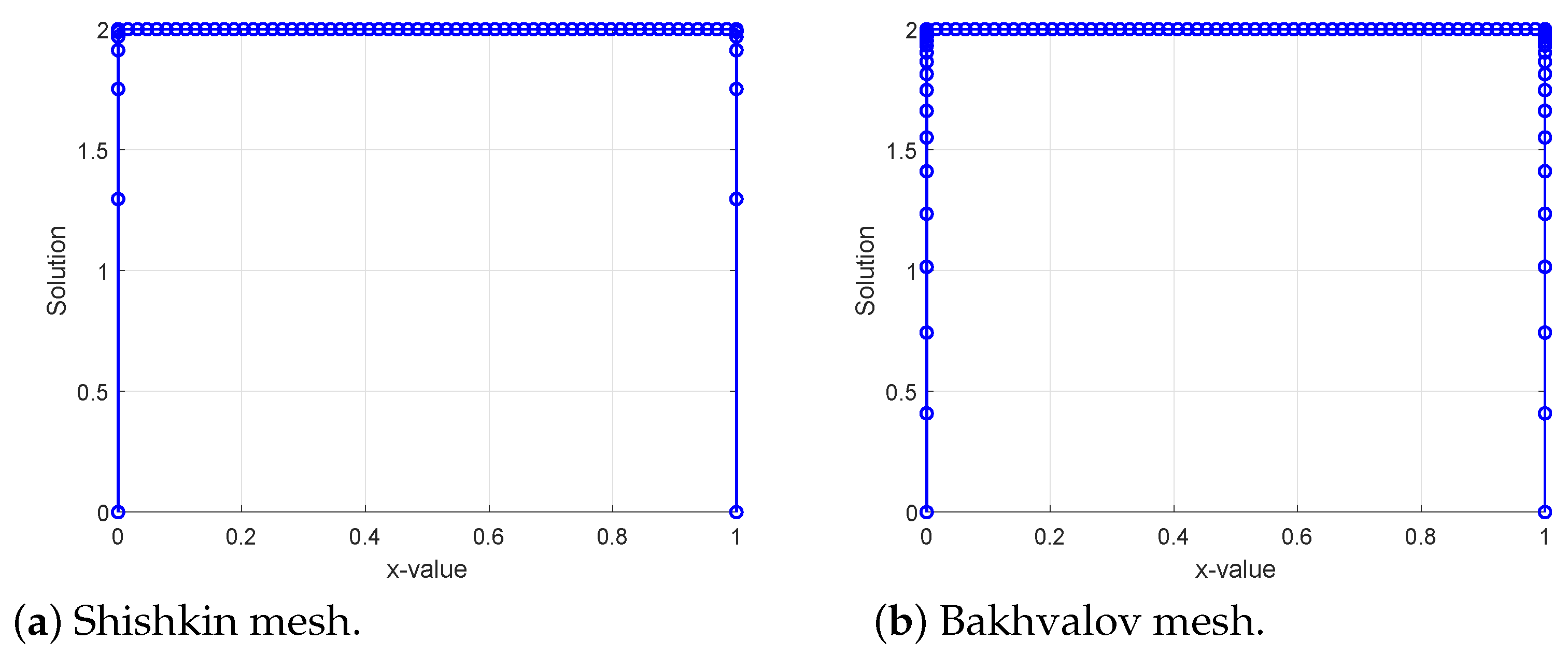
We take the initial guesses $U_0^{\left(0\right)}=u\left(0\right)=0,U_{\mathcal{M}}^{\left(0\right)}=u\left(1\right)=0$ at the boundaries and $U_i^{\left(0\right)}=2$ elsewhere.

Example 2.

Secondly, we consider [22]

$$\left\{\begin{array}{c}-{\epsilon }^2{u}^{″}\left(x\right)+(u^2+u-3.75)(u-0.5)(u+2-cosx)=0,x\in [0,1],\hfill \\ u\left(0\right)=0,u\left(1\right)=0.\hfill \end{array}\right.$$

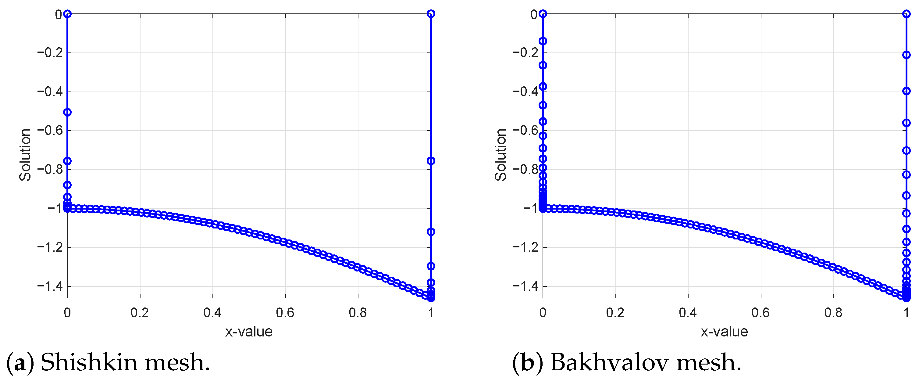
We take the initial guesses $U_0^{\left(0\right)}=u\left(0\right)=0,U_{\mathcal{M}}^{\left(0\right)}=u\left(1\right)=0$ at the boundaries and $U_i^{\left(0\right)}=cosx-2$ elsewhere.

Example 3.

Lastly, we consider [8]

$$\left\{\begin{array}{c}-{\epsilon }^2{u}^{″}\left(x\right)+(u^2-1)(u^2-4)=0,x\in [0,1],\hfill \\ u\left(0\right)={\displaystyle \frac{1}{2}},u\left(1\right)={\displaystyle \frac{1}{2}}.\hfill \end{array}\right.$$

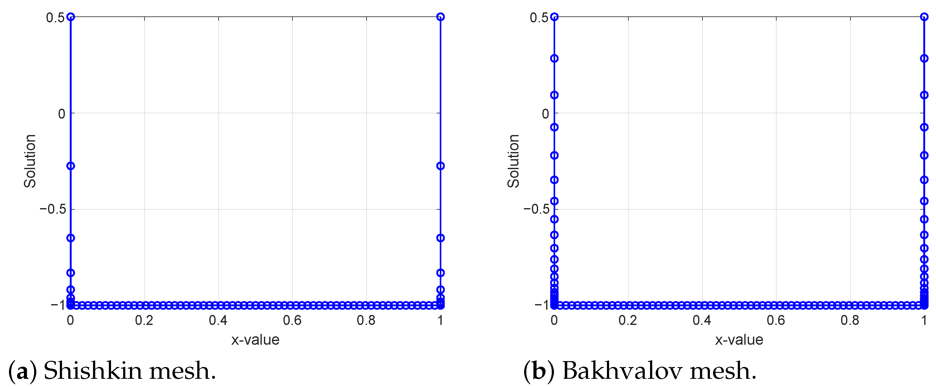
We take initial guess $U_0^{\left(0\right)}=u\left(0\right)=0,U_{\mathcal{M}}^{\left(0\right)}=u\left(1\right)=0$ at the boundaries and $U_i^{\left(0\right)}=-1$ elsewhere. Because there is no exact solution for the test examples, the double mesh approach is used to estimate the maximum point-wise errors prior to and following extrapolations via the formula below

$$\begin{array}{cc}\hfill & e_{\epsilon }^{\mathcal{M}}=\underset{0\le m\le \mathcal{M}}{max}|U^{\mathcal{M}}\left(x_m\right)-U^{2\mathcal{M}}\left(x_m\right)|,\hfill \end{array}$$

$$\begin{array}{cc}\hfill & e_{\epsilon }^{\mathcal{M}}=\underset{0\le m\le \mathcal{M}}{max}|U_{extr}^{\mathcal{M}}\left(x_m\right)-U_{extr}^{2\mathcal{M}}\left(x_m\right)|,\hfill \end{array}$$

where $U^{\mathcal{M}}\left(x_m\right)$ and $U^{2\mathcal{M}}\left(x_{2m}\right)$ are the numerical and the double mesh solutions prior to extrapolation whereas $U_{extr}^{\mathcal{M}}\left(x_m\right)$ and $U_{extr}^{2\mathcal{M}}\left(x_m\right)$ are better-approximated solutions following extrapolation. The maximum point-wise errors and uniform errors are estimated by

$$e_{\epsilon }^{\mathcal{M}}=\underset{0\le m\le \mathcal{M}}{max}{e}_m^{\mathcal{M}}\mathrm{and}{e}^{\mathcal{M}}=\underset{\epsilon }{max}{e}_{\epsilon }^{\mathcal{M}},$$

respectively. The numerical and uniform rates of convergence are calculated using the formulas

$${\rho }_{\epsilon }^{\mathcal{M}}={log}_2\left({\displaystyle \frac{e_{\epsilon }^{\mathcal{M}}}{e_{\epsilon }^{2\mathcal{M}}}}\right)\mathrm{and}{\rho }^{\mathcal{M}}={log}_2\left({\displaystyle \frac{e^{\mathcal{M}}}{e^{2\mathcal{M}}}}\right),$$

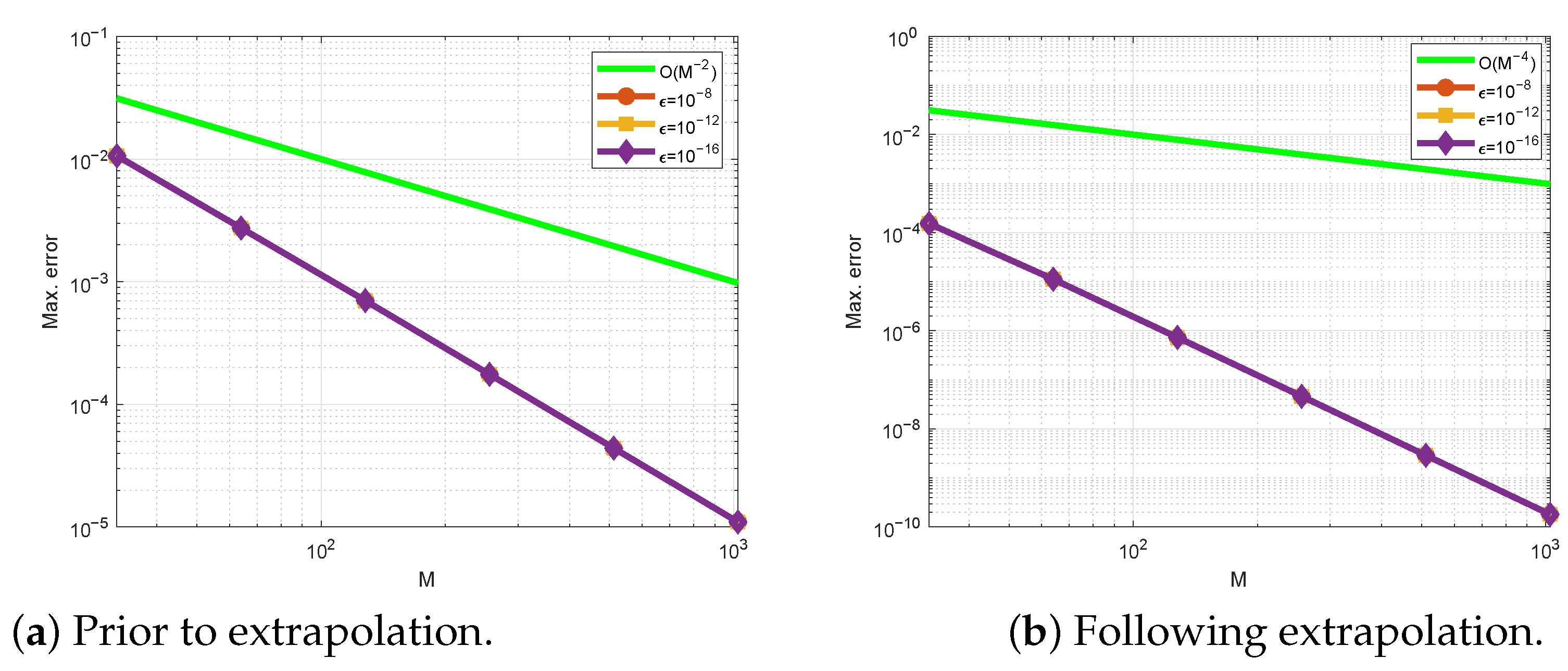
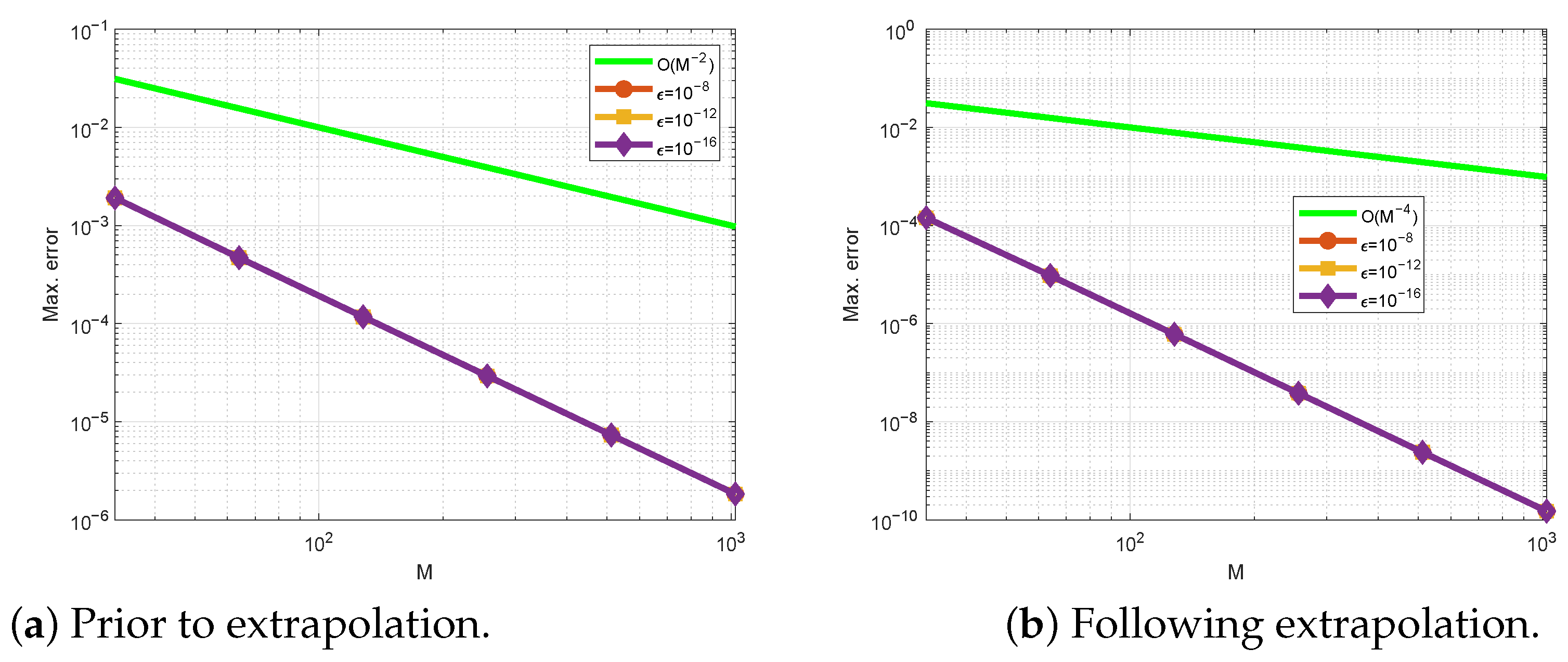
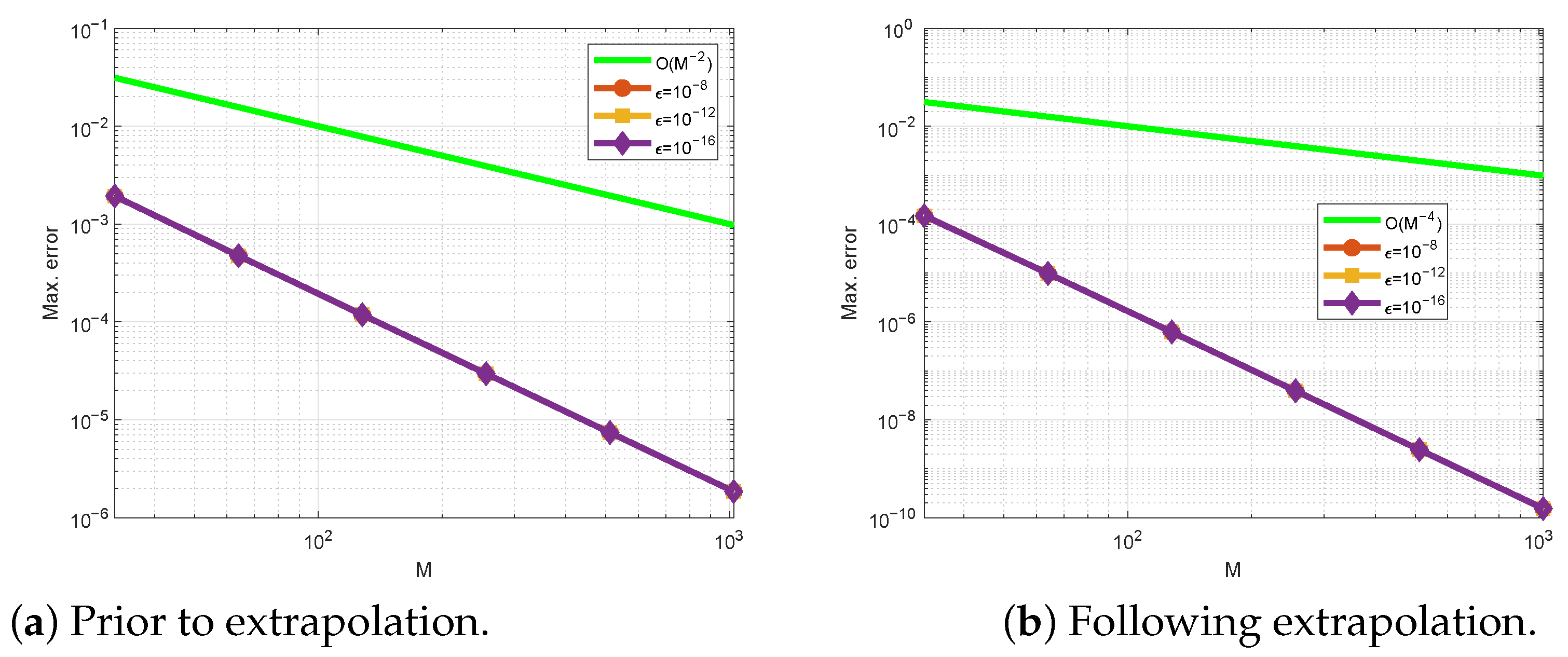
respectively. The numerical solutions using the Shishkin mesh are demonstrated in Table 1, Table 3 and Table 5 for Examples 1, 2, and 3, respectively, prior to and following extrapolations. Similarly, the numerical solutions using the Bakhvalov mesh are depicted in Table 2, Table 4 and Table 6 for Examples 1, 2, and 3, respectively, prior to and following extrapolations. When $\epsilon \to 0$, all the tables show the parameter-uniform convergence of the present method. The Shishkin mesh solution graphs for each example are given on the left-hand side of Figure 1, Figure 2 and Figure 3, respectively. The Bakhvalov mesh solution graphs for each example are given on the right-hand side of Figure 1, Figure 2 and Figure 3, respectively. These right-side figures in Figure 1, Figure 2 and Figure 3 demonstrate that the Bakhvalov mesh condensed more mesh points at boundary layer regions than the Shishkin mesh. For fixed $\epsilon$, the maximum point-wise errors decrease when the mesh points increase. This shows the parameter-uniform convergence. For fixed mesh points, the maximum point-wise error decreases as the values of $\epsilon$ decrease. This shows the stability of the method. In order to observe the rate of convergence, the maximum point-wise errors are plotted in log-log scale on Figure 4, Figure 5 and Figure 6.

Table 1. Shishkin mesh maximum point-wise errors $e_{\epsilon }^{\mathcal{M}},e^{\mathcal{M}}$, and uniform rate of convergence ${\rho }^{\mathcal{M}}$ for Example 1.

${\mathit{\epsilon }}^2\downarrow$	$\mathcal{M}=32$	64	128	256	512	1024	2048
Prior to extrapolation
${10}^{-0}$	4.3426$\times {10}^{-4}$	1.0867$\times {10}^{-4}$	2.7174$\times {10}^{-5}$	6.7939$\times {10}^{-6}$	1.6985$\times {10}^{-6}$	4.2463$\times {10}^{-7}$	1.0616$\times {10}^{-7}$
${10}^{-2}$	2.5484$\times {10}^{-2}$	6.9985$\times {10}^{-3}$	1.7951$\times {10}^{-3}$	4.5501$\times {10}^{-4}$	1.1395$\times {10}^{-4}$	2.8499$\times {10}^{-5}$	7.1261$\times {10}^{-6}$
${10}^{-4}$	5.8047$\times {10}^{-2}$	4.8827$\times {10}^{-2}$	2.4221$\times {10}^{-2}$	8.3884$\times {10}^{-3}$	2.7969$\times {10}^{-3}$	8.7244$\times {10}^{-4}$	2.6464$\times {10}^{-4}$
${10}^{-6}$	5.8047$\times {10}^{-2}$	4.8827$\times {10}^{-2}$	2.4221$\times {10}^{-2}$	8.3884$\times {10}^{-3}$	2.7969$\times {10}^{-3}$	8.7244$\times {10}^{-4}$	2.6464$\times {10}^{-4}$
${10}^{-8}$	5.8047$\times {10}^{-2}$	4.8827$\times {10}^{-2}$	2.4221$\times {10}^{-2}$	8.3884$\times {10}^{-3}$	2.7969$\times {10}^{-3}$	8.7244$\times {10}^{-4}$	2.6464$\times {10}^{-4}$
${10}^{-10}$	5.8047$\times {10}^{-2}$	4.8827$\times {10}^{-2}$	2.4221$\times {10}^{-2}$	8.3884$\times {10}^{-3}$	2.7969$\times {10}^{-3}$	8.7244$\times {10}^{-4}$	2.6464$\times {10}^{-4}$
${10}^{-12}$	5.8047$\times {10}^{-2}$	4.8827$\times {10}^{-2}$	2.4221$\times {10}^{-2}$	8.3884$\times {10}^{-3}$	2.7969$\times {10}^{-3}$	8.7244$\times {10}^{-4}$	2.6464$\times {10}^{-4}$
${10}^{-14}$	5.8047$\times {10}^{-2}$	4.8827$\times {10}^{-2}$	2.4221$\times {10}^{-2}$	8.3884$\times {10}^{-3}$	2.7969$\times {10}^{-3}$	8.7244$\times {10}^{-4}$	2.6464$\times {10}^{-4}$
${10}^{-16}$	5.8047$\times {10}^{-2}$	4.8827$\times {10}^{-2}$	2.4221$\times {10}^{-2}$	8.3884$\times {10}^{-3}$	2.7969$\times {10}^{-3}$	8.7244$\times {10}^{-4}$	2.6464$\times {10}^{-4}$
$e^{\mathcal{M}}$	5.8047$\times {10}^{-2}$	4.8827$\times {10}^{-2}$	2.4221$\times {10}^{-2}$	8.3884$\times {10}^{-3}$	2.7969$\times {10}^{-3}$	8.7244$\times {10}^{-4}$	2.6464$\times {10}^{-4}$
${\rho }^{\mathcal{M}}$	0.2495	1.0114	1.5298	1.5846	1.6807	1.7210	-
Following extrapolation
${10}^{-0}$	1.4048$\times {10}^{-7}$	8.7941$\times {10}^{-9}$	5.4991$\times {10}^{-10}$	3.4311$\times {10}^{-11}$	2.9494$\times {10}^{-12}$	3.1573$\times {10}^{-12}$	8.0314$\times {10}^{-12}$
${10}^{-2}$	8.3657$\times {10}^{-4}$	6.0600$\times {10}^{-5}$	4.1759$\times {10}^{-6}$	2.6378$\times {10}^{-7}$	1.6530$\times {10}^{-8}$	1.0341$\times {10}^{-9}$	6.4760$\times {10}^{-11}$
${10}^{-4}$	5.3488$\times {10}^{-3}$	3.2477$\times {10}^{-3}$	7.5775$\times {10}^{-4}$	9.2391$\times {10}^{-5}$	9.9244$\times {10}^{-6}$	9.7022$\times {10}^{-7}$	8.9222$\times {10}^{-8}$
${10}^{-6}$	5.3488$\times {10}^{-3}$	3.2477$\times {10}^{-3}$	7.5775$\times {10}^{-4}$	9.2391$\times {10}^{-5}$	9.9244$\times {10}^{-6}$	9.7022$\times {10}^{-7}$	8.9222$\times {10}^{-8}$
${10}^{-8}$	5.3488$\times {10}^{-3}$	3.2477$\times {10}^{-3}$	7.5775$\times {10}^{-4}$	9.2391$\times {10}^{-5}$	9.9244$\times {10}^{-6}$	9.7022$\times {10}^{-7}$	8.9222$\times {10}^{-8}$
${10}^{-10}$	5.3488$\times {10}^{-3}$	3.2477$\times {10}^{-3}$	7.5775$\times {10}^{-4}$	9.2391$\times {10}^{-5}$	9.9244$\times {10}^{-6}$	9.7022$\times {10}^{-7}$	8.9222$\times {10}^{-8}$
${10}^{-12}$	5.3488$\times {10}^{-3}$	3.2477$\times {10}^{-3}$	7.5775$\times {10}^{-4}$	9.2391$\times {10}^{-5}$	9.9244$\times {10}^{-6}$	9.7022$\times {10}^{-7}$	8.9222$\times {10}^{-8}$
${10}^{-14}$	5.3488$\times {10}^{-3}$	3.2477$\times {10}^{-3}$	7.5775$\times {10}^{-4}$	9.2391$\times {10}^{-5}$	9.9244$\times {10}^{-6}$	9.7022$\times {10}^{-7}$	8.9222$\times {10}^{-8}$
${10}^{-16}$	5.3488$\times {10}^{-3}$	3.2477$\times {10}^{-3}$	7.5775$\times {10}^{-4}$	9.2391$\times {10}^{-5}$	9.9244$\times {10}^{-6}$	9.7022$\times {10}^{-7}$	8.9222$\times {10}^{-8}$
$e^{2\mathcal{M}}$	5.3488$\times {10}^{-3}$	3.2477$\times {10}^{-3}$	7.5775$\times {10}^{-4}$	9.2391$\times {10}^{-5}$	9.9244$\times {10}^{-6}$	9.7022$\times {10}^{-7}$	8.9222$\times {10}^{-8}$
${\rho }^{2\mathcal{M}}$	0.7198	2.0996	3.0359	3.2187	3.3546	3.4428	-

Table 1. Shishkin mesh maximum point-wise errors $e_{\epsilon }^{\mathcal{M}},e^{\mathcal{M}}$, and uniform rate of convergence ${\rho }^{\mathcal{M}}$ for Example 1.

${\mathit{\epsilon }}^2\downarrow$	$\mathcal{M}=32$	64	128	256	512	1024	2048
Prior to extrapolation
${10}^{-0}$	4.3426$\times {10}^{-4}$	1.0867$\times {10}^{-4}$	2.7174$\times {10}^{-5}$	6.7939$\times {10}^{-6}$	1.6985$\times {10}^{-6}$	4.2463$\times {10}^{-7}$	1.0616$\times {10}^{-7}$
${10}^{-2}$	2.5484$\times {10}^{-2}$	6.9985$\times {10}^{-3}$	1.7951$\times {10}^{-3}$	4.5501$\times {10}^{-4}$	1.1395$\times {10}^{-4}$	2.8499$\times {10}^{-5}$	7.1261$\times {10}^{-6}$
${10}^{-4}$	5.8047$\times {10}^{-2}$	4.8827$\times {10}^{-2}$	2.4221$\times {10}^{-2}$	8.3884$\times {10}^{-3}$	2.7969$\times {10}^{-3}$	8.7244$\times {10}^{-4}$	2.6464$\times {10}^{-4}$
${10}^{-6}$	5.8047$\times {10}^{-2}$	4.8827$\times {10}^{-2}$	2.4221$\times {10}^{-2}$	8.3884$\times {10}^{-3}$	2.7969$\times {10}^{-3}$	8.7244$\times {10}^{-4}$	2.6464$\times {10}^{-4}$
${10}^{-8}$	5.8047$\times {10}^{-2}$	4.8827$\times {10}^{-2}$	2.4221$\times {10}^{-2}$	8.3884$\times {10}^{-3}$	2.7969$\times {10}^{-3}$	8.7244$\times {10}^{-4}$	2.6464$\times {10}^{-4}$
${10}^{-10}$	5.8047$\times {10}^{-2}$	4.8827$\times {10}^{-2}$	2.4221$\times {10}^{-2}$	8.3884$\times {10}^{-3}$	2.7969$\times {10}^{-3}$	8.7244$\times {10}^{-4}$	2.6464$\times {10}^{-4}$
${10}^{-12}$	5.8047$\times {10}^{-2}$	4.8827$\times {10}^{-2}$	2.4221$\times {10}^{-2}$	8.3884$\times {10}^{-3}$	2.7969$\times {10}^{-3}$	8.7244$\times {10}^{-4}$	2.6464$\times {10}^{-4}$
${10}^{-14}$	5.8047$\times {10}^{-2}$	4.8827$\times {10}^{-2}$	2.4221$\times {10}^{-2}$	8.3884$\times {10}^{-3}$	2.7969$\times {10}^{-3}$	8.7244$\times {10}^{-4}$	2.6464$\times {10}^{-4}$
${10}^{-16}$	5.8047$\times {10}^{-2}$	4.8827$\times {10}^{-2}$	2.4221$\times {10}^{-2}$	8.3884$\times {10}^{-3}$	2.7969$\times {10}^{-3}$	8.7244$\times {10}^{-4}$	2.6464$\times {10}^{-4}$
$e^{\mathcal{M}}$	5.8047$\times {10}^{-2}$	4.8827$\times {10}^{-2}$	2.4221$\times {10}^{-2}$	8.3884$\times {10}^{-3}$	2.7969$\times {10}^{-3}$	8.7244$\times {10}^{-4}$	2.6464$\times {10}^{-4}$
${\rho }^{\mathcal{M}}$	0.2495	1.0114	1.5298	1.5846	1.6807	1.7210	-
Following extrapolation
${10}^{-0}$	1.4048$\times {10}^{-7}$	8.7941$\times {10}^{-9}$	5.4991$\times {10}^{-10}$	3.4311$\times {10}^{-11}$	2.9494$\times {10}^{-12}$	3.1573$\times {10}^{-12}$	8.0314$\times {10}^{-12}$
${10}^{-2}$	8.3657$\times {10}^{-4}$	6.0600$\times {10}^{-5}$	4.1759$\times {10}^{-6}$	2.6378$\times {10}^{-7}$	1.6530$\times {10}^{-8}$	1.0341$\times {10}^{-9}$	6.4760$\times {10}^{-11}$
${10}^{-4}$	5.3488$\times {10}^{-3}$	3.2477$\times {10}^{-3}$	7.5775$\times {10}^{-4}$	9.2391$\times {10}^{-5}$	9.9244$\times {10}^{-6}$	9.7022$\times {10}^{-7}$	8.9222$\times {10}^{-8}$
${10}^{-6}$	5.3488$\times {10}^{-3}$	3.2477$\times {10}^{-3}$	7.5775$\times {10}^{-4}$	9.2391$\times {10}^{-5}$	9.9244$\times {10}^{-6}$	9.7022$\times {10}^{-7}$	8.9222$\times {10}^{-8}$
${10}^{-8}$	5.3488$\times {10}^{-3}$	3.2477$\times {10}^{-3}$	7.5775$\times {10}^{-4}$	9.2391$\times {10}^{-5}$	9.9244$\times {10}^{-6}$	9.7022$\times {10}^{-7}$	8.9222$\times {10}^{-8}$
${10}^{-10}$	5.3488$\times {10}^{-3}$	3.2477$\times {10}^{-3}$	7.5775$\times {10}^{-4}$	9.2391$\times {10}^{-5}$	9.9244$\times {10}^{-6}$	9.7022$\times {10}^{-7}$	8.9222$\times {10}^{-8}$
${10}^{-12}$	5.3488$\times {10}^{-3}$	3.2477$\times {10}^{-3}$	7.5775$\times {10}^{-4}$	9.2391$\times {10}^{-5}$	9.9244$\times {10}^{-6}$	9.7022$\times {10}^{-7}$	8.9222$\times {10}^{-8}$
${10}^{-14}$	5.3488$\times {10}^{-3}$	3.2477$\times {10}^{-3}$	7.5775$\times {10}^{-4}$	9.2391$\times {10}^{-5}$	9.9244$\times {10}^{-6}$	9.7022$\times {10}^{-7}$	8.9222$\times {10}^{-8}$
${10}^{-16}$	5.3488$\times {10}^{-3}$	3.2477$\times {10}^{-3}$	7.5775$\times {10}^{-4}$	9.2391$\times {10}^{-5}$	9.9244$\times {10}^{-6}$	9.7022$\times {10}^{-7}$	8.9222$\times {10}^{-8}$
$e^{2\mathcal{M}}$	5.3488$\times {10}^{-3}$	3.2477$\times {10}^{-3}$	7.5775$\times {10}^{-4}$	9.2391$\times {10}^{-5}$	9.9244$\times {10}^{-6}$	9.7022$\times {10}^{-7}$	8.9222$\times {10}^{-8}$
${\rho }^{2\mathcal{M}}$	0.7198	2.0996	3.0359	3.2187	3.3546	3.4428	-

Table 2. Bakhvalov mesh maximum point-wise errors $e_{\epsilon }^{\mathcal{M}},e^{\mathcal{M}}$, and rate of convergence ${\rho }^{\mathcal{M}}$ for Example 1.

${\mathit{\epsilon }}^2\downarrow$	$\mathcal{M}=32$	64	128	256	512	1024	2048
Prior to extrapolation
${10}^{-4}$	1.0403$\times {10}^{-2}$	2.6788$\times {10}^{-3}$	6.8783$\times {10}^{-4}$	1.7227$\times {10}^{-4}$	4.3101$\times {10}^{-5}$	1.0779$\times {10}^{-5}$	2.6947$\times {10}^{-6}$
${10}^{-6}$	1.0604$\times {10}^{-2}$	2.7320$\times {10}^{-3}$	7.0010$\times {10}^{-4}$	1.7534$\times {10}^{-4}$	4.3895$\times {10}^{-5}$	1.0975$\times {10}^{-5}$	2.7440$\times {10}^{-6}$
${10}^{-8}$	1.0625$\times {10}^{-2}$	2.7374$\times {10}^{-3}$	7.0132$\times {10}^{-4}$	1.7565$\times {10}^{-4}$	4.3974$\times {10}^{-5}$	1.0995$\times {10}^{-5}$	2.7489$\times {10}^{-6}$
${10}^{-10}$	1.0627$\times {10}^{-2}$	2.7379$\times {10}^{-3}$	7.0145$\times {10}^{-4}$	1.7568$\times {10}^{-4}$	4.3982$\times {10}^{-5}$	1.0997$\times {10}^{-5}$	2.7494$\times {10}^{-6}$
${10}^{-12}$	1.0627$\times {10}^{-2}$	2.7380$\times {10}^{-3}$	7.0146$\times {10}^{-4}$	1.7568$\times {10}^{-4}$	4.3983$\times {10}^{-5}$	1.0997$\times {10}^{-5}$	2.7495$\times {10}^{-6}$
${10}^{-14}$	1.0627$\times {10}^{-2}$	2.7380$\times {10}^{-3}$	7.0146$\times {10}^{-4}$	1.7568$\times {10}^{-4}$	4.3983$\times {10}^{-5}$	1.0997$\times {10}^{-5}$	2.7495$\times {10}^{-6}$
${10}^{-16}$	1.0627$\times {10}^{-2}$	2.7380$\times {10}^{-3}$	7.0146$\times {10}^{-4}$	1.7568$\times {10}^{-4}$	4.3983$\times {10}^{-5}$	1.0997$\times {10}^{-5}$	2.7495$\times {10}^{-6}$
$e^{\mathcal{M}}$	1.0627$\times {10}^{-2}$	2.7380$\times {10}^{-3}$	7.0146$\times {10}^{-4}$	1.7568$\times {10}^{-4}$	4.3983$\times {10}^{-5}$	1.0997$\times {10}^{-5}$	2.7495$\times {10}^{-6}$
${\rho }^{\mathcal{M}}$	1.9565	1.9647	1.9974	1.9979	1.9998	1.9999	-
Following extrapolation
${10}^{-4}$	1.4824$\times {10}^{-4}$	1.0818$\times {10}^{-5}$	7.0309$\times {10}^{-7}$	4.4376$\times {10}^{-8}$	2.7810$\times {10}^{-9}$	1.7402$\times {10}^{-10}$	1.1803$\times {10}^{-11}$
${10}^{-6}$	1.5303$\times {10}^{-4}$	1.1201$\times {10}^{-5}$	7.2859$\times {10}^{-7}$	4.5995$\times {10}^{-8}$	2.8835$\times {10}^{-9}$	1.8049$\times {10}^{-10}$	1.1947$\times {10}^{-11}$
${10}^{-8}$	1.5351$\times {10}^{-4}$	1.1240$\times {10}^{-5}$	7.3117$\times {10}^{-7}$	4.6159$\times {10}^{-8}$	2.8940$\times {10}^{-9}$	1.8100$\times {10}^{-10}$	1.2006$\times {10}^{-11}$
${10}^{-10}$	1.5356$\times {10}^{-4}$	1.1244$\times {10}^{-5}$	7.3143$\times {10}^{-7}$	4.6175$\times {10}^{-8}$	2.8952$\times {10}^{-9}$	1.8158$\times {10}^{-10}$	1.2008$\times {10}^{-11}$
${10}^{-12}$	1.5357$\times {10}^{-4}$	1.1244$\times {10}^{-5}$	7.3145$\times {10}^{-7}$	4.6177$\times {10}^{-8}$	2.8952$\times {10}^{-9}$	1.8165$\times {10}^{-10}$	1.2092$\times {10}^{-11}$
${10}^{-14}$	1.5357$\times {10}^{-4}$	1.1244$\times {10}^{-5}$	7.3146$\times {10}^{-7}$	4.6177$\times {10}^{-8}$	2.8952$\times {10}^{-9}$	1.8165$\times {10}^{-10}$	1.2098$\times {10}^{-11}$
${10}^{-16}$	1.5357$\times {10}^{-4}$	1.1244$\times {10}^{-5}$	7.3147$\times {10}^{-7}$	4.6177$\times {10}^{-8}$	2.8952$\times {10}^{-9}$	1.8165$\times {10}^{-10}$	1.2251$\times {10}^{-11}$
$e^{2\mathcal{M}}$	1.5357$\times {10}^{-4}$	1.1244$\times {10}^{-5}$	7.3147$\times {10}^{-7}$	4.6177$\times {10}^{-8}$	2.8952$\times {10}^{-9}$	1.8115$\times {10}^{-10}$	1.2251$\times {10}^{-11}$
${\rho }^{2\mathcal{M}}$	3.7717	3.9422	3.9856	3.9954	3.9984	3.9992	-

Table 2. Bakhvalov mesh maximum point-wise errors $e_{\epsilon }^{\mathcal{M}},e^{\mathcal{M}}$, and rate of convergence ${\rho }^{\mathcal{M}}$ for Example 1.

${\mathit{\epsilon }}^2\downarrow$	$\mathcal{M}=32$	64	128	256	512	1024	2048
Prior to extrapolation
${10}^{-4}$	1.0403$\times {10}^{-2}$	2.6788$\times {10}^{-3}$	6.8783$\times {10}^{-4}$	1.7227$\times {10}^{-4}$	4.3101$\times {10}^{-5}$	1.0779$\times {10}^{-5}$	2.6947$\times {10}^{-6}$
${10}^{-6}$	1.0604$\times {10}^{-2}$	2.7320$\times {10}^{-3}$	7.0010$\times {10}^{-4}$	1.7534$\times {10}^{-4}$	4.3895$\times {10}^{-5}$	1.0975$\times {10}^{-5}$	2.7440$\times {10}^{-6}$
${10}^{-8}$	1.0625$\times {10}^{-2}$	2.7374$\times {10}^{-3}$	7.0132$\times {10}^{-4}$	1.7565$\times {10}^{-4}$	4.3974$\times {10}^{-5}$	1.0995$\times {10}^{-5}$	2.7489$\times {10}^{-6}$
${10}^{-10}$	1.0627$\times {10}^{-2}$	2.7379$\times {10}^{-3}$	7.0145$\times {10}^{-4}$	1.7568$\times {10}^{-4}$	4.3982$\times {10}^{-5}$	1.0997$\times {10}^{-5}$	2.7494$\times {10}^{-6}$
${10}^{-12}$	1.0627$\times {10}^{-2}$	2.7380$\times {10}^{-3}$	7.0146$\times {10}^{-4}$	1.7568$\times {10}^{-4}$	4.3983$\times {10}^{-5}$	1.0997$\times {10}^{-5}$	2.7495$\times {10}^{-6}$
${10}^{-14}$	1.0627$\times {10}^{-2}$	2.7380$\times {10}^{-3}$	7.0146$\times {10}^{-4}$	1.7568$\times {10}^{-4}$	4.3983$\times {10}^{-5}$	1.0997$\times {10}^{-5}$	2.7495$\times {10}^{-6}$
${10}^{-16}$	1.0627$\times {10}^{-2}$	2.7380$\times {10}^{-3}$	7.0146$\times {10}^{-4}$	1.7568$\times {10}^{-4}$	4.3983$\times {10}^{-5}$	1.0997$\times {10}^{-5}$	2.7495$\times {10}^{-6}$
$e^{\mathcal{M}}$	1.0627$\times {10}^{-2}$	2.7380$\times {10}^{-3}$	7.0146$\times {10}^{-4}$	1.7568$\times {10}^{-4}$	4.3983$\times {10}^{-5}$	1.0997$\times {10}^{-5}$	2.7495$\times {10}^{-6}$
${\rho }^{\mathcal{M}}$	1.9565	1.9647	1.9974	1.9979	1.9998	1.9999	-
Following extrapolation
${10}^{-4}$	1.4824$\times {10}^{-4}$	1.0818$\times {10}^{-5}$	7.0309$\times {10}^{-7}$	4.4376$\times {10}^{-8}$	2.7810$\times {10}^{-9}$	1.7402$\times {10}^{-10}$	1.1803$\times {10}^{-11}$
${10}^{-6}$	1.5303$\times {10}^{-4}$	1.1201$\times {10}^{-5}$	7.2859$\times {10}^{-7}$	4.5995$\times {10}^{-8}$	2.8835$\times {10}^{-9}$	1.8049$\times {10}^{-10}$	1.1947$\times {10}^{-11}$
${10}^{-8}$	1.5351$\times {10}^{-4}$	1.1240$\times {10}^{-5}$	7.3117$\times {10}^{-7}$	4.6159$\times {10}^{-8}$	2.8940$\times {10}^{-9}$	1.8100$\times {10}^{-10}$	1.2006$\times {10}^{-11}$
${10}^{-10}$	1.5356$\times {10}^{-4}$	1.1244$\times {10}^{-5}$	7.3143$\times {10}^{-7}$	4.6175$\times {10}^{-8}$	2.8952$\times {10}^{-9}$	1.8158$\times {10}^{-10}$	1.2008$\times {10}^{-11}$
${10}^{-12}$	1.5357$\times {10}^{-4}$	1.1244$\times {10}^{-5}$	7.3145$\times {10}^{-7}$	4.6177$\times {10}^{-8}$	2.8952$\times {10}^{-9}$	1.8165$\times {10}^{-10}$	1.2092$\times {10}^{-11}$
${10}^{-14}$	1.5357$\times {10}^{-4}$	1.1244$\times {10}^{-5}$	7.3146$\times {10}^{-7}$	4.6177$\times {10}^{-8}$	2.8952$\times {10}^{-9}$	1.8165$\times {10}^{-10}$	1.2098$\times {10}^{-11}$
${10}^{-16}$	1.5357$\times {10}^{-4}$	1.1244$\times {10}^{-5}$	7.3147$\times {10}^{-7}$	4.6177$\times {10}^{-8}$	2.8952$\times {10}^{-9}$	1.8165$\times {10}^{-10}$	1.2251$\times {10}^{-11}$
$e^{2\mathcal{M}}$	1.5357$\times {10}^{-4}$	1.1244$\times {10}^{-5}$	7.3147$\times {10}^{-7}$	4.6177$\times {10}^{-8}$	2.8952$\times {10}^{-9}$	1.8115$\times {10}^{-10}$	1.2251$\times {10}^{-11}$
${\rho }^{2\mathcal{M}}$	3.7717	3.9422	3.9856	3.9954	3.9984	3.9992	-

Table 3. Shishkin mesh maximum point-wise errors $e_{\epsilon }^{\mathcal{M}},e^{\mathcal{M}}$, and uniform rate of convergence ${\rho }^{\mathcal{M}}$ for Example 2.

${\mathit{\epsilon }}^2\downarrow$	$\mathcal{M}=32$	64	128	256	512	1024	2048
Prior to extrapolation
${10}^{-0}$	1.3760$\times {10}^{-4}$	3.4416$\times {10}^{-5}$	8.6050$\times {10}^{-6}$	2.1514$\times {10}^{-6}$	5.3784$\times {10}^{-7}$	1.3446$\times {10}^{-7}$	3.3615$\times {10}^{-8}$
${10}^{-2}$	8.9219$\times {10}^{-3}$	2.4005$\times {10}^{-3}$	6.1294$\times {10}^{-4}$	1.5372$\times {10}^{-4}$	3.8494$\times {10}^{-5}$	9.6254$\times {10}^{-6}$	2.4065$\times {10}^{-6}$
${10}^{-4}$	3.9016$\times {10}^{-2}$	2.2670$\times {10}^{-2}$	8.3904$\times {10}^{-3}$	2.9392$\times {10}^{-3}$	9.5438$\times {10}^{-4}$	2.9561$\times {10}^{-4}$	8.9697$\times {10}^{-5}$
${10}^{-6}$	3.9032$\times {10}^{-2}$	2.2678$\times {10}^{-2}$	8.3937$\times {10}^{-3}$	2.9404$\times {10}^{-3}$	9.5478$\times {10}^{-4}$	2.9573$\times {10}^{-4}$	8.9735$\times {10}^{-5}$
${10}^{-8}$	3.9034$\times {10}^{-2}$	2.2679$\times {10}^{-2}$	8.3940$\times {10}^{-3}$	2.9405$\times {10}^{-3}$	9.5482$\times {10}^{-4}$	2.9575$\times {10}^{-4}$	8.9738$\times {10}^{-5}$
${10}^{-10}$	3.9034$\times {10}^{-2}$	2.2679$\times {10}^{-2}$	8.3941$\times {10}^{-3}$	2.9405$\times {10}^{-3}$	9.5483$\times {10}^{-4}$	2.9575$\times {10}^{-4}$	8.9739$\times {10}^{-5}$
${10}^{-12}$	3.9034$\times {10}^{-2}$	2.2679$\times {10}^{-2}$	8.3941$\times {10}^{-3}$	2.9405$\times {10}^{-3}$	9.5483$\times {10}^{-4}$	2.9575$\times {10}^{-4}$	8.9739$\times {10}^{-5}$
${10}^{-14}$	3.9034$\times {10}^{-2}$	2.2679$\times {10}^{-2}$	8.3941$\times {10}^{-3}$	2.9405$\times {10}^{-3}$	9.5483$\times {10}^{-4}$	2.9575$\times {10}^{-4}$	8.9739$\times {10}^{-5}$
${10}^{-16}$	3.9034$\times {10}^{-2}$	2.2679$\times {10}^{-2}$	8.3941$\times {10}^{-3}$	2.9405$\times {10}^{-3}$	9.5483$\times {10}^{-4}$	2.9575$\times {10}^{-4}$	8.9739$\times {10}^{-5}$
$e^{\mathcal{M}}$	3.9034$\times {10}^{-2}$	2.2679$\times {10}^{-2}$	8.3941$\times {10}^{-3}$	2.9405$\times {10}^{-3}$	9.5483$\times {10}^{-4}$	2.9575$\times {10}^{-4}$	8.9739$\times {10}^{-5}$
${\rho }^{\mathcal{M}}$	0.7834	1.4339	1.5133	1.6227	1.6909	1.7206	-
Following extrapolation
${10}^{-0}$	2.1267$\times {10}^{-8}$	1.3299$\times {10}^{-9}$	8.2978$\times {10}^{-11}$	5.1124$\times {10}^{-12}$	7.5406$\times {10}^{-13}$	1.0995$\times {10}^{-12}$	3.4911$\times {10}^{-12}$
${10}^{-2}$	1.5202$\times {10}^{-4}$	1.0238$\times {10}^{-5}$	6.5247$\times {10}^{-7}$	4.1032$\times {10}^{-8}$	2.5705$\times {10}^{-9}$	1.6099$\times {10}^{-10}$	9.7657$\times {10}^{-12}$
${10}^{-4}$	2.9549$\times {10}^{-3}$	9.0336$\times {10}^{-4}$	1.3656$\times {10}^{-4}$	1.5590$\times {10}^{-5}$	1.5821$\times {10}^{-6}$	1.5307$\times {10}^{-7}$	1.4041$\times {10}^{-8}$
${10}^{-6}$	2.9570$\times {10}^{-3}$	9.0407$\times {10}^{-4}$	1.3669$\times {10}^{-4}$	1.5605$\times {10}^{-5}$	1.5837$\times {10}^{-6}$	1.5322$\times {10}^{-7}$	1.4055$\times {10}^{-8}$
${10}^{-8}$	2.9573$\times {10}^{-3}$	9.0414$\times {10}^{-4}$	1.3670$\times {10}^{-4}$	1.5607$\times {10}^{-5}$	1.5838$\times {10}^{-6}$	1.5324$\times {10}^{-7}$	1.4056$\times {10}^{-8}$
${10}^{-10}$	2.9573$\times {10}^{-3}$	9.0415$\times {10}^{-4}$	1.3670$\times {10}^{-4}$	1.5607$\times {10}^{-5}$	1.5838$\times {10}^{-6}$	1.5324$\times {10}^{-7}$	1.4056$\times {10}^{-8}$
${10}^{-12}$	2.9573$\times {10}^{-3}$	9.0415$\times {10}^{-4}$	1.3670$\times {10}^{-4}$	1.5607$\times {10}^{-5}$	1.5838$\times {10}^{-6}$	1.5324$\times {10}^{-7}$	1.4057$\times {10}^{-8}$
${10}^{-14}$	2.9573$\times {10}^{-3}$	9.0415$\times {10}^{-4}$	1.3670$\times {10}^{-4}$	1.5607$\times {10}^{-5}$	1.5838$\times {10}^{-6}$	1.5324$\times {10}^{-7}$	1.4057$\times {10}^{-8}$
${10}^{-16}$	2.9573$\times {10}^{-3}$	9.0415$\times {10}^{-4}$	1.3670$\times {10}^{-4}$	1.5607$\times {10}^{-5}$	1.5838$\times {10}^{-6}$	1.5324$\times {10}^{-7}$	1.4057$\times {10}^{-8}$
$e^{2\mathcal{M}}$	2.9573$\times {10}^{-3}$	9.0415$\times {10}^{-4}$	1.3670$\times {10}^{-4}$	1.5607$\times {10}^{-5}$	1.5838$\times {10}^{-6}$	1.5324$\times {10}^{-7}$	1.4057$\times {10}^{-8}$
${\rho }^{2\mathcal{M}}$	1.7096	2.7255	3.1307	3.3007	3.3695	3.4464	-
Result in [22]
$e^{\mathcal{M}}$	4.99$\times {10}^{-3}$	1.80$\times {10}^{-3}$	6.37$\times {10}^{-4}$	2.09$\times {10}^{-4}$	6.62$\times {10}^{-5}$	-	-
${\rho }^{\mathcal{M}}$	2.0	1.93	1.99	2.00			-

Table 3. Shishkin mesh maximum point-wise errors $e_{\epsilon }^{\mathcal{M}},e^{\mathcal{M}}$, and uniform rate of convergence ${\rho }^{\mathcal{M}}$ for Example 2.

${\mathit{\epsilon }}^2\downarrow$	$\mathcal{M}=32$	64	128	256	512	1024	2048
Prior to extrapolation
${10}^{-0}$	1.3760$\times {10}^{-4}$	3.4416$\times {10}^{-5}$	8.6050$\times {10}^{-6}$	2.1514$\times {10}^{-6}$	5.3784$\times {10}^{-7}$	1.3446$\times {10}^{-7}$	3.3615$\times {10}^{-8}$
${10}^{-2}$	8.9219$\times {10}^{-3}$	2.4005$\times {10}^{-3}$	6.1294$\times {10}^{-4}$	1.5372$\times {10}^{-4}$	3.8494$\times {10}^{-5}$	9.6254$\times {10}^{-6}$	2.4065$\times {10}^{-6}$
${10}^{-4}$	3.9016$\times {10}^{-2}$	2.2670$\times {10}^{-2}$	8.3904$\times {10}^{-3}$	2.9392$\times {10}^{-3}$	9.5438$\times {10}^{-4}$	2.9561$\times {10}^{-4}$	8.9697$\times {10}^{-5}$
${10}^{-6}$	3.9032$\times {10}^{-2}$	2.2678$\times {10}^{-2}$	8.3937$\times {10}^{-3}$	2.9404$\times {10}^{-3}$	9.5478$\times {10}^{-4}$	2.9573$\times {10}^{-4}$	8.9735$\times {10}^{-5}$
${10}^{-8}$	3.9034$\times {10}^{-2}$	2.2679$\times {10}^{-2}$	8.3940$\times {10}^{-3}$	2.9405$\times {10}^{-3}$	9.5482$\times {10}^{-4}$	2.9575$\times {10}^{-4}$	8.9738$\times {10}^{-5}$
${10}^{-10}$	3.9034$\times {10}^{-2}$	2.2679$\times {10}^{-2}$	8.3941$\times {10}^{-3}$	2.9405$\times {10}^{-3}$	9.5483$\times {10}^{-4}$	2.9575$\times {10}^{-4}$	8.9739$\times {10}^{-5}$
${10}^{-12}$	3.9034$\times {10}^{-2}$	2.2679$\times {10}^{-2}$	8.3941$\times {10}^{-3}$	2.9405$\times {10}^{-3}$	9.5483$\times {10}^{-4}$	2.9575$\times {10}^{-4}$	8.9739$\times {10}^{-5}$
${10}^{-14}$	3.9034$\times {10}^{-2}$	2.2679$\times {10}^{-2}$	8.3941$\times {10}^{-3}$	2.9405$\times {10}^{-3}$	9.5483$\times {10}^{-4}$	2.9575$\times {10}^{-4}$	8.9739$\times {10}^{-5}$
${10}^{-16}$	3.9034$\times {10}^{-2}$	2.2679$\times {10}^{-2}$	8.3941$\times {10}^{-3}$	2.9405$\times {10}^{-3}$	9.5483$\times {10}^{-4}$	2.9575$\times {10}^{-4}$	8.9739$\times {10}^{-5}$
$e^{\mathcal{M}}$	3.9034$\times {10}^{-2}$	2.2679$\times {10}^{-2}$	8.3941$\times {10}^{-3}$	2.9405$\times {10}^{-3}$	9.5483$\times {10}^{-4}$	2.9575$\times {10}^{-4}$	8.9739$\times {10}^{-5}$
${\rho }^{\mathcal{M}}$	0.7834	1.4339	1.5133	1.6227	1.6909	1.7206	-
Following extrapolation
${10}^{-0}$	2.1267$\times {10}^{-8}$	1.3299$\times {10}^{-9}$	8.2978$\times {10}^{-11}$	5.1124$\times {10}^{-12}$	7.5406$\times {10}^{-13}$	1.0995$\times {10}^{-12}$	3.4911$\times {10}^{-12}$
${10}^{-2}$	1.5202$\times {10}^{-4}$	1.0238$\times {10}^{-5}$	6.5247$\times {10}^{-7}$	4.1032$\times {10}^{-8}$	2.5705$\times {10}^{-9}$	1.6099$\times {10}^{-10}$	9.7657$\times {10}^{-12}$
${10}^{-4}$	2.9549$\times {10}^{-3}$	9.0336$\times {10}^{-4}$	1.3656$\times {10}^{-4}$	1.5590$\times {10}^{-5}$	1.5821$\times {10}^{-6}$	1.5307$\times {10}^{-7}$	1.4041$\times {10}^{-8}$
${10}^{-6}$	2.9570$\times {10}^{-3}$	9.0407$\times {10}^{-4}$	1.3669$\times {10}^{-4}$	1.5605$\times {10}^{-5}$	1.5837$\times {10}^{-6}$	1.5322$\times {10}^{-7}$	1.4055$\times {10}^{-8}$
${10}^{-8}$	2.9573$\times {10}^{-3}$	9.0414$\times {10}^{-4}$	1.3670$\times {10}^{-4}$	1.5607$\times {10}^{-5}$	1.5838$\times {10}^{-6}$	1.5324$\times {10}^{-7}$	1.4056$\times {10}^{-8}$
${10}^{-10}$	2.9573$\times {10}^{-3}$	9.0415$\times {10}^{-4}$	1.3670$\times {10}^{-4}$	1.5607$\times {10}^{-5}$	1.5838$\times {10}^{-6}$	1.5324$\times {10}^{-7}$	1.4056$\times {10}^{-8}$
${10}^{-12}$	2.9573$\times {10}^{-3}$	9.0415$\times {10}^{-4}$	1.3670$\times {10}^{-4}$	1.5607$\times {10}^{-5}$	1.5838$\times {10}^{-6}$	1.5324$\times {10}^{-7}$	1.4057$\times {10}^{-8}$
${10}^{-14}$	2.9573$\times {10}^{-3}$	9.0415$\times {10}^{-4}$	1.3670$\times {10}^{-4}$	1.5607$\times {10}^{-5}$	1.5838$\times {10}^{-6}$	1.5324$\times {10}^{-7}$	1.4057$\times {10}^{-8}$
${10}^{-16}$	2.9573$\times {10}^{-3}$	9.0415$\times {10}^{-4}$	1.3670$\times {10}^{-4}$	1.5607$\times {10}^{-5}$	1.5838$\times {10}^{-6}$	1.5324$\times {10}^{-7}$	1.4057$\times {10}^{-8}$
$e^{2\mathcal{M}}$	2.9573$\times {10}^{-3}$	9.0415$\times {10}^{-4}$	1.3670$\times {10}^{-4}$	1.5607$\times {10}^{-5}$	1.5838$\times {10}^{-6}$	1.5324$\times {10}^{-7}$	1.4057$\times {10}^{-8}$
${\rho }^{2\mathcal{M}}$	1.7096	2.7255	3.1307	3.3007	3.3695	3.4464	-
Result in [22]
$e^{\mathcal{M}}$	4.99$\times {10}^{-3}$	1.80$\times {10}^{-3}$	6.37$\times {10}^{-4}$	2.09$\times {10}^{-4}$	6.62$\times {10}^{-5}$	-	-
${\rho }^{\mathcal{M}}$	2.0	1.93	1.99	2.00			-

Table 4. Bakhvalov mesh maximum point-wise errors $e_{\epsilon }^{\mathcal{M}},e^{\mathcal{M}}$, and rate of convergence ${\rho }^{\mathcal{M}}$ for Example 2.

${\mathit{\epsilon }}^2\downarrow$	$\mathcal{M}=32$	64	128	256	512	1024	2048
Prior to extrapolation
${10}^{-4}$	1.8701$\times {10}^{-3}$	4.5984$\times {10}^{-4}$	1.1456$\times {10}^{-4}$	2.8672$\times {10}^{-5}$	7.1660$\times {10}^{-6}$	1.7914$\times {10}^{-6}$	4.4785$\times {10}^{-7}$
${10}^{-6}$	1.9055$\times {10}^{-3}$	4.6843$\times {10}^{-4}$	1.1688$\times {10}^{-4}$	2.9229$\times {10}^{-5}$	7.3053$\times {10}^{-6}$	1.8265$\times {10}^{-6}$	4.5662$\times {10}^{-7}$
${10}^{-8}$	1.9090$\times {10}^{-3}$	4.6929$\times {10}^{-4}$	1.1711$\times {10}^{-4}$	2.9285$\times {10}^{-5}$	7.3196$\times {10}^{-6}$	1.8300$\times {10}^{-6}$	4.5750$\times {10}^{-7}$
${10}^{-10}$	1.9094$\times {10}^{-3}$	4.6937$\times {10}^{-4}$	1.1714$\times {10}^{-4}$	2.9290$\times {10}^{-5}$	7.3210$\times {10}^{-6}$	1.8304$\times {10}^{-6}$	4.5759$\times {10}^{-7}$
${10}^{-12}$	1.9094$\times {10}^{-3}$	4.6938$\times {10}^{-4}$	1.1714$\times {10}^{-4}$	2.9291$\times {10}^{-5}$	7.3212$\times {10}^{-6}$	1.8304$\times {10}^{-6}$	4.5760$\times {10}^{-7}$
${10}^{-14}$	1.9094$\times {10}^{-3}$	4.6938$\times {10}^{-4}$	1.1714$\times {10}^{-4}$	2.9291$\times {10}^{-5}$	7.3212$\times {10}^{-6}$	1.8304$\times {10}^{-6}$	4.5760$\times {10}^{-7}$
${10}^{-16}$	1.9094$\times {10}^{-3}$	4.6938$\times {10}^{-4}$	1.1714$\times {10}^{-4}$	2.9291$\times {10}^{-5}$	7.3212$\times {10}^{-6}$	1.8304$\times {10}^{-6}$	4.5760$\times {10}^{-7}$
$e^{\mathcal{M}}$	1.9094$\times {10}^{-3}$	4.6938$\times {10}^{-4}$	1.1714$\times {10}^{-4}$	2.9291$\times {10}^{-5}$	7.3212$\times {10}^{-6}$	1.8304$\times {10}^{-6}$	4.5760$\times {10}^{-7}$
${\rho }^{\mathcal{M}}$	2.0243	2.0025	1.9997	2.0003	1.9999	2.0000	-
Following extrapolation
${10}^{-4}$	1.3854$\times {10}^{-4}$	9.1729$\times {10}^{-6}$	5.8314$\times {10}^{-7}$	3.6578$\times {10}^{-8}$	2.2887$\times {10}^{-9}$	1.1115$\times {10}^{-10}$	1.0100$\times {10}^{-11}$
${10}^{-6}$	1.4316$\times {10}^{-4}$	9.4932$\times {10}^{-6}$	6.0432$\times {10}^{-7}$	3.7903$\times {10}^{-8}$	2.3714$\times {10}^{-9}$	1.4844$\times {10}^{-10}$	1.0101$\times {10}^{-11}$
${10}^{-8}$	1.4363$\times {10}^{-4}$	9.5256$\times {10}^{-6}$	6.0646$\times {10}^{-7}$	3.8038$\times {10}^{-8}$	2.3799$\times {10}^{-9}$	1.4859$\times {10}^{-10}$	1.0102$\times {10}^{-11}$
${10}^{-10}$	1.4367$\times {10}^{-4}$	9.5288$\times {10}^{-6}$	6.0668$\times {10}^{-7}$	3.8052$\times {10}^{-8}$	2.3807$\times {10}^{-9}$	1.4934$\times {10}^{-10}$	1.0103$\times {10}^{-11}$
${10}^{-12}$	1.4368$\times {10}^{-4}$	9.5292$\times {10}^{-6}$	6.0670$\times {10}^{-7}$	3.8053$\times {10}^{-8}$	2.3808$\times {10}^{-9}$	1.4986$\times {10}^{-10}$	1.0120$\times {10}^{-11}$
${10}^{-14}$	1.4368$\times {10}^{-4}$	9.5292$\times {10}^{-6}$	6.0670$\times {10}^{-7}$	3.8053$\times {10}^{-8}$	2.3809$\times {10}^{-9}$	1.4994$\times {10}^{-10}$	1.0120$\times {10}^{-11}$
${10}^{-16}$	1.4368$\times {10}^{-4}$	9.5292$\times {10}^{-6}$	6.0670$\times {10}^{-7}$	3.8053$\times {10}^{-8}$	2.3809$\times {10}^{-9}$	1.4994$\times {10}^{-10}$	1.0120$\times {10}^{-11}$
$e^{2\mathcal{M}}$	1.4368$\times {10}^{-4}$	9.5292$\times {10}^{-6}$	6.0670$\times {10}^{-7}$	3.8053$\times {10}^{-8}$	2.3809$\times {10}^{-9}$	1.4994$\times {10}^{-10}$	1.0120$\times {10}^{-11}$
${\rho }^{2\mathcal{M}}$	3.9144	3.9733	3.9949	3.9984	3.9890	3.8891	-
Result in [22]
$e^{\mathcal{M}}$	1.85$\times {10}^{-3}$	4.63$\times {10}^{-4}$	1.16$\times {10}^{-4}$	2.90$\times {10}^{-5}$	7.24$\times {10}^{-6}$	-	-
${\rho }^{\mathcal{M}}$	2.000	2.0000	2.0000	2.0000	2.0000	2.0000	-

Table 4. Bakhvalov mesh maximum point-wise errors $e_{\epsilon }^{\mathcal{M}},e^{\mathcal{M}}$, and rate of convergence ${\rho }^{\mathcal{M}}$ for Example 2.

${\mathit{\epsilon }}^2\downarrow$	$\mathcal{M}=32$	64	128	256	512	1024	2048
Prior to extrapolation
${10}^{-4}$	1.8701$\times {10}^{-3}$	4.5984$\times {10}^{-4}$	1.1456$\times {10}^{-4}$	2.8672$\times {10}^{-5}$	7.1660$\times {10}^{-6}$	1.7914$\times {10}^{-6}$	4.4785$\times {10}^{-7}$
${10}^{-6}$	1.9055$\times {10}^{-3}$	4.6843$\times {10}^{-4}$	1.1688$\times {10}^{-4}$	2.9229$\times {10}^{-5}$	7.3053$\times {10}^{-6}$	1.8265$\times {10}^{-6}$	4.5662$\times {10}^{-7}$
${10}^{-8}$	1.9090$\times {10}^{-3}$	4.6929$\times {10}^{-4}$	1.1711$\times {10}^{-4}$	2.9285$\times {10}^{-5}$	7.3196$\times {10}^{-6}$	1.8300$\times {10}^{-6}$	4.5750$\times {10}^{-7}$
${10}^{-10}$	1.9094$\times {10}^{-3}$	4.6937$\times {10}^{-4}$	1.1714$\times {10}^{-4}$	2.9290$\times {10}^{-5}$	7.3210$\times {10}^{-6}$	1.8304$\times {10}^{-6}$	4.5759$\times {10}^{-7}$
${10}^{-12}$	1.9094$\times {10}^{-3}$	4.6938$\times {10}^{-4}$	1.1714$\times {10}^{-4}$	2.9291$\times {10}^{-5}$	7.3212$\times {10}^{-6}$	1.8304$\times {10}^{-6}$	4.5760$\times {10}^{-7}$
${10}^{-14}$	1.9094$\times {10}^{-3}$	4.6938$\times {10}^{-4}$	1.1714$\times {10}^{-4}$	2.9291$\times {10}^{-5}$	7.3212$\times {10}^{-6}$	1.8304$\times {10}^{-6}$	4.5760$\times {10}^{-7}$
${10}^{-16}$	1.9094$\times {10}^{-3}$	4.6938$\times {10}^{-4}$	1.1714$\times {10}^{-4}$	2.9291$\times {10}^{-5}$	7.3212$\times {10}^{-6}$	1.8304$\times {10}^{-6}$	4.5760$\times {10}^{-7}$
$e^{\mathcal{M}}$	1.9094$\times {10}^{-3}$	4.6938$\times {10}^{-4}$	1.1714$\times {10}^{-4}$	2.9291$\times {10}^{-5}$	7.3212$\times {10}^{-6}$	1.8304$\times {10}^{-6}$	4.5760$\times {10}^{-7}$
${\rho }^{\mathcal{M}}$	2.0243	2.0025	1.9997	2.0003	1.9999	2.0000	-
Following extrapolation
${10}^{-4}$	1.3854$\times {10}^{-4}$	9.1729$\times {10}^{-6}$	5.8314$\times {10}^{-7}$	3.6578$\times {10}^{-8}$	2.2887$\times {10}^{-9}$	1.1115$\times {10}^{-10}$	1.0100$\times {10}^{-11}$
${10}^{-6}$	1.4316$\times {10}^{-4}$	9.4932$\times {10}^{-6}$	6.0432$\times {10}^{-7}$	3.7903$\times {10}^{-8}$	2.3714$\times {10}^{-9}$	1.4844$\times {10}^{-10}$	1.0101$\times {10}^{-11}$
${10}^{-8}$	1.4363$\times {10}^{-4}$	9.5256$\times {10}^{-6}$	6.0646$\times {10}^{-7}$	3.8038$\times {10}^{-8}$	2.3799$\times {10}^{-9}$	1.4859$\times {10}^{-10}$	1.0102$\times {10}^{-11}$
${10}^{-10}$	1.4367$\times {10}^{-4}$	9.5288$\times {10}^{-6}$	6.0668$\times {10}^{-7}$	3.8052$\times {10}^{-8}$	2.3807$\times {10}^{-9}$	1.4934$\times {10}^{-10}$	1.0103$\times {10}^{-11}$
${10}^{-12}$	1.4368$\times {10}^{-4}$	9.5292$\times {10}^{-6}$	6.0670$\times {10}^{-7}$	3.8053$\times {10}^{-8}$	2.3808$\times {10}^{-9}$	1.4986$\times {10}^{-10}$	1.0120$\times {10}^{-11}$
${10}^{-14}$	1.4368$\times {10}^{-4}$	9.5292$\times {10}^{-6}$	6.0670$\times {10}^{-7}$	3.8053$\times {10}^{-8}$	2.3809$\times {10}^{-9}$	1.4994$\times {10}^{-10}$	1.0120$\times {10}^{-11}$
${10}^{-16}$	1.4368$\times {10}^{-4}$	9.5292$\times {10}^{-6}$	6.0670$\times {10}^{-7}$	3.8053$\times {10}^{-8}$	2.3809$\times {10}^{-9}$	1.4994$\times {10}^{-10}$	1.0120$\times {10}^{-11}$
$e^{2\mathcal{M}}$	1.4368$\times {10}^{-4}$	9.5292$\times {10}^{-6}$	6.0670$\times {10}^{-7}$	3.8053$\times {10}^{-8}$	2.3809$\times {10}^{-9}$	1.4994$\times {10}^{-10}$	1.0120$\times {10}^{-11}$
${\rho }^{2\mathcal{M}}$	3.9144	3.9733	3.9949	3.9984	3.9890	3.8891	-
Result in [22]
$e^{\mathcal{M}}$	1.85$\times {10}^{-3}$	4.63$\times {10}^{-4}$	1.16$\times {10}^{-4}$	2.90$\times {10}^{-5}$	7.24$\times {10}^{-6}$	-	-
${\rho }^{\mathcal{M}}$	2.000	2.0000	2.0000	2.0000	2.0000	2.0000	-

Table 5. Shishkin mesh maximum point-wise errors $e_{\epsilon }^{\mathcal{M}},e^{\mathcal{M}}$, and rate of convergence ${\rho }^{\mathcal{M}}$ for Example 3.

${\mathit{\epsilon }}^2\downarrow$	$\mathcal{M}=32$	64	128	256	512	1024	2048
Prior to extrapolation
${10}^{-0}$	1.5293$\times {10}^{-4}$	3.8255$\times {10}^{-5}$	9.5650$\times {10}^{-6}$	2.3913$\times {10}^{-6}$	5.9784$\times {10}^{-7}$	1.4946$\times {10}^{-7}$	3.7365$\times {10}^{-8}$
${10}^{-2}$	9.1407$\times {10}^{-3}$	2.4611$\times {10}^{-3}$	6.2824$\times {10}^{-4}$	1.5756$\times {10}^{-4}$	3.9458$\times {10}^{-5}$	9.8665$\times {10}^{-6}$	2.4668$\times {10}^{-6}$
${10}^{-4}$	4.0045$\times {10}^{-2}$	2.3207$\times {10}^{-2}$	8.5740$\times {10}^{-3}$	3.0038$\times {10}^{-3}$	9.7559$\times {10}^{-4}$	3.0226$\times {10}^{-4}$	9.1705$\times {10}^{-5}$
${10}^{-6}$	4.0045$\times {10}^{-2}$	2.3207$\times {10}^{-2}$	8.5740$\times {10}^{-3}$	3.0038$\times {10}^{-3}$	9.7559$\times {10}^{-4}$	3.0226$\times {10}^{-4}$	9.1705$\times {10}^{-5}$
${10}^{-8}$	4.0045$\times {10}^{-2}$	2.3207$\times {10}^{-2}$	8.5740$\times {10}^{-3}$	3.0038$\times {10}^{-3}$	9.7559$\times {10}^{-4}$	3.0226$\times {10}^{-4}$	9.1705$\times {10}^{-5}$
${10}^{-10}$	4.0045$\times {10}^{-2}$	2.3207$\times {10}^{-2}$	8.5740$\times {10}^{-3}$	3.0038$\times {10}^{-3}$	9.7559$\times {10}^{-4}$	3.0226$\times {10}^{-4}$	9.1705$\times {10}^{-5}$
${10}^{-12}$	4.0045$\times {10}^{-2}$	2.3207$\times {10}^{-2}$	8.5740$\times {10}^{-3}$	3.0038$\times {10}^{-3}$	9.7559$\times {10}^{-4}$	3.0226$\times {10}^{-4}$	9.1705$\times {10}^{-5}$
${10}^{-14}$	4.0045$\times {10}^{-2}$	2.3207$\times {10}^{-2}$	8.5740$\times {10}^{-3}$	3.0038$\times {10}^{-3}$	9.7559$\times {10}^{-4}$	3.0226$\times {10}^{-4}$	9.1705$\times {10}^{-5}$
${10}^{-16}$	4.0045$\times {10}^{-2}$	2.3207$\times {10}^{-2}$	8.5740$\times {10}^{-3}$	3.0038$\times {10}^{-3}$	9.7559$\times {10}^{-4}$	3.0226$\times {10}^{-4}$	9.1705$\times {10}^{-5}$
$e^{\mathcal{M}}$	4.0045$\times {10}^{-2}$	2.3207$\times {10}^{-2}$	8.5740$\times {10}^{-3}$	3.0038$\times {10}^{-3}$	9.7559$\times {10}^{-4}$	3.0226$\times {10}^{-4}$	9.1705$\times {10}^{-5}$
${\rho }^{\mathcal{M}}$	0.7871	1.4365	1.5132	1.6224	1.6905	1.7207	-
Following extrapolation
${10}^{-0}$	2.7972$\times {10}^{-8}$	1.7496$\times {10}^{-9}$	1.0937$\times {10}^{-10}$	6.8847$\times {10}^{-12}$	1.2486$\times {10}^{-13}$	8.3103$\times {10}^{-13}$	1.2486$\times {10}^{-12}$
${10}^{-2}$	1.5622$\times {10}^{-4}$	1.0525$\times {10}^{-5}$	6.7087$\times {10}^{-7}$	4.2190$\times {10}^{-8}$	2.6432$\times {10}^{-9}$	1.6525$\times {10}^{-10}$	1.3473$\times {10}^{-11}$
${10}^{-4}$	3.0259$\times {10}^{-3}$	9.2129$\times {10}^{-4}$	1.3894$\times {10}^{-4}$	1.5862$\times {10}^{-5}$	1.6089$\times {10}^{-6}$	1.5570$\times {10}^{-7}$	1.4282$\times {10}^{-8}$
${10}^{-6}$	3.0259$\times {10}^{-3}$	9.2129$\times {10}^{-4}$	1.3894$\times {10}^{-4}$	1.5862$\times {10}^{-5}$	1.6089$\times {10}^{-6}$	1.5570$\times {10}^{-7}$	1.4282$\times {10}^{-8}$
${10}^{-8}$	3.0259$\times {10}^{-3}$	9.2129$\times {10}^{-4}$	1.3894$\times {10}^{-4}$	1.5862$\times {10}^{-5}$	1.6089$\times {10}^{-6}$	1.5570$\times {10}^{-7}$	1.4282$\times {10}^{-8}$
${10}^{-10}$	3.0259$\times {10}^{-3}$	9.2129$\times {10}^{-4}$	1.3894$\times {10}^{-4}$	1.5862$\times {10}^{-5}$	1.6089$\times {10}^{-6}$	1.5570$\times {10}^{-7}$	1.4282$\times {10}^{-8}$
${10}^{-12}$	3.0259$\times {10}^{-3}$	9.2129$\times {10}^{-4}$	1.3894$\times {10}^{-4}$	1.5862$\times {10}^{-5}$	1.6089$\times {10}^{-6}$	1.5570$\times {10}^{-7}$	1.4282$\times {10}^{-8}$
${10}^{-14}$	3.0259$\times {10}^{-3}$	9.2129$\times {10}^{-4}$	1.3894$\times {10}^{-4}$	1.5862$\times {10}^{-5}$	1.6089$\times {10}^{-6}$	1.5570$\times {10}^{-7}$	1.4282$\times {10}^{-8}$
${10}^{-16}$	3.0259$\times {10}^{-3}$	9.2129$\times {10}^{-4}$	1.3894$\times {10}^{-4}$	1.5862$\times {10}^{-5}$	1.6089$\times {10}^{-6}$	1.5570$\times {10}^{-7}$	1.4282$\times {10}^{-8}$
$e^{2\mathcal{M}}$	3.0259$\times {10}^{-3}$	9.2129$\times {10}^{-4}$	1.3894$\times {10}^{-4}$	1.5862$\times {10}^{-5}$	1.6089$\times {10}^{-6}$	1.5570$\times {10}^{-7}$	1.4282$\times {10}^{-8}$
${\rho }^{2\mathcal{M}}$	1.7156	2.7292	3.1308	3.3014	3.3692	3.4465	-

Table 5. Shishkin mesh maximum point-wise errors $e_{\epsilon }^{\mathcal{M}},e^{\mathcal{M}}$, and rate of convergence ${\rho }^{\mathcal{M}}$ for Example 3.

${\mathit{\epsilon }}^2\downarrow$	$\mathcal{M}=32$	64	128	256	512	1024	2048
Prior to extrapolation
${10}^{-0}$	1.5293$\times {10}^{-4}$	3.8255$\times {10}^{-5}$	9.5650$\times {10}^{-6}$	2.3913$\times {10}^{-6}$	5.9784$\times {10}^{-7}$	1.4946$\times {10}^{-7}$	3.7365$\times {10}^{-8}$
${10}^{-2}$	9.1407$\times {10}^{-3}$	2.4611$\times {10}^{-3}$	6.2824$\times {10}^{-4}$	1.5756$\times {10}^{-4}$	3.9458$\times {10}^{-5}$	9.8665$\times {10}^{-6}$	2.4668$\times {10}^{-6}$
${10}^{-4}$	4.0045$\times {10}^{-2}$	2.3207$\times {10}^{-2}$	8.5740$\times {10}^{-3}$	3.0038$\times {10}^{-3}$	9.7559$\times {10}^{-4}$	3.0226$\times {10}^{-4}$	9.1705$\times {10}^{-5}$
${10}^{-6}$	4.0045$\times {10}^{-2}$	2.3207$\times {10}^{-2}$	8.5740$\times {10}^{-3}$	3.0038$\times {10}^{-3}$	9.7559$\times {10}^{-4}$	3.0226$\times {10}^{-4}$	9.1705$\times {10}^{-5}$
${10}^{-8}$	4.0045$\times {10}^{-2}$	2.3207$\times {10}^{-2}$	8.5740$\times {10}^{-3}$	3.0038$\times {10}^{-3}$	9.7559$\times {10}^{-4}$	3.0226$\times {10}^{-4}$	9.1705$\times {10}^{-5}$
${10}^{-10}$	4.0045$\times {10}^{-2}$	2.3207$\times {10}^{-2}$	8.5740$\times {10}^{-3}$	3.0038$\times {10}^{-3}$	9.7559$\times {10}^{-4}$	3.0226$\times {10}^{-4}$	9.1705$\times {10}^{-5}$
${10}^{-12}$	4.0045$\times {10}^{-2}$	2.3207$\times {10}^{-2}$	8.5740$\times {10}^{-3}$	3.0038$\times {10}^{-3}$	9.7559$\times {10}^{-4}$	3.0226$\times {10}^{-4}$	9.1705$\times {10}^{-5}$
${10}^{-14}$	4.0045$\times {10}^{-2}$	2.3207$\times {10}^{-2}$	8.5740$\times {10}^{-3}$	3.0038$\times {10}^{-3}$	9.7559$\times {10}^{-4}$	3.0226$\times {10}^{-4}$	9.1705$\times {10}^{-5}$
${10}^{-16}$	4.0045$\times {10}^{-2}$	2.3207$\times {10}^{-2}$	8.5740$\times {10}^{-3}$	3.0038$\times {10}^{-3}$	9.7559$\times {10}^{-4}$	3.0226$\times {10}^{-4}$	9.1705$\times {10}^{-5}$
$e^{\mathcal{M}}$	4.0045$\times {10}^{-2}$	2.3207$\times {10}^{-2}$	8.5740$\times {10}^{-3}$	3.0038$\times {10}^{-3}$	9.7559$\times {10}^{-4}$	3.0226$\times {10}^{-4}$	9.1705$\times {10}^{-5}$
${\rho }^{\mathcal{M}}$	0.7871	1.4365	1.5132	1.6224	1.6905	1.7207	-
Following extrapolation
${10}^{-0}$	2.7972$\times {10}^{-8}$	1.7496$\times {10}^{-9}$	1.0937$\times {10}^{-10}$	6.8847$\times {10}^{-12}$	1.2486$\times {10}^{-13}$	8.3103$\times {10}^{-13}$	1.2486$\times {10}^{-12}$
${10}^{-2}$	1.5622$\times {10}^{-4}$	1.0525$\times {10}^{-5}$	6.7087$\times {10}^{-7}$	4.2190$\times {10}^{-8}$	2.6432$\times {10}^{-9}$	1.6525$\times {10}^{-10}$	1.3473$\times {10}^{-11}$
${10}^{-4}$	3.0259$\times {10}^{-3}$	9.2129$\times {10}^{-4}$	1.3894$\times {10}^{-4}$	1.5862$\times {10}^{-5}$	1.6089$\times {10}^{-6}$	1.5570$\times {10}^{-7}$	1.4282$\times {10}^{-8}$
${10}^{-6}$	3.0259$\times {10}^{-3}$	9.2129$\times {10}^{-4}$	1.3894$\times {10}^{-4}$	1.5862$\times {10}^{-5}$	1.6089$\times {10}^{-6}$	1.5570$\times {10}^{-7}$	1.4282$\times {10}^{-8}$
${10}^{-8}$	3.0259$\times {10}^{-3}$	9.2129$\times {10}^{-4}$	1.3894$\times {10}^{-4}$	1.5862$\times {10}^{-5}$	1.6089$\times {10}^{-6}$	1.5570$\times {10}^{-7}$	1.4282$\times {10}^{-8}$
${10}^{-10}$	3.0259$\times {10}^{-3}$	9.2129$\times {10}^{-4}$	1.3894$\times {10}^{-4}$	1.5862$\times {10}^{-5}$	1.6089$\times {10}^{-6}$	1.5570$\times {10}^{-7}$	1.4282$\times {10}^{-8}$
${10}^{-12}$	3.0259$\times {10}^{-3}$	9.2129$\times {10}^{-4}$	1.3894$\times {10}^{-4}$	1.5862$\times {10}^{-5}$	1.6089$\times {10}^{-6}$	1.5570$\times {10}^{-7}$	1.4282$\times {10}^{-8}$
${10}^{-14}$	3.0259$\times {10}^{-3}$	9.2129$\times {10}^{-4}$	1.3894$\times {10}^{-4}$	1.5862$\times {10}^{-5}$	1.6089$\times {10}^{-6}$	1.5570$\times {10}^{-7}$	1.4282$\times {10}^{-8}$
${10}^{-16}$	3.0259$\times {10}^{-3}$	9.2129$\times {10}^{-4}$	1.3894$\times {10}^{-4}$	1.5862$\times {10}^{-5}$	1.6089$\times {10}^{-6}$	1.5570$\times {10}^{-7}$	1.4282$\times {10}^{-8}$
$e^{2\mathcal{M}}$	3.0259$\times {10}^{-3}$	9.2129$\times {10}^{-4}$	1.3894$\times {10}^{-4}$	1.5862$\times {10}^{-5}$	1.6089$\times {10}^{-6}$	1.5570$\times {10}^{-7}$	1.4282$\times {10}^{-8}$
${\rho }^{2\mathcal{M}}$	1.7156	2.7292	3.1308	3.3014	3.3692	3.4465	-

Table 6. Bakhvalov mesh maximum point-wise errors $e_{\epsilon }^{\mathcal{M}},e^{\mathcal{M}}$, and rate of convergence ${\rho }^{\mathcal{M}}$ for Example 3.

${\mathit{\epsilon }}^2\downarrow$	$\mathcal{M}=32$	64	128	256	512	1024	2048
Prior to extrapolation
${10}^{-4}$	1.8944$\times {10}^{-3}$	4.6564$\times {10}^{-4}$	1.1594$\times {10}^{-4}$	2.9023$\times {10}^{-5}$	7.2536$\times {10}^{-6}$	1.8133$\times {10}^{-6}$	4.5332$\times {10}^{-7}$
${10}^{-6}$	1.9282$\times {10}^{-3}$	4.7378$\times {10}^{-4}$	1.1813$\times {10}^{-4}$	2.9550$\times {10}^{-5}$	7.3852$\times {10}^{-6}$	1.8464$\times {10}^{-6}$	4.6160$\times {10}^{-7}$
${10}^{-8}$	1.9316$\times {10}^{-3}$	4.7460$\times {10}^{-4}$	1.1835$\times {10}^{-4}$	2.9603$\times {10}^{-5}$	7.3984$\times {10}^{-6}$	1.8498$\times {10}^{-6}$	4.6243$\times {10}^{-7}$
${10}^{-10}$	1.9319$\times {10}^{-3}$	4.7468$\times {10}^{-4}$	1.1838$\times {10}^{-4}$	2.9608$\times {10}^{-5}$	7.3998$\times {10}^{-6}$	1.8501$\times {10}^{-6}$	4.6251$\times {10}^{-7}$
${10}^{-12}$	1.9320$\times {10}^{-3}$	4.7468$\times {10}^{-4}$	1.1838$\times {10}^{-4}$	2.9609$\times {10}^{-5}$	7.3999$\times {10}^{-6}$	1.8501$\times {10}^{-6}$	4.6252$\times {10}^{-7}$
${10}^{-14}$	1.9320$\times {10}^{-3}$	4.7469$\times {10}^{-4}$	1.1838$\times {10}^{-4}$	2.9609$\times {10}^{-5}$	7.3999$\times {10}^{-6}$	1.8501$\times {10}^{-6}$	4.6252$\times {10}^{-7}$
${10}^{-16}$	1.9320$\times {10}^{-3}$	4.7469$\times {10}^{-4}$	1.1838$\times {10}^{-4}$	2.9609$\times {10}^{-5}$	7.3999$\times {10}^{-6}$	1.8501$\times {10}^{-6}$	4.6252$\times {10}^{-7}$
$e^{\mathcal{M}}$	1.9320$\times {10}^{-3}$	4.7469$\times {10}^{-4}$	1.1838$\times {10}^{-4}$	2.9609$\times {10}^{-5}$	7.3999$\times {10}^{-6}$	1.8501$\times {10}^{-6}$	4.6252$\times {10}^{-7}$
${\rho }^{\mathcal{M}}$	2.0250	2.0036	1.9993	2.0005	1.9999	2.0000	-
Following extrapolation
${10}^{-4}$	1.4239$\times {10}^{-4}$	9.4234$\times {10}^{-6}$	5.9859$\times {10}^{-7}$	3.7559$\times {10}^{-8}$	2.3497$\times {10}^{-9}$	1.4701$\times {10}^{-10}$	9.7687$\times {10}^{-12}$
${10}^{-6}$	1.4724$\times {10}^{-4}$	9.7589$\times {10}^{-6}$	6.2077$\times {10}^{-7}$	3.8935$\times {10}^{-8}$	2.4363$\times {10}^{-9}$	1.5226$\times {10}^{-10}$	9.7925$\times {10}^{-12}$
${10}^{-8}$	1.4773$\times {10}^{-4}$	9.7928$\times {10}^{-6}$	6.2302$\times {10}^{-7}$	3.9076$\times {10}^{-8}$	2.4451$\times {10}^{-9}$	1.5285$\times {10}^{-10}$	9.8370$\times {10}^{-12}$
${10}^{-10}$	1.4777$\times {10}^{-4}$	9.7962$\times {10}^{-6}$	6.2325$\times {10}^{-7}$	3.9090$\times {10}^{-8}$	2.4461$\times {10}^{-9}$	1.5328$\times {10}^{-10}$	9.8501$\times {10}^{-12}$
${10}^{-12}$	1.4778$\times {10}^{-4}$	9.7966$\times {10}^{-6}$	6.2327$\times {10}^{-7}$	3.9091$\times {10}^{-8}$	2.4461$\times {10}^{-9}$	1.5361$\times {10}^{-10}$	9.8973$\times {10}^{-12}$
${10}^{-14}$	1.4778$\times {10}^{-4}$	9.7966$\times {10}^{-6}$	6.2327$\times {10}^{-7}$	3.9092$\times {10}^{-8}$	2.4461$\times {10}^{-9}$	1.5391$\times {10}^{-10}$	1.0100$\times {10}^{-11}$
${10}^{-16}$	1.4778$\times {10}^{-4}$	9.7966$\times {10}^{-6}$	6.2327$\times {10}^{-7}$	3.9092$\times {10}^{-8}$	2.4461$\times {10}^{-9}$	1.5391$\times {10}^{-10}$	1.0100$\times {10}^{-11}$
$e^{2\mathcal{M}}$	1.4778$\times {10}^{-4}$	9.7966$\times {10}^{-6}$	6.2327$\times {10}^{-7}$	3.9092$\times {10}^{-8}$	2.4461$\times {10}^{-9}$	1.5391$\times {10}^{-10}$	1.0100$\times {10}^{-11}$
${\rho }^{2\mathcal{M}}$	3.9150	3.9744	3.9949	3.9983	3.9903	3.9297	-

Table 6. Bakhvalov mesh maximum point-wise errors $e_{\epsilon }^{\mathcal{M}},e^{\mathcal{M}}$, and rate of convergence ${\rho }^{\mathcal{M}}$ for Example 3.

${\mathit{\epsilon }}^2\downarrow$	$\mathcal{M}=32$	64	128	256	512	1024	2048
Prior to extrapolation
${10}^{-4}$	1.8944$\times {10}^{-3}$	4.6564$\times {10}^{-4}$	1.1594$\times {10}^{-4}$	2.9023$\times {10}^{-5}$	7.2536$\times {10}^{-6}$	1.8133$\times {10}^{-6}$	4.5332$\times {10}^{-7}$
${10}^{-6}$	1.9282$\times {10}^{-3}$	4.7378$\times {10}^{-4}$	1.1813$\times {10}^{-4}$	2.9550$\times {10}^{-5}$	7.3852$\times {10}^{-6}$	1.8464$\times {10}^{-6}$	4.6160$\times {10}^{-7}$
${10}^{-8}$	1.9316$\times {10}^{-3}$	4.7460$\times {10}^{-4}$	1.1835$\times {10}^{-4}$	2.9603$\times {10}^{-5}$	7.3984$\times {10}^{-6}$	1.8498$\times {10}^{-6}$	4.6243$\times {10}^{-7}$
${10}^{-10}$	1.9319$\times {10}^{-3}$	4.7468$\times {10}^{-4}$	1.1838$\times {10}^{-4}$	2.9608$\times {10}^{-5}$	7.3998$\times {10}^{-6}$	1.8501$\times {10}^{-6}$	4.6251$\times {10}^{-7}$
${10}^{-12}$	1.9320$\times {10}^{-3}$	4.7468$\times {10}^{-4}$	1.1838$\times {10}^{-4}$	2.9609$\times {10}^{-5}$	7.3999$\times {10}^{-6}$	1.8501$\times {10}^{-6}$	4.6252$\times {10}^{-7}$
${10}^{-14}$	1.9320$\times {10}^{-3}$	4.7469$\times {10}^{-4}$	1.1838$\times {10}^{-4}$	2.9609$\times {10}^{-5}$	7.3999$\times {10}^{-6}$	1.8501$\times {10}^{-6}$	4.6252$\times {10}^{-7}$
${10}^{-16}$	1.9320$\times {10}^{-3}$	4.7469$\times {10}^{-4}$	1.1838$\times {10}^{-4}$	2.9609$\times {10}^{-5}$	7.3999$\times {10}^{-6}$	1.8501$\times {10}^{-6}$	4.6252$\times {10}^{-7}$
$e^{\mathcal{M}}$	1.9320$\times {10}^{-3}$	4.7469$\times {10}^{-4}$	1.1838$\times {10}^{-4}$	2.9609$\times {10}^{-5}$	7.3999$\times {10}^{-6}$	1.8501$\times {10}^{-6}$	4.6252$\times {10}^{-7}$
${\rho }^{\mathcal{M}}$	2.0250	2.0036	1.9993	2.0005	1.9999	2.0000	-
Following extrapolation
${10}^{-4}$	1.4239$\times {10}^{-4}$	9.4234$\times {10}^{-6}$	5.9859$\times {10}^{-7}$	3.7559$\times {10}^{-8}$	2.3497$\times {10}^{-9}$	1.4701$\times {10}^{-10}$	9.7687$\times {10}^{-12}$
${10}^{-6}$	1.4724$\times {10}^{-4}$	9.7589$\times {10}^{-6}$	6.2077$\times {10}^{-7}$	3.8935$\times {10}^{-8}$	2.4363$\times {10}^{-9}$	1.5226$\times {10}^{-10}$	9.7925$\times {10}^{-12}$
${10}^{-8}$	1.4773$\times {10}^{-4}$	9.7928$\times {10}^{-6}$	6.2302$\times {10}^{-7}$	3.9076$\times {10}^{-8}$	2.4451$\times {10}^{-9}$	1.5285$\times {10}^{-10}$	9.8370$\times {10}^{-12}$
${10}^{-10}$	1.4777$\times {10}^{-4}$	9.7962$\times {10}^{-6}$	6.2325$\times {10}^{-7}$	3.9090$\times {10}^{-8}$	2.4461$\times {10}^{-9}$	1.5328$\times {10}^{-10}$	9.8501$\times {10}^{-12}$
${10}^{-12}$	1.4778$\times {10}^{-4}$	9.7966$\times {10}^{-6}$	6.2327$\times {10}^{-7}$	3.9091$\times {10}^{-8}$	2.4461$\times {10}^{-9}$	1.5361$\times {10}^{-10}$	9.8973$\times {10}^{-12}$
${10}^{-14}$	1.4778$\times {10}^{-4}$	9.7966$\times {10}^{-6}$	6.2327$\times {10}^{-7}$	3.9092$\times {10}^{-8}$	2.4461$\times {10}^{-9}$	1.5391$\times {10}^{-10}$	1.0100$\times {10}^{-11}$
${10}^{-16}$	1.4778$\times {10}^{-4}$	9.7966$\times {10}^{-6}$	6.2327$\times {10}^{-7}$	3.9092$\times {10}^{-8}$	2.4461$\times {10}^{-9}$	1.5391$\times {10}^{-10}$	1.0100$\times {10}^{-11}$
$e^{2\mathcal{M}}$	1.4778$\times {10}^{-4}$	9.7966$\times {10}^{-6}$	6.2327$\times {10}^{-7}$	3.9092$\times {10}^{-8}$	2.4461$\times {10}^{-9}$	1.5391$\times {10}^{-10}$	1.0100$\times {10}^{-11}$
${\rho }^{2\mathcal{M}}$	3.9150	3.9744	3.9949	3.9983	3.9903	3.9297	-

6. Conclusions

A higher-order uniformly convergent numerical method is used to solve a singularly perturbed nonlinear reaction–diffusion boundary value problem. From the numerical results in all tables, one can observe that the Bakhvalov mesh gives fewer errors and a rate of convergence very close to second order as compared to the Shishkin mesh, which gives higher errors and an almost second-order rate of convergence due to the logarithmic factor prior to extrapolation. Following extrapolation, the Bakhvalov mesh gives fewer errors and a rate of convergence very close to fourth order as compared to the Shishkin mesh, which gives less accurate numerical results and an almost fourth-order rate of convergence due to the logarithmic factor.

References

1. Rashidinia, J.; Ghasemi, M.; Mahmoodi, Z. Spline approach to the solution of a singularly-perturbed boundary-value problems. Appl. Math. Comput. 2007, 189, 72–78. [Google Scholar] [CrossRef] [Scilit]
2. Wondimu, F.; File, G.; Aga, T. Fourth order compact finite difference method for solving singularly perturbed 1D reaction diffusion equations with Dirichlet boundary conditions. Momona Ethiop. J. Sci. 2016, 8, 168–181. [Google Scholar] [CrossRef] [Scilit]
3. Shah, F.A.; Abass, R. An operational Haar wavelet collocation method for solving singularly perturbed boundary-value problems. SeMA. J. 2017, 74, 457–474. [Google Scholar] [CrossRef] [Scilit]
4. Gelu, F.W.; Duressa, G.F.; Bullo, T.A. Tenth order compact finite difference method for solving singularly perturbed 1D reaction-diffusion equations. Int. J. Eng. Appl. Sci. 2016, 8, 15–24. [Google Scholar] [CrossRef] [Scilit]
5. Gelu, F.W.; Duressa, G.F.; Bullo, T.A. Sixth-order compact finite difference method for singularly perturbed 1D reaction diffusion problems. J. Taibah Univ. Sci. 2017, 11, 302–308. [Google Scholar] [CrossRef] [Scilit]
6. Khalid, K.A.; Hadhoud, A.R.; Shaalan, M.A. Numerical study of self-adjoint singularly perturbed two-point boundary value problems using collocation method with error estimation. J. Ocean. Eng. Sci. 2018, 3, 237–243. [Google Scholar] [CrossRef] [Scilit]
7. Temel, Z.; Cakir, M. A new numerical scheme for singularly perturbed reaction-diffusion problems. Gazi Univ. J. Sci. 2023, 36, 792–805. [Google Scholar] [CrossRef] [Scilit]
8. Herceg, D. Uniform fourth order difference scheme for a singular perturbation problem. Numer. Math. 1990, 56, 675–693. [Google Scholar] [CrossRef] [Scilit]
9. Vulanović, R. On numerical solution of semilinear singular perturbation problems by using the Hermite scheme. Novi Sad J. Math. 1993, 23, 363–379. [Google Scholar]
10. Sun, G.; Stynes, M. An almost fourth order uniformly convergent difference scheme for a semi-linear singularly perturbed reaction-diffusion problem. Numer. Math. 1995, 70, 487–500. [Google Scholar] [CrossRef] [Scilit]
11. Vulanović, R. Fourth order algorithms for a semilinear singular perturbation problem. Numer. Algorithms 1997, 16, 117–128. [Google Scholar] [CrossRef] [Scilit]
12. Uzelac, Z.; Surla, K. A uniformly accurate collocation method for a singularly perturbed problem. Novi Sad J. Math. 2003, 33, 133–143. [Google Scholar]
13. Uzelac, Z.; Surla, K. A uniformly accurate spline collocation method for a normalized flux. J. Comput. Appl. Math. 2004, 166, 291–305. [Google Scholar] [CrossRef] [Scilit]
14. Stynes, M.; Kopteva, N. Numerical analysis of singularly perturbed nonlinear reaction-diffusion problems with multiple solutions. Comput. Math. Appl. 2006, 51, 857–864. [Google Scholar] [CrossRef] [Scilit]
15. Vulanović, R.; Teofanov, L. On the singularly perturbed semilinear reaction-diffusion problem and its numerical solution. Int. J. Numer. Anal. Model. 2016, 13, 41–57. [Google Scholar]
16. Kellogg, R.; Linss, T.; Stynes, M. A finite difference method on layer-adapted meshes for an elliptic reaction-diffusion system in two dimensions. Math. Comput. 2008, 77, 2085–2096. [Google Scholar] [CrossRef] [Scilit]
17. Al Salman, H.J.; Gelu, F.W.; Al Ghafli, A.A. A cubic spline numerical method for a singularly perturbed two-parameter ordinary differential equation. Axioms 2025, 14, 547. [Google Scholar] [CrossRef] [Scilit]
18. Agmas, A.F.; Gelu, F.W.; Fino, M.C. A robust, exponentially fitted higher-order numerical method for a two-parameter singularly perturbed boundary value problem. Front. Appl. Math. Stat. 2025, 10, 1501271. [Google Scholar] [CrossRef] [Scilit]
19. Doolan, E.P.; Miller, J.J.H.; Schilders, W.H.A. Uniform Numerical Methods for Problems with Initial and Boundary Layers; Boole Press: Dublin, Ireland, 1980. [Google Scholar]
20. Liao, Y.; Liu, L.-B.; Luo, X.; Long, G. Three direct discontinuous Galerkin methods on a Bakhvalov-type mesh for a singularly perturbed reaction-diffusion problem. Z. Angew. Math. Mech. 2025, 105, e70129. [Google Scholar] [CrossRef] [Scilit]
21. Zhang, J.; Liu, X. Convergence and supercloseness in a balanced norm of finite element methods on Bakhvalov-type meshes for reaction-diffusion problems. J. Sci. Comput. 2021, 88, 27. [Google Scholar] [CrossRef] [Scilit]
22. Kopteva, N.; Pickett, M.; Purtill, H. A robust overlapping schwarz method for a singularly perturbed semilinear reaction-diffusion problem with multiple solutions. Int. J. Numer. Anal. Model. 2009, 6, 680–695. [Google Scholar]
Figure 1. Numerical solution profile of Example 1 at M = 128 and ε = 10 12 .
Axioms 15 00159 g001
Figure 2. Numerical solution profile of Example 2 at M = 128 and ε = 10 12 .
Axioms 15 00159 g002
Figure 3. Numerical solution profile of Example 3 at M = 128 and ε = 10 12 .
Axioms 15 00159 g003
Figure 4. The plot of the maximum point-wise errors using log-log scale for Example 1.
Axioms 15 00159 g004
Figure 5. The plot of the maximum point-wise errors using log-log scale for Example 2.
Axioms 15 00159 g005
Figure 6. The plot of the maximum point-wise errors using log-log scale for Example 3.
Axioms 15 00159 g006
Disclaimer/Publisher’s Note: The statements, opinions and data contained in all publications are solely those of the individual author(s) and contributor(s) and not of MDPI and/or the editor(s). MDPI and/or the editor(s) disclaim responsibility for any injury to people or property resulting from any ideas, methods, instructions or products referred to in the content.