Likelihood Ratio Test for Detecting Change Points in the Exponentiated Exponential Logistic Distribution with Applications to Cryptocurrency Data

Abstract

Detecting structural changes or change points in statistical models is a fundamental component of data analysis, as it plays a crucial role in understanding the dynamic behavior of real-world data, particularly in financial markets and cryptocurrency returns. In this study, we developed a procedure based on the likelihood ratio test (LRT) to identify change points in the parameters of the exponentiated exponential logistic (EEL) distribution. Furthermore, the binary segmentation technique was employed to efficiently detect multiple change points and determine their locations. The proposed methodology was derived under the null and alternative hypotheses, and its statistical properties were examined in depth. To evaluate its performance, extensive Monte Carlo simulations were conducted to assess the empirical power of the test under various sample sizes and significance levels. Furthermore, the method was applied to real cryptocurrency return data to demonstrate its practical ability to detect change points and illustrate its effectiveness at identifying structural breaks. The empirical results indicate that the LRT-based procedure exhibits strong capability in detecting significant distributional changes in cryptocurrency data over time, confirming its effectiveness as an analytical tool in statistical and financial studies.

1. Introduction

Change point analysis is a statistical approach used to detect structural changes in time-ordered data, determining the number and locations of these changes. It plays a vital role in understanding the dynamic behaviors of data and has been widely applied in business, finance, and quality control. Formally, the change point problem can be described as follows [1].

Let $X_1,X_2,\dots ,X_n$ be a sequence of independent random variables with corresponding distribution functions $G_1,G_2,\dots ,G_n$, respectively. The hypotheses are

Null hypothesis:

$$H_0:G_1=G_2=\cdots =G_n$$

Alternative hypothesis:

$$H_1:G_1=\cdots =G_{k_1}\ne G_{k_1+1}=\cdots =G_{k_2}\ne \cdots \ne G_{k_q+1}=\cdots =G_n$$

Here, q denotes the unknown number of change points, and $(k_1,k_2,\dots ,k_q)$ represent their unknown locations satisfying $1<k_1<k_2<\cdots <k_q<n$.

The concept was first introduced for quality control in [2,3], then extended in [4] to assess equality between means of independent variables, and further developed by Picard [5], who proposed methods for detecting changes in the mean and covariance of time-series data. Recently, change point detection has gained importance in economics and finance. For example, Oh [6] compared various approaches to identify Korea’s 1997 economic crisis; Balaguera et al. [7] applied it to forecast medicine demand in Colombia’s healthcare sector; and, in [8], financial time series were analyzed to reveal structural changes, emphasizing the practical value of change point analysis in real-world applications. Valderrama Balaguera [9] used long-term precipitation data from Colombia to compare ARIMA and change point forecasting, finding that change point estimates matched 2021 observations more accurately. Yao et al. [10] applied a TDA-based method to detect change points in global stock markets, while Tian et al. [11] demonstrated the effectiveness of several statistical methods for detecting change points, showing that Bernstein-based models successfully identified major financial shocks, including those associated with the COVID-19 pandemic.

Several methods exist for change point analysis, including the LRT, Bayesian approaches, and information criterion methods. The LRT is widely used because it can effectively detect multiple change points. Said et al. [12] applied the LRT based on the skew-normal distribution and combined it with binary segmentation to detect multiple changes in location, scale, and shape parameters. Likewise, Yao and Yewen [13] used the LRT to identify shifts in the tail parameters of the Generalized Pareto Distribution, highlighting its sensitivity to extreme value changes. Wang et al. [14] extended the LRT to the skew-slash distribution, enabling the detection of simultaneous changes in scale, skewness, and tail behavior. In addition, Hazra and Bose [15] employed the LRT to capture structural changes in the extremal dependence of airline stock returns during the COVID-19 pandemic. Agarwal et al. [16] employed a likelihood-ratio-based framework to detect abrupt temporal changes in spatio-temporal processes.

Bayesian methods have become increasingly popular due to their flexibility with complex datasets. For example, Nitzan et al. [17] proposed Bayesian techniques for detecting multiple change points in sensor networks under communication constraints, while Kim et al. [18] applied Bayesian approaches to high-dimensional datasets, focusing on changes in the mean and covariance structure. Information criterion methods are also widely used due to their simplicity. The Schwarz Information Criterion (SIC) and the Modified Information Criterion (MIC) are two commonly applied approaches. Nosek [19] and Ngunkeng and Ning [20] have applied the SIC to detect change points in regression models and skew-normal distributions, respectively. Tian et al. [21] showed that the MIC can outperform the SIC and LRT for Kumaraswamy-distributed data, especially in large samples. Overall, these studies show that modern change point detection approaches effectively combine traditional statistical methods with computational and Bayesian techniques, enabling accurate and flexible identification of structural changes in various datasets.

Change point applications are not limited to univariate distributions; they have been extended to generalized distributions due to their flexibility and broad applicability. Ning and Gupta [22] investigated multiple parameter change point detection in the generalized lambda distribution (GLD), noting its advantages for fitting diverse data. They used the binary segmentation procedure combined with SIC to identify all possible change points, demonstrating GLD’s effectiveness due to its broad and flexible nature. Through simulations, Mwelu et al. [23] created a reliable change point estimator for the shape parameter of the generalized Pareto distribution using maximum likelihood estimation. Vardhan and Nagarjuna [24] studied change points in the Kumaraswamy Power Lomax distribution and proposed a binary segmentation procedure using MIC. Wang and Ning [25] employed a modified max-cumulative sum (CUSUM) to detect changes in the skew-normal distribution’s position and shape parameters. Cai et al. [26] proposed a change point detection method for the Generalized Extreme Value distribution based on generalized fiducial inference and Markov Chain Monte Carlo techniques, demonstrating superior accuracy and robustness on annual maximum rainfall data in Beijing. Du and Cheng [27] introduced the QMIC framework to identify change points in Skew-Normal distributions, integrating the Q-function from the EM algorithm with MIC, and reported higher accuracy and computational efficiency compared to MIC and BIC.

A time series may contain a single or multiple change points. One widely used method to handle multiple change points is binary segmentation, introduced by Vostrikova [28], which can determine the number and locations of change points simultaneously. The binary segmentation approach works by first examining the entire dataset to test for the presence of a change point. If a significant change is detected, the dataset is divided into two segments at the identified point, and each segment is subsequently tested for additional change points. This recursive process continues until no further change points are found, and all detected points are then compiled and analyzed. This method enables the simultaneous identification of the number and locations of change points. Notably, Cho [29] applied binary segmentation to panel data and demonstrated its consistency in estimating the number and positions of multiple change points, while Kim et al. [30] employed this method for financial time series using the Iterative Cumulative Sum of Squares approach.

In this study, we use the EEL distribution to model the data and apply change point detection methods. The EEL distribution, introduced by Ghosh and Alzaatreh [31] based on the approach of Alzaatreh et al. [32], extends the classical logistic distribution by combining the exponential and logistic distributions. It is highly flexible, being able to model symmetric, positively skewed, or negatively skewed data.

The cumulative distribution function (CDF) of the EEL distribution is defined as

$$F\left(x\right)={\left[1-{\left(1+e^{x/\theta }\right)}^{-\lambda }\right]}^{\gamma },x\in \mathbb{R};\theta ,\gamma ,\lambda >0.$$

(1)

The corresponding probability density function (PDF) is

$$f\left(x\right)={\displaystyle \frac{\gamma \lambda e^{x/\theta }}{\theta {(1+e^{x/\theta })}^{\lambda +1}}}{\left[1-{\left(1+e^{x/\theta }\right)}^{-\lambda }\right]}^{\gamma -1},x\in \mathbb{R};\theta ,\gamma ,\lambda >0.$$

(2)

where θ denotes the scale parameter, while γ and λ represent the shape parameters of the EEL distribution. Using this distribution, we apply the LRT and binary segmentation to identify and locate structural changes in time-series data. Cryptocurrency returns are typically characterized by high volatility and complex distributional behavior, which require flexible statistical distributions for accurate modeling. Therefore, the EEL distribution provides an appropriate framework for modeling cryptocurrency return data and detecting structural changes in such financial series.

The remainder of this paper is structured as follows: In Section 2, the LRT is developed to detect changes in the parameters of the EEL distribution, and the corresponding asymptotic result of the test statistic is established. Section 3 demonstrates the performance and advantages of the proposed method through simulations under various parameter settings and sample sizes. In Section 4, the method is applied to two real datasets—Ripple (XRP) and Ethereum (ETH)—to illustrate the change point detection procedure. Finally, Section 5 provides a discussion and summarizes the main findings.

2. Likelihood Ratio Test Detection of Parameter Changes in the Exponentiated Exponential Logistic Distribution

In many change point detection studies, the primary objective is to identify the number and precise locations of structural changes within a dataset. Suppose that $X_1,X_2,\dots ,X_n$ are independent random variables following the EEL distribution. Our focus is on testing whether simultaneous changes occur in the parameters θ, γ, and λ. Accordingly, the hypotheses for the EEL distribution parameters, under the null and alternative assumptions, are formulated as follows:

$$\begin{array}{cc}\hfill H_0:& {\theta }_1={\theta }_2=\cdots ={\theta }_n=\theta ,\hfill \\ \hfill & {\gamma }_1={\gamma }_2=\cdots ={\gamma }_n=\gamma ,\hfill \\ \hfill & {\lambda }_1={\lambda }_2=\cdots ={\lambda }_n=\lambda .\hfill \end{array}$$

$$\begin{array}{cccc}\hfill H_1:& {\theta }_1=\cdots ={\theta }_k={\theta }^{\prime }\hfill & \hfill \ne & {\theta }_{k+1}=\cdots ={\theta }_n={\theta }^{″},\hfill \\ \hfill & {\gamma }_1=\cdots ={\gamma }_k={\gamma }^{\prime }\hfill & \hfill \ne & {\gamma }_{k+1}=\cdots ={\gamma }_n={\gamma }^{″},\hfill \\ \hfill & {\lambda }_1=\cdots ={\lambda }_k={\lambda }^{\prime }\hfill & \hfill \ne & {\lambda }_{k+1}=\cdots ={\lambda }_n={\lambda }^{″}.\hfill \end{array}$$

Consequently, the likelihood functions corresponding to $H_0$ and $H_1$ for the independent observations $X_i,i=1,\dots ,n,$ are derived from the PDF given in Equation (2) as follows:

$$L_{H_0}(\theta ,\gamma ,\lambda )={\displaystyle \prod _{i=1}^n}{\displaystyle \frac{\gamma \lambda e^{x_i/\theta }}{\theta {\left(1+e^{x_i/\theta }\right)}^{\lambda +1}}}{\left[1-{\left(1+e^{x_i/\theta }\right)}^{-\lambda }\right]}^{\gamma -1},$$

$$\begin{array}{cc}\hfill L_{H_1}({\theta }^{\prime },{\theta }^{″},{\gamma }^{\prime },{\gamma }^{″},{\lambda }^{\prime },{\lambda }^{″})& ={\displaystyle \prod _{i=1}^k}{\displaystyle \frac{{\gamma }^{\prime }{\lambda }^{\prime }{e}^{x_i/{\theta }^{\prime }}}{{\theta }^{\prime }{(1+e^{x_i/{\theta }^{\prime }})}^{{\lambda }^{\prime }+1}}}{\left[1-{(1+e^{x_i/{\theta }^{\prime }})}^{-{\lambda }^{\prime }}\right]}^{{\gamma }^{\prime }-1}\hfill \\ & \times {\displaystyle \prod _{i=k+1}^n}{\displaystyle \frac{{\gamma }^{″}{\lambda }^{″}{e}^{x_i/{\theta }^{″}}}{{\theta }^{″}{(1+e^{x_i/{\theta }^{″}})}^{{\lambda }^{\prime \prime }+1}}}{\left[1-{(1+e^{x_i/{\theta }^{″}})}^{-{\lambda }^{″}}\right]}^{{\gamma }^{″}-1}.\hfill \end{array}$$

The log-likelihood functions corresponding to each hypothesis are given by

$$\begin{array}{cc}\hfill {\mathcal{l}}_{H_0}(\theta ,\gamma ,\lambda )& =n\log \gamma +n\log \lambda -n\log \theta +{\displaystyle \frac{1}{\theta }}{\displaystyle \sum _{i=1}^n}{x}_i\hfill \\ \hfill & -(\lambda +1){\displaystyle \sum _{i=1}^n}\log \left(1+e^{x_i/\theta }\right)\hfill \\ \hfill & +(\gamma -1){\displaystyle \sum _{i=1}^n}\log \left[1-{(1+e^{x_i/\theta })}^{-\lambda }\right].\hfill \end{array}$$

(3)

$$\begin{array}{cc}\hfill {\mathcal{l}}_{H_1}({\theta }^{\prime },{\theta }^{″},{\gamma }^{\prime },{\gamma }^{″},{\lambda }^{\prime },{\lambda }^{″})& =k\log {\gamma }^{\prime }+k\log {\lambda }^{\prime }-k\log {\theta }^{\prime }+{\displaystyle \frac{1}{{\theta }^{\prime }}}{\displaystyle \sum _{i=1}^k}{x}_i\hfill \\ \hfill & -({\lambda }^{\prime }+1){\displaystyle \sum _{i=1}^k}\log \left(1+e^{x_i/{\theta }^{\prime }}\right)\hfill \\ \hfill & +({\gamma }^{\prime }-1){\displaystyle \sum _{i=1}^k}\log \left[1-{(1+e^{x_i/{\theta }^{\prime }})}^{-{\lambda }^{\prime }}\right]\hfill \\ \hfill & +(n-k)\log {\gamma }^{″}+(n-k)\log {\lambda }^{″}-(n-k)\log {\theta }^{″}+{\displaystyle \frac{1}{{\theta }^{″}}}{\displaystyle \sum _{i=k+1}^n}{x}_i\hfill \\ \hfill & -({\lambda }^{″}+1){\displaystyle \sum _{i=k+1}^n}\log \left(1+e^{x_i/{\theta }^{″}}\right)\hfill \\ \hfill & +({\gamma }^{″}-1){\displaystyle \sum _{i=k+1}^n}\log \left[1-{(1+e^{x_i/{\theta }^{″}})}^{-{\lambda }^{″}}\right].\hfill \end{array}$$

(4)

The maximum likelihood estimates (MLEs) $\widehat{\theta }$, $\widehat{\gamma }$, and $\widehat{\lambda }$ are obtained by setting the first-order partial derivatives of the log-likelihood function in Equation (3) with respect to θ, γ, and λ equal to zero:

$$\begin{array}{cc}\hfill {\displaystyle \frac{\partial {\mathcal{l}}_{H_0}(\theta ,\gamma ,\lambda )}{\partial \theta }}=& -{\displaystyle \frac{n}{\theta }}-{\displaystyle \frac{1}{{\theta }^2}}{\displaystyle \sum _{i=1}^n}{x}_i+(\lambda +1){\displaystyle \sum _{i=1}^n}{\displaystyle \frac{x_i{e}^{x_i/\theta }}{{\theta }^2(1+e^{x_i/\theta })}}\hfill \\ & -(\gamma -1){\displaystyle \sum _{i=1}^n}{\displaystyle \frac{\lambda x_i{e}^{x_i/\theta }{(1+e^{x_i/\theta })}^{-\lambda -1}}{{\theta }^2[1-{(1+e^{x_i/\theta })}^{-\lambda }]}}=0\hfill \end{array}$$

$${\displaystyle \frac{\partial {\mathcal{l}}_{H_0}(\theta ,\gamma ,\lambda )}{\partial \gamma }}={\displaystyle \frac{n}{\gamma }}+{\displaystyle \sum _{i=1}^n}\log \left[1-{(1+e^{x_i/\theta })}^{-\lambda }\right]=0$$

$${\displaystyle \frac{\partial {\mathcal{l}}_{H_0}(\theta ,\gamma ,\lambda )}{\partial \lambda }}={\displaystyle \frac{n}{\lambda }}-{\displaystyle \sum _{i=1}^n}\log (1+e^{x_i/\theta })+(\gamma -1){\displaystyle \sum _{i=1}^n}{\displaystyle \frac{{(1+e^{x_i/\theta })}^{-\lambda }\log (1+e^{x_i/\theta })}{1-{(1+e^{x_i/\theta })}^{-\lambda }}}=0$$

Similarly, the MLEs ${\widehat{\theta }}^{\prime }$, ${\widehat{\gamma }}^{\prime }$, ${\widehat{\lambda }}^{\prime }$, ${\widehat{\theta }}^{″}$, ${\widehat{\gamma }}^{″}$, and ${\widehat{\lambda }}^{″}$ can be obtained by solving the following equations:

$$\begin{array}{cc}\hfill {\displaystyle \frac{\partial {\mathcal{l}}_{H_1}\left({\theta }^{\prime },{\theta }^{″},{\gamma }^{\prime },{\gamma }^{″},{\lambda }^{\prime },{\lambda }^{″}\right)}{\partial {\theta }^{\prime }}}=& -{\displaystyle \frac{k}{{\theta }^{\prime }}}-{\displaystyle \frac{1}{{\theta }^{\prime 2}}}{\displaystyle \sum _{i=1}^k}{x}_i\hfill \\ & +({\lambda }^{\prime }+1){\displaystyle \sum _{i=1}^k}{\displaystyle \frac{x_i{e}^{x_i/{\theta }^{\prime }}}{{\theta }^{\prime 2}(1+e^{x_i/{\theta }^{\prime }})}}\hfill \\ & -({\gamma }^{\prime }-1){\displaystyle \sum _{i=1}^k}{\displaystyle \frac{{\lambda }^{\prime }{x}_i{e}^{x_i/{\theta }^{\prime }}}{{\theta }^{\prime 2}{(1+e^{x_i/{\theta }^{\prime }})}^{{\lambda }^{\prime }+1}\left[1-{(1+e^{x_i/{\theta }^{\prime }})}^{-{\lambda }^{\prime }}\right]}}\hfill \\ & =0\hfill \end{array}$$

$${\displaystyle \frac{\partial {\mathcal{l}}_{H_1}\left({\theta }^{\prime },{\theta }^{″},{\gamma }^{\prime },{\gamma }^{″},{\lambda }^{\prime },{\lambda }^{″}\right)}{\partial {\gamma }^{\prime }}}={\displaystyle \frac{k}{{\gamma }^{\prime }}}+{\displaystyle \sum _{i=1}^k}\log \left[1-{(1+e^{x_i/{\theta }^{\prime }})}^{-{\lambda }^{\prime }}\right]=0$$

$$\begin{array}{cc}\hfill {\displaystyle \frac{\partial {\mathcal{l}}_{H_1}\left({\theta }^{\prime },{\theta }^{″},{\gamma }^{\prime },{\gamma }^{″},{\lambda }^{\prime },{\lambda }^{″}\right)}{\partial {\lambda }^{\prime }}}=& {\displaystyle \frac{k}{{\lambda }^{\prime }}}-{\displaystyle \sum _{i=1}^k}\log (1+e^{x_i/{\theta }^{\prime }})\hfill \\ & +({\gamma }^{\prime }-1){\displaystyle \sum _{i=1}^k}{\displaystyle \frac{{(1+e^{x_i/{\theta }^{\prime }})}^{-{\lambda }^{\prime }}\log (1+e^{x_i/{\theta }^{\prime }})}{1-{(1+e^{x_i/{\theta }^{\prime }})}^{-{\lambda }^{\prime }}}}\hfill \\ & =0\hfill \end{array}$$

$$\begin{array}{cc}\hfill {\displaystyle \frac{\partial {\mathcal{l}}_{H_1}\left({\theta }^{\prime },{\theta }^{″},{\gamma }^{\prime },{\gamma }^{″},{\lambda }^{\prime },{\lambda }^{″}\right)}{\partial {\theta }^{″}}}=& -{\displaystyle \frac{n-k}{{\theta }^{″}}}-{\displaystyle \frac{1}{{\theta }^{″2}}}{\displaystyle \sum _{i=k+1}^n}{x}_i\hfill \\ & +({\lambda }^{″}+1){\displaystyle \sum _{i=k+1}^n}{\displaystyle \frac{x_i{e}^{x_i/{\theta }^{″}}}{{\theta }^{″2}(1+e^{x_i/{\theta }^{″}})}}\hfill \\ & -({\gamma }^{″}-1){\displaystyle \sum _{i=k+1}^n}{\displaystyle \frac{{\lambda }^{″}{x}_i{e}^{x_i/{\theta }^{″}}}{{\theta }^{″2}{(1+e^{x_i/{\theta }^{″}})}^{{\lambda }^{″}+1}\left[1-{(1+e^{x_i/{\theta }^{″}})}^{-{\lambda }^{″}}\right]}}\hfill \\ & =0\hfill \end{array}$$

$${\displaystyle \frac{\partial {\mathcal{l}}_{H_1}\left({\theta }^{\prime },{\theta }^{″},{\gamma }^{\prime },{\gamma }^{″},{\lambda }^{\prime },{\lambda }^{″}\right)}{\partial {\gamma }^{″}}}={\displaystyle \frac{n-k}{{\gamma }^{″}}}+{\displaystyle \sum _{i=k+1}^n}\log \left[1-{(1+e^{x_i/{\theta }^{″}})}^{-{\lambda }^{″}}\right]=0$$

$$\begin{array}{cc}\hfill {\displaystyle \frac{\partial {\mathcal{l}}_{H_1}\left({\theta }^{\prime },{\theta }^{″},{\gamma }^{\prime },{\gamma }^{″},{\lambda }^{\prime },{\lambda }^{″}\right)}{\partial {\lambda }^{″}}}=& {\displaystyle \frac{n-k}{{\lambda }^{″}}}-{\displaystyle \sum _{i=k+1}^n}\log (1+e^{x_i/{\theta }^{″}})\hfill \\ & +({\gamma }^{″}-1){\displaystyle \sum _{i=k+1}^n}{\displaystyle \frac{{(1+e^{x_i/{\theta }^{″}})}^{-{\lambda }^{″}}\log (1+e^{x_i/{\theta }^{″}})}{1-{(1+e^{x_i/{\theta }^{″}})}^{-{\lambda }^{″}}}}\hfill \\ & =0\hfill \end{array}$$

If a change is detected at $k=\widehat{k}$, the null hypothesis is rejected whenever the log-likelihood ratio statistic ${\Lambda }_k$ exceeds a sufficiently large threshold, which is given by

$$\begin{array}{cc}\hfill {\Lambda }_k& =-2\log \left({\displaystyle \frac{L_0}{L_1}}\right)\hfill \\ & =-2\log \left(L_0\right)+2\log \left(L_1\right)\hfill \\ & =-2[n\log \widehat{\gamma }+n\log \widehat{\lambda }-n\log \widehat{\theta }+{\displaystyle \frac{1}{\widehat{\theta }}}{\displaystyle \sum _{i=1}^n}{x}_i-(\widehat{\lambda }+1){\displaystyle \sum _{i=1}^n}\log (1+e^{x_i/\widehat{\theta }})\hfill \\ & +(\widehat{\gamma }-1){\displaystyle \sum _{i=1}^n}\log \left(1-{(1+e^{x_i/\widehat{\theta }})}^{-\widehat{\lambda }}\right)]\hfill \\ & +2\left[\right\{k\log {\widehat{\gamma }}^{\prime }+k\log {\widehat{\lambda }}^{\prime }-k\log {\widehat{\theta }}^{\prime }+{\displaystyle \frac{1}{{\widehat{\theta }}^{\prime }}}{\displaystyle \sum _{i=1}^k}{x}_i-({\widehat{\lambda }}^{\prime }+1){\displaystyle \sum _{i=1}^k}\log (1+e^{x_i/{\widehat{\theta }}^{\prime }})\hfill \\ & +({\widehat{\gamma }}^{\prime }-1){\displaystyle \sum _{i=1}^k}\log \left(1-{(1+e^{x_i/{\widehat{\theta }}^{\prime }})}^{-{\widehat{\lambda }}^{\prime }}\right)\}\hfill \\ & +\{(n-k)\log {\widehat{\gamma }}^{″}+(n-k)\log {\widehat{\lambda }}^{″}-(n-k)\log {\widehat{\theta }}^{″}+{\displaystyle \frac{1}{{\widehat{\theta }}^{″}}}{\displaystyle \sum _{i=k+1}^n}{x}_i\hfill \\ & -({\widehat{\lambda }}^{″}+1){\displaystyle \sum _{i=k+1}^n}\log (1+e^{x_i/{\widehat{\theta }}^{″}})+({\widehat{\gamma }}^{″}-1){\displaystyle \sum _{i=k+1}^n}\log \left(1-{(1+e^{x_i/{\widehat{\theta }}^{″}})}^{-{\widehat{\lambda }}^{″}}\right)\left\}\right].\hfill \end{array}$$

As the change point location k is unknown, it is natural to define the maximum log-likelihood ratio test statistic as

$$Z_n=\underset{1<k<n}{\max }{\Lambda }_k.$$

In practice, if the change occurs near the beginning or the end of the sample, the number of observations may be insufficient to ensure the existence or uniqueness of the maximum likelihood estimators [14]. Therefore, we adopt a trimmed version of the test statistic proposed by Zou et al. [33], defined as

$$Z_n^{\prime }=\underset{k_0<k<n-k_0}{\max }{\Lambda }_k.$$

Let

$$S={\displaystyle \sum _{i=1}^n}{x}_i,S_1={\displaystyle \sum _{i=1}^k}{x}_i,S_2={\displaystyle \sum _{i=k+1}^n}{x}_i.$$

$$A={\displaystyle \sum _{i=1}^n}\log \left(1+e^{x_i/\widehat{\theta }}\right),A_1={\displaystyle \sum _{i=1}^k}\log \left(1+e^{x_i/{\widehat{\theta }}^{\prime }}\right),A_2={\displaystyle \sum _{i=k+1}^n}\log \left(1+e^{x_i/{\widehat{\theta }}^{″}}\right).$$

$$B={\displaystyle \sum _{i=1}^n}\log \left(1-{\left(1+e^{x_i/\widehat{\theta }}\right)}^{-\widehat{\lambda }}\right),$$

$$B_1={\displaystyle \sum _{i=1}^k}\log \left(1-{\left(1+e^{x_i/{\widehat{\theta }}^{\prime }}\right)}^{-{\widehat{\lambda }}^{\prime }}\right),B_2={\displaystyle \sum _{i=k+1}^n}\log \left(1-{\left(1+e^{x_i/{\widehat{\theta }}^{″}}\right)}^{-{\widehat{\lambda }}^{″}}\right).$$

Therefore,

$$\begin{array}{cc}\hfill Z_n^{\prime }=\underset{k_0<k<n-k_0}{\max }\{& -2n\log \widehat{\gamma }-2n\log \widehat{\lambda }+2n\log \widehat{\theta }-2{\displaystyle \frac{S}{\widehat{\theta }}}\hfill \\ & +2(\widehat{\lambda }+1)A-2(\widehat{\gamma }-1)B\hfill \\ & +2k\log {\widehat{\gamma }}^{\prime }+2k\log {\widehat{\lambda }}^{\prime }-2k\log {\widehat{\theta }}^{\prime }\hfill \\ & +2{\displaystyle \frac{S_1}{{\widehat{\theta }}^{\prime }}}-2({\widehat{\lambda }}^{\prime }+1)A_1+2({\widehat{\gamma }}^{\prime }-1)B_1\hfill \\ & +2(n-k)\log {\widehat{\gamma }}^{″}+2(n-k)\log {\widehat{\lambda }}^{″}\hfill \\ & -2(n-k)\log {\widehat{\theta }}^{″}+2{\displaystyle \frac{S_2}{{\widehat{\theta }}^{″}}}\hfill \\ & -2({\widehat{\lambda }}^{″}+1)A_2+2({\widehat{\gamma }}^{″}-1)B_2\}.\hfill \end{array}$$

There are several ways to choose $k_0$. For example, Liu and Qian [34] suggested choosing

$$k_0={\left[\log n\right]}^2,$$

whereas Zou et al. [33] considered

$$k_0=2\left[\log n\right].$$

In this article, we adopt the latter choice and we reject $H_0$ if the statistic $Z_n^{\prime }$ is sufficiently large.

The estimated change point location is defined as

$$\widehat{k}=\arg \underset{k_0<k<n-k_0}{\max }{\Lambda }_k.$$

Therefore, for a given significance level α, we fail to reject $H_0$ when

$$Z_n^{\prime }<c_{\alpha ,n},$$

where $c_{\alpha ,n}$ denotes the critical value associated with α. To obtain $c_{\alpha ,n}$, we make use of the following theorem.

Theorem 1 

(Csörgő and Horváth (1997)). Under $H_0$, as $n\to \infty$, for all $t\in \mathbb{R}$, we have

$$\underset{n\to \infty }{\lim }P\left(a\left(\log u\left(n\right)\right)Z_n^{\prime }{\displaystyle \frac{1}{2}}-b\left(\log u\left(n\right)\right)\le t\right)=e^{-e^{-t}},$$

where

$$a\left(\log u\left(n\right)\right)={\left(2\log \log u\left(n\right)\right)}^{1/2},$$

$$b\left(\log u\left(n\right)\right)=2\log \log u\left(n\right)+{\displaystyle \frac{3}{2}}\log \log \log u\left(n\right)-\log \Gamma \left({\displaystyle \frac{3}{2}}\right),$$

$$u\left(n\right)={\displaystyle \frac{n^2-2n\left[\log n\right]+{\left(2\left[\log n\right]\right)}^2}{{\left(2\left[\log n\right]\right)}^2}}.$$

Proof. 

The proof follows similar arguments to those in Theorem 1.3.1 of [35], with minor modification. Specifically, Theorem A.3.4 is employed instead of Corollary A.3.1, since $Z_n^{\prime }$ denotes the trimmed version of the test statistic.

According to Theorem 1, for any α, we have

$$\begin{array}{cc}\hfill 1-\alpha & =P\left(Z_n^{\prime }<c_{\alpha ,n}\mid H_0\right)\hfill \\ & =P\left(0<Z_n^{\prime }<c_{\alpha ,n}\mid H_0\right)\hfill \\ & =P\left(0<Z_n^{\prime }{\displaystyle \frac{1}{2}}<{\left(c_{\alpha ,n}\right)}^{1/2}\mid H_0\right)\hfill \\ & =P(-b\left(\log u\left(n\right)\right)<a\left(\log u\left(n\right)\right)Z_n^{\prime }{\displaystyle \frac{1}{2}}-b\left(\log u\left(n\right)\right)\hfill \\ & <a\left(\log u\left(n\right)\right){\left(c_{\alpha ,n}\right)}^{1/2}-b\left(\log u\left(n\right)\right)\mid H_0)\hfill \\ & =P\left(a\left(\log u\left(n\right)\right)Z_n^{\prime }{\displaystyle \frac{1}{2}}-b\left(\log u\left(n\right)\right)<a\left(\log u\left(n\right)\right){\left(c_{\alpha ,n}\right)}^{1/2}-b\left(\log u\left(n\right)\right)\right)\hfill \\ & -P\left(a\left(\log u\left(n\right)\right)Z_n^{\prime }{\displaystyle \frac{1}{2}}-b\left(\log u\left(n\right)\right)<-b\left(\log u\left(n\right)\right)\right)\hfill \\ & \approx \exp \left\{-\exp \left[b\left(\log u\left(n\right)\right)-a\left(\log u\left(n\right)\right){\left(c_{\alpha ,n}\right)}^{1/2}\right]\right\}-\exp \left\{-\exp \left[b\left(\log u\right(n\left)\right)\right]\right\}.\hfill \end{array}$$

We obtain

$$1-\alpha \approx \exp \left\{-\exp \left[b\left(\log u\left(n\right)\right)-a\left(\log u\left(n\right)\right){\left(c_{\alpha ,n}\right)}^{1/2}\right]\right\}-\exp \left\{-\exp \left[b\left(\log u\right(n\left)\right)\right]\right\}.$$

$$1-\alpha +\exp \left\{-\exp \left[b\left(\log u\right(n\left)\right)\right]\right\}=\exp \left\{-\exp \left[b\left(\log u\left(n\right)\right)-a\left(\log u\left(n\right)\right){\left(c_{\alpha ,n}\right)}^{1/2}\right]\right\}.$$

Taking a double logarithm,

$$-\log \left(1-\alpha +\exp \left\{-\exp \left[b\left(\log u\right(n\left)\right)\right]\right\}\right)=\exp \left[b\left(\log u\left(n\right)\right)-a\left(\log u\left(n\right)\right){\left(c_{\alpha ,n}\right)}^{1/2}\right].$$

$$\log \left(-\log \left(1-\alpha +\exp \left\{-\exp \left[b\left(\log u\right(n\left)\right)\right]\right\}\right)\right)=b\left(\log u\left(n\right)\right)-a\left(\log u\left(n\right)\right){\left(c_{\alpha ,n}\right)}^{1/2}.$$

Hence,

$${\left(c_{\alpha ,n}\right)}^{1/2}={\displaystyle \frac{b\left(\log u\left(n\right)\right)-\log \left[-\log \left(1-\alpha +\exp \left\{-\exp \left[b\left(\log u\right(n\left)\right)\right]\right\}\right)\right]}{a\left(\log u\right(n\left)\right)}}.$$

Finally, squaring both sides, the approximate critical value is obtained as

$$c_{\alpha ,n}\approx {\left[{\displaystyle \frac{\log \left(-\log \left(1-\alpha +\exp \{-\exp [b\left(\log u\right(n\left)\right)\left]\right\}\right)\right)-b\left(\log u\left(n\right)\right)}{-a\left(\log u\right(n\left)\right)}}\right]}^2.$$

□

The asymptotic properties of the proposed likelihood ratio test statistic hold under standard regularity conditions. Specifically, these require that the observations are independent (or transformed to achieve approximate independence), the EEL distribution parameters are identifiable, and the log-likelihood function is differentiable with respect to the model parameters.

Table 1. Approximate critical values for different significance levels α and sample sizes n.

n	α = 0.01	α = 0.05	α = 0.10	n	α = 0.01	α = 0.05	α = 0.10
10	13.47283	10.16889	8.017611	70	16.53386	12.64045	11.23841
11	13.58223	10.91557	8.979594	80	17.56577	13.80639	11.62264
20	15.83809	11.61585	10.13283	90	16.51393	13.47289	11.68908
27	16.37659	11.40825	9.672422	95	16.99047	13.47423	11.95522
28	15.18797	11.49465	9.701312	100	16.64903	13.54699	11.72649
30	16.22143	11.99086	10.16105	110	16.83757	13.81769	12.02120
32	16.39708	11.90221	10.19372	120	16.61449	13.34712	11.98006
40	15.98571	12.98601	10.61080	130	17.12602	13.64675	12.00101
50	15.93661	13.02785	11.10779	140	17.15943	13.55991	11.83255
57	15.95529	12.68027	11.25847	150	17.50132	13.67215	11.90451
60	16.40404	12.70523	11.19119
63	15.95107	13.26659	11.29201
68	17.43399	13.15880	11.28395

provides the empirical critical values $c_{\alpha ,n}$ for several significance levels α and sample sizes n.

3. Simulation

In this section, we conduct a comprehensive simulation study to investigate the performance of the LRT in detecting change points in the parameters of the EEL distribution. The simulations are designed to assess the ability of the LRT to identify changes in $(\theta ,\gamma ,\lambda )$ under various experimental settings.

Before the change point, the observations are generated from the EEL distribution with parameter vector

$$\psi =(\theta ,\gamma ,\lambda )=(2,1,0.5).$$

After the change, the distribution follows an EEL model with parameter vector

$${\psi }_n=({\theta }_n,{\gamma }_n,{\lambda }_n.)$$

To reflect different magnitudes of parameter changes, the post-change parameters are set to

$$(2.5,1.5,1.5),(3,2,2.5),\mathrm{and}(3.5,2.5,3.5).$$

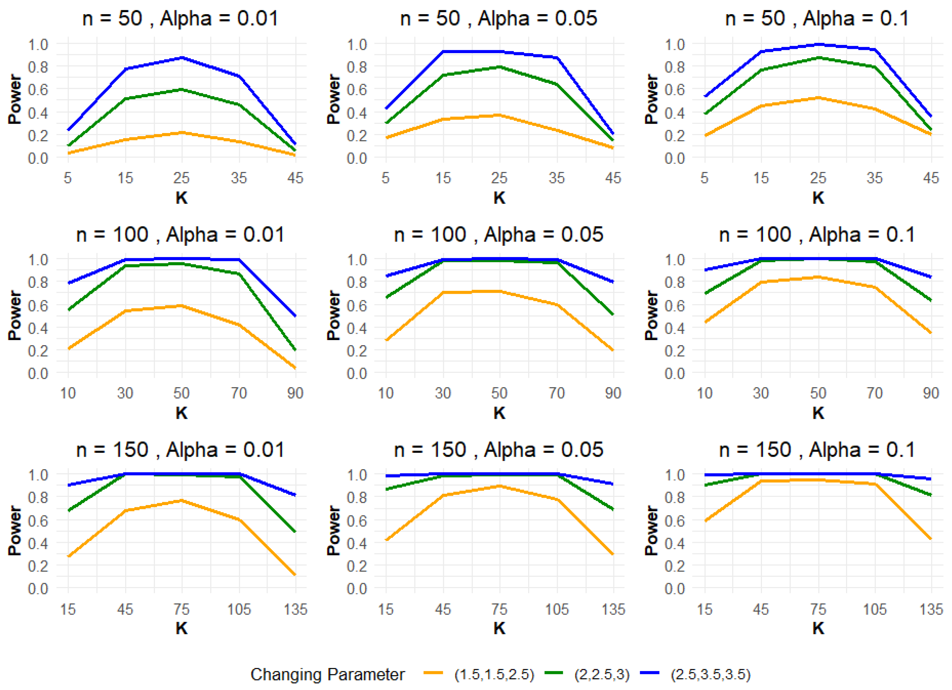
The sample sizes considered in the simulation study were n = 50, 100, and 150. The change-point location, denoted by K, was selected to represent structural changes occurring at different positions within the sample, approximately around ${\displaystyle \frac{1}{4}}$, ${\displaystyle \frac{1}{2}}$, and ${\displaystyle \frac{3}{4}}$ of the sample size n. Random samples from the EEL distribution were generated using the inverse transformation method based on the corresponding cumulative distribution function. Furthermore, the simulation results were obtained using N = 1000 Monte Carlo replications conducted under different significance levels. In this study, the empirical power is defined as the probability of rejecting the null hypothesis $H_0$ when a true change point exists in the generated data. The empirical power values were estimated as the proportion of Monte Carlo replications in which the proposed likelihood ratio test detected the presence of a structural change under the alternative hypothesis $H_1$. The empirical power in this simulation study reflects the ability of the test to detect the existence of a change point.

The corresponding empirical power values obtained from the simulation study are summarized in

Table 2. Power of the LRT for n = 50.

Changing Parameter	α	K = 5	K = 15	K = 25	K = 35	K = 45
(2.5, 1.5, 1.5)	0.10	0.190	0.450	0.520	0.425	0.200
	0.05	0.175	0.330	0.365	0.235	0.085
	0.01	0.040	0.155	0.215	0.135	0.020
(3, 2, 2.5)	0.10	0.380	0.770	0.875	0.790	0.230
	0.05	0.295	0.725	0.795	0.635	0.140
	0.01	0.095	0.510	0.595	0.455	0.055
(3.5, 2.5, 3.5)	0.10	0.535	0.930	0.995	0.945	0.350
	0.05	0.425	0.925	0.930	0.870	0.200
	0.01	0.230	0.775	0.870	0.710	0.105

,

Table 3. Power of the LRT for n = 100.

Changing Parameter	α	K = 10	K = 30	K = 50	K = 70	K = 90
(2.5, 1.5, 1.5)	0.10	0.445	0.795	0.835	0.745	0.340
	0.05	0.285	0.700	0.715	0.595	0.190
	0.01	0.205	0.545	0.590	0.415	0.040
(3, 2, 2.5)	0.10	0.695	0.980	1.000	0.970	0.630
	0.05	0.655	0.980	0.985	0.965	0.510
	0.01	0.550	0.940	0.960	0.865	0.190
(3.5, 2.5, 3.5)	0.10	0.905	1.000	1.000	1.000	0.835
	0.05	0.845	0.995	1.000	0.995	0.790
	0.01	0.785	0.995	1.000	0.995	0.490

and

Table 4. Power of the LRT for n = 150.

Changing Parameter	α	K = 15	K = 45	K = 75	K = 105	K = 135
(2.5, 1.5, 1.5)	0.10	0.585	0.935	0.945	0.915	0.425
	0.05	0.420	0.815	0.890	0.775	0.295
	0.01	0.270	0.680	0.770	0.595	0.110
(3, 2, 2.5)	0.10	0.905	1.000	1.000	1.000	0.810
	0.05	0.865	0.985	0.995	0.995	0.690
	0.01	0.675	1.000	0.995	0.975	0.490
(3.5, 2.5, 3.5)	0.10	0.990	1.000	1.000	1.000	0.955
	0.05	0.980	1.000	1.000	1.000	0.910
	0.01	0.905	1.000	1.000	1.000	0.810

, while the graphical representations of the power curves are illustrated in the accompanying Figure 1.

From Table 2, Table 3 and Table 4 and Figure 1, it can be observed that the empirical power of the LRT improves noticeably as the sample size increases and as the magnitude of the parameter changes becomes larger. In particular, for smaller sample sizes such as n = 50, the power values are relatively moderate, especially when the change point is located near the boundaries of the sample (i.e., for smaller or larger values of K). Nevertheless, the LRT exhibits higher power at central change point locations, such as K = 15 and K = 25, across all considered parameter configurations.

As the sample size increases to n = 100, the power of the LRT increases substantially for all parameter settings and significance levels. The results indicate that moderate changes in the parameters $(\theta ,\gamma ,\lambda )$ are detected with high accuracy, particularly when the change point occurs near the center of the sample. For larger parameter deviations, the LRT achieves power values close to 1 even for relatively early or late change point locations.

For the largest sample size (n = 150), the empirical power of the LRT approaches 1 in most scenarios, especially for larger parameter changes such as $(2.5,3.5,3.5)$. This demonstrates that the LRT becomes highly efficient in detecting change points when sufficient data are available and when the contrast between the pre- and post-change parameters is pronounced. The figures further illustrate that the power curves increase smoothly as a function of K, reaching their maximum values near the center of the sample and decreasing slightly toward the boundaries.

Overall, both the tabulated results and the graphical representations consistently indicate that larger sample sizes, stronger parameter shifts, and centrally located change points lead to higher detection power. These findings confirm the effectiveness of the LRT for change point detection in the EEL distribution and highlight its robustness under a wide range of experimental settings.

4. Application

In recent years, cryptocurrencies have received increasing attention due to their high volatility and susceptibility to structural changes driven by market dynamics, regulatory interventions, and technological innovations. Identifying such change points plays a crucial role in understanding market behaviors and enhancing decision-making in investment and risk management. In this paper, the proposed methodology is applied to two widely traded cryptocurrencies—namely, ETH and XRP —with the aim of detecting potential structural changes in their return series. The monthly return data for both cryptocurrencies were obtained from CoinMarketCap [36], covering the period from 1 January 2016 to 1 December 2023. To evaluate the suitability of the EEL distribution for the analyzed data, the Kolmogorov–Smirnov goodness-of-fit test was conducted. The obtained p-values were 0.7903 for ETH and 0.8916 for XRP, indicating that the cryptocurrency return data fit the EEL distribution well. These results support the adequacy of the EEL distribution for modeling cryptocurrency return series and demonstrate its ability to capture the underlying distributional characteristics of highly volatile financial data.

Since the cryptocurrency data displayed serial dependence, we converted prices to returns using the return series by Hsu [37]. Let $s_t$ denote the observed price index at time t. To construct a series of approximately independent observations, the return series $R_t$ is computed using the following transformation:

$$R_t={\displaystyle \frac{s_t-s_{t-1}}{s_{t-1}}},t=1,2,\dots ,n.$$

(5)

Prior to implementing the LRT procedure to detect possible change points in the real data, it is necessary to examine the independence assumption of the return series. To this end, the Portmanteau test, as proposed by Ngunkeng [38], is employed. The corresponding test statistic is given by

$$Q_o=n{\displaystyle \sum _{j=1}^o}{r}_j^2,$$

(6)

where $r_j$ denotes the autocorrelation coefficient at lag j, and o represents the number of lags included in the test. Under the null hypothesis of independence, the statistic $Q_o$ asymptotically follows a chi-square (${\chi }^2$) distribution with o degrees of freedom.

4.1. Ethereum Data

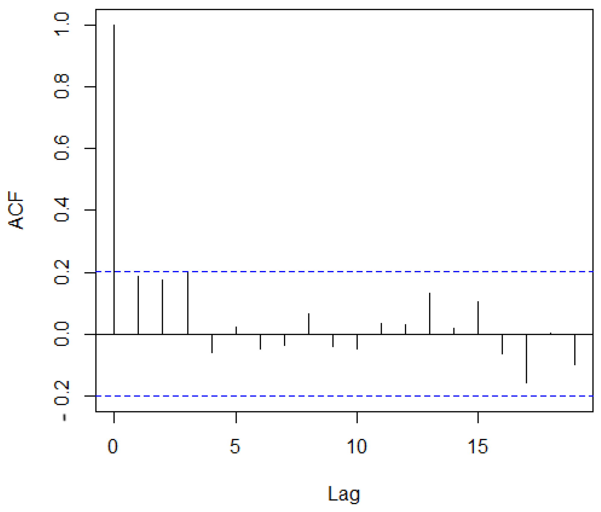
For the ETH dataset, the correlation test defined in Equation (6) was first applied to the original return series to assess potential temporal dependence. The test results indicated the presence of significant autocorrelation, necessitating a statistical transformation before further analysis. Consequently, the transformation in Equation (5) was applied to the data. As illustrated in Figure 2, the transformed ETH series appears to exhibit independence. To further confirm this observation, the Portmanteau test was conducted on the transformed dataset, yielding the following result:

$$Q_{12}=95{\displaystyle \sum _{j=1}^{12}}{r}_j^2=11.795<{\chi }_{0.95}^2\left(12\right)=21.026.$$

Therefore, we fail to reject $H_0$, indicating that the transformed data can be regarded as independent.

We applied the likelihood ratio test (LRT) combined with the binary segmentation procedure to detect all possible change points in the ETH series as follows.

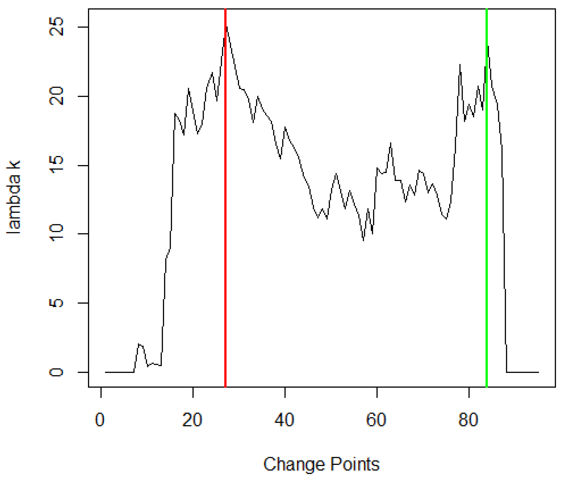
Step 1. Consider the sequence from positions 1 to 95. The test statistic is

$$Z_n^{\prime }=\underset{8\le k\le 87}{\max }{\Lambda }_k=25.2678>c_{0.05,95}=13.47423$$

and, therefore, the null hypothesis of no change is rejected. The first change point is detected at position k = 27.

Step 2. Using the binary segmentation procedure, the subsequences comprising positions 1 to 27 and 28 to 95 are examined separately. For the interval from positions 1 to 27, the test statistic does not exceed the corresponding critical value, indicating no additional change. For the interval from positions 28 to 95, the test statistic satisfies

$$Z_n^{\prime }=\underset{8\le k\le 60}{\max }{\Lambda }_k=17.94396>c_{0.05,68}=13.1588,$$

leading to the detection of a second change point at position k = 84.

Step 3. The remaining subsequences, comprising positions 28 to 84 and 85 to 95, are further tested. In both intervals, the test statistics are smaller than the corresponding critical values, indicating that no additional change points are present.

Therefore, we conclude that the ETH return series contains two change points located at positions 27 and 84. The final segmentation divides the data into three homogeneous segments—positions 1 to 27, 28 to 84, and 85 to 95—with no further structural changes detected within each segment. The results of the LRT-based detection procedure are presented in Figure 3.

Table 5. Estimated EEL parameters for the segments of the ETH dataset.

Segment	Observations	$\widehat{\mathit{\theta }}$	$\widehat{\mathit{\gamma }}$	$\widehat{\mathit{\lambda }}$
1	1–27	0.1223633	0.5403982	0.1690046
2	28–95	0.7129942	64.5573719	6.3988132
3	28–84	1.057424	354.962467	8.891616
4	85–95	0.08047526	3.77671711	1.94807204

presents the maximum likelihood estimates of the parameters θ, γ and λ for each segment in the ETH datasets. Two significant structural shifts were identified regarding the statistical behavior of the ETH return series. These change points correspond to periods during which the price dynamics of ETH underwent notable transitions. A summary of these shifts is provided below:

• Position 27 (April 2018): This change point aligns with a period in which ETH prices ranged approximately between USD 695 and 700. This phase marked the beginning of a major market correction following the sharp expansion of the cryptocurrency sector in 2017. From an analytical perspective, the detected change reflects a substantial shift in the distributional structure of the return series (see [36,39]).
• Position 84 (January 2023): The second change point corresponds to a recovery phase during which ETH prices rose to approximately USD 1645–2281 after the high volatility observed in 2022. Regarding the change point analysis, this transition indicates a shift toward a different return regime, characterized by comparatively greater stability and a gradual adjustment in the underlying statistical properties of the series (see [40,41]).

4.2. Ripple Data

For the XRP dataset, the same procedure as applied to the ETH data was performed. The correlation test defined in Equation (6) was first applied to the original XRP return series to assess potential temporal dependence. The results indicated the presence of autocorrelation, necessitating a statistical transformation prior to further analysis. Therefore, the transformation in Equation (5) was applied to the data.

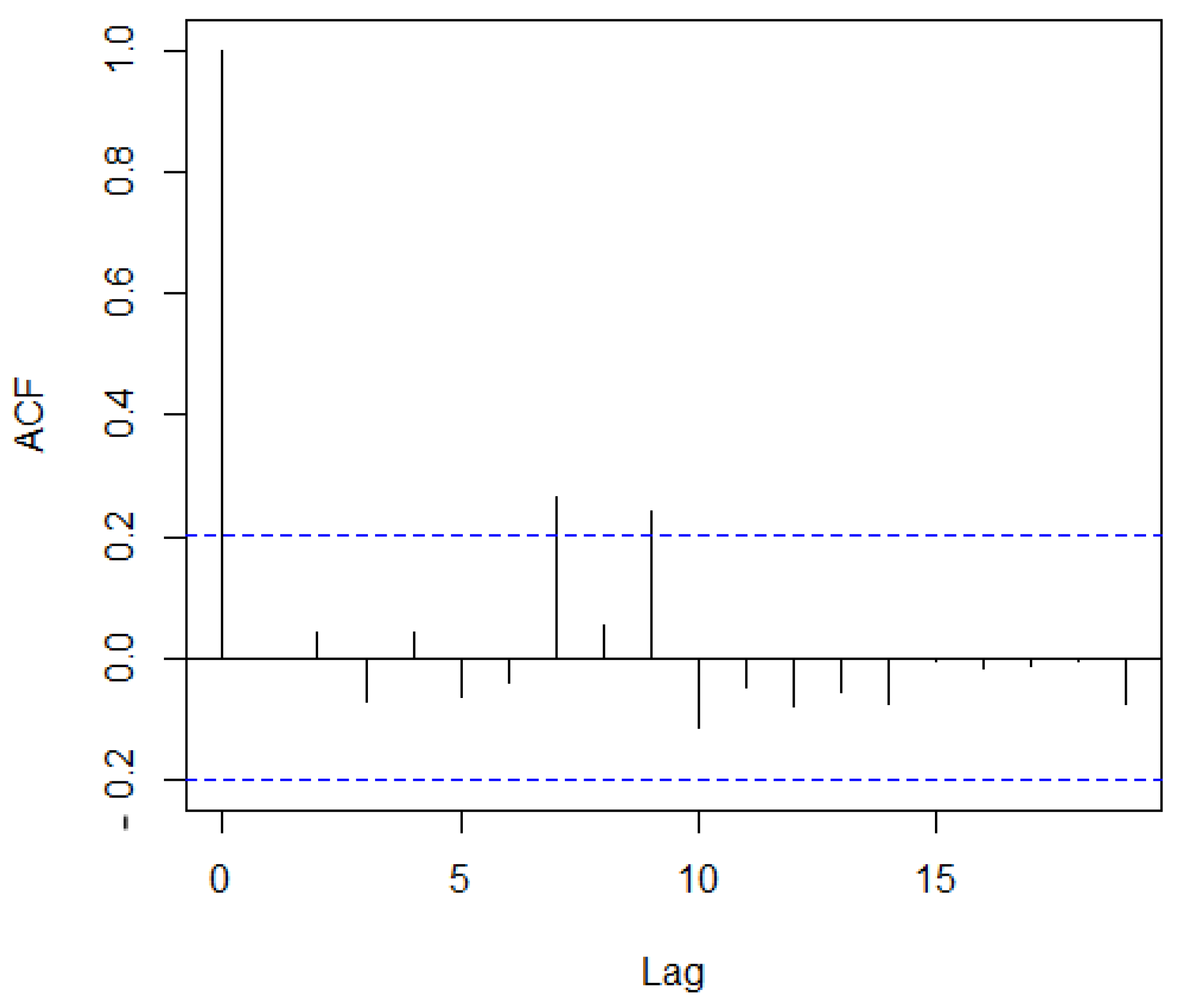
As illustrated in Figure 4, the transformed XRP series appears to exhibit independence. This observation is further supported by the Portmanteau test:

$$Q_{12}=95{\displaystyle \sum _{j=1}^{12}}{r}_j^2=16.023<{\chi }_{0.95}^2\left(12\right)=21.026.$$

Thus, we fail to reject $H_0$, confirming that the transformed XRP series is independent.

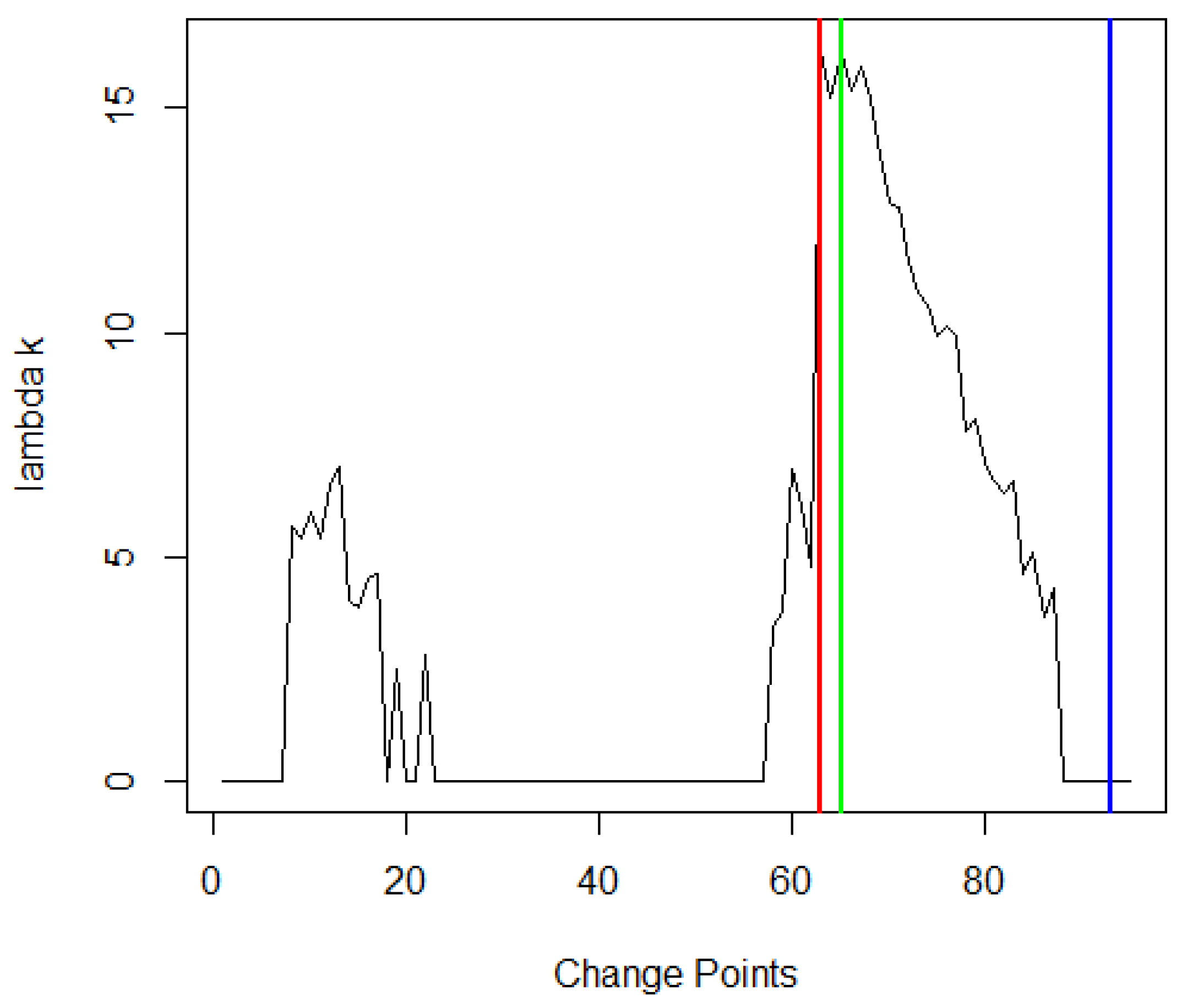
We applied the likelihood ratio test (LRT) combined with the binary segmentation procedure to detect all possible change points in the XRP series as follows.

Step 1. Consider the sequence from positions 1 to 95. The test statistic is

$$Z_n^{\prime }=\underset{8\le k\le 87}{\max }{\Lambda }_k=16.3191>c_{0.05,95}=13.47423$$

and, therefore, the null hypothesis of no change is rejected. The first change point is detected at position k = 63.

Step 2. Using the binary segmentation procedure, the subsequences comprising positions 1 to 63 and 64 to 95 are examined separately. For the interval from positions 1 to 63, the test statistic does not exceed the corresponding critical value, indicating that no change point is detected within this segment. For the interval from positions 64 to 95, the test statistic satisfies

$$Z_n^{\prime }=\underset{6\le k\le 26}{\max }{\Lambda }_k=15.55925>c_{0.05,32}=11.90221,$$

leading to the detection of a second change point at position k = 65.

Step 3. The remaining subsequence from positions 66 to 95 is further examined. For this interval, the test statistic is

$$Z_n^{\prime }=\underset{6\le k\le 24}{\max }{\Lambda }_k=14.68401>c_{0.05,30}=11.99086,$$

resulting in the detection of an additional change point at position k = 93.

Step 4. The remaining subsequence, comprising positions 66 to 93, are tested. In this case, the test statistic is smaller than the corresponding critical value, indicating that no additional change points are detected.

Therefore, we conclude that the XRP return series contains three change points, located at positions 63, 65, and 93. The final segmentation divides the data into four homogeneous segments—positions 1 to 63, 64 to 95, 66 to 95, and 66 to 93—with no further structural changes detected within any subinterval. The results of the LRT-based detection procedure are presented in Figure 5.

Table 6. Estimated EEL parameters for the segments of the XRP dataset.

Segment	Observations	$\widehat{\mathit{\theta }}$	$\widehat{\mathit{\gamma }}$	$\widehat{\mathit{\lambda }}$
1	1–63	0.02105735	0.12992173	0.01056084
2	64–95	0.9385198	570.1735487	9.9354950
3	66–95	0.9831037	999.2750623	10.5789393
4	66–93	0.8687541	346.0864148	9.0433643

presents the estimated EEL parameters θ, γ and λ for each segment identified by the binary segmentation method. Three notable structural changes were detected regarding the statistical behavior of the XRP return series. These change points mark periods in which the price dynamics of XRP underwent meaningful shifts. A summary of these changes is provided below.

• Position 63 (April 2021): This change point corresponds to a period in which XRP experienced a sharp upward movement, with prices rising by nearly 300% and approaching USD 2. This phase reflects a strong bullish momentum within the broader cryptocurrency market despite the ongoing legal dispute between Ripple Labs and the U.S. Securities and Exchange Commission (SEC). From an analytical perspective, this point signifies a substantial shift in the distributional structure of the return series (see [36,42]).
• Position 65 (June 2021): The second detected change point aligns with a noticeable price decline following the April peak, where XRP prices opened between USD 0.90 and 1.04 and closed around USD 0.70–0.71. This drop reflects a broader market correction after the rapid prior surge, combined with continued regulatory uncertainty related to the SEC lawsuit. From a change point analysis perspective, this period indicates a shift from a growth regime to a corrective regime, highlighting a structural change in the volatility and distributional behavior of the series (see [36,39]).
• Position 93 (October 2023): The third change point corresponds to a phase of moderate price recovery, with XRP opening around $0.52 and closing near $0.60. This period reflects renewed positive sentiment in the cryptocurrency market, supported by improved regulatory outlooks and increasing investor confidence. Analytically, this transition indicates a shift toward a more stable return regime, marking a structural change in the underlying price dynamics (see [40,43]).

5. Conclusions

In this paper, the LRT based on the EEL distribution was employed to detect change points in distribution parameters. The simulation results demonstrated that the LRT exhibits strong detection capability across a wide range of parameter configurations and sample sizes, with its empirical power improving as the magnitude of parameter changes and the sample size increase.

Furthermore, the application of the proposed LRT procedure to the monthly return series of ETH and XRP from January 2016 to December 2023 successfully identified several significant change points. These results not only revealed the number and locations of these change points but also provided valuable insights into potential structural shifts in the respective cryptocurrency markets. These findings highlight the effectiveness of the LRT as a reliable tool for change point detection in real-world financial time series and underscore its practical relevance for analyzing structural changes in volatile markets.

As part of future research, a comprehensive comparison between the proposed LRT approach and other well-known change-point detection methods, such as Bayesian approaches, the SIC, and the MIC, will be considered in order to further evaluate the relative performance and efficiency of the proposed method.