On Proportional Caputo-Hybrid Fractional Milne-Type Inequalities: Theory, Numerical Simulations, and Applications

Abstract

The goal of this study is to establish a new type of Milne-type inequality in the scope of fractional calculus with the aid of proportional Caputo-hybrid operators. We will focus on two different scopes of regularity, which contain functions whose first and second derivatives are convex, and functions whose first and second derivatives are Lipschitz continuous. We will base these estimates on a new integral identity of proportional Caputo-hybrid integrals. We will show that the smoothness of the derivative influences the shape of the bounds. Convexity will cause symmetry. Lipschitz continuity will contain bounds on the modulus of continuity. To show that our results are accurate and easy to obtain, we included a full numerical example with graphics and applications to quadrature error estimation.

1. Introduction

Numerical integration without a primitive can be daunting. However, numerical quadrature provides a solution to this problem by approximating the integral value through a weighted sum of the integral’s values at pre-chosen points (or nodes). The trapezoidal and Simpson’s rules offer a foundation for various modern numerical integration techniques. However, the aforementioned rules’ accuracy depends on the smoothness and shape of the function being integrated.

Numerous publications have focused on analyzing the precision of these methods, particularly when the integrated function does not possess a high degree of smoothness. Among the most successful functions to analyze smoothness is the convex function. Many researchers have successfully used various degrees of convexity (classical, strong, generalized) to form inequalities that bound the differences between the true value of an integral and its numerical approximation. For a pertinent review see [1].

Definition 1

([2]). A function $\mathcal{F}:\mathbf{I}\subset \mathbb{R}\to \mathbb{R}$ is deemed to be convex if

$$\mathcal{F}\left(\mu \mathfrak{v}+\left(1-\mu \right)\mathfrak{w}\right)\le \mu \mathcal{F}\left(\mathfrak{v}\right)+\left(1-\mu \right)\mathcal{F}\left(\mathfrak{w}\right)$$

is valid for all $\mathfrak{v},\mathfrak{w}\in \mathbf{I}$ and all $\mu \in [0,1]$.

One of the most interesting extensions of the convexity notion is s-convexity in the second sense, which is formulated as follows.

Definition 2

([3]). A nonnegative function $\mathcal{F}:\mathbf{I}\subset {\mathbb{R}}^{+}=\left[0,\infty \right)\to \mathbb{R}$ is deemed to be s-convex in the second sense for some fixed $s\in \left(0,1\right]$ if

$$\mathcal{F}(\mu \mathfrak{v}+(1-\mu )\mathfrak{w})\le {\mu }^s\mathcal{F}\left(\mathfrak{v}\right)+{(1-\mu )}^s\mathcal{F}\left(\mathfrak{w}\right)$$

is valid for all $\mathfrak{v},\mathfrak{w}\in \mathbf{I}$ and $\mu \in [0,1]$.

Among the increasingly studied rules is the Milne-type quadrature, which shares the three-point structure of Simpson’s formula but incorporates a distinct weighting that yields different error characteristics and is given by

$$\mathcal{M}\left({\mathfrak{d}}_1,{\mathfrak{d}}_2,\mathcal{F}\right)={\displaystyle \frac{1}{3}}\left(2\mathcal{F}\left({\mathfrak{d}}_1\right)-\mathcal{F}\left({\displaystyle \frac{{\mathfrak{d}}_1+{\mathfrak{d}}_2}{2}}\right)+2\mathcal{F}\left({\mathfrak{d}}_2\right)\right)\simeq {\displaystyle \frac{1}{{\mathfrak{d}}_2-{\mathfrak{d}}_1}}\underset{{\mathfrak{d}}_1}{\stackrel{{\mathfrak{d}}_2}{\int }}\mathcal{F}\left(\varpi \right)\mathrm{d}\varpi .$$

(1)

This rule has recently drawn attention due to its favorable convergence properties and its utility in constructing refined integral inequalities. Several authors have explored Milne-type inequalities under various convexity frameworks, including [4,5,6,7,8], where new estimates and generalizations have been established in both classical and extended settings.

Parallel to these developments, fractional calculus has provided a fertile ground for generalizing integral inequalities by introducing non-local operators that capture memory and hereditary effects. Fractional variants of Milne-type inequalities have been investigated using Riemann–Liouville fractional integrals [9,10,11,12], Ktugampola fractional integrals [13,14], and conformable fractional integrals [15,16], revealing deeper connections between numerical analysis and fractional modeling. For further results on Milne-type inequalities via different types of integral operators, we refer the reader to [17,18,19].

In [10], Budak and Hyder established the following Milne-type inequality for differentiable convex functions via Riemann–Liouville fractional integrals.

Theorem 1

([10]). Let $\mathcal{F}:[{\mathfrak{d}}_1,{\mathfrak{d}}_2]\to \mathbb{R}$ be a differentiable mapping on $({\mathfrak{d}}_1,{\mathfrak{d}}_2)$ such that $\mathcal{F}\in L_1\left([{\mathfrak{d}}_1,{\mathfrak{d}}_2]\right)$, where $L_1\left([{\mathfrak{d}}_1,{\mathfrak{d}}_2]\right)$ denotes the class of measurable functions that are absolutely integrable with ${\displaystyle {\int }_{{\sigma }_1}^{{\sigma }_2}\left|\mathcal{F}\left(t\right)\right|\mathrm{d}t<\infty }$. If $\left|{\mathcal{F}}^{\prime }\right|$ is convex on $[{\mathfrak{d}}_1,{\mathfrak{d}}_2]$. Then, we have

$$\begin{array}{cc}\hfill & \left|{\displaystyle \frac{1}{3}}\left(2\mathcal{F}\left({\mathfrak{d}}_1\right)-\mathcal{F}\left({\displaystyle \frac{{\mathfrak{d}}_1+{\mathfrak{d}}_2}{2}}\right)+2\mathcal{F}\left({\mathfrak{d}}_2\right)\right)-{\displaystyle \frac{\Gamma \left(\varrho +1\right)}{2{\left({\mathfrak{d}}_2-{\mathfrak{d}}_1\right)}^{\varrho }}}\left({\mathbf{J}}_{{\mathfrak{d}}_1^{+}}^{\varrho }\mathcal{F}\left({\mathfrak{d}}_2\right)+{\mathbf{J}}_{{\mathfrak{d}}_2^{-}}^{\varrho }\mathcal{F}\left({\mathfrak{d}}_1\right)\right)\right|\hfill \\ \hfill \le & {\displaystyle \frac{{\mathfrak{d}}_2-{\mathfrak{d}}_1}{2}}\left({\mathcal{B}}_1\left(\varrho \right)+{\mathcal{B}}_2\left(\varrho \right)\right)\left(\left|{\mathcal{F}}^{\prime }\left({\mathfrak{d}}_1\right)\right|+\left|{\mathcal{F}}^{\prime }\left({\mathfrak{d}}_2\right)\right|\right),\hfill \end{array}$$

where ${\mathbf{J}}_{{\mathfrak{d}}_1^{+}}^{\varrho }$ and ${\mathbf{J}}_{{\mathfrak{d}}_2^{-}}^{\varrho }$ denote the left- and right-hand-sided Riemann–Liouville fractional integrals of order ϱ expressed as

$${\mathbf{J}}_{{\mathfrak{d}}_1^{+}}^{\varrho }\mathcal{F}\left(x\right)={\displaystyle \frac{1}{\Gamma \left(\varrho \right)}}{\int }_{{\mathfrak{d}}_1}^x{\left(x-\mu \right)}^{\varrho -1}\mathcal{F}\left(\mu \right)\mathrm{d}\mu ,x>{\mathfrak{d}}_1,$$

$${\mathbf{J}}_{{\mathfrak{d}}_2^{-}}^{\varrho }\mathcal{F}\left(x\right)={\displaystyle \frac{1}{\Gamma \left(\varrho \right)}}{\int }_x^{{\mathfrak{d}}_2}{\left(\mu -x\right)}^{\varrho -1}\mathcal{F}\left(\mu \right)\mathrm{d}\mu ,x<{\mathfrak{d}}_2,$$

where $\Gamma \left(\varrho \right)$ denotes the Euler Gamma function $\Gamma \left(\varrho \right)=\underset{0}{\stackrel{1}{\int }}{\mu }^{\varrho -1}{e}^{-\mu }\mathrm{d}\mu$, and ${\mathcal{B}}_1\left(\varrho \right)$ and ${\mathcal{B}}_2\left(\varrho \right)$ are given by

$${\mathcal{B}}_1\left(\varrho \right)=\left\{\begin{array}{ccc}{\displaystyle \frac{2\varrho }{\varrho +1}}{\left({\displaystyle \frac{2}{3}}\right)}^{\frac{1}{\varrho }+1}+{\displaystyle \frac{1}{2^{\varrho +1}\left(\varrho +1\right)}}-{\displaystyle \frac{1}{3}}\hfill & for& 0<\varrho \le {\displaystyle \frac{\ln 3-\ln 2}{\ln 2}}\\ {\displaystyle \frac{1}{3}}-{\displaystyle \frac{1}{2^{\varrho +1}\left(\varrho +1\right)}}\hfill & for& \varrho >{\displaystyle \frac{\ln 3-\ln 2}{\ln 2}}\end{array}\right.$$

and

$${\mathcal{B}}_2\left(\varrho \right)=\left\{\begin{array}{ccc}{\displaystyle \frac{1}{\varrho +1}}-{\displaystyle \frac{1}{2^{\varrho +1}\left(\varrho +1\right)}}-\frac{1}{6}\hfill & for& 0<\varrho \le {\displaystyle \frac{\ln 3}{\ln 2}}\\ {\displaystyle \frac{2\varrho }{\varrho +1}}{\left({\displaystyle \frac{1}{3}}\right)}^{\frac{1}{\varrho }+1}+{\displaystyle \frac{1}{2^{\varrho +1}\left(\varrho +1\right)}}+{\displaystyle \frac{1}{\varrho +1}}-{\displaystyle \frac{1}{2}}\hfill & for& \varrho >{\displaystyle \frac{\ln 3}{\ln 2}},\end{array}\right.$$

respectively.

In [20], Baleanu et al. introduced a novel fractional operator based on a generalized proportional derivative. This operator admits an equivalent representation as a Riemann–Liouville integral applied to the proportional derivative. Moreover, under certain key specializations, it reduces to a linear combination of a Riemann–Liouville fractional integral and a Caputo fractional derivative.

Definition 3

([20]). Let $\mathcal{F}:\mathbf{I}\subset {\mathbb{R}}^{+}\to \mathbb{R}$ be a differentiable function on ${\mathbf{I}}^{\circ }$ (the interior of the interval $\mathbf{I}$), and $\mathcal{F},{\mathcal{F}}^{\prime }\in L\left(\mathbf{I}\right)$. The proportional Caputo-hybrid operator of order ϱ is defined as

$${}_0\mathcal{D}_{\varpi }^{\varrho }\mathcal{F}\left(\varpi \right)={\displaystyle \frac{1}{\Gamma \left(1-\varrho \right)}}\stackrel{\varpi }{\underset{0}{\int }}\left({\mathcal{K}}_1\left(\varrho ,\mathfrak{v}\right)\mathcal{F}\left(\mathfrak{v}\right)+{\mathcal{K}}_0\left(\varrho ,\mathfrak{v}\right){\mathcal{F}}^{\prime }\left(\mathfrak{v}\right)\right){\left(\varpi -\mathfrak{v}\right)}^{-\varrho }\mathrm{d}\mathfrak{v},$$

where $\varrho \in \left(0,1\right)$ and ${\mathcal{K}}_0$ and ${\mathcal{K}}_1$ are two variable functions $(0,1)\times \mathbf{I}\to \mathbb{R}$ and satisfy

$$\underset{\varrho \to 0^{+}}{\lim }{\mathcal{K}}_0(\varrho ,\mathfrak{v})=0;\underset{\varrho \to 1^{-}}{\lim }{\mathcal{K}}_0(\varrho ,\mathfrak{v})=1;with{\mathcal{K}}_0(\varrho ,\mathfrak{v})\ne 0,$$

and

$$\underset{\varrho \to 0^{+}}{\lim }{\mathcal{K}}_1(\varrho ,\mathfrak{v})=0;\underset{\varrho \to 1^{-}}{\lim }{\mathcal{K}}_1(\varrho ,\mathfrak{v})=0;with{\mathcal{K}}_1(\varrho ,\mathfrak{v})\ne 0.$$

Remark 1

([20]). By assigning the boundary values $\varrho =0$ and $\varrho =1$, we deduce the following distinct forms:

$$\underset{\varrho \to 0}{\lim }{}_0\mathcal{D}_{\varpi }^{\varrho }\mathcal{F}\left(\varpi \right)=\underset{0}{\stackrel{\varpi }{\int }}\mathcal{F}\left(\mathfrak{v}\right)\mathrm{d}\mathfrak{v},$$

and

$$\underset{\varrho \to 1}{\lim }{}_0\mathcal{D}_{\varpi }^{\varrho }\mathcal{F}\left(\varpi \right)={\mathcal{F}}^{\prime }\left(\varpi \right).$$

Subsequently, by using specific functions ${\mathcal{K}}_0$ and ${\mathcal{K}}_1$, Sarikaya presented the following definition of proportional Caputo-hybrid fractional operators:

Definition 4

([21]). Let $\mathcal{F}:\mathbf{I}\subset {\mathbb{R}}^{+}\to \mathbb{R}$ be a differentiable function on ${\mathbf{I}}^{\circ }$ (the interior of the interval $\mathbf{I}$), and $\mathcal{F},{\mathcal{F}}^{\prime }\in L_1\left(\mathbf{I}\right)$. The left- and right-sided proportional Caputo-hybrid operators of order ϱ are defined, respectively, as follows:

$${\mathcal{D}}_{{\mathfrak{d}}_1^{+}}^{\varrho }\mathcal{F}\left({\mathfrak{d}}_2\right)={\displaystyle \frac{1}{\Gamma \left(1-\varrho \right)}}\stackrel{{\mathfrak{d}}_2}{\underset{{\mathfrak{d}}_1}{\int }}\left({\mathcal{K}}_1\left(\varrho ,{\mathfrak{d}}_2-\mathfrak{v}\right)\mathcal{F}\left(\mathfrak{v}\right)+{\mathcal{K}}_0\left(\varrho ,{\mathfrak{d}}_2-\mathfrak{v}\right){\mathcal{F}}^{\prime }\left(\mathfrak{v}\right)\right){\left({\mathfrak{d}}_2-\mathfrak{v}\right)}^{-\varrho }\mathrm{d}\mathfrak{v},$$

and

$${\mathcal{D}}_{{\mathfrak{d}}_2^{-}}^{\varrho }\mathcal{F}\left({\mathfrak{d}}_1\right)={\displaystyle \frac{1}{\Gamma \left(1-\varrho \right)}}\stackrel{{\mathfrak{d}}_2}{\underset{{\mathfrak{d}}_1}{\int }}\left({\mathcal{K}}_1\left(\varrho ,\mathfrak{v}-{\mathfrak{d}}_1\right)\mathcal{F}\left(\mathfrak{v}\right)+{\mathcal{K}}_0\left(\varrho ,\mathfrak{v}-{\mathfrak{d}}_1\right){\mathcal{F}}^{\prime }\left(\mathfrak{v}\right)\right){\left(\mathfrak{v}-{\mathfrak{d}}_1\right)}^{-\varrho }\mathrm{d}\mathfrak{v},$$

where $\varrho \in \left(0,1\right)$ and ${\mathcal{K}}_0\left(\varrho ,\mathfrak{v}\right)={(1-\varrho )}^2{\mathfrak{v}}^{1-\varrho }$ and ${\mathcal{K}}_1\left(\varrho ,\mathfrak{v}\right)={\varrho }^2{\mathfrak{v}}^{\varrho }$.

We emphasize that, consistent with the observations in Remark 1, choosing the values $\varrho =0$ and $\varrho =1$ results in

$$\underset{\varrho \to 0}{\lim }{\mathcal{D}}_{{\mathfrak{d}}_1^{+}}^{\varrho }\mathcal{F}\left({\mathfrak{d}}_2\right)=\underset{\varrho \to 1}{\lim }{\mathcal{D}}_{{\mathfrak{d}}_2^{-}}^{\varrho }\mathcal{F}\left({\mathfrak{d}}_1\right)=\underset{{\mathfrak{d}}_1}{\stackrel{{\mathfrak{d}}_2}{\int }}\mathcal{F}\left(\mathfrak{v}\right)\mathrm{d}\mathfrak{v},$$

and

$$\underset{\varrho \to 1}{\lim }{\mathcal{D}}_{{\mathfrak{d}}_1^{+}}^{\varrho }\mathcal{F}\left({\mathfrak{d}}_2\right)={\mathcal{F}}^{\prime }\left({\mathfrak{d}}_2\right),\underset{\varrho \to 0}{\lim }{\mathcal{D}}_{{\mathfrak{d}}_2^{-}}^{\varrho }\mathcal{F}\left({\mathfrak{d}}_1\right)={\mathcal{F}}^{\prime }\left({\mathfrak{d}}_1\right).$$

For the limiting case $\varrho \to 1$, the convergence of the singular terms to the Dirac delta distribution $\delta ({\mathfrak{d}}_2-\mathfrak{v})$ and $\delta (\mathfrak{v}-{\mathfrak{d}}_1)$ act as an approximation to the identity, which, coupled with the vanishing kernel ${\mathcal{K}}_1$, directly extracts the first derivative ${\mathcal{F}}^{\prime }\left({\mathfrak{d}}_2\right)$ and ${\mathcal{F}}^{\prime }\left({\mathfrak{d}}_1\right)$ from the integral.

In the same work [21], Sarikaya presented the Hermite–Hadamard and trapezium-type inequalities using convexity via proportional Caputo-hybrid operators. Furthermore, via the same operators and for functions whose first-order and second-order derivatives are convex, Sarikaya [22] gave the Simpson-type inequality. In [23], Demir and Tunç established Newton-type inequalities for twice differentiable functions via proportional Caputo-hybrid operators. More recently, Mehtab et al. [24] provided corrected Euler–Maclaurin-type inequalities via convexity, along with computational analysis and applications.

In [25], Demir established the following Milne-type inequalities for functions whose first-order and second-order derivatives are convex and $\varrho \in (0,1)$:

$$\begin{array}{cc}\hfill & |{\displaystyle \frac{{\varrho }^2{\left({\mathfrak{d}}_2-{\mathfrak{d}}_1\right)}^{\varrho }}{2^{\varrho }}}\mathcal{M}\left({\mathfrak{d}}_1,{\mathfrak{d}}_2,\mathcal{F}\right)+{\displaystyle \frac{\left(1-\varrho \right){\left({\mathfrak{d}}_2-{\mathfrak{d}}_1\right)}^{1-\varrho }}{2^{2-\varrho }}}\mathcal{M}\left({\mathfrak{d}}_1,{\mathfrak{d}}_2,{\mathcal{F}}^{\prime }\right)\hfill \\ \hfill & -{\displaystyle \frac{\Gamma \left(1-\varrho \right)}{2^{\varrho }{\left({\mathfrak{d}}_2-{\mathfrak{d}}_1\right)}^{1-\varrho }}}\left({\mathcal{D}}_{{\left(\frac{{\mathfrak{d}}_1+{\mathfrak{d}}_2}{2}\right)}^{-}}^{\varrho }\mathcal{F}\left({\mathfrak{d}}_1\right)+{\mathcal{D}}_{{\left(\frac{{\mathfrak{d}}_1+{\mathfrak{d}}_2}{2}\right)}^{+}}^{\varrho }\mathcal{F}\left({\mathfrak{d}}_2\right)\right)|\hfill \\ \hfill \le & {\displaystyle \frac{5{\varrho }^2{\left({\mathfrak{d}}_2-{\mathfrak{d}}_1\right)}^{\varrho +1}}{3\times 2^{\varrho +3}}}\left(\left|{\mathcal{F}}^{\prime }\left({\mathfrak{d}}_1\right)\right|+\left|{\mathcal{F}}^{\prime }\left({\mathfrak{d}}_2\right)\right|\right)\hfill \\ \hfill & +\left(1-\varrho \right){\left({\mathfrak{d}}_2-{\mathfrak{d}}_1\right)}^{2-\varrho }\left({\displaystyle \frac{2^{\varrho -3}\left(11-8\varrho \right)}{6(3-2\varrho )}}\right)\left(\left|{\mathcal{F}}^{″}\left({\mathfrak{d}}_1\right)\right|+\left|{\mathcal{F}}^{″}\left({\mathfrak{d}}_2\right)\right|\right),\hfill \end{array}$$

where $\mathcal{M}\left({\mathfrak{d}}_1,{\mathfrak{d}}_2,\mathcal{F}\right)$ is defined as in (1).

In an additional publication [26], the author derived inequalities of the Milne type for several categories of functions, such as bounded mappings, Lipschitz continuous functions, and those of bounded variation.

In this work, we establish new variants of Milne-type inequalities via proportional Caputo-hybrid operators, leveraging the convexity and Lipschitz continuity of ${\mathcal{F}}^{\prime }$ and ${\mathcal{F}}^{″}$. To this end, we begin by introducing a novel integral identity involving proportional Caputo-hybrid integrals in Section 2. Building on this identity, we derive numerous Milne-type inequalities in Section 3 for functions whose first-order and second-order derivatives are either convex or Lipschitz continuous. To validate the sharpness and highlight the practical implications of our results, in Section 4 we provide a numerical example with graphical illustration, along with some applications. The study concludes with a summary of the main findings in Section 5.

2. Proportional Caputo-Hybrid Identity

To lay the analytical groundwork for our inequalities, we first establish a new integral identity involving proportional Caputo-hybrid fractional integrals.

Lemma 1.

Let $\mathcal{F}:\mathbf{I}\to \mathbb{R}$ be a twice differentiable function on ${\mathbf{I}}^{\circ }$, where ${\mathfrak{d}}_1,{\mathfrak{d}}_2\in {\mathbf{I}}^{\circ }$ satisfying ${\mathfrak{d}}_1<{\mathfrak{d}}_2$ and let $\mathcal{F},{\mathcal{F}}^{\prime },{\mathcal{F}}^{″}\in L_1\left[{\mathfrak{d}}_1,{\mathfrak{d}}_2\right]$. Then, for $\varrho \in (0,1)$, the following equality

$$\begin{array}{cc}\hfill & {\varrho }^2{\left({\mathfrak{d}}_2-{\mathfrak{d}}_1\right)}^{\varrho }\mathcal{M}\left({\mathfrak{d}}_1,{\mathfrak{d}}_2,\mathcal{F}\right)+{\displaystyle \frac{1-\varrho }{2{\left({\mathfrak{d}}_2-{\mathfrak{d}}_1\right)}^{\varrho -1}}}\mathcal{M}\left({\mathfrak{d}}_1,{\mathfrak{d}}_2,{\mathcal{F}}^{\prime }\right)-{\displaystyle \frac{\Gamma \left(1-\varrho \right)}{2{\left({\mathfrak{d}}_2-{\mathfrak{d}}_1\right)}^{1-\varrho }}}\left({\mathcal{D}}_{{\mathfrak{d}}_2^{-}}^{\varrho }\mathcal{F}\left({\mathfrak{d}}_1\right)+{\mathcal{D}}_{{\mathfrak{d}}_1^{+}}^{\varrho }\mathcal{F}\left({\mathfrak{d}}_2\right)\right)\hfill \\ \hfill =& {\varrho }^2{\left({\mathfrak{d}}_2-{\mathfrak{d}}_1\right)}^{\varrho }\underset{0}{\stackrel{\frac{1}{2}}{\int }}\left(\mu -{\displaystyle \frac{2}{3}}\right)\left({\mathcal{F}}^{\prime }\left(\left(1-\mu \right){\mathfrak{d}}_1+\mu {\mathfrak{d}}_2\right)-{\mathcal{F}}^{\prime }\left(\mu {\mathfrak{d}}_1+\left(1-\mu \right){\mathfrak{d}}_2\right)\right)\mathrm{d}\mu \hfill \\ \hfill & +{\displaystyle \frac{\left(1-\varrho \right){\left({\mathfrak{d}}_2-{\mathfrak{d}}_1\right)}^{2-\varrho }}{4}}\left(\underset{0}{\stackrel{\frac{1}{2}}{\int }}\left({\mu }^{2-2\varrho }-{\displaystyle \frac{2}{3}}\right)\left({\mathcal{F}}^{″}\left(\left(1-\mu \right){\mathfrak{d}}_1+\mu {\mathfrak{d}}_2\right)-{\mathcal{F}}^{″}\left(\mu {\mathfrak{d}}_1+\left(1-\mu \right){\mathfrak{d}}_2\right)\right)\mathrm{d}\mu \right.\hfill \\ \hfill & +\left.\underset{\frac{1}{2}}{\stackrel{1}{\int }}\left({\mu }^{2-2\varrho }-{\displaystyle \frac{1}{3}}\right)\left({\mathcal{F}}^{″}\left(\left(1-\mu \right){\mathfrak{d}}_1+\mu {\mathfrak{d}}_2\right)-{\mathcal{F}}^{″}\left(\mu {\mathfrak{d}}_1+\left(1-\mu \right){\mathfrak{d}}_2\right)\right)\mathrm{d}\mu \right),\hfill \end{array}$$

holds, where $\mathcal{M}\left({\mathfrak{d}}_1,{\mathfrak{d}}_2,\mathcal{F}\right)$ is defined as in (1), and $\Gamma (·)$ is referred to as the well-known Γ-function.

Proof. 

Let

$${\mathcal{I}}_1=\underset{0}{\stackrel{\frac{1}{2}}{\int }}\left(\mu -{\displaystyle \frac{2}{3}}\right)\left({\mathcal{F}}^{\prime }\left(\left(1-\mu \right){\mathfrak{d}}_1+\mu {\mathfrak{d}}_2\right)-{\mathcal{F}}^{\prime }\left(\mu {\mathfrak{d}}_1+\left(1-\mu \right){\mathfrak{d}}_2\right)\right)\mathrm{d}\mu ,$$

$${\mathcal{I}}_2=\underset{0}{\stackrel{\frac{1}{2}}{\int }}\left({\mu }^{2-2\varrho }-{\displaystyle \frac{2}{3}}\right)\left({\mathcal{F}}^{″}\left(\left(1-\mu \right){\mathfrak{d}}_1+\mu {\mathfrak{d}}_2\right)-{\mathcal{F}}^{″}\left(\mu {\mathfrak{d}}_1+\left(1-\mu \right){\mathfrak{d}}_2\right)\right)\mathrm{d}\mu$$

and

$${\mathcal{I}}_3=\underset{\frac{1}{2}}{\stackrel{1}{\int }}\left({\mu }^{2-2\varrho }-{\displaystyle \frac{1}{3}}\right)\left({\mathcal{F}}^{″}\left(\left(1-\mu \right){\mathfrak{d}}_1+\mu {\mathfrak{d}}_2\right)-{\mathcal{F}}^{″}\left(\mu {\mathfrak{d}}_1+\left(1-\mu \right){\mathfrak{d}}_2\right)\right)\mathrm{d}\mu .$$

Using the integration by parts, ${\mathcal{I}}_1$ gives

$$\begin{array}{cc}\hfill {\mathcal{I}}_1=& {\left.{\displaystyle \frac{1}{{\mathfrak{d}}_2-{\mathfrak{d}}_1}}\left(\mu -{\displaystyle \frac{2}{3}}\right)\left(\mathcal{F}\left(\left(1-\mu \right){\mathfrak{d}}_1+\mu {\mathfrak{d}}_2\right)+\mathcal{F}\left(\mu {\mathfrak{d}}_1+\left(1-\mu \right){\mathfrak{d}}_2\right)\right)\right|}_0^{\frac{1}{2}}\hfill \\ \hfill & -{\displaystyle \frac{1}{{\mathfrak{d}}_2-{\mathfrak{d}}_1}}\underset{0}{\stackrel{\frac{1}{2}}{\int }}\left(\mathcal{F}\left(\left(1-\mu \right){\mathfrak{d}}_1+\mu {\mathfrak{d}}_2\right)+\mathcal{F}\left(\mu {\mathfrak{d}}_1+\left(1-\mu \right){\mathfrak{d}}_2\right)\right)\mathrm{d}\mu \hfill \\ \hfill =& {\displaystyle \frac{1}{{\mathfrak{d}}_2-{\mathfrak{d}}_1}}\left[{\displaystyle \frac{2}{3}}\left(\mathcal{F}\left({\mathfrak{d}}_1\right)+\mathcal{F}\left({\mathfrak{d}}_2\right)\right)-{\displaystyle \frac{1}{3}}\mathcal{F}\left({\displaystyle \frac{{\mathfrak{d}}_1+{\mathfrak{d}}_2}{2}}\right)\right]\hfill \\ \hfill & -{\displaystyle \frac{1}{{\mathfrak{d}}_2-{\mathfrak{d}}_1}}\underset{0}{\stackrel{\frac{1}{2}}{\int }}\left(\mathcal{F}\left(\left(1-\mu \right){\mathfrak{d}}_1+\mu {\mathfrak{d}}_2\right)+\mathcal{F}\left(\mu {\mathfrak{d}}_1+\left(1-\mu \right){\mathfrak{d}}_2\right)\right)\mathrm{d}\mu .\hfill \end{array}$$

(2)

Likewise, we get

$$\begin{array}{cc}\hfill {\mathcal{I}}_2=& {\left.{\displaystyle \frac{1}{{\mathfrak{d}}_2-{\mathfrak{d}}_1}}\left({\mu }^{2-2\varrho }-{\displaystyle \frac{2}{3}}\right)\left({\mathcal{F}}^{\prime }\left(\left(1-\mu \right){\mathfrak{d}}_1+\mu {\mathfrak{d}}_2\right)+{\mathcal{F}}^{\prime }\left(\mu {\mathfrak{d}}_1+\left(1-\mu \right){\mathfrak{d}}_2\right)\right)\right|}_0^{\frac{1}{2}}\hfill \\ \hfill & -{\displaystyle \frac{2-2\varrho }{{\mathfrak{d}}_2-{\mathfrak{d}}_1}}\underset{0}{\stackrel{\frac{1}{2}}{\int }}{\mu }^{1-2\varrho }\left({\mathcal{F}}^{\prime }\left(\left(1-\mu \right){\mathfrak{d}}_1+\mu {\mathfrak{d}}_2\right)+{\mathcal{F}}^{\prime }\left(\mu {\mathfrak{d}}_1+\left(1-\mu \right){\mathfrak{d}}_2\right)\right)\mathrm{d}\mu \hfill \\ \hfill =& {\displaystyle \frac{1}{{\mathfrak{d}}_2-{\mathfrak{d}}_1}}\left[2\left({\left({\displaystyle \frac{1}{2}}\right)}^{2-2\varrho }-{\displaystyle \frac{2}{3}}\right){\mathcal{F}}^{\prime }\left({\displaystyle \frac{{\mathfrak{d}}_1+{\mathfrak{d}}_2}{2}}\right)+{\displaystyle \frac{2}{3}}\left({\mathcal{F}}^{\prime }\left({\mathfrak{d}}_1\right)+{\mathcal{F}}^{\prime }\left({\mathfrak{d}}_2\right)\right)\right]\hfill \\ \hfill & -{\displaystyle \frac{2-2\varrho }{{\mathfrak{d}}_2-{\mathfrak{d}}_1}}\underset{0}{\stackrel{\frac{1}{2}}{\int }}{\mu }^{1-2\varrho }\left({\mathcal{F}}^{\prime }\left(\left(1-\mu \right){\mathfrak{d}}_1+\mu {\mathfrak{d}}_2\right)+{\mathcal{F}}^{\prime }\left(\mu {\mathfrak{d}}_1+\left(1-\mu \right){\mathfrak{d}}_2\right)\right)\mathrm{d}\mu ,\hfill \end{array}$$

(3)

and

$$\begin{array}{cc}\hfill {\mathcal{I}}_3=& {\left.{\displaystyle \frac{1}{{\mathfrak{d}}_2-{\mathfrak{d}}_1}}\left({\mu }^{2-2\varrho }-{\displaystyle \frac{1}{3}}\right)\left({\mathcal{F}}^{\prime }\left(\left(1-\mu \right){\mathfrak{d}}_1+\mu {\mathfrak{d}}_2\right)+{\mathcal{F}}^{\prime }\left(\mu {\mathfrak{d}}_1+\left(1-\mu \right){\mathfrak{d}}_2\right)\right)\right|}_{\frac{1}{2}}^1\hfill \\ \hfill & -{\displaystyle \frac{2-2\varrho }{{\mathfrak{d}}_2-{\mathfrak{d}}_1}}\underset{\frac{1}{2}}{\stackrel{1}{\int }}{\mu }^{1-2\varrho }\left({\mathcal{F}}^{\prime }\left(\left(1-\mu \right){\mathfrak{d}}_1+\mu {\mathfrak{d}}_2\right)+{\mathcal{F}}^{\prime }\left(\mu {\mathfrak{d}}_1+\left(1-\mu \right){\mathfrak{d}}_2\right)\right)\mathrm{d}\mu \hfill \\ \hfill =& {\displaystyle \frac{1}{{\mathfrak{d}}_2-{\mathfrak{d}}_1}}\left[{\displaystyle \frac{2}{3}}\left({\mathcal{F}}^{\prime }\left({\mathfrak{d}}_1\right)+{\mathcal{F}}^{\prime }\left({\mathfrak{d}}_2\right)\right)-\left({\left({\displaystyle \frac{1}{2}}\right)}^{2-2\varrho }-{\displaystyle \frac{1}{3}}\right){\mathcal{F}}^{\prime }\left({\displaystyle \frac{{\mathfrak{d}}_1+{\mathfrak{d}}_2}{2}}\right)\right]\hfill \\ \hfill & -{\displaystyle \frac{2-2\varrho }{{\mathfrak{d}}_2-{\mathfrak{d}}_1}}\underset{{\displaystyle \frac{1}{2}}}{\stackrel{1}{\int }}{\mu }^{1-2\varrho }\left({\mathcal{F}}^{\prime }\left(\left(1-\mu \right){\mathfrak{d}}_1+\mu {\mathfrak{d}}_2\right)+{\mathcal{F}}^{\prime }\left(\mu {\mathfrak{d}}_1+\left(1-\mu \right){\mathfrak{d}}_2\right)\right)\mathrm{d}\mu .\hfill \end{array}$$

(4)

By performing a change of variables, (2) yields

$$\begin{array}{cc}\hfill {\mathcal{I}}_1=& {\displaystyle \frac{1}{{\mathfrak{d}}_2-{\mathfrak{d}}_1}}\left({\displaystyle \frac{2\mathcal{F}\left({\mathfrak{d}}_1\right)-\mathcal{F}\left(\frac{{\mathfrak{d}}_1+{\mathfrak{d}}_2}{2}\right)+2\mathcal{F}\left({\mathfrak{d}}_2\right)}{3}}\right)-{\displaystyle \frac{1}{{\mathfrak{d}}_2-{\mathfrak{d}}_1}}\underset{0}{\stackrel{1}{\int }}\mathcal{F}\left(\left(1-\mu \right){\mathfrak{d}}_1+\mu {\mathfrak{d}}_2\right)\mathrm{d}\mu \hfill \\ \hfill =& {\displaystyle \frac{1}{{\mathfrak{d}}_2-{\mathfrak{d}}_1}}\left({\displaystyle \frac{2\mathcal{F}\left({\mathfrak{d}}_1\right)-\mathcal{F}\left(\frac{{\mathfrak{d}}_1+{\mathfrak{d}}_2}{2}\right)+2\mathcal{F}\left({\mathfrak{d}}_2\right)}{3}}\right)-{\displaystyle \frac{1}{{\left({\mathfrak{d}}_2-{\mathfrak{d}}_1\right)}^2}}\underset{{\mathfrak{d}}_1}{\stackrel{{\mathfrak{d}}_2}{\int }}\mathcal{F}\left(\mathfrak{v}\right)\mathrm{d}\mathfrak{v}.\hfill \end{array}$$

(5)

Adding (3) and (4), then using change of variables, we obtain

$$\begin{array}{cc}\hfill {\mathcal{I}}_2+{\mathcal{I}}_3=& {\displaystyle \frac{2}{{\mathfrak{d}}_2-{\mathfrak{d}}_1}}\left({\displaystyle \frac{2{\mathcal{F}}^{\prime }\left({\mathfrak{d}}_1\right)-{\mathcal{F}}^{\prime }\left(\frac{{\mathfrak{d}}_1+{\mathfrak{d}}_2}{2}\right)+2{\mathcal{F}}^{\prime }\left({\mathfrak{d}}_2\right)}{3}}\right)\hfill \\ \hfill & -{\displaystyle \frac{2-2\varrho }{{\mathfrak{d}}_2-{\mathfrak{d}}_1}}\underset{0}{\stackrel{1}{\int }}{\mu }^{1-2\varrho }\left({\mathcal{F}}^{\prime }\left(\left(1-\mu \right){\mathfrak{d}}_1+\mu {\mathfrak{d}}_2\right)+{\mathcal{F}}^{\prime }\left(\mu {\mathfrak{d}}_1+\left(1-\mu \right){\mathfrak{d}}_2\right)\right)\mathrm{d}\mu \hfill \\ \hfill =& {\displaystyle \frac{2}{{\mathfrak{d}}_2-{\mathfrak{d}}_1}}\left({\displaystyle \frac{2{\mathcal{F}}^{\prime }\left({\mathfrak{d}}_1\right)-{\mathcal{F}}^{\prime }\left(\frac{{\mathfrak{d}}_1+{\mathfrak{d}}_2}{2}\right)+2{\mathcal{F}}^{\prime }\left({\mathfrak{d}}_2\right)}{3}}\right)\hfill \\ \hfill & -{\displaystyle \frac{2-2\varrho }{{\left({\mathfrak{d}}_2-{\mathfrak{d}}_1\right)}^{3-2\varrho }}}\left(\underset{{\mathfrak{d}}_1}{\stackrel{{\mathfrak{d}}_2}{\int }}{\left(\mathfrak{v}-{\mathfrak{d}}_1\right)}^{1-2\varrho }{\mathcal{F}}^{\prime }\left(\mathfrak{v}\right)\mathrm{d}\mathfrak{v}+\underset{{\mathfrak{d}}_1}{\stackrel{{\mathfrak{d}}_2}{\int }}{\left({\mathfrak{d}}_2-\mathfrak{v}\right)}^{1-2\varrho }{\mathcal{F}}^{\prime }\left(\mathfrak{v}\right)\mathrm{d}\mathfrak{v}\right).\hfill \end{array}$$

(6)

Multiplying (5) by ${\varrho }^2{\left({\mathfrak{d}}_2-{\mathfrak{d}}_1\right)}^{1+\varrho }$, and (6) by ${\displaystyle \frac{\left(1-\varrho \right){\left({\mathfrak{d}}_2-{\mathfrak{d}}_1\right)}^{2-\varrho }}{4}}$, and summing the resulting equalities, we obtain

$$\begin{array}{cc}\hfill & {\varrho }^2{\left({\mathfrak{d}}_2-{\mathfrak{d}}_1\right)}^{1+\varrho }{\mathcal{I}}_1+{\displaystyle \frac{\left(1-\varrho \right){\left({\mathfrak{d}}_2-{\mathfrak{d}}_1\right)}^{2-\varrho }}{4}}\left({\mathcal{I}}_2+{\mathcal{I}}_3\right)\hfill \\ \hfill =& {\varrho }^2{\left({\mathfrak{d}}_2-{\mathfrak{d}}_1\right)}^{\varrho }\left({\displaystyle \frac{2\mathcal{F}\left({\mathfrak{d}}_1\right)-\mathcal{F}\left(\frac{{\mathfrak{d}}_1+{\mathfrak{d}}_2}{2}\right)+2\mathcal{F}\left({\mathfrak{d}}_2\right)}{3}}\right)+{\displaystyle \frac{1-\varrho }{2{\left({\mathfrak{d}}_2-{\mathfrak{d}}_1\right)}^{\varrho -1}}}\left({\displaystyle \frac{2{\mathcal{F}}^{\prime }\left({\mathfrak{d}}_1\right)-{\mathcal{F}}^{\prime }\left(\frac{{\mathfrak{d}}_1+{\mathfrak{d}}_2}{2}\right)+2{\mathcal{F}}^{\prime }\left({\mathfrak{d}}_2\right)}{3}}\right)\hfill \\ \hfill & -{\displaystyle \frac{{\varrho }^2}{{\left({\mathfrak{d}}_2-{\mathfrak{d}}_1\right)}^{1-\varrho }}}\underset{{\mathfrak{d}}_1}{\stackrel{{\mathfrak{d}}_2}{\int }}\mathcal{F}\left(\mathfrak{v}\right)\mathrm{d}\mathfrak{v}-{\displaystyle \frac{{\left(1-\varrho \right)}^2}{2{\left({\mathfrak{d}}_2-{\mathfrak{d}}_1\right)}^{1-\varrho }}}\left(\underset{{\mathfrak{d}}_1}{\stackrel{{\mathfrak{d}}_2}{\int }}{\left(\mathfrak{v}-{\mathfrak{d}}_1\right)}^{1-2\varrho }{\mathcal{F}}^{\prime }\left(\mathfrak{v}\right)\mathrm{d}\mathfrak{v}+\underset{{\mathfrak{d}}_1}{\stackrel{{\mathfrak{d}}_2}{\int }}{\left({\mathfrak{d}}_2-\mathfrak{v}\right)}^{1-2\varrho }{\mathcal{F}}^{\prime }\left(\mathfrak{v}\right)\mathrm{d}\mathfrak{v}\right)\hfill \\ \hfill =& {\varrho }^2{\left({\mathfrak{d}}_2-{\mathfrak{d}}_1\right)}^{\varrho }\left({\displaystyle \frac{2\mathcal{F}\left({\mathfrak{d}}_1\right)-\mathcal{F}\left(\frac{{\mathfrak{d}}_1+{\mathfrak{d}}_2}{2}\right)+2\mathcal{F}\left({\mathfrak{d}}_2\right)}{3}}\right)+{\displaystyle \frac{1-\varrho }{2{\left({\mathfrak{d}}_2-{\mathfrak{d}}_1\right)}^{\varrho -1}}}\left({\displaystyle \frac{2{\mathcal{F}}^{\prime }\left({\mathfrak{d}}_1\right)-{\mathcal{F}}^{\prime }\left(\frac{{\mathfrak{d}}_1+{\mathfrak{d}}_2}{2}\right)+2{\mathcal{F}}^{\prime }\left({\mathfrak{d}}_2\right)}{3}}\right)\hfill \\ \hfill & -{\displaystyle \frac{1}{2{\left({\mathfrak{d}}_2-{\mathfrak{d}}_1\right)}^{1-\varrho }}}\left(\underset{{\mathfrak{d}}_1}{\stackrel{{\mathfrak{d}}_2}{\int }}\left({\left(1-\varrho \right)}^2{\left(\mathfrak{v}-{\mathfrak{d}}_1\right)}^{1-\varrho }{\mathcal{F}}^{\prime }\left(\mathfrak{v}\right)+{\varrho }^2{\left(\mathfrak{v}-{\mathfrak{d}}_1\right)}^{\varrho }\mathcal{F}\left(\mathfrak{v}\right)\right){\left(\mathfrak{v}-{\mathfrak{d}}_1\right)}^{-\varrho }\mathrm{d}\mathfrak{v}\right.\hfill \\ \hfill & +\left.\underset{{\mathfrak{d}}_1}{\stackrel{{\mathfrak{d}}_2}{\int }}\left({\left(1-\varrho \right)}^2{\left({\mathfrak{d}}_2-\mathfrak{v}\right)}^{1-\varrho }{\mathcal{F}}^{\prime }\left(\mathfrak{v}\right)+{\varrho }^2{\left({\mathfrak{d}}_2-\mathfrak{v}\right)}^{\varrho }\mathcal{F}\left(\mathfrak{v}\right)\right){\left({\mathfrak{d}}_2-\mathfrak{v}\right)}^{-\varrho }\mathrm{d}\mathfrak{v}\right)\hfill \\ \hfill =& {\varrho }^2{\left({\mathfrak{d}}_2-{\mathfrak{d}}_1\right)}^{\varrho }\left({\displaystyle \frac{2\mathcal{F}\left({\mathfrak{d}}_1\right)-\mathcal{F}\left(\frac{{\mathfrak{d}}_1+{\mathfrak{d}}_2}{2}\right)+2\mathcal{F}\left({\mathfrak{d}}_2\right)}{3}}\right)+{\displaystyle \frac{1-\varrho }{2{\left({\mathfrak{d}}_2-{\mathfrak{d}}_1\right)}^{\varrho -1}}}\left({\displaystyle \frac{2{\mathcal{F}}^{\prime }\left({\mathfrak{d}}_1\right)-{\mathcal{F}}^{\prime }\left(\frac{{\mathfrak{d}}_1+{\mathfrak{d}}_2}{2}\right)+2{\mathcal{F}}^{\prime }\left({\mathfrak{d}}_2\right)}{3}}\right)\hfill \\ \hfill & -{\displaystyle \frac{\Gamma \left(1-\varrho \right)}{2{\left({\mathfrak{d}}_2-{\mathfrak{d}}_1\right)}^{1-\varrho }}}\left({\mathcal{D}}_{{\mathfrak{d}}_2^{-}}^{\varrho }\mathcal{F}\left({\mathfrak{d}}_1\right)+{\mathcal{D}}_{{\mathfrak{d}}_1^{+}}^{\varrho }\mathcal{F}\left({\mathfrak{d}}_2\right)\right).\hfill \end{array}$$

Thus we have proved the claim. □

3. Proportional Caputo-Hybrid Milne-Type Inequalities

Armed with the identity provided in Lemma 1, we derive Milne-type inequalities under two distinct regularity assumptions. First, when the first-order and second-order derivatives of the underlying function are convex; second, when these derivatives satisfy Lipschitz continuity conditions.

Theorem 2.

Let $\mathcal{F}:\mathbf{I}\subset {\mathbb{R}}^{+}\to \mathbb{R}$ be a twice differentiable function on ${\mathbf{I}}^{\circ }$, where ${\mathfrak{d}}_1,{\mathfrak{d}}_2\in {\mathbf{I}}^{\circ }$ satisfying ${\mathfrak{d}}_1<{\mathfrak{d}}_2$, and let $\mathcal{F},{\mathcal{F}}^{\prime },{\mathcal{F}}^{″}\in L_1\left[{\mathfrak{d}}_1,{\mathfrak{d}}_2\right]$. If $\left|{\mathcal{F}}^{\prime }\right|$ and $\left|{\mathcal{F}}^{″}\right|$ are s-convex on $\left[{\mathfrak{d}}_1,{\mathfrak{d}}_2\right]$, then the following inequality holds for $\varrho \in (0,1)$:

$$\begin{array}{cc}\hfill & \left|{\varrho }^2{\left({\mathfrak{d}}_2-{\mathfrak{d}}_1\right)}^{\varrho }\mathcal{M}\left({\mathfrak{d}}_1,{\mathfrak{d}}_2,\mathcal{F}\right)+{\displaystyle \frac{1-\varrho }{2{\left({\mathfrak{d}}_2-{\mathfrak{d}}_1\right)}^{\varrho -1}}}\mathcal{M}\left({\mathfrak{d}}_1,{\mathfrak{d}}_2,{\mathcal{F}}^{\prime }\right)-{\displaystyle \frac{\Gamma \left(1-\varrho \right)}{2{\left({\mathfrak{d}}_2-{\mathfrak{d}}_1\right)}^{1-\varrho }}}\left({\mathcal{D}}_{{\mathfrak{d}}_2^{-}}^{\varrho }\mathcal{F}\left({\mathfrak{d}}_1\right)+{\mathcal{D}}_{{\mathfrak{d}}_1^{+}}^{\varrho }\mathcal{F}\left({\mathfrak{d}}_2\right)\right)\right|\hfill \\ \hfill \le & {\varrho }^2{\left({\mathfrak{d}}_2-{\mathfrak{d}}_1\right)}^{\varrho }\mathcal{C}\left(s\right)\left(\left|{\mathcal{F}}^{\prime }\left({\mathfrak{d}}_1\right)\right|+\left|{\mathcal{F}}^{\prime }\left({\mathfrak{d}}_2\right)\right|\right)+{\displaystyle \frac{\left(1-\varrho \right){\left({\mathfrak{d}}_2-{\mathfrak{d}}_1\right)}^{2-\varrho }}{4}}\left({\mathcal{D}}_1\left(\varrho ,s\right)+{\mathcal{D}}_2\left(\varrho ,s\right)\right)\left(\left|{\mathcal{F}}^{″}\left({\mathfrak{d}}_1\right)\right|+\left|{\mathcal{F}}^{″}\left({\mathfrak{d}}_2\right)\right|\right),\hfill \end{array}$$

where $\mathcal{C}$, ${\mathcal{D}}_1$, and ${\mathcal{D}}_2$, are defined as in (7), (8), and (9), respectively.

Proof. 

From Lemma 1, the s-convexity of $\left|{\mathcal{F}}^{\prime }\right|$ and $\left|{\mathcal{F}}^{″}\right|$, we have the next absolute values inequality:

$$\begin{array}{cc}\hfill & \left|{\varrho }^2{\left({\mathfrak{d}}_2-{\mathfrak{d}}_1\right)}^{\varrho }\mathcal{M}\left({\mathfrak{d}}_1,{\mathfrak{d}}_2,\mathcal{F}\right)+{\displaystyle \frac{1-\varrho }{2{\left({\mathfrak{d}}_2-{\mathfrak{d}}_1\right)}^{\varrho -1}}}\mathcal{M}\left({\mathfrak{d}}_1,{\mathfrak{d}}_2,{\mathcal{F}}^{\prime }\right)-{\displaystyle \frac{\Gamma \left(1-\varrho \right)}{2{\left({\mathfrak{d}}_2-{\mathfrak{d}}_1\right)}^{1-\varrho }}}\left({\mathcal{D}}_{{\mathfrak{d}}_2^{-}}^{\varrho }\mathcal{F}\left({\mathfrak{d}}_1\right)+{\mathcal{D}}_{{\mathfrak{d}}_1^{+}}^{\varrho }\mathcal{F}\left({\mathfrak{d}}_2\right)\right)\right|\hfill \\ \hfill \le & {\varrho }^2{\left({\mathfrak{d}}_2-{\mathfrak{d}}_1\right)}^{\varrho }\underset{0}{\stackrel{\frac{1}{2}}{\int }}\left|\mu -{\displaystyle \frac{2}{3}}\right|\left(\left|{\mathcal{F}}^{\prime }\left(\left(1-\mu \right){\mathfrak{d}}_1+\mu {\mathfrak{d}}_2\right)\right|+\left|{\mathcal{F}}^{\prime }\left(\mu {\mathfrak{d}}_1+\left(1-\mu \right){\mathfrak{d}}_2\right)\right|\right)\mathrm{d}\mu \hfill \\ \hfill & +{\displaystyle \frac{\left(1-\varrho \right){\left({\mathfrak{d}}_2-{\mathfrak{d}}_1\right)}^{2-\varrho }}{4}}\left(\underset{0}{\stackrel{\frac{1}{2}}{\int }}\left|{\mu }^{2-2\varrho }-{\displaystyle \frac{2}{3}}\right|\left(\left|{\mathcal{F}}^{″}\left(\left(1-\mu \right){\mathfrak{d}}_1+\mu {\mathfrak{d}}_2\right)\right|+\left|{\mathcal{F}}^{″}\left(\mu {\mathfrak{d}}_1+\left(1-\mu \right){\mathfrak{d}}_2\right)\right|\right)\mathrm{d}\mu \right.\hfill \\ \hfill & +\left.\underset{\frac{1}{2}}{\stackrel{1}{\int }}\left|{\mu }^{2-2\varrho }-{\displaystyle \frac{1}{3}}\right|\left(\left|{\mathcal{F}}^{″}\left(\left(1-\mu \right){\mathfrak{d}}_1+\mu {\mathfrak{d}}_2\right)\right|+\left|{\mathcal{F}}^{″}\left(\mu {\mathfrak{d}}_1+\left(1-\mu \right){\mathfrak{d}}_2\right)\right|\right)\mathrm{d}\mu \right)\hfill \\ \hfill \le & {\varrho }^2{\left({\mathfrak{d}}_2-{\mathfrak{d}}_1\right)}^{\varrho }\underset{0}{\stackrel{\frac{1}{2}}{\int }}\left|\mu -{\displaystyle \frac{2}{3}}\right|\left({\left(1-\mu \right)}^s+{\mu }^s\right)\left(\left|{\mathcal{F}}^{\prime }\left({\mathfrak{d}}_1\right)\right|+\left|{\mathcal{F}}^{\prime }\left({\mathfrak{d}}_2\right)\right|\right)\mathrm{d}\mu \hfill \\ \hfill & +{\displaystyle \frac{\left(1-\varrho \right){\left({\mathfrak{d}}_2-{\mathfrak{d}}_1\right)}^{2-\varrho }}{4}}\left(\underset{0}{\stackrel{\frac{1}{2}}{\int }}\left|{\mu }^{2-2\varrho }-{\displaystyle \frac{2}{3}}\right|\left({\left(1-\mu \right)}^s+{\mu }^s\right)\left(\left|{\mathcal{F}}^{″}\left({\mathfrak{d}}_1\right)\right|+\left|{\mathcal{F}}^{″}\left({\mathfrak{d}}_2\right)\right|\right)\mathrm{d}\mu \right.\hfill \\ \hfill & +\left.\underset{\frac{1}{2}}{\stackrel{1}{\int }}\left|{\mu }^{2-2\varrho }-{\displaystyle \frac{1}{3}}\right|\left({\left(1-\mu \right)}^s+{\mu }^s\right)\left(\left|{\mathcal{F}}^{″}\left({\mathfrak{d}}_1\right)\right|+\left|{\mathcal{F}}^{″}\left({\mathfrak{d}}_2\right)\right|\right)\mathrm{d}\mu \right)\hfill \\ \hfill =& {\varrho }^2{\left({\mathfrak{d}}_2-{\mathfrak{d}}_1\right)}^{\varrho }\mathcal{C}\left(s\right)\left(\left|{\mathcal{F}}^{\prime }\left({\mathfrak{d}}_1\right)\right|+\left|{\mathcal{F}}^{\prime }\left({\mathfrak{d}}_2\right)\right|\right)+{\displaystyle \frac{\left(1-\varrho \right){\left({\mathfrak{d}}_2-{\mathfrak{d}}_1\right)}^{2-\varrho }}{4}}\left({\mathcal{D}}_1\left(\varrho ,s\right)+{\mathcal{D}}_2\left(\varrho ,s\right)\right)\left(\left|{\mathcal{F}}^{″}\left({\mathfrak{d}}_1\right)\right|+\left|{\mathcal{F}}^{″}\left({\mathfrak{d}}_2\right)\right|\right),\hfill \end{array}$$

where we have used

$$\mathcal{C}\left(s\right)=\underset{0}{\stackrel{\frac{1}{2}}{\int }}\left|\mu -{\displaystyle \frac{2}{3}}\right|\left({\left(1-\mu \right)}^s+{\mu }^s\right)\mathrm{d}\mu ={\displaystyle \frac{1}{(s+1)(s+2)}}\left({\displaystyle \frac{2s+1}{3}}+{\left({\displaystyle \frac{1}{2}}\right)}^{s+1}\right),$$

(7)

$$\begin{array}{ccc}\hfill {\mathcal{D}}_1\left(\varrho ,s\right)& =\underset{0}{\stackrel{\frac{1}{2}}{\int }}\left|{\mu }^{2-2\varrho }-{\displaystyle \frac{2}{3}}\right|\left({\mu }^s+{\left(1-\mu \right)}^s\right)\mathrm{d}\mu \hfill & \\ & =\left\{\begin{array}{ccc}\underset{0}{\stackrel{\frac{1}{2}}{\int }}\left({\displaystyle \frac{2}{3}}-{\mu }^{2-2\varrho }\right)\left({\mu }^s+{\left(1-\mu \right)}^s\right)\mathrm{d}\mu \hfill & \hspace{1em}\hspace{1em} \mathrm{if}& 0<\varrho \le {\displaystyle \frac{\ln 8-\ln 3}{\ln 4}},\\ \underset{0}{\stackrel{{\left(\frac{2}{3}\right)}^{{\displaystyle \frac{1}{2-2\varrho }}}}{\int }}\left({\displaystyle \frac{2}{3}}-{\mu }^{2-2\varrho }\right)\left({\mu }^s+{\left(1-\mu \right)}^s\right)\mathrm{d}\mu +\underset{{\left(\frac{2}{3}\right)}^{{\displaystyle \frac{1}{2-2\varrho }}}}{\stackrel{\frac{1}{2}}{\int }}\left({\mu }^{2-2\varrho }-{\displaystyle \frac{2}{3}}\right)\left({\mu }^s+{\left(1-\mu \right)}^s\right)\mathrm{d}\mu \hfill & \hspace{1em}\hspace{1em} \mathrm{if}& \varrho >{\displaystyle \frac{\ln 8-\ln 3}{\ln 4}},\end{array}\right.\hfill \\ & =\left\{\begin{array}{ccc}{\displaystyle \frac{2}{3(s+1)}}-{\displaystyle \frac{2^{2\varrho -s-3}}{s+3-2\varrho }}-{\mathbf{B}}_{\frac{1}{2}}\left(3-2\varrho ,s+1\right)\hfill & \mathrm{if}& 0<\varrho \le {\displaystyle \frac{\ln 8-\ln 3}{\ln 4}},\\ -2\left[{\displaystyle \frac{2}{3}}\left({\displaystyle \frac{{\left(\frac{2}{3}\right)}^{\frac{s+1}{2-2\varrho }}+1-{\left(1-{\left(\frac{2}{3}\right)}^{\frac{1}{2-2\varrho }}\right)}^{s+1}}{s+1}}\right)-\left({\displaystyle \frac{{\left(\frac{2}{3}\right)}^{\frac{s+3-2\varrho }{2-2\varrho }}}{s+3-2\varrho }}+{\mathbf{B}}_{{\left(\frac{2}{3}\right)}^{{\displaystyle \frac{1}{2-2\varrho }}}}\left(3-2\varrho ,s+1\right)\right)\right],\hfill & \mathrm{if}& \varrho >{\displaystyle \frac{\ln 8-\ln 3}{\ln 4}}\end{array}\right.\hfill \end{array}$$

(8)

and

$$\begin{array}{cc}\hfill {\mathcal{D}}_2\left(\varrho ,s\right)=& \underset{\frac{1}{2}}{\stackrel{1}{\int }}\left|{\displaystyle \frac{1}{3}}-{\mu }^{2-2\varrho }\right|\left({\mu }^s+{(1-\mu )}^s\right)\mathrm{d}\mu \hfill \\ \hfill =& \left\{\begin{array}{ccc}\underset{\frac{1}{2}}{\stackrel{{\left(\frac{1}{3}\right)}^{{\displaystyle \frac{1}{2-2\varrho }}}}{\int }}\left({\mu }^{2-2\varrho }-{\displaystyle \frac{1}{3}}\right)\left({\mu }^s+{(1-\mu )}^s\right)\mathrm{d}\mu \hfill & \hspace{1em}\hspace{1em} \mathrm{if}& 0<\varrho \le {\displaystyle \frac{\ln 4-\ln 3}{\ln 4}},\\ \underset{{\left(\frac{1}{3}\right)}^{{\displaystyle \frac{1}{2-2\varrho }}}}{\stackrel{1}{\int }}\left({\mu }^{2-2\varrho }-{\displaystyle \frac{1}{3}}\right)\left({\mu }^s+{(1-\mu )}^s\right)\mathrm{d}\mu +\underset{\frac{1}{2}}{\stackrel{1}{\int }}\left|{\displaystyle \frac{1}{3}}-{\mu }^{2-2\varrho }\right|\left({\mu }^s+{(1-\mu )}^s\right)\mathrm{d}\mu \hfill & \hspace{1em}\hspace{1em} \mathrm{if}& \varrho >{\displaystyle \frac{\ln 4-\ln 3}{\ln 4}},\end{array}\right.\hfill \\ \hfill =& \left\{\begin{array}{ccc}{\displaystyle \frac{1-2^{-(s+3-2\varrho )}}{s+3-2\varrho }}+\mathbf{B}(3-2\varrho ,s+1)-{\displaystyle \frac{1}{3(s+1)}}\hfill & & \\ -2\left[{\displaystyle \frac{{\left(\frac{1}{3}\right)}^{\frac{s+3-2\varrho }{2-2\varrho }}-{\left(\frac{1}{2}\right)}^{s+3-2\varrho }}{s+3-2\varrho }}+{\mathbf{B}}_{{\left({\displaystyle \frac{1}{3}}\right)}^{{\displaystyle \frac{1}{2-2\varrho }}}}\left(3-2\varrho ,s+1\right)-{\mathbf{B}}_{\frac{1}{2}}\left(3-2\varrho ,s+1\right)\right]\hfill & & \\ +{\displaystyle \frac{2}{3}}\left({\displaystyle \frac{{\left(\frac{1}{3}\right)}^{\frac{s+1}{2-2\varrho }}-{\left(\frac{1}{2}\right)}^{s+1}}{s+1}}+{\displaystyle \frac{{\left(\frac{1}{2}\right)}^{s+1}-{\left(1-{\left(\frac{1}{3}\right)}^{\frac{1}{2-2\varrho }}\right)}^{s+1}}{s+1}}\right),\hfill & \mathrm{if}& 0<\varrho \le {\displaystyle \frac{\ln 4-\ln 3}{\ln 4}},\\ {\displaystyle \frac{1-2^{2\varrho -s-3}}{s+3-2\varrho }}+\mathbf{B}(3-2\varrho ,s+1)-{\mathbf{B}}_{\frac{1}{2}}\left(3-2\varrho ,s+1\right)-{\displaystyle \frac{1}{3(s+1)}}\hfill & \mathrm{if}& \varrho >{\displaystyle \frac{\ln 4-\ln 3}{\ln 4}},\end{array}\right.\hfill \end{array}$$

(9)

where $\mathbf{B}(·,·)$ and ${\mathbf{B}}_{\kappa }(·,·)$ represent the Beta and incomplete Beta functions, expressed as

$$\mathbf{B}({\mathfrak{c}}_1,{\mathfrak{c}}_2)=\underset{0}{\stackrel{1}{\int }}{\mu }^{{\mathfrak{c}}_1-1}{(1-\mu )}^{{\mathfrak{c}}_2-1}\mathrm{d}\mu$$

(10)

and

$${\mathbf{B}}_{\kappa }({\mathfrak{c}}_1,{\mathfrak{c}}_2)=\underset{0}{\stackrel{\kappa }{\int }}{\mu }^{{\mathfrak{c}}_1-1}{(1-\mu )}^{{\mathfrak{c}}_2-1}\mathrm{d}\mu ,\mathrm{for}0<\kappa <1,$$

respectively.

Thus, the proof is completed. □

Corollary 1.

If we set $s=1$, Theorem 2 becomes

$$\begin{array}{cc}\hfill & \left|{\varrho }^2{\left({\mathfrak{d}}_2-{\mathfrak{d}}_1\right)}^{\varrho }\mathcal{M}\left({\mathfrak{d}}_1,{\mathfrak{d}}_2,\mathcal{F}\right)+{\displaystyle \frac{1-\varrho }{2{\left({\mathfrak{d}}_2-{\mathfrak{d}}_1\right)}^{\varrho -1}}}\mathcal{M}\left({\mathfrak{d}}_1,{\mathfrak{d}}_2,{\mathcal{F}}^{\prime }\right)-{\displaystyle \frac{\Gamma \left(1-\varrho \right)}{2{\left({\mathfrak{d}}_2-{\mathfrak{d}}_1\right)}^{1-\varrho }}}\left({\mathcal{D}}_{{\mathfrak{d}}_2^{-}}^{\varrho }\mathcal{F}\left({\mathfrak{d}}_1\right)+{\mathcal{D}}_{{\mathfrak{d}}_1^{+}}^{\varrho }\mathcal{F}\left({\mathfrak{d}}_2\right)\right)\right|\hfill \\ \hfill \le & {\displaystyle \frac{5{\varrho }^2{\left({\mathfrak{d}}_2-{\mathfrak{d}}_1\right)}^{\varrho }}{24}}\left(\left|{\mathcal{F}}^{\prime }\left({\mathfrak{d}}_1\right)\right|+\left|{\mathcal{F}}^{\prime }\left({\mathfrak{d}}_2\right)\right|\right)+{\displaystyle \frac{\left(1-\varrho \right){\left({\mathfrak{d}}_2-{\mathfrak{d}}_1\right)}^{2-\varrho }}{4}}\left({\mathcal{D}}_1\left(\varrho ,1\right)+{\mathcal{D}}_2\left(\varrho ,1\right)\right)\left(\left|{\mathcal{F}}^{″}\left({\mathfrak{d}}_1\right)\right|+\left|{\mathcal{F}}^{″}\left({\mathfrak{d}}_2\right)\right|\right),\hfill \end{array}$$

where ${\mathcal{D}}_1(\varrho ,1)$ and ${\mathcal{D}}_2(\varrho ,1)$ are defined as in (8) and (9), respectively.

Corollary 2.

If we attempt to tend $\varrho \to 1^{-}$, Theorem 2 gives

$$\begin{array}{cc}\hfill & \left|{\displaystyle \frac{1}{3}}\left(2\mathcal{F}\left({\mathfrak{d}}_1\right)-\mathcal{F}\left({\displaystyle \frac{{\mathfrak{d}}_1+{\mathfrak{d}}_2}{2}}\right)+2\mathcal{F}\left({\mathfrak{d}}_2\right)\right)-{\displaystyle \frac{1}{{\mathfrak{d}}_2-{\mathfrak{d}}_1}}\underset{{\mathfrak{d}}_1}{\stackrel{{\mathfrak{d}}_2}{\int }}\mathcal{F}\left(\varpi \right)\mathrm{d}\varpi \right|\hfill \\ \hfill \le & {\displaystyle \frac{{\mathfrak{d}}_2-{\mathfrak{d}}_1}{\left(s+1\right)\left(s+2\right)}}\left({\displaystyle \frac{2s+1}{3}}+{\left({\displaystyle \frac{1}{2}}\right)}^{s+1}\right)\left(\left|{\mathcal{F}}^{\prime }\left({\mathfrak{d}}_1\right)\right|+\left|{\mathcal{F}}^{\prime }\left({\mathfrak{d}}_2\right)\right|\right).\hfill \end{array}$$

Remark 2.

For $s=1$, Corollary 2 yields the same result presented in [7] (Corollary 2.4).

Corollary 3.

By tending $\varrho \to 0^{+}$, Theorem 2 becomes

$$\begin{array}{cc}\hfill & \left|{\displaystyle \frac{1}{3}}\left(2{\mathcal{F}}^{\prime }\left({\mathfrak{d}}_1\right)-{\mathcal{F}}^{\prime }\left({\displaystyle \frac{{\mathfrak{d}}_1+{\mathfrak{d}}_2}{2}}\right)+2{\mathcal{F}}^{\prime }\left({\mathfrak{d}}_2\right)\right)-{\displaystyle \frac{\mathcal{F}\left({\mathfrak{d}}_2\right)-\mathcal{F}\left({\mathfrak{d}}_1\right)}{{\mathfrak{d}}_2-{\mathfrak{d}}_1}}\right|\hfill \\ \hfill \le & {\displaystyle \frac{{\mathfrak{d}}_2-{\mathfrak{d}}_1}{2}}\mathcal{G}\left(s\right)\left(\left|{\mathcal{F}}^{″}\left({\mathfrak{d}}_1\right)\right|+\left|{\mathcal{F}}^{″}\left({\mathfrak{d}}_2\right)\right|\right),\hfill \end{array}$$

where

$$\begin{array}{cc}\hfill \mathcal{G}\left(s\right)=& {\displaystyle \frac{4s^2+14s+6}{3\left(s+1\right)\left(s+2\right)\left(s+3\right)}}+{\displaystyle \frac{2}{3\left(s+1\right)}}{\left({\displaystyle \frac{1}{3}}\right)}^{\frac{s+1}{2}}-{\displaystyle \frac{2}{\left(s+3\right)}}{\left({\displaystyle \frac{1}{3}}\right)}^{\frac{s+3}{2}}\hfill \\ \hfill & +{\displaystyle \frac{4}{\left(s+1\right)\left(s+2\right)}}{\left({\displaystyle \frac{1}{3}}\right)}^{\frac{1}{2}}{\left({\displaystyle \frac{\sqrt{3}-1}{\sqrt{3}}}\right)}^{s+2}+{\displaystyle \frac{4}{\left(s+1\right)\left(s+2\right)\left(s+3\right)}}{\left({\displaystyle \frac{\sqrt{3}-1}{\sqrt{3}}}\right)}^{s+3}.\hfill \end{array}$$

Corollary 4.

In Corollary 3, if we take $s=1$, we get

$$\begin{array}{cc}\hfill & \left|{\displaystyle \frac{1}{3}}\left(2{\mathcal{F}}^{\prime }\left({\mathfrak{d}}_1\right)-{\mathcal{F}}^{\prime }\left({\displaystyle \frac{{\mathfrak{d}}_1+{\mathfrak{d}}_2}{2}}\right)+2{\mathcal{F}}^{\prime }\left({\mathfrak{d}}_2\right)\right)-{\displaystyle \frac{\mathcal{F}\left({\mathfrak{d}}_2\right)-\mathcal{F}\left({\mathfrak{d}}_1\right)}{{\mathfrak{d}}_2-{\mathfrak{d}}_1}}\right|\hfill \\ \hfill \le & {\displaystyle \frac{{\mathfrak{d}}_2-{\mathfrak{d}}_1}{108\sqrt{3}}}\left(9\sqrt{3}+24\right)\left(\left|{\mathcal{F}}^{″}\left({\mathfrak{d}}_1\right)\right|+\left|{\mathcal{F}}^{″}\left({\mathfrak{d}}_2\right)\right|\right).\hfill \end{array}$$

Theorem 3.

Let $\mathcal{F}:\mathbf{I}\subset {\mathbb{R}}^{+}\to \mathbb{R}$ be a twice differentiable function on ${\mathbf{I}}^{\circ }$, where ${\mathfrak{d}}_1,{\mathfrak{d}}_2\in {\mathbf{I}}^{\circ }$ satisfying ${\mathfrak{d}}_1<{\mathfrak{d}}_2$, and let $\mathcal{F},{\mathcal{F}}^{\prime },{\mathcal{F}}^{″}\in L_1\left[{\mathfrak{d}}_1,{\mathfrak{d}}_2\right]$. If ${\left|{\mathcal{F}}^{\prime }\right|}^q$ and ${\left|{\mathcal{F}}^{″}\right|}^q$ are s-convex on $\left[{\mathfrak{d}}_1,{\mathfrak{d}}_2\right]$ for $q>1$ with ${\displaystyle \frac{1}{p}}+{\displaystyle \frac{1}{q}}=1$, then the following inequality holds:

$$\begin{array}{cc}\hfill & \left|{\varrho }^2{\left({\mathfrak{d}}_2-{\mathfrak{d}}_1\right)}^{\varrho }\mathcal{M}\left({\mathfrak{d}}_1,{\mathfrak{d}}_2,\mathcal{F}\right)+{\displaystyle \frac{1-\varrho }{2{\left({\mathfrak{d}}_2-{\mathfrak{d}}_1\right)}^{\varrho -1}}}\mathcal{M}\left({\mathfrak{d}}_1,{\mathfrak{d}}_2,{\mathcal{F}}^{\prime }\right)-{\displaystyle \frac{\Gamma \left(1-\varrho \right)}{2{\left({\mathfrak{d}}_2-{\mathfrak{d}}_1\right)}^{1-\varrho }}}\left({\mathcal{D}}_{{\mathfrak{d}}_2^{-}}^{\varrho }\mathcal{F}\left({\mathfrak{d}}_1\right)+{\mathcal{D}}_{{\mathfrak{d}}_1^{+}}^{\varrho }\mathcal{F}\left({\mathfrak{d}}_2\right)\right)\right|\hfill \\ \hfill \le & {\varrho }^2{\left({\mathfrak{d}}_2-{\mathfrak{d}}_1\right)}^{\varrho }{\left({\displaystyle \frac{{\left(2/3\right)}^{p+1}-{\left(1/6\right)}^{p+1}}{p+1}}\right)}^{\frac{1}{p}}\left[{\left({\displaystyle \frac{{\left|{\mathcal{F}}^{\prime }\left({\mathfrak{d}}_1\right)\right|}^q+\left(2^{s+1}-1\right){\left|{\mathcal{F}}^{\prime }\left({\mathfrak{d}}_2\right)\right|}^q}{2^{s+1}(s+1)}}\right)}^{\frac{1}{q}}+{\left({\displaystyle \frac{\left(2^{s+1}-1\right){\left|{\mathcal{F}}^{\prime }\left({\mathfrak{d}}_1\right)\right|}^q+{\left|{\mathcal{F}}^{\prime }\left({\mathfrak{d}}_2\right)\right|}^q}{2^{s+1}(s+1)}}\right)}^{\frac{1}{q}}\right]\hfill \\ \hfill & +{\displaystyle \frac{\left(1-\varrho \right){\left({\mathfrak{d}}_2-{\mathfrak{d}}_1\right)}^{2-\varrho }}{4}}\left({\left(\underset{0}{\stackrel{\frac{1}{2}}{\int }}{\left|{\mu }^{2-2\varrho }-{\displaystyle \frac{2}{3}}\right|}^p\mathrm{d}\mu \right)}^{\frac{1}{p}}+{\left(\underset{\frac{1}{2}}{\stackrel{1}{\int }}{\left|{\mu }^{2-2\varrho }-{\displaystyle \frac{1}{3}}\right|}^p\mathrm{d}\mu \right)}^{\frac{1}{p}}\right)\hfill \\ \hfill & \times \left[{\left({\displaystyle \frac{{\left|{\mathcal{F}}^{″}\left({\mathfrak{d}}_1\right)\right|}^q+\left(2^{s+1}-1\right){\left|{\mathcal{F}}^{″}\left({\mathfrak{d}}_2\right)\right|}^q}{2^{s+1}(s+1)}}\right)}^{\frac{1}{q}}+{\left({\displaystyle \frac{\left(2^{s+1}-1\right){\left|{\mathcal{F}}^{″}\left({\mathfrak{d}}_1\right)\right|}^q+{\left|{\mathcal{F}}^{″}\left({\mathfrak{d}}_2\right)\right|}^q}{2^{s+1}(s+1)}}\right)}^{\frac{1}{q}}\right].\hfill \end{array}$$

Proof. 

Applying Hölder’s inequality to the identity presented in Lemma 1, then using the s-convexity of ${\left|{\mathcal{F}}^{\prime }\right|}^q$ and ${\left|{\mathcal{F}}^{″}\right|}^q$, we obtain

$$\begin{array}{cc}\hfill & \left|{\varrho }^2{\left({\mathfrak{d}}_2-{\mathfrak{d}}_1\right)}^{\varrho }\mathcal{M}\left({\mathfrak{d}}_1,{\mathfrak{d}}_2,\mathcal{F}\right)+{\displaystyle \frac{1-\varrho }{2{\left({\mathfrak{d}}_2-{\mathfrak{d}}_1\right)}^{\varrho -1}}}\mathcal{M}\left({\mathfrak{d}}_1,{\mathfrak{d}}_2,{\mathcal{F}}^{\prime }\right)-{\displaystyle \frac{\Gamma \left(1-\varrho \right)}{2{\left({\mathfrak{d}}_2-{\mathfrak{d}}_1\right)}^{1-\varrho }}}\left({\mathcal{D}}_{{\mathfrak{d}}_2^{-}}^{\varrho }\mathcal{F}\left({\mathfrak{d}}_1\right)+{\mathcal{D}}_{{\mathfrak{d}}_1^{+}}^{\varrho }\mathcal{F}\left({\mathfrak{d}}_2\right)\right)\right|\hfill \\ \hfill \le & {\varrho }^2{\left({\mathfrak{d}}_2-{\mathfrak{d}}_1\right)}^{\varrho }{\left(\underset{0}{\stackrel{\frac{1}{2}}{\int }}{\left|\mu -{\displaystyle \frac{2}{3}}\right|}^p\mathrm{d}\mu \right)}^{\frac{1}{p}}\left({\left(\underset{0}{\stackrel{\frac{1}{2}}{\int }}{\left|{\mathcal{F}}^{\prime }\left(\left(1-\mu \right){\mathfrak{d}}_1+\mu {\mathfrak{d}}_2\right)\right|}^q\mathrm{d}\mu \right)}^{\frac{1}{q}}+{\left(\underset{0}{\stackrel{\frac{1}{2}}{\int }}{\left|{\mathcal{F}}^{\prime }\left(\mu {\mathfrak{d}}_1+\left(1-\mu \right){\mathfrak{d}}_2\right)\right|}^q\mathrm{d}\mu \right)}^{\frac{1}{q}}\right)\hfill \\ \hfill & +{\displaystyle \frac{\left(1-\varrho \right){\left({\mathfrak{d}}_2-{\mathfrak{d}}_1\right)}^{2-\varrho }}{4}}\left({\left(\underset{0}{\stackrel{\frac{1}{2}}{\int }}{\left|{\mu }^{2-2\varrho }-{\displaystyle \frac{2}{3}}\right|}^p\mathrm{d}\mu \right)}^{\frac{1}{p}}\left[{\left(\underset{0}{\stackrel{\frac{1}{2}}{\int }}{\left|{\mathcal{F}}^{″}\left(\left(1-\mu \right){\mathfrak{d}}_1+\mu {\mathfrak{d}}_2\right)\right|}^q\mathrm{d}\mu \right)}^{{\displaystyle \frac{1}{q}}}\right.+{\left(\underset{0}{\stackrel{\frac{1}{2}}{\int }}{\left|{\mathcal{F}}^{″}\left(\mu {\mathfrak{d}}_1+\left(1-\mu \right){\mathfrak{d}}_2\right)\right|}^q\mathrm{d}\mu \right)}^{\frac{1}{q}}\right]\hfill \\ \hfill & +{\left(\underset{\frac{1}{2}}{\stackrel{1}{\int }}{\left|{\mu }^{2-2\varrho }-{\displaystyle \frac{1}{3}}\right|}^p\mathrm{d}\mu \right)}^{\frac{1}{p}}\left[{\left(\underset{\frac{1}{2}}{\stackrel{1}{\int }}{\left|{\mathcal{F}}^{″}\left(\left(1-\mu \right){\mathfrak{d}}_1+\mu {\mathfrak{d}}_2\right)\right|}^q\mathrm{d}\mu \right)}^{\frac{1}{q}}+\left.{\left(\underset{\frac{1}{2}}{\stackrel{1}{\int }}{\left|{\mathcal{F}}^{″}\left(\mu {\mathfrak{d}}_1+\left(1-\mu \right){\mathfrak{d}}_2\right)\right|}^q\mathrm{d}\mu \right)}^{\frac{1}{q}}\right]\right)\hfill \\ \hfill \le & {\varrho }^2{\left({\mathfrak{d}}_2-{\mathfrak{d}}_1\right)}^{\varrho }{\left(\underset{0}{\stackrel{\frac{1}{2}}{\int }}{\left|\mu -{\displaystyle \frac{2}{3}}\right|}^p\mathrm{d}\mu \right)}^{\frac{1}{p}}\left({\left(\underset{0}{\stackrel{\frac{1}{2}}{\int }}\left({\left(1-\mu \right)}^s{\left|{\mathcal{F}}^{\prime }\left({\mathfrak{d}}_1\right)\right|}^q+{\mu }^s{\left|{\mathcal{F}}^{\prime }\left({\mathfrak{d}}_2\right)\right|}^q\right)\mathrm{d}\mu \right)}^{\frac{1}{q}}\right.\hfill \\ \hfill & +\left.{\left(\underset{0}{\stackrel{\frac{1}{2}}{\int }}\left({\mu }^s{\left|{\mathcal{F}}^{\prime }\left({\mathfrak{d}}_1\right)\right|}^q+{\left(1-\mu \right)}^s{\left|{\mathcal{F}}^{\prime }\left({\mathfrak{d}}_2\right)\right|}^q\right)\mathrm{d}\mu \right)}^{\frac{1}{q}}\right)\hfill \\ \hfill & +{\displaystyle \frac{\left(1-\varrho \right){\left({\mathfrak{d}}_2-{\mathfrak{d}}_1\right)}^{2-\varrho }}{4}}\left({\left(\underset{0}{\stackrel{\frac{1}{2}}{\int }}{\left|{\mu }^{2-2\varrho }-{\displaystyle \frac{2}{3}}\right|}^p\mathrm{d}\mu \right)}^{\frac{1}{p}}\left[{\left(\underset{0}{\stackrel{\frac{1}{2}}{\int }}\left({\left(1-\mu \right)}^s{\left|{\mathcal{F}}^{″}\left({\mathfrak{d}}_1\right)\right|}^q+{\mu }^s{\left|{\mathcal{F}}^{″}\left({\mathfrak{d}}_2\right)\right|}^q\right)\mathrm{d}\mu \right)}^{\frac{1}{q}}\right.\right.\hfill \\ \hfill & +\left.{\left(\underset{0}{\stackrel{\frac{1}{2}}{\int }}\left({\mu }^s{\left|{\mathcal{F}}^{″}\left({\mathfrak{d}}_1\right)\right|}^q+{\left(1-\mu \right)}^s{\left|{\mathcal{F}}^{″}\left({\mathfrak{d}}_2\right)\right|}^q\right)\mathrm{d}\mu \right)}^{\frac{1}{q}}\right]\hfill \\ \hfill & +{\left(\underset{\frac{1}{2}}{\stackrel{1}{\int }}{\left|{\mu }^{2-2\varrho }-{\displaystyle \frac{1}{3}}\right|}^p\mathrm{d}\mu \right)}^{\frac{1}{p}}\left[{\left(\underset{\frac{1}{2}}{\stackrel{1}{\int }}\left({\left(1-\mu \right)}^s{\left|{\mathcal{F}}^{″}\left({\mathfrak{d}}_1\right)\right|}^q+{\mu }^s{\left|{\mathcal{F}}^{″}\left({\mathfrak{d}}_2\right)\right|}^q\right)\mathrm{d}\mu \right)}^{\frac{1}{q}}\right.\hfill \\ \hfill & +\left.\left.{\left(\underset{\frac{1}{2}}{\stackrel{1}{\int }}\left({\mu }^s{\left|{\mathcal{F}}^{″}\left({\mathfrak{d}}_1\right)\right|}^q+{\left(1-\mu \right)}^s{\left|{\mathcal{F}}^{″}\left({\mathfrak{d}}_2\right)\right|}^q\right)\mathrm{d}\mu \right)}^{\frac{1}{q}}\right]\right)\hfill \\ \hfill =& {\varrho }^2{\left({\mathfrak{d}}_2-{\mathfrak{d}}_1\right)}^{\varrho }{\left({\displaystyle \frac{{\left(2/3\right)}^{p+1}-{\left(1/6\right)}^{p+1}}{p+1}}\right)}^{\frac{1}{p}}\left[{\left({\displaystyle \frac{{\left|{\mathcal{F}}^{\prime }\left({\mathfrak{d}}_1\right)\right|}^q+\left(2^{s+1}-1\right){\left|{\mathcal{F}}^{\prime }\left({\mathfrak{d}}_2\right)\right|}^q}{2^{s+1}(s+1)}}\right)}^{\frac{1}{q}}+{\left({\displaystyle \frac{\left(2^{s+1}-1\right){\left|{\mathcal{F}}^{\prime }\left({\mathfrak{d}}_1\right)\right|}^q+{\left|{\mathcal{F}}^{\prime }\left({\mathfrak{d}}_2\right)\right|}^q}{2^{s+1}(s+1)}}\right)}^{\frac{1}{q}}\right]\hfill \\ \hfill & +{\displaystyle \frac{\left(1-\varrho \right){\left({\mathfrak{d}}_2-{\mathfrak{d}}_1\right)}^{2-\varrho }}{4}}\left({\left(\underset{0}{\stackrel{\frac{1}{2}}{\int }}{\left|{\mu }^{2-2\varrho }-{\displaystyle \frac{2}{3}}\right|}^p\mathrm{d}\mu \right)}^{\frac{1}{p}}+{\left(\underset{\frac{1}{2}}{\stackrel{1}{\int }}{\left|{\mu }^{2-2\varrho }-{\displaystyle \frac{1}{3}}\right|}^p\mathrm{d}\mu \right)}^{\frac{1}{p}}\right)\hfill \\ \hfill & \times \left[{\left({\displaystyle \frac{{\left|{\mathcal{F}}^{″}\left({\mathfrak{d}}_1\right)\right|}^q+\left(2^{s+1}-1\right){\left|{\mathcal{F}}^{″}\left({\mathfrak{d}}_2\right)\right|}^q}{2^{s+1}(s+1)}}\right)}^{\frac{1}{q}}+\left.{\left({\displaystyle \frac{\left(2^{s+1}-1\right){\left|{\mathcal{F}}^{″}\left({\mathfrak{d}}_1\right)\right|}^q+{\left|{\mathcal{F}}^{″}\left({\mathfrak{d}}_2\right)\right|}^q}{2^{s+1}(s+1)}}\right)}^{\frac{1}{q}}\right]\right).\hfill \end{array}$$

The proof is completed. □

Corollary 5.

By choosing $s=1$, Theorem 3 yields

$$\begin{array}{cc}\hfill & \left|{\varrho }^2{\left({\mathfrak{d}}_2-{\mathfrak{d}}_1\right)}^{\varrho }\mathcal{M}\left({\mathfrak{d}}_1,{\mathfrak{d}}_2,\mathcal{F}\right)+{\displaystyle \frac{1-\varrho }{2{\left({\mathfrak{d}}_2-{\mathfrak{d}}_1\right)}^{\varrho -1}}}\mathcal{M}\left({\mathfrak{d}}_1,{\mathfrak{d}}_2,{\mathcal{F}}^{\prime }\right)-{\displaystyle \frac{\Gamma \left(1-\varrho \right)}{2{\left({\mathfrak{d}}_2-{\mathfrak{d}}_1\right)}^{1-\varrho }}}\left({\mathcal{D}}_{{\mathfrak{d}}_2^{-}}^{\varrho }\mathcal{F}\left({\mathfrak{d}}_1\right)+{\mathcal{D}}_{{\mathfrak{d}}_1^{+}}^{\varrho }\mathcal{F}\left({\mathfrak{d}}_2\right)\right)\right|\hfill \\ \hfill \le & {\varrho }^2{\left({\mathfrak{d}}_2-{\mathfrak{d}}_1\right)}^{\varrho }{\left({\displaystyle \frac{{\left(2/3\right)}^{p+1}-{\left(1/6\right)}^{p+1}}{p+1}}\right)}^{\frac{1}{p}}\left[{\left({\displaystyle \frac{{\left|{\mathcal{F}}^{\prime }\left({\mathfrak{d}}_1\right)\right|}^q+3{\left|{\mathcal{F}}^{\prime }\left({\mathfrak{d}}_2\right)\right|}^q}{8}}\right)}^{\frac{1}{q}}+{\left({\displaystyle \frac{3{\left|{\mathcal{F}}^{\prime }\left({\mathfrak{d}}_1\right)\right|}^q+{\left|{\mathcal{F}}^{\prime }\left({\mathfrak{d}}_2\right)\right|}^q}{8}}\right)}^{\frac{1}{q}}\right]\hfill \\ \hfill & +{\displaystyle \frac{\left(1-\varrho \right){\left({\mathfrak{d}}_2-{\mathfrak{d}}_1\right)}^{2-\varrho }}{4}}\left({\left(\underset{0}{\stackrel{\frac{1}{2}}{\int }}{\left|{\mu }^{2-2\varrho }-{\displaystyle \frac{2}{3}}\right|}^p\mathrm{d}\mu \right)}^{\frac{1}{p}}+{\left(\underset{\frac{1}{2}}{\stackrel{1}{\int }}{\left|{\mu }^{2-2\varrho }-{\displaystyle \frac{1}{3}}\right|}^p\mathrm{d}\mu \right)}^{\frac{1}{p}}\right)\hfill \\ \hfill & \times \left[{\left({\displaystyle \frac{{\left|{\mathcal{F}}^{″}\left({\mathfrak{d}}_1\right)\right|}^q+3{\left|{\mathcal{F}}^{″}\left({\mathfrak{d}}_2\right)\right|}^q}{8}}\right)}^{\frac{1}{q}}+{\left({\displaystyle \frac{3{\left|{\mathcal{F}}^{″}\left({\mathfrak{d}}_1\right)\right|}^q+{\left|{\mathcal{F}}^{″}\left({\mathfrak{d}}_2\right)\right|}^q}{8}}\right)}^{\frac{1}{q}}\right].\hfill \end{array}$$

Corollary 6.

If we attempt to tend $\varrho \to 1^{-}$, Theorem 3 gives

$$\begin{array}{cc}\hfill & \left|{\displaystyle \frac{1}{3}}\left(2\mathcal{F}\left({\mathfrak{d}}_1\right)-\mathcal{F}\left({\displaystyle \frac{{\mathfrak{d}}_1+{\mathfrak{d}}_2}{2}}\right)+2\mathcal{F}\left({\mathfrak{d}}_2\right)\right)-{\displaystyle \frac{1}{{\mathfrak{d}}_2-{\mathfrak{d}}_1}}\underset{{\mathfrak{d}}_1}{\stackrel{{\mathfrak{d}}_2}{\int }}\mathcal{F}\left(\varpi \right)\mathrm{d}\varpi \right|\hfill \\ \hfill \le & \left({\mathfrak{d}}_2-{\mathfrak{d}}_1\right){\left({\displaystyle \frac{{\left(2/3\right)}^{p+1}-{\left(1/6\right)}^{p+1}}{p+1}}\right)}^{{\displaystyle \frac{1}{p}}}\left[{\left({\displaystyle \frac{{\left|{\mathcal{F}}^{\prime }\left({\mathfrak{d}}_1\right)\right|}^q+\left(2^{s+1}-1\right){\left|{\mathcal{F}}^{\prime }\left({\mathfrak{d}}_2\right)\right|}^q}{2^{s+1}(s+1)}}\right)}^{{\displaystyle \frac{1}{q}}}+{\left({\displaystyle \frac{\left(2^{s+1}-1\right){\left|{\mathcal{F}}^{\prime }\left({\mathfrak{d}}_1\right)\right|}^q+{\left|{\mathcal{F}}^{\prime }\left({\mathfrak{d}}_2\right)\right|}^q}{2^{s+1}(s+1)}}\right)}^{{\displaystyle \frac{1}{q}}}\right].\hfill \end{array}$$

Moreover, by setting $s=1$, we get

$$\begin{array}{cc}\hfill & \left|{\displaystyle \frac{1}{3}}\left(2\mathcal{F}\left({\mathfrak{d}}_1\right)-\mathcal{F}\left({\displaystyle \frac{{\mathfrak{d}}_1+{\mathfrak{d}}_2}{2}}\right)+2\mathcal{F}\left({\mathfrak{d}}_2\right)\right)-{\displaystyle \frac{1}{{\mathfrak{d}}_2-{\mathfrak{d}}_1}}\underset{{\mathfrak{d}}_1}{\stackrel{{\mathfrak{d}}_2}{\int }}\mathcal{F}\left(\varpi \right)\mathrm{d}\varpi \right|\hfill \\ \hfill \le & \left({\mathfrak{d}}_2-{\mathfrak{d}}_1\right){\left({\displaystyle \frac{{\left(2/3\right)}^{p+1}-{\left(1/6\right)}^{p+1}}{p+1}}\right)}^{\frac{1}{p}}\left[{\left({\displaystyle \frac{{\left|{\mathcal{F}}^{\prime }\left({\mathfrak{d}}_1\right)\right|}^q+3{\left|{\mathcal{F}}^{\prime }\left({\mathfrak{d}}_2\right)\right|}^q}{8}}\right)}^{\frac{1}{q}}+{\left({\displaystyle \frac{3{\left|{\mathcal{F}}^{\prime }\left({\mathfrak{d}}_1\right)\right|}^q+{\left|{\mathcal{F}}^{\prime }\left({\mathfrak{d}}_2\right)\right|}^q}{8}}\right)}^{\frac{1}{q}}\right],\hfill \end{array}$$

which is equivalent to the result presented in the second inequality of Corollary 2.8 from [7].

Corollary 7.

If we attempt to tend $\varrho \to 0^{+}$, Theorem 3 gives

$$\begin{array}{cc}\hfill & \left|{\displaystyle \frac{1}{3}}\left(2{\mathcal{F}}^{\prime }\left({\mathfrak{d}}_1\right)-{\mathcal{F}}^{\prime }\left({\displaystyle \frac{{\mathfrak{d}}_1+{\mathfrak{d}}_2}{2}}\right)+2{\mathcal{F}}^{\prime }\left({\mathfrak{d}}_2\right)\right)-{\displaystyle \frac{\mathcal{F}\left({\mathfrak{d}}_2\right)-\mathcal{F}\left({\mathfrak{d}}_1\right)}{{\mathfrak{d}}_2-{\mathfrak{d}}_1}}\right|\hfill \\ \hfill \le & {\displaystyle \frac{{\left({\mathfrak{d}}_2-{\mathfrak{d}}_1\right)}^2}{4}}\left[{\left(\underset{0}{\stackrel{\frac{1}{2}}{\int }}{\left({\displaystyle \frac{2}{3}}-{\mu }^2\right)}^p\mathrm{d}\mu \right)}^{\frac{1}{p}}+{\left(\underset{\frac{1}{2}}{\stackrel{1}{\int }}{\left|{\mu }^2-{\displaystyle \frac{1}{3}}\right|}^p\mathrm{d}\mu \right)}^{\frac{1}{p}}\right]\hfill \\ \hfill & \times \left[{\left({\displaystyle \frac{{\left|{\mathcal{F}}^{″}\left({\mathfrak{d}}_1\right)\right|}^q+\left(2^{s+1}-1\right){\left|{\mathcal{F}}^{″}\left({\mathfrak{d}}_2\right)\right|}^q}{2^{s+1}(s+1)}}\right)}^{\frac{1}{q}}+{\left({\displaystyle \frac{\left(2^{s+1}-1\right){\left|{\mathcal{F}}^{″}\left({\mathfrak{d}}_1\right)\right|}^q+{\left|{\mathcal{F}}^{″}\left({\mathfrak{d}}_2\right)\right|}^q}{2^{s+1}(s+1)}}\right)}^{\frac{1}{q}}\right].\hfill \end{array}$$

Moreover, by choosing $s=1$, we get

$$\begin{array}{cc}\hfill & \left|{\displaystyle \frac{1}{3}}\left(2{\mathcal{F}}^{\prime }\left({\mathfrak{d}}_1\right)-{\mathcal{F}}^{\prime }\left({\displaystyle \frac{{\mathfrak{d}}_1+{\mathfrak{d}}_2}{2}}\right)+2{\mathcal{F}}^{\prime }\left({\mathfrak{d}}_2\right)\right)-{\displaystyle \frac{\mathcal{F}\left({\mathfrak{d}}_2\right)-\mathcal{F}\left({\mathfrak{d}}_1\right)}{{\mathfrak{d}}_2-{\mathfrak{d}}_1}}\right|\hfill \\ \hfill \le & {\displaystyle \frac{{\left({\mathfrak{d}}_2-{\mathfrak{d}}_1\right)}^2}{4}}\left[{\left(\underset{0}{\stackrel{\frac{1}{2}}{\int }}{\left({\displaystyle \frac{2}{3}}-{\mu }^2\right)}^p\mathrm{d}\mu \right)}^{\frac{1}{p}}+{\left(\underset{\frac{1}{2}}{\stackrel{1}{\int }}{\left|{\mu }^2-{\displaystyle \frac{1}{3}}\right|}^p\mathrm{d}\mu \right)}^{\frac{1}{p}}\right]\hfill \\ \hfill & \times \left[{\left({\displaystyle \frac{{\left|{\mathcal{F}}^{″}\left({\mathfrak{d}}_1\right)\right|}^q+3{\left|{\mathcal{F}}^{″}\left({\mathfrak{d}}_2\right)\right|}^q}{8}}\right)}^{\frac{1}{q}}+{\left({\displaystyle \frac{3{\left|{\mathcal{F}}^{″}\left({\mathfrak{d}}_1\right)\right|}^q+{\left|{\mathcal{F}}^{″}\left({\mathfrak{d}}_2\right)\right|}^q}{8}}\right)}^{\frac{1}{q}}\right].\hfill \end{array}$$

Theorem 4.

Let $\mathcal{F}:\mathbf{I}\subset {\mathbf{R}}^{+}\to \mathbb{R}$ be a twice differentiable function on ${\mathbf{I}}^{\circ }$, where ${\mathfrak{d}}_1,{\mathfrak{d}}_2\in {\mathbf{I}}^{\circ }$ satisfying ${\mathfrak{d}}_1<{\mathfrak{d}}_2$, and let $\mathcal{F},{\mathcal{F}}^{\prime },{\mathcal{F}}^{″}\in L_1\left[{\mathfrak{d}}_1,{\mathfrak{d}}_2\right]$. If ${\left|{\mathcal{F}}^{\prime }\right|}^q$ and ${\left|{\mathcal{F}}^{″}\right|}^q$ are s-convex on $\left[{\mathfrak{d}}_1,{\mathfrak{d}}_2\right]$ for $q>1$, then the following inequality holds:

$$\begin{array}{cc}\hfill & \left|{\varrho }^2{\left({\mathfrak{d}}_2-{\mathfrak{d}}_1\right)}^{\varrho }\mathcal{M}\left({\mathfrak{d}}_1,{\mathfrak{d}}_2,\mathcal{F}\right)+{\displaystyle \frac{1-\varrho }{2{\left({\mathfrak{d}}_2-{\mathfrak{d}}_1\right)}^{\varrho -1}}}\mathcal{M}\left({\mathfrak{d}}_1,{\mathfrak{d}}_2,{\mathcal{F}}^{\prime }\right)-{\displaystyle \frac{\Gamma \left(1-\varrho \right)}{2{\left({\mathfrak{d}}_2-{\mathfrak{d}}_1\right)}^{1-\varrho }}}\left({\mathcal{D}}_{{\mathfrak{d}}_2^{-}}^{\varrho }\mathcal{F}\left({\mathfrak{d}}_1\right)+{\mathcal{D}}_{{\mathfrak{d}}_1^{+}}^{\varrho }\mathcal{F}\left({\mathfrak{d}}_2\right)\right)\right|\hfill \\ \hfill \le & {\varrho }^2{\left({\mathfrak{d}}_2-{\mathfrak{d}}_1\right)}^{\varrho }{\left({\displaystyle \frac{5}{24}}\right)}^{1-\frac{1}{q}}\left[{\left({\mathcal{C}}_1\left(s\right){\left|{\mathcal{F}}^{\prime }\left({\mathfrak{d}}_1\right)\right|}^q+{\mathcal{C}}_2\left(s\right){\left|{\mathcal{F}}^{\prime }\left({\mathfrak{d}}_2\right)\right|}^q\right)}^{\frac{1}{q}}+{\left({\mathcal{C}}_2\left(s\right){\left|{\mathcal{F}}^{\prime }\left({\mathfrak{d}}_1\right)\right|}^q+{\mathcal{C}}_1\left(s\right){\left|{\mathcal{F}}^{\prime }\left({\mathfrak{d}}_2\right)\right|}^q\right)}^{\frac{1}{q}}\right]\hfill \\ \hfill & +{\displaystyle \frac{(1-\varrho ){({\mathfrak{d}}_2-{\mathfrak{d}}_1)}^{2-\varrho }}{4}}\left({\left({\displaystyle \frac{{\mathcal{D}}_1(\varrho ,0)}{2}}\right)}^{1-\frac{1}{q}}\left[{\left({\mathcal{D}}_3(\varrho ,s){\left|{\mathcal{F}}^{″}\left({\mathfrak{d}}_1\right)\right|}^q+{\mathcal{D}}_4(\varrho ,s){\left|{\mathcal{F}}^{″}\left({\mathfrak{d}}_2\right)\right|}^q\right)}^{\frac{1}{q}}\right.\right.\hfill \\ \hfill & \left.+{\left({\mathcal{D}}_4(\varrho ,s){\left|{\mathcal{F}}^{″}\left({\mathfrak{d}}_1\right)\right|}^q+{\mathcal{D}}_3(\varrho ,s){\left|{\mathcal{F}}^{″}\left({\mathfrak{d}}_2\right)\right|}^q\right)}^{\frac{1}{q}}\right]\hfill \\ \hfill & +{\left({\displaystyle \frac{{\mathcal{D}}_2(\varrho ,0)}{2}}\right)}^{1-\frac{1}{q}}\left[{\left({\mathcal{D}}_5(\varrho ,s){\left|{\mathcal{F}}^{″}\left({\mathfrak{d}}_1\right)\right|}^q+{\mathcal{D}}_6(\varrho ,s){\left|{\mathcal{F}}^{″}\left({\mathfrak{d}}_2\right)\right|}^q\right)}^{\frac{1}{q}}\left.+{\left({\mathcal{D}}_6(\varrho ,s){\left|{\mathcal{F}}^{″}\left({\mathfrak{d}}_1\right)\right|}^q+{\mathcal{D}}_5(\varrho ,s){\left|{\mathcal{F}}^{″}\left({\mathfrak{d}}_2\right)\right|}^q\right)}^{\frac{1}{q}}\right]\right).\hfill \end{array}$$

Here, ${\mathcal{D}}_1$ and ${\mathcal{D}}_2$ are defined as in (8) and (9), and ${\mathcal{C}}_1\left(s\right)$, ${\mathcal{C}}_2\left(s\right)$, ${\mathcal{D}}_3$, ${\mathcal{D}}_4$, ${\mathcal{D}}_5$ and ${\mathcal{D}}_6$ are given by

$${\mathcal{C}}_1\left(s\right)=\underset{0}{\stackrel{\frac{1}{2}}{\int }}\left|\mu -{\displaystyle \frac{2}{3}}\right|{(1-\mu )}^s={\displaystyle \frac{1-s+(2s+1)2^{s+2}}{3\times 2^{s+2}(s+1)(s+2)}},$$

(11)

$${\mathcal{C}}_2\left(s\right)=\underset{0}{\stackrel{\frac{1}{2}}{\int }}\left|\mu -{\displaystyle \frac{2}{3}}\right|{\mu }^s={\displaystyle \frac{s+5}{3\times 2^{s+2}(s+1)(s+2)}},$$

(12)

$$\begin{array}{cc}\hfill {\mathcal{D}}_3(\varrho ,s)=& \underset{0}{\stackrel{\frac{1}{2}}{\int }}\left|{\mu }^{2-2\varrho }-{\displaystyle \frac{2}{3}}\right|{(1-\mu )}^s\mathrm{d}\mu \hfill \\ \hfill =& \left\{\begin{array}{ccc}{\displaystyle \frac{2-2^{-s}}{3(s+1)}}-{\mathbf{B}}_{\frac{1}{2}}\left(3-2\varrho ,s+1\right),\hfill & if& \varrho \ge {\displaystyle \frac{\ln 8-\ln 3}{\ln 4}},\\ -2\left[{\displaystyle \frac{2}{3}}{\displaystyle \frac{1-{\left(1-{\left(\frac{2}{3}\right)}^{\frac{1}{2-2\varrho }}\right)}^{s+1}}{s+1}}-{\mathbf{B}}_{{\left({\displaystyle \frac{2}{3}}\right)}^{{\displaystyle \frac{1}{2-2\varrho }}}}\left(3-2\varrho ,s+1\right)\right],\hfill & if& 0<\varrho <{\displaystyle \frac{\ln 8-\ln 3}{\ln 4}},\end{array}\right.\hfill \end{array}$$

(13)

$${\mathcal{D}}_4(\varrho ,s)={\mathcal{D}}_1(\varrho ,s)-{\mathcal{D}}_3(\varrho ,s),$$

(14)

$$\begin{array}{cc}\hfill {\mathcal{D}}_5(\varrho ,s)=& \underset{\frac{1}{2}}{\stackrel{1}{\int }}\left|{\mu }^{2-2\varrho }-{\displaystyle \frac{1}{3}}\right|{(1-\mu )}^s\mathrm{d}\mu \hfill \\ \hfill =& \left\{\begin{array}{ccc}{\displaystyle \mathbf{B}\left(3-2\varrho ,s+1\right)-{\mathbf{B}}_{\frac{1}{2}}\left(3-2\varrho ,s+1\right)-\frac{2^{-(s+1)}}{3(s+1)},}\hfill & if& \varrho >{\displaystyle \frac{\ln 4-\ln 3}{\ln 4}},\\ {\displaystyle -2[{\mathbf{B}}_{{\left(\frac{1}{3}\right)}^{\frac{1}{2-2\varrho }}}\left(3-2\varrho ,s+1\right)-{\mathbf{B}}_{\frac{1}{2}}\left(3-2\varrho ,s+1\right)}\hfill & & \\ {\displaystyle -\frac{2^{-(s+1)}-{\left(1-{\left(\frac{1}{3}\right)}^{\frac{1}{2-2\varrho }}\right)}^{s+1}}{3(s+1)}],}\hfill & if& 0<\varrho \le {\displaystyle \frac{\ln 4-\ln 3}{\ln 4}},\end{array}\right.\hfill \end{array}$$

(15)

and

$${\mathcal{D}}_6(\varrho ,s)={\mathcal{D}}_2(\varrho ,s)-{\mathcal{D}}_5(\varrho ,s).$$

(16)

Proof. 

Applying the power mean inequality to the identity presented in Lemma 1, then using the s-convexity of ${\left|{\mathcal{F}}^{\prime }\right|}^q$ and ${\left|{\mathcal{F}}^{″}\right|}^q$, we obtain

$$\begin{array}{cc}\hfill & \left|{\varrho }^2{\left({\mathfrak{d}}_2-{\mathfrak{d}}_1\right)}^{\varrho }\mathcal{M}\left({\mathfrak{d}}_1,{\mathfrak{d}}_2,\mathcal{F}\right)+{\displaystyle \frac{1-\varrho }{2{\left({\mathfrak{d}}_2-{\mathfrak{d}}_1\right)}^{\varrho -1}}}\mathcal{M}\left({\mathfrak{d}}_1,{\mathfrak{d}}_2,{\mathcal{F}}^{\prime }\right)-{\displaystyle \frac{\Gamma \left(1-\varrho \right)}{2{\left({\mathfrak{d}}_2-{\mathfrak{d}}_1\right)}^{1-\varrho }}}\left({\mathcal{D}}_{{\mathfrak{d}}_2^{-}}^{\varrho }\mathcal{F}\left({\mathfrak{d}}_1\right)+{\mathcal{D}}_{{\mathfrak{d}}_1^{+}}^{\varrho }\mathcal{F}\left({\mathfrak{d}}_2\right)\right)\right|\hfill \\ \hfill \le & {\varrho }^2{\left({\mathfrak{d}}_2-{\mathfrak{d}}_1\right)}^{\varrho }{\left(\underset{0}{\stackrel{\frac{1}{2}}{\int }}\left|\mu -{\displaystyle \frac{2}{3}}\right|\mathrm{d}\mu \right)}^{1-\frac{1}{q}}\left[{\left(\underset{0}{\stackrel{\frac{1}{2}}{\int }}\left|\mu -{\displaystyle \frac{2}{3}}\right|{\left|{\mathcal{F}}^{\prime }\left(\left(1-\mu \right){\mathfrak{d}}_1+\mu {\mathfrak{d}}_2\right)\right|}^q\mathrm{d}\mu \right)}^{\frac{1}{q}}\right.\hfill \\ \hfill & +\left.{\left(\underset{0}{\stackrel{\frac{1}{2}}{\int }}\left|\mu -{\displaystyle \frac{2}{3}}\right|{\left|{\mathcal{F}}^{\prime }\left(\mu {\mathfrak{d}}_1+\left(1-\mu \right){\mathfrak{d}}_2\right)\right|}^q\mathrm{d}\mu \right)}^{\frac{1}{q}}\right]\hfill \\ \hfill & +{\displaystyle \frac{\left(1-\varrho \right){\left({\mathfrak{d}}_2-{\mathfrak{d}}_1\right)}^{2-\varrho }}{4}}\left({\left(\underset{0}{\stackrel{\frac{1}{2}}{\int }}\left|{\mu }^{2-2\varrho }-{\displaystyle \frac{2}{3}}\right|\mathrm{d}\mu \right)}^{1-\frac{1}{q}}\left[{\left(\underset{0}{\stackrel{\frac{1}{2}}{\int }}\left|{\mu }^{2-2\varrho }-{\displaystyle \frac{2}{3}}\right|{\left|{\mathcal{F}}^{″}\left(\left(1-\mu \right){\mathfrak{d}}_1+\mu {\mathfrak{d}}_2\right)\right|}^q\mathrm{d}\mu \right)}^{\frac{1}{q}}\right.\right.\hfill \\ \hfill & \left.+{\left(\underset{0}{\stackrel{\frac{1}{2}}{\int }}\left|{\mu }^{2-2\varrho }-{\displaystyle \frac{2}{3}}\right|{\left|{\mathcal{F}}^{″}\left(\mu {\mathfrak{d}}_1+\left(1-\mu \right){\mathfrak{d}}_2\right)\right|}^q\mathrm{d}\mu \right)}^{\frac{1}{q}}\right]\hfill \\ \hfill & +{\left(\underset{\frac{1}{2}}{\stackrel{1}{\int }}\left|{\mu }^{2-2\varrho }-{\displaystyle \frac{1}{3}}\right|\mathrm{d}\mu \right)}^{1-\frac{1}{q}}\left[{\left(\underset{\frac{1}{2}}{\stackrel{1}{\int }}\left|{\mu }^{2-2\varrho }-{\displaystyle \frac{1}{3}}\right|{\left|{\mathcal{F}}^{″}\left(\left(1-\mu \right){\mathfrak{d}}_1+\mu {\mathfrak{d}}_2\right)\right|}^q\mathrm{d}\mu \right)}^{\frac{1}{q}}\right.\hfill \end{array}$$

$$\begin{array}{cc}\hfill & \left.\left.+{\left(\underset{\frac{1}{2}}{\stackrel{1}{\int }}\left|{\mu }^{2-2\varrho }-{\displaystyle \frac{1}{3}}\right|{\left|{\mathcal{F}}^{″}\left(\mu {\mathfrak{d}}_1+\left(1-\mu \right){\mathfrak{d}}_2\right)\right|}^q\mathrm{d}\mu \right)}^{\frac{1}{q}}\right]\right)\hfill \\ \hfill \le & {\varrho }^2{\left({\mathfrak{d}}_2-{\mathfrak{d}}_1\right)}^{\varrho }{\left(\underset{0}{\stackrel{\frac{1}{2}}{\int }}\left|\mu -{\displaystyle \frac{2}{3}}\right|\mathrm{d}\mu \right)}^{1-\frac{1}{q}}\left[{\left(\underset{0}{\stackrel{\frac{1}{2}}{\int }}\left|\mu -{\displaystyle \frac{2}{3}}\right|\left({(1-\mu )}^s{\left|{\mathcal{F}}^{\prime }\left({\mathfrak{d}}_1\right)\right|}^q+{\mu }^s{\left|{\mathcal{F}}^{\prime }\left({\mathfrak{d}}_2\right)\right|}^q\right)\mathrm{d}\mu \right)}^{\frac{1}{q}}\right.\hfill \\ \hfill & +\left.{\left(\underset{0}{\stackrel{\frac{1}{2}}{\int }}\left|\mu -{\displaystyle \frac{2}{3}}\right|\left({\mu }^s{\left|{\mathcal{F}}^{\prime }\left({\mathfrak{d}}_1\right)\right|}^q+{(1-\mu )}^s{\left|{\mathcal{F}}^{\prime }\left({\mathfrak{d}}_2\right)\right|}^q\right)\mathrm{d}\mu \right)}^{\frac{1}{q}}\right]\hfill \\ \hfill & +{\displaystyle \frac{\left(1-\varrho \right){\left({\mathfrak{d}}_2-{\mathfrak{d}}_1\right)}^{2-\varrho }}{4}}\left({\left(\underset{0}{\stackrel{\frac{1}{2}}{\int }}\left|{\mu }^{2-2\varrho }-{\displaystyle \frac{2}{3}}\right|\mathrm{d}\mu \right)}^{1-\frac{1}{q}}\left[{\left(\underset{0}{\stackrel{\frac{1}{2}}{\int }}\left|{\mu }^{2-2\varrho }-{\displaystyle \frac{2}{3}}\right|\left({(1-\mu )}^s{\left|{\mathcal{F}}^{″}\left({\mathfrak{d}}_1\right)\right|}^q+{\mu }^s{\left|{\mathcal{F}}^{″}\left({\mathfrak{d}}_2\right)\right|}^q\right)\mathrm{d}\mu \right)}^{\frac{1}{q}}\right.\right.\hfill \\ \hfill & \left.+{\left(\underset{0}{\stackrel{\frac{1}{2}}{\int }}\left|{\mu }^{2-2\varrho }-{\displaystyle \frac{2}{3}}\right|\left({\mu }^s{\left|{\mathcal{F}}^{″}\left({\mathfrak{d}}_1\right)\right|}^q+{(1-\mu )}^s{\left|{\mathcal{F}}^{″}\left({\mathfrak{d}}_2\right)\right|}^q\right)\mathrm{d}\mu \right)}^{\frac{1}{q}}\right]\hfill \\ \hfill & +{\left(\underset{\frac{1}{2}}{\stackrel{1}{\int }}\left|{\mu }^{2-2\varrho }-{\displaystyle \frac{1}{3}}\right|\mathrm{d}\mu \right)}^{1-\frac{1}{q}}\left[{\left(\underset{\frac{1}{2}}{\stackrel{1}{\int }}\left|{\mu }^{2-2\varrho }-{\displaystyle \frac{1}{3}}\right|\left({(1-\mu )}^s{\left|{\mathcal{F}}^{″}\left({\mathfrak{d}}_1\right)\right|}^q+{\mu }^s{\left|{\mathcal{F}}^{″}\left({\mathfrak{d}}_2\right)\right|}^q\right)\mathrm{d}\mu \right)}^{\frac{1}{q}}\right.\hfill \\ \hfill & \left.\left.+{\left(\underset{\frac{1}{2}}{\stackrel{1}{\int }}\left|{\mu }^{2-2\varrho }-{\displaystyle \frac{1}{3}}\right|\left({\mu }^s{\left|{\mathcal{F}}^{″}\left({\mathfrak{d}}_1\right)\right|}^q+{(1-\mu )}^s{\left|{\mathcal{F}}^{″}\left({\mathfrak{d}}_2\right)\right|}^q\right)\mathrm{d}\mu \right)}^{\frac{1}{q}}\right]\right)\hfill \\ \hfill =& {\varrho }^2{\left({\mathfrak{d}}_2-{\mathfrak{d}}_1\right)}^{\varrho }{\left({\displaystyle \frac{5}{24}}\right)}^{1-\frac{1}{q}}\left[{\left({\mathcal{C}}_1\left(s\right){\left|{\mathcal{F}}^{\prime }\left({\mathfrak{d}}_1\right)\right|}^q+{\mathcal{C}}_2\left(s\right){\left|{\mathcal{F}}^{\prime }\left({\mathfrak{d}}_2\right)\right|}^q\right)}^{\frac{1}{q}}+{\left({\mathcal{C}}_2\left(s\right){\left|{\mathcal{F}}^{\prime }\left({\mathfrak{d}}_1\right)\right|}^q+{\mathcal{C}}_1\left(s\right){\left|{\mathcal{F}}^{\prime }\left({\mathfrak{d}}_2\right)\right|}^q\right)}^{\frac{1}{q}}\right]\hfill \\ \hfill & +{\displaystyle \frac{(1-\varrho ){({\mathfrak{d}}_2-{\mathfrak{d}}_1)}^{2-\varrho }}{4}}\left({\left({\displaystyle \frac{{\mathcal{D}}_1(\varrho ,0)}{2}}\right)}^{1-\frac{1}{q}}\left[{\left({\mathcal{D}}_3(\varrho ,s){\left|{\mathcal{F}}^{″}\left({\mathfrak{d}}_1\right)\right|}^q+{\mathcal{D}}_4(\varrho ,s){\left|{\mathcal{F}}^{″}\left({\mathfrak{d}}_2\right)\right|}^q\right)}^{\frac{1}{q}}\right.\right.\hfill \\ \hfill & \left.+{\left({\mathcal{D}}_4(\varrho ,s){\left|{\mathcal{F}}^{″}\left({\mathfrak{d}}_1\right)\right|}^q+{\mathcal{D}}_3(\varrho ,s){\left|{\mathcal{F}}^{″}\left({\mathfrak{d}}_2\right)\right|}^q\right)}^{\frac{1}{q}}\right]\hfill \\ \hfill & +{\left({\displaystyle \frac{{\mathcal{D}}_2(\varrho ,0)}{2}}\right)}^{1-\frac{1}{q}}\left[{\left({\mathcal{D}}_5(\varrho ,s){\left|{\mathcal{F}}^{″}\left({\mathfrak{d}}_1\right)\right|}^q+{\mathcal{D}}_6(\varrho ,s){\left|{\mathcal{F}}^{″}\left({\mathfrak{d}}_2\right)\right|}^q\right)}^{\frac{1}{q}}\left.+{\left({\mathcal{D}}_6(\varrho ,s){\left|{\mathcal{F}}^{″}\left({\mathfrak{d}}_1\right)\right|}^q+{\mathcal{D}}_5(\varrho ,s){\left|{\mathcal{F}}^{″}\left({\mathfrak{d}}_2\right)\right|}^q\right)}^{\frac{1}{q}}\right]\right),\hfill \end{array}$$

where we have used (8)–(16). The proof is completed. □

Corollary 8.

By choosing $s=1$, Theorem 4 yields

$$\begin{array}{cc}\hfill & \left|{\varrho }^2{\left({\mathfrak{d}}_2-{\mathfrak{d}}_1\right)}^{\varrho }\mathcal{M}\left({\mathfrak{d}}_1,{\mathfrak{d}}_2,\mathcal{F}\right)+{\displaystyle \frac{1-\varrho }{2{\left({\mathfrak{d}}_2-{\mathfrak{d}}_1\right)}^{\varrho -1}}}\mathcal{M}\left({\mathfrak{d}}_1,{\mathfrak{d}}_2,{\mathcal{F}}^{\prime }\right)-{\displaystyle \frac{\Gamma \left(1-\varrho \right)}{2{\left({\mathfrak{d}}_2-{\mathfrak{d}}_1\right)}^{1-\varrho }}}\left({\mathcal{D}}_{{\mathfrak{d}}_2^{-}}^{\varrho }\mathcal{F}\left({\mathfrak{d}}_1\right)+{\mathcal{D}}_{{\mathfrak{d}}_1^{+}}^{\varrho }\mathcal{F}\left({\mathfrak{d}}_2\right)\right)\right|\hfill \\ \hfill \le & {\varrho }^2{\left({\mathfrak{d}}_2-{\mathfrak{d}}_1\right)}^{\varrho }{\left({\displaystyle \frac{5}{24}}\right)}^{1-\frac{1}{q}}\left[{\left({\displaystyle \frac{1}{6}}{\left|{\mathcal{F}}^{\prime }\left({\mathfrak{d}}_1\right)\right|}^q+{\displaystyle \frac{1}{24}}{\left|{\mathcal{F}}^{\prime }\left({\mathfrak{d}}_2\right)\right|}^q\right)}^{\frac{1}{q}}+{\left({\displaystyle \frac{1}{24}}{\left|{\mathcal{F}}^{\prime }\left({\mathfrak{d}}_1\right)\right|}^q+{\displaystyle \frac{1}{6}}{\left|{\mathcal{F}}^{\prime }\left({\mathfrak{d}}_2\right)\right|}^q\right)}^{\frac{1}{q}}\right]\hfill \\ \hfill & +{\displaystyle \frac{(1-\varrho ){({\mathfrak{d}}_2-{\mathfrak{d}}_1)}^{2-\varrho }}{4}}\left({\left({\displaystyle \frac{{\mathcal{D}}_1(\varrho ,0)}{2}}\right)}^{1-\frac{1}{q}}\left[{\left({\mathcal{D}}_3(\varrho ,1){\left|{\mathcal{F}}^{″}\left({\mathfrak{d}}_1\right)\right|}^q+{\mathcal{D}}_4(\varrho ,1){\left|{\mathcal{F}}^{″}\left({\mathfrak{d}}_2\right)\right|}^q\right)}^{\frac{1}{q}}\right.\right.\hfill \\ \hfill & \left.+{\left({\mathcal{D}}_4(\varrho ,1){\left|{\mathcal{F}}^{″}\left({\mathfrak{d}}_1\right)\right|}^q+{\mathcal{D}}_3(\varrho ,1){\left|{\mathcal{F}}^{″}\left({\mathfrak{d}}_2\right)\right|}^q\right)}^{\frac{1}{q}}\right]\hfill \\ \hfill & +{\left({\displaystyle \frac{{\mathcal{D}}_2(\varrho ,0)}{2}}\right)}^{1-\frac{1}{q}}\left[{\left({\mathcal{D}}_5(\varrho ,1){\left|{\mathcal{F}}^{″}\left({\mathfrak{d}}_1\right)\right|}^q+{\mathcal{D}}_6(\varrho ,1){\left|{\mathcal{F}}^{″}\left({\mathfrak{d}}_2\right)\right|}^q\right)}^{\frac{1}{q}}\left.+{\left({\mathcal{D}}_6(\varrho ,1){\left|{\mathcal{F}}^{″}\left({\mathfrak{d}}_1\right)\right|}^q+{\mathcal{D}}_5(\varrho ,1){\left|{\mathcal{F}}^{″}\left({\mathfrak{d}}_2\right)\right|}^q\right)}^{\frac{1}{q}}\right]\right),\hfill \end{array}$$

where

$$\begin{array}{cc}\hfill {\mathcal{D}}_1\left(\varrho ,1\right)=& \underset{0}{\stackrel{\frac{1}{2}}{\int }}\left|{\mu }^{2-2\varrho }-{\displaystyle \frac{2}{3}}\right|\mathrm{d}\mu \hfill \\ \hfill =& \left\{\begin{array}{ccc}{\displaystyle \frac{1}{3}}-{\displaystyle \frac{2^{2\varrho -4}}{4-2\varrho }}-{\mathbf{B}}_{\frac{1}{2}}\left(3-2\varrho ,2\right)\hfill & if& 0<\varrho \le {\displaystyle \frac{\ln 8-\ln 3}{\ln 4}},\\ -2\left[{\displaystyle \frac{1}{3}}\left({\left({\displaystyle \frac{2}{3}}\right)}^{{\displaystyle \frac{2}{2-2\varrho }}}+1-{\left(1-{\left({\displaystyle \frac{2}{3}}\right)}^{{\displaystyle \frac{1}{2-2\varrho }}}\right)}^2\right)-\left({\displaystyle \frac{{\left(\frac{2}{3}\right)}^{\frac{4-2\varrho }{2-2\varrho }}}{4-2\varrho }}+{\mathbf{B}}_{{\left(\frac{2}{3}\right)}^{{\displaystyle \frac{1}{2-2\varrho }}}}\left(3-2\varrho ,2\right)\right)\right],\hfill & if& \varrho >{\displaystyle \frac{\ln 8-\ln 3}{\ln 4}}\end{array}\right.\hfill \end{array}$$

$$\begin{array}{cc}\hfill {\mathcal{D}}_2\left(\varrho ,1\right)=& \underset{\frac{1}{2}}{\stackrel{1}{\int }}\left|{\displaystyle \frac{1}{3}}-{\mu }^{2-2\varrho }\right|\mathrm{d}\mu \hfill \\ \hfill =& \left\{\begin{array}{ccc}{\displaystyle \frac{1-2^{2\varrho -4}}{4-2\varrho }}+\mathbf{B}(3-2\varrho ,2)-{\displaystyle \frac{1}{6}}\hfill & & \\ -2\left[{\displaystyle \frac{{\left(\frac{1}{3}\right)}^{\frac{4-2\varrho }{2-2\varrho }}-{\left(\frac{1}{2}\right)}^{4-2\varrho }}{4-2\varrho }}+{\mathbf{B}}_{{\left(\frac{1}{3}\right)}^{{\displaystyle \frac{1}{2-2\varrho }}}}\left(3-2\varrho ,2\right)-{\mathbf{B}}_{\frac{1}{2}}\left(3-2\varrho ,2\right)\right]\hfill & & \\ +{\displaystyle \frac{1}{3}}\left({\left({\displaystyle \frac{1}{3}}\right)}^{{\displaystyle \frac{2}{2-2\varrho }}}-{\left(1-{\left({\displaystyle \frac{1}{3}}\right)}^{{\displaystyle \frac{1}{2-2\varrho }}}\right)}^2\right),\hfill & if& 0<\varrho \le {\displaystyle \frac{\ln 4-\ln 3}{\ln 4}},\\ {\displaystyle \frac{1-2^{2\varrho -4}}{4-2\varrho }}+\mathbf{B}(3-2\varrho ,2)-{\mathbf{B}}_{\frac{1}{2}}\left(3-2\varrho ,2\right)-{\displaystyle \frac{1}{6}}\hfill & if& \varrho >{\displaystyle \frac{\ln 4-\ln 3}{\ln 4}},\end{array}\right.\hfill \end{array}$$

$$\begin{array}{cc}\hfill {\mathcal{D}}_3(\varrho ,1)=& \underset{0}{\stackrel{\frac{1}{2}}{\int }}\left|{\mu }^{2-2\varrho }-{\displaystyle \frac{2}{3}}\right|(1-\mu )\mathrm{d}\mu \hfill \\ \hfill =& \left\{\begin{array}{ccc}{\displaystyle \frac{1}{4}}-{\mathbf{B}}_{\frac{1}{2}}\left(3-2\varrho ,2\right),\hfill & if& \varrho \ge {\displaystyle \frac{\ln 8-\ln 3}{\ln 4}},\\ -2\left[{\displaystyle \frac{1}{3}}\left(1-{\left(1-{\left({\displaystyle \frac{2}{3}}\right)}^{{\displaystyle \frac{1}{2-2\varrho }}}\right)}^2\right)-{\mathbf{B}}_{{\left({\displaystyle \frac{2}{3}}\right)}^{{\displaystyle \frac{1}{2-2\varrho }}}}\left(3-2\varrho ,2\right)\right],\hfill & if& 0<\varrho <{\displaystyle \frac{\ln 8-\ln 3}{\ln 4}},\end{array}\right.\hfill \end{array}$$

$${\mathcal{D}}_4(\varrho ,1)={\mathcal{D}}_1(\varrho ,1)-{\mathcal{D}}_3(\varrho ,1),$$

$$\begin{array}{cc}\hfill {\mathcal{D}}_5(\varrho ,1)=& \underset{\frac{1}{2}}{\stackrel{1}{\int }}\left|{\mu }^{2-2\varrho }-{\displaystyle \frac{1}{3}}\right|(1-\mu )\mathrm{d}\mu \hfill \\ & =\left\{\begin{array}{ccc}{\displaystyle \mathbf{B}\left(3-2\varrho ,2\right)-{\mathbf{B}}_{\frac{1}{2}}\left(3-2\varrho ,2\right)-\frac{1}{24},}\hfill & if& \varrho >{\displaystyle \frac{\ln 4-\ln 3}{\ln 4}},\\ {\displaystyle -2\left[{\mathbf{B}}_{{\left(\frac{1}{3}\right)}^{\frac{1}{2-2\varrho }}}\left(3-2\varrho ,2\right)-\frac{\frac{1}{4}-{\left(1-{\left(\frac{1}{3}\right)}^{\frac{1}{2-2\varrho }}\right)}^2}{6}\right],}\hfill & if& 0<\varrho \le {\displaystyle \frac{\ln 4-\ln 3}{\ln 4}},\end{array}\right.\hfill \end{array}$$

$${\mathcal{D}}_6(\varrho ,1)={\mathcal{D}}_2(\varrho ,1)-{\mathcal{D}}_5(\varrho ,1).$$

Corollary 9.

If we attempt to tend $\varrho \to 1^{-}$, Theorem 4 gives

$$\begin{array}{cc}\hfill & \left|{\displaystyle \frac{1}{3}}\left(2\mathcal{F}\left({\mathfrak{d}}_1\right)-\mathcal{F}\left({\displaystyle \frac{{\mathfrak{d}}_1+{\mathfrak{d}}_2}{2}}\right)+2\mathcal{F}\left({\mathfrak{d}}_2\right)\right)-{\displaystyle \frac{1}{{\mathfrak{d}}_2-{\mathfrak{d}}_1}}\underset{{\mathfrak{d}}_1}{\stackrel{{\mathfrak{d}}_2}{\int }}\mathcal{F}\left(\varpi \right)\mathrm{d}\varpi \right|\hfill \\ \hfill \le & ({\mathfrak{d}}_2-{\mathfrak{d}}_1){\left({\displaystyle \frac{5}{24}}\right)}^{1-\frac{1}{q}}\left[{\left({\mathcal{C}}_1\left(s\right){\left|{\mathcal{F}}^{\prime }\left({\mathfrak{d}}_1\right)\right|}^q+{\mathcal{C}}_2\left(s\right){\left|{\mathcal{F}}^{\prime }\left({\mathfrak{d}}_2\right)\right|}^q\right)}^{\frac{1}{q}}+{\left({\mathcal{C}}_2\left(s\right){\left|{\mathcal{F}}^{\prime }\left({\mathfrak{d}}_1\right)\right|}^q+{\mathcal{C}}_1\left(s\right){\left|{\mathcal{F}}^{\prime }\left({\mathfrak{d}}_2\right)\right|}^q\right)}^{\frac{1}{q}}\right],\hfill \end{array}$$

where ${\mathcal{C}}_1\left(s\right)$ and ${\mathcal{C}}_2\left(s\right)$ are defined as in (11) and (12).

Moreover, by setting $s=1$, we get

$$\begin{array}{cc}\hfill & \left|{\displaystyle \frac{1}{3}}\left(2\mathcal{F}\left({\mathfrak{d}}_1\right)-\mathcal{F}\left({\displaystyle \frac{{\mathfrak{d}}_1+{\mathfrak{d}}_2}{2}}\right)+2\mathcal{F}\left({\mathfrak{d}}_2\right)\right)-{\displaystyle \frac{1}{{\mathfrak{d}}_2-{\mathfrak{d}}_1}}\underset{{\mathfrak{d}}_1}{\stackrel{{\mathfrak{d}}_2}{\int }}\mathcal{F}\left(\varpi \right)\mathrm{d}\varpi \right|\hfill \\ \hfill \le & ({\mathfrak{d}}_2-{\mathfrak{d}}_1){\left({\displaystyle \frac{5}{24}}\right)}^{1-\frac{1}{q}}\left[{\left({\displaystyle \frac{4{\left|{\mathcal{F}}^{\prime }\left({\mathfrak{d}}_1\right)\right|}^q+{\left|{\mathcal{F}}^{\prime }\left({\mathfrak{d}}_2\right)\right|}^q}{24}}\right)}^{\frac{1}{q}}+{\left({\displaystyle \frac{{\left|{\mathcal{F}}^{\prime }\left({\mathfrak{d}}_1\right)\right|}^q+4{\left|{\mathcal{F}}^{\prime }\left({\mathfrak{d}}_2\right)\right|}^q}{24}}\right)}^{\frac{1}{q}}\right],\hfill \end{array}$$

which is equivalent to the result presented in the second inequality of Corollary 2.11 from [7].

Corollary 10.

If we attempt to tend $\varrho \to 0^{+}$, Theorem 4 gives

$$\begin{array}{cc}\hfill & \left|{\displaystyle \frac{1}{3}}\left(2{\mathcal{F}}^{\prime }\left({\mathfrak{d}}_1\right)-{\mathcal{F}}^{\prime }\left({\displaystyle \frac{{\mathfrak{d}}_1+{\mathfrak{d}}_2}{2}}\right)+2{\mathcal{F}}^{\prime }\left({\mathfrak{d}}_2\right)\right)-{\displaystyle \frac{\mathcal{F}\left({\mathfrak{d}}_2\right)-\mathcal{F}\left({\mathfrak{d}}_1\right)}{{\mathfrak{d}}_2-{\mathfrak{d}}_1}}\right|\hfill \\ \hfill \le & {\displaystyle \frac{{({\mathfrak{d}}_2-{\mathfrak{d}}_1)}^2}{4}}\left({\left({\displaystyle \frac{{\mathcal{D}}_1(0,s)}{2}}\right)}^{1-\frac{1}{q}}\left[{\left({\mathcal{D}}_3(0,s){\left|{\mathcal{F}}^{″}\left({\mathfrak{d}}_1\right)\right|}^q+{\mathcal{D}}_4(0,s){\left|{\mathcal{F}}^{″}\left({\mathfrak{d}}_2\right)\right|}^q\right)}^{\frac{1}{q}}\right.+{\left({\mathcal{D}}_4(0,s){\left|{\mathcal{F}}^{″}\left({\mathfrak{d}}_1\right)\right|}^q+{\mathcal{D}}_3(0,s){\left|{\mathcal{F}}^{″}\left({\mathfrak{d}}_2\right)\right|}^q\right)}^{\frac{1}{q}}\right]\hfill \\ \hfill & +{\left({\displaystyle \frac{{\mathcal{D}}_2(0,s)}{2}}\right)}^{1-\frac{1}{q}}\left[{\left({\mathcal{D}}_5(0,s){\left|{\mathcal{F}}^{″}\left({\mathfrak{d}}_1\right)\right|}^q+{\mathcal{D}}_6(0,s){\left|{\mathcal{F}}^{″}\left({\mathfrak{d}}_2\right)\right|}^q\right)}^{\frac{1}{q}}\left.+{\left({\mathcal{D}}_6(0,s){\left|{\mathcal{F}}^{″}\left({\mathfrak{d}}_1\right)\right|}^q+{\mathcal{D}}_5(0,s){\left|{\mathcal{F}}^{″}\left({\mathfrak{d}}_2\right)\right|}^q\right)}^{\frac{1}{q}}\right]\right),\hfill \end{array}$$

where

$$\begin{array}{cc}\hfill {\mathcal{D}}_1(0,s)=& {\displaystyle \frac{2}{3(s+1)}}-{\displaystyle \frac{2^{-(s+3)}}{s+3}}-\mathbf{B}\frac{1}{2}(3,s+1),\hfill \\ \hfill {\mathcal{D}}_2(0,s)=& {\displaystyle \frac{1-2^{-(s+3)}}{s+3}}+\mathbf{B}(3,s+1)-{\displaystyle \frac{1}{3(s+1)}}-2\left[{\displaystyle \frac{{\left(\frac{1}{\sqrt{3}}\right)}^{s+3}-2^{-(s+3)}}{s+3}}+\mathbf{B}\frac{1}{\sqrt{3}}(3,s+1)-\mathbf{B}\frac{1}{2}(3,s+1)\right]\hfill \\ \hfill & +{\displaystyle \frac{2}{3(s+1)}}\left({\left({\displaystyle \frac{1}{\sqrt{3}}}\right)}^{s+1}-{\left(1-{\displaystyle \frac{1}{\sqrt{3}}}\right)}^{s+1}\right),\hfill \\ \hfill {\mathcal{D}}_3(0,s)=& {\displaystyle \frac{2-2^{-s}}{3(s+1)}}-\mathbf{B}\frac{1}{2}(3,s+1),\hfill \\ \hfill {\mathcal{D}}_4(0,s)=& {\displaystyle \frac{2^{-s}}{3(s+1)}}-{\displaystyle \frac{2^{-(s+3)}}{s+3}},\hfill \\ \hfill {\mathcal{D}}_5(0,s)=& \mathbf{B}(3,s+1)-\mathbf{B}\frac{1}{2}(3,s+1)-{\displaystyle \frac{2^{-(s+1)}}{3(s+1)}}-2\left[\mathbf{B}\frac{1}{\sqrt{3}}(3,s+1)-{\mathbf{B}}_{\frac{1}{2}}(3,s+1)-{\displaystyle \frac{2^{-(s+1)}-{\left(1-\frac{1}{\sqrt{3}}\right)}^{s+1}}{3(s+1)}}\right],\hfill \\ \hfill {\mathcal{D}}_6(0,s)=& {\displaystyle \frac{1+2^{-(s+3)}-2{\left(\frac{1}{\sqrt{3}}\right)}^{s+3}}{s+3}}+{\displaystyle \frac{2{\left(\frac{1}{\sqrt{3}}\right)}^{s+1}-2^{-(s+1)}-1}{3(s+1)}}.\hfill \end{array}$$

Moreover, by choosing $s=1$, we get

$$\begin{array}{cc}\hfill & \left|{\displaystyle \frac{1}{3}}\left(2{\mathcal{F}}^{\prime }\left({\mathfrak{d}}_1\right)-{\mathcal{F}}^{\prime }\left({\displaystyle \frac{{\mathfrak{d}}_1+{\mathfrak{d}}_2}{2}}\right)+2{\mathcal{F}}^{\prime }\left({\mathfrak{d}}_2\right)\right)-{\displaystyle \frac{\mathcal{F}\left({\mathfrak{d}}_2\right)-\mathcal{F}\left({\mathfrak{d}}_1\right)}{{\mathfrak{d}}_2-{\mathfrak{d}}_1}}\right|\hfill \\ \hfill \le & {\displaystyle \frac{{({\mathfrak{d}}_2-{\mathfrak{d}}_1)}^2}{4}}\left({\left({\displaystyle \frac{7}{48}}\right)}^{1-\frac{1}{q}}\left[{\left({\displaystyle \frac{43}{192}}{\left|{\mathcal{F}}^{″}\left({\mathfrak{d}}_1\right)\right|}^q+{\displaystyle \frac{13}{192}}{\left|{\mathcal{F}}^{″}\left({\mathfrak{d}}_2\right)\right|}^q\right)}^{\frac{1}{q}}\right.+{\left({\displaystyle \frac{13}{192}}{\left|{\mathcal{F}}^{″}\left({\mathfrak{d}}_1\right)\right|}^q+{\displaystyle \frac{43}{192}}{\left|{\mathcal{F}}^{″}\left({\mathfrak{d}}_2\right)\right|}^q\right)}^{\frac{1}{q}}\right]\hfill \\ \hfill & +{\left({\displaystyle \frac{32\sqrt{3}-27}{432}}\right)}^{1-\frac{1}{q}}\left[{\left(\left({\displaystyle \frac{4\sqrt{3}}{27}}-{\displaystyle \frac{137}{576}}\right){\left|{\mathcal{F}}^{″}\left({\mathfrak{d}}_1\right)\right|}^q+{\displaystyle \frac{65}{576}}{\left|{\mathcal{F}}^{″}\left({\mathfrak{d}}_2\right)\right|}^q\right)}^{\frac{1}{q}}\right.\hfill \\ \hfill & \left.\left.+{\left({\displaystyle \frac{65}{576}}{\left|{\mathcal{F}}^{″}\left({\mathfrak{d}}_1\right)\right|}^q+\left({\displaystyle \frac{4\sqrt{3}}{27}}-{\displaystyle \frac{137}{576}}\right){\left|{\mathcal{F}}^{″}\left({\mathfrak{d}}_2\right)\right|}^q\right)}^{\frac{1}{q}}\right]\right).\hfill \end{array}$$

The following theorem presents a proportional Caputo-hybrid Milne-type inequality for Lipschitzian functions. We recall that a function $\mathcal{F}:[{\mathfrak{d}}_1,{\mathfrak{d}}_2]\to \mathbb{R}$ is said to be $\mathrm{L}$-Lipschitz continuous on the interval $[{\mathfrak{d}}_1,{\mathfrak{d}}_2]$ if there exists a real constant $\mathrm{L}\ge 0$ such that

$$\left|\mathcal{F}\left(\mathfrak{v}\right)-\mathcal{F}\left(\mathfrak{u}\right)\right|\le \mathrm{L}|\mathfrak{v}-\mathfrak{u}|,\mathrm{for}\mathrm{all}\mathfrak{v},\mathfrak{u}\in [{\mathfrak{d}}_1,{\mathfrak{d}}_2].$$

Theorem 5.

Let $\mathcal{F}:\mathbf{I}\subset {\mathbf{R}}^{+}\to \mathbb{R}$ be a twice differentiable function on ${\mathbf{I}}^{\circ }$, where ${\mathfrak{d}}_1,{\mathfrak{d}}_2\in {\mathbf{I}}^{\circ }$ satisfying ${\mathfrak{d}}_1<{\mathfrak{d}}_2$, and let $\mathcal{F},{\mathcal{F}}^{\prime },{\mathcal{F}}^{″}\in L_1\left[{\mathfrak{d}}_1,{\mathfrak{d}}_2\right]$. If ${\mathcal{F}}^{\prime }$ and ${\mathcal{F}}^{″}$ are $\mathrm{L}$- and $\mathrm{H}$-Lipschitzian functions, respectively, then the following inequality holds:

$$\begin{array}{cc}\hfill & \left|{\varrho }^2{\left({\mathfrak{d}}_2-{\mathfrak{d}}_1\right)}^{\varrho }\mathcal{M}\left({\mathfrak{d}}_1,{\mathfrak{d}}_2,\mathcal{F}\right)+{\displaystyle \frac{1-\varrho }{2{\left({\mathfrak{d}}_2-{\mathfrak{d}}_1\right)}^{\varrho -1}}}\mathcal{M}\left({\mathfrak{d}}_1,{\mathfrak{d}}_2,{\mathcal{F}}^{\prime }\right)-{\displaystyle \frac{\Gamma \left(1-\varrho \right)}{2{\left({\mathfrak{d}}_2-{\mathfrak{d}}_1\right)}^{1-\varrho }}}\left({\mathcal{D}}_{{\mathfrak{d}}_2^{-}}^{\varrho }\mathcal{F}\left({\mathfrak{d}}_1\right)+{\mathcal{D}}_{{\mathfrak{d}}_1^{+}}^{\varrho }\mathcal{F}\left({\mathfrak{d}}_2\right)\right)\right|\hfill \\ \hfill \le & {\displaystyle \frac{{\varrho }^2{\left({\mathfrak{d}}_2-{\mathfrak{d}}_1\right)}^{1+\varrho }}{8}}\mathrm{L}+{\displaystyle \frac{\left(1-\varrho \right){\left({\mathfrak{d}}_2-{\mathfrak{d}}_1\right)}^{3-\varrho }}{4}}\mathcal{E}\left(\varrho \right)\mathrm{H},\hfill \end{array}$$

where $\mathcal{E}\left(\varrho \right)$ is expressed as in (17).

Proof. 

From Lemma 1, and the fact that ${\mathcal{F}}^{\prime }$ and ${\mathcal{F}}^{″}$ are $\mathrm{L}$-Lipschitzian and $\mathrm{H}$-Lipschitzian functions, respectively, we have the next absolute values’ inequality:

$$\begin{array}{cc}\hfill & \left|{\varrho }^2{\left({\mathfrak{d}}_2-{\mathfrak{d}}_1\right)}^{\varrho }\mathcal{M}\left({\mathfrak{d}}_1,{\mathfrak{d}}_2,\mathcal{F}\right)+{\displaystyle \frac{1-\varrho }{2{\left({\mathfrak{d}}_2-{\mathfrak{d}}_1\right)}^{\varrho -1}}}\mathcal{M}\left({\mathfrak{d}}_1,{\mathfrak{d}}_2,{\mathcal{F}}^{\prime }\right)-{\displaystyle \frac{\Gamma \left(1-\varrho \right)}{2{\left({\mathfrak{d}}_2-{\mathfrak{d}}_1\right)}^{1-\varrho }}}\left({\mathcal{D}}_{{\mathfrak{d}}_2^{-}}^{\varrho }\mathcal{F}\left({\mathfrak{d}}_1\right)+{\mathcal{D}}_{{\mathfrak{d}}_1^{+}}^{\varrho }\mathcal{F}\left({\mathfrak{d}}_2\right)\right)\right|\hfill \\ \hfill \le & {\varrho }^2{\left({\mathfrak{d}}_2-{\mathfrak{d}}_1\right)}^{\varrho }\underset{0}{\stackrel{\frac{1}{2}}{\int }}\left|\mu -{\displaystyle \frac{2}{3}}\right|\left|{\mathcal{F}}^{\prime }\left(\left(1-\mu \right){\mathfrak{d}}_1+\mu {\mathfrak{d}}_2\right)-{\mathcal{F}}^{\prime }\left(\mu {\mathfrak{d}}_1+\left(1-\mu \right){\mathfrak{d}}_2\right)\right|\mathrm{d}\mu \hfill \\ \hfill & +{\displaystyle \frac{\left(1-\varrho \right){\left({\mathfrak{d}}_2-{\mathfrak{d}}_1\right)}^{2-\varrho }}{4}}\left(\underset{0}{\stackrel{\frac{1}{2}}{\int }}\left|{\mu }^{2-2\varrho }-{\displaystyle \frac{2}{3}}\right|\left|{\mathcal{F}}^{″}\left(\left(1-\mu \right){\mathfrak{d}}_1+\mu {\mathfrak{d}}_2\right)-{\mathcal{F}}^{″}\left(\mu {\mathfrak{d}}_1+\left(1-\mu \right){\mathfrak{d}}_2\right)\right|\mathrm{d}\mu \right.\hfill \\ \hfill & \left.+\underset{\frac{1}{2}}{\stackrel{1}{\int }}\left|{\mu }^{2-2\varrho }-{\displaystyle \frac{1}{3}}\right|\left|{\mathcal{F}}^{″}\left(\left(1-\mu \right){\mathfrak{d}}_1+\mu {\mathfrak{d}}_2\right)-{\mathcal{F}}^{″}\left(\mu {\mathfrak{d}}_1+\left(1-\mu \right){\mathfrak{d}}_2\right)\right|\mathrm{d}\mu \right)\hfill \\ \hfill \le & {\varrho }^2{\left({\mathfrak{d}}_2-{\mathfrak{d}}_1\right)}^{1+\varrho }\mathrm{L}\left(\underset{0}{\stackrel{\frac{1}{2}}{\int }}\left|\mu -{\displaystyle \frac{2}{3}}\right|\left|2\mu -1\right|\mathrm{d}\mu \right)+{\displaystyle \frac{\left(1-\varrho \right){\left({\mathfrak{d}}_2-{\mathfrak{d}}_1\right)}^{3-\varrho }}{4}}\mathrm{H}\left(\underset{0}{\stackrel{\frac{1}{2}}{\int }}\left|{\mu }^{2-2\varrho }-{\displaystyle \frac{2}{3}}\right|\left|2\mu -1\right|\mathrm{d}\mu +\underset{\frac{1}{2}}{\stackrel{1}{\int }}\left|{\mu }^{2-2\varrho }-{\displaystyle \frac{1}{3}}\right|\left|2\mu -1\right|\mathrm{d}\mu \right)\hfill \\ \hfill =& {\displaystyle \frac{{\varrho }^2{\left({\mathfrak{d}}_2-{\mathfrak{d}}_1\right)}^{1+\varrho }}{8}}\mathrm{L}+{\displaystyle \frac{\left(1-\varrho \right){\left({\mathfrak{d}}_2-{\mathfrak{d}}_1\right)}^{3-\varrho }}{4}}\mathcal{E}\left(\varrho \right)\mathrm{H},\hfill \end{array}$$

where we have used

$$\underset{0}{\stackrel{\frac{1}{2}}{\int }}\left|\mu -{\displaystyle \frac{2}{3}}\right|·\left|1-2\mu \right|\mathrm{d}\mu ={\displaystyle \frac{1}{8}},$$

and

$$\begin{array}{cc}\hfill \mathcal{E}\left(\varrho \right)=& \underset{0}{\stackrel{\frac{1}{2}}{\int }}\left|{\mu }^{2-2\varrho }-{\displaystyle \frac{2}{3}}\right|\left|2\mu -1\right|\mathrm{d}\mu +\underset{\frac{1}{2}}{\stackrel{1}{\int }}\left|{\mu }^{2-2\varrho }-{\displaystyle \frac{1}{3}}\right|\left|2\mu -1\right|\mathrm{d}\mu \hfill \\ \hfill =& \left\{\begin{array}{cc}{\displaystyle \frac{1}{12}+\frac{1}{2-\varrho }-\frac{1}{3-2\varrho },}\hfill & \mathrm{if}{\displaystyle \frac{\ln 4-\ln 3}{\ln 4}}\le \varrho \le {\displaystyle \frac{\ln 8-\ln 3}{\ln 4}},\hfill \\ {\displaystyle \frac{1}{12}+\frac{1}{2-\varrho }-\frac{1}{3-2\varrho }-2\left[\frac{2}{3}\left({\mu }_0-{\mu }_0^2\right)-\frac{{\mu }_0^{3-2\varrho }}{3-2\varrho }+\frac{2{\mu }_0^{4-2\varrho }}{4-2\varrho }\right],}\hfill & \mathrm{if}{\displaystyle \frac{\ln 8-\ln 3}{\ln 4}}<\varrho \le 1,\hfill \\ {\displaystyle \frac{1}{12}+\frac{1}{2-\varrho }-\frac{1}{3-2\varrho }-2\left[\frac{2(1-{\mu }_1^{4-2\varrho })}{4-2\varrho }-\frac{1-{\mu }_1^{3-2\varrho }}{3-2\varrho }-\frac{{(1-{\mu }_1)}^2}{3}\right],}\hfill & \mathrm{if}0<\varrho <{\displaystyle \frac{\ln 4-\ln 3}{\ln 4}},\hfill \end{array}\right.\hfill \end{array}$$

(17)

where

$${\mu }_0={\left({\displaystyle \frac{2}{3}}\right)}^{1/(2-2\varrho )},\mathrm{and}{\mu }_1={\left({\displaystyle \frac{1}{3}}\right)}^{1/(2-2\varrho )}.$$

The proof is completed. □

Corollary 11.

If we attempt to tend $\varrho \to 1^{-}$, Theorem 5 gives

$$\left|{\displaystyle \frac{1}{3}}\left(2\mathcal{F}\left({\mathfrak{d}}_1\right)-\mathcal{F}\left({\displaystyle \frac{{\mathfrak{d}}_1+{\mathfrak{d}}_2}{2}}\right)+2\mathcal{F}\left({\mathfrak{d}}_2\right)\right)-{\displaystyle \frac{1}{{\mathfrak{d}}_2-{\mathfrak{d}}_1}}\underset{{\mathfrak{d}}_1}{\stackrel{{\mathfrak{d}}_2}{\int }}\mathcal{F}\left(\varpi \right)\mathrm{d}\varpi \right|\le {\displaystyle \frac{{\left({\mathfrak{d}}_2-{\mathfrak{d}}_1\right)}^{1+\varrho }}{8}}\mathrm{L}.$$

Corollary 12.

If we attempt to tend $\varrho \to 0^{+}$, Theorem 3 gives

$$\left|{\displaystyle \frac{1}{3}}\left(2{\mathcal{F}}^{\prime }\left({\mathfrak{d}}_1\right)-{\mathcal{F}}^{\prime }\left({\displaystyle \frac{{\mathfrak{d}}_1+{\mathfrak{d}}_2}{2}}\right)+2{\mathcal{F}}^{\prime }\left({\mathfrak{d}}_2\right)\right)-{\displaystyle \frac{\mathcal{F}\left({\mathfrak{d}}_2\right)-\mathcal{F}\left({\mathfrak{d}}_1\right)}{{\mathfrak{d}}_2-{\mathfrak{d}}_1}}\right|\le {\displaystyle \frac{{\left({\mathfrak{d}}_2-{\mathfrak{d}}_1\right)}^{3-\varrho }}{4}}\left({\displaystyle \frac{11}{12}}-{\displaystyle \frac{14\sqrt{3}}{27}}\right)\mathrm{H}.$$

4. Example and Applications

We complement the theoretical developments with a concrete numerical example, including graphical visualization, and discuss potential applications in numerical integration and error estimation.

4.1. Illustrative Example

To demonstrate the effectiveness of the derived inequalities, we present a numerical example in which the theoretical bounds are computed explicitly and visualized through graphical plots.

Example 1.

Let $\mathcal{F}:[{\mathfrak{d}}_1,{\mathfrak{d}}_2]\to \mathbb{R}$ be defined on the interval $[{\mathfrak{d}}_1,{\mathfrak{d}}_2]=[0,1]$ by

$$\mathcal{F}\left(\varpi \right)={\displaystyle \frac{{\varpi }^{s+2}}{s+2}},s\in (0,1].$$

This choice satisfies the required hypotheses: the first derivative ${\mathcal{F}}^{\prime }\left(\varpi \right)={\varpi }^{s+1}$ and the second derivative ${\mathcal{F}}^{″}\left(\varpi \right)=(s+1){\varpi }^s$ are both s-convex functions on $[0,1]$.

Consequently, invoking Theorem 2 yields

$$\begin{array}{cc}\hfill & \left|{\displaystyle \frac{{\varrho }^2}{3(s+2)}}\left(2-{\left({\displaystyle \frac{1}{2}}\right)}^{s+2}\right)+{\displaystyle \frac{1-\varrho }{6}}\left(2-{\left({\displaystyle \frac{1}{2}}\right)}^{s+1}\right)-{\displaystyle \frac{{(1-\varrho )}^2}{2}}\left[\mathbf{B}(s+2,2-2\varrho )+{\displaystyle \frac{1}{3-2\varrho +s}}\right]-{\displaystyle \frac{{\varrho }^2}{(s+2)(s+3)}}\right|\hfill \\ \hfill \le & {\varrho }^2\mathcal{C}\left(s\right)+{\displaystyle \frac{(1-\varrho )(s+1)}{4}}\left({\mathcal{D}}_1(\varrho ,s)+{\mathcal{D}}_2(\varrho ,s)\right),\hfill \end{array}$$

(18)

where $\mathcal{C}\left(s\right)$, ${\mathcal{D}}_1(\varrho ,s)$, ${\mathcal{D}}_2(\varrho ,s)$, and $\mathbf{B}(s+2,2-2\rho )$ are defined as in (7)–(9) and (10), respectively.

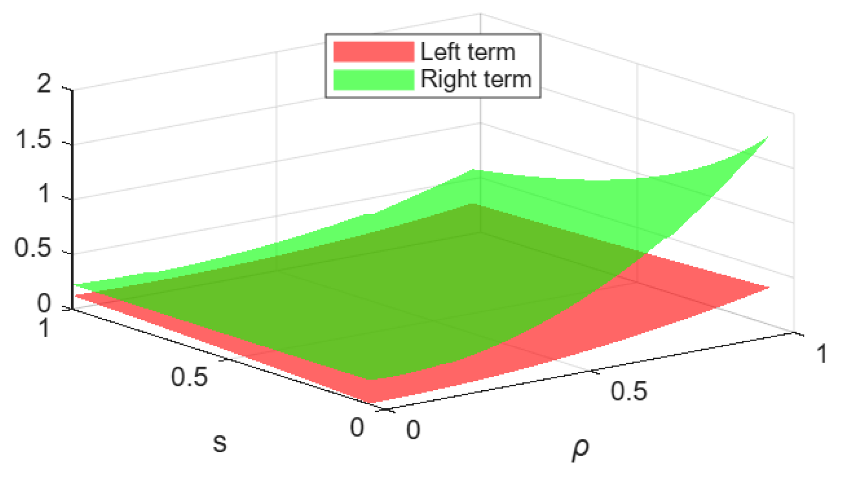
Figure 1 displays the left- and right-hand sides of inequality (18) over the domain $\varrho \in (0,1)$ and $s\in (0,1]$. As illustrated, the right-hand side consistently dominates the left-hand side, thereby supporting the correctness of the established inequality.

4.2. Applications

We further explore practical implications of our results, focusing on their potential use in error estimation for fractional quadrature formulas and in the analysis of numerical schemes involving proportional Caputo-hybrid operators. We begin by recalling the following special means of arbitrary real numbers ${\mathfrak{d}}_1$ and ${\mathfrak{d}}_2$:

$$\begin{array}{cc}\hfill \mathrm{Arithmetic}\mathrm{mean}:& \mathcal{A}({\mathfrak{d}}_1,{\mathfrak{d}}_2)={\displaystyle \frac{{\mathfrak{d}}_1+{\mathfrak{d}}_2}{2}},\hfill \\ \hfill \mathrm{Geometric}\mathrm{mean}:& \mathcal{G}({\mathfrak{d}}_1,{\mathfrak{d}}_2)=\sqrt{{\mathfrak{d}}_1{\mathfrak{d}}_2},\hfill \\ \hfill \mathrm{Harmonic}\mathrm{mean}:& \mathcal{H}({\mathfrak{d}}_1,{\mathfrak{d}}_2)={\displaystyle \frac{2{\mathfrak{d}}_1{\mathfrak{d}}_2}{{\mathfrak{d}}_1+{\mathfrak{d}}_2}},\hfill \\ \hfill \mathrm{Logarithmic}\mathrm{mean}:& \mathcal{L}({\mathfrak{d}}_1,{\mathfrak{d}}_2)={\displaystyle \frac{{\mathfrak{d}}_2-{\mathfrak{d}}_1}{\ln {\mathfrak{d}}_2-\ln {\mathfrak{d}}_1}},{\mathfrak{d}}_1,{\mathfrak{d}}_2>0\mathrm{with}{\mathfrak{d}}_1\ne {\mathfrak{d}}_2,\hfill \\ \hfill p\text{-}\mathrm{Logarithmic}\mathrm{mean}:& {\mathcal{L}}_p({\mathfrak{d}}_1,{\mathfrak{d}}_2)={\displaystyle \frac{{\mathfrak{d}}_2^{p+1}-{\mathfrak{d}}_1^{p+1}}{(p+1)({\mathfrak{d}}_2-{\mathfrak{d}}_1)}},{\mathfrak{d}}_1,{\mathfrak{d}}_2>0\mathrm{with}{\mathfrak{d}}_1\ne {\mathfrak{d}}_2\mathrm{and}p\in \mathbb{R}\setminus \{-1,0\}.\hfill \end{array}$$

Proposition 1.

Let ${\mathfrak{d}}_1,{\mathfrak{d}}_2\in \mathbb{R}$ with $0<{\mathfrak{d}}_1<{\mathfrak{d}}_2$, then we have

$$\left|{\displaystyle \frac{4}{3}}\mathcal{A}\left({\displaystyle \frac{1}{{\mathfrak{d}}_1}},{\displaystyle \frac{1}{{\mathfrak{d}}_2}}\right)-{\displaystyle \frac{1}{3{\mathcal{G}}^2\left({\mathfrak{d}}_1,{\mathfrak{d}}_2\right)}}\mathcal{H}\left({\mathfrak{d}}_1,{\mathfrak{d}}_2\right)-{\left({\mathfrak{d}}_2-{\mathfrak{d}}_1\right)}^2{\mathcal{L}}^{-1}\left({\mathfrak{d}}_1,{\mathfrak{d}}_2\right)\right|\le {\displaystyle \frac{{\mathfrak{d}}_2-{\mathfrak{d}}_1}{18}}\left(3+8{\left({\displaystyle \frac{1}{3}}\right)}^{\frac{1}{2}}\right){\mathcal{H}}^{-1}\left({\mathfrak{d}}_1^2,{\mathfrak{d}}_2^2\right).$$

Proof. 

Applying Corollary 4 to the function $\mathcal{F}\left(\varpi \right)=\ln \varpi$ yields

$$\left|{\displaystyle \frac{1}{3}}\left({\displaystyle \frac{2}{{\mathfrak{d}}_1}}-{\displaystyle \frac{2}{{\mathfrak{d}}_1+{\mathfrak{d}}_2}}+{\displaystyle \frac{2}{{\mathfrak{d}}_2}}\right)-{\displaystyle \frac{\ln {\mathfrak{d}}_2-\ln {\mathfrak{d}}_1}{{\mathfrak{d}}_2-{\mathfrak{d}}_1}}\right|\le {\displaystyle \frac{{\mathfrak{d}}_2-{\mathfrak{d}}_1}{108\sqrt{3}}}\left(9\sqrt{3}+24\right)\left({\displaystyle \frac{1}{{\mathfrak{d}}_1^2}}+{\displaystyle \frac{1}{{\mathfrak{d}}_2^2}}\right).$$

The assertion is obtained using the facts that

$${\displaystyle \frac{1}{2}}\left({\displaystyle \frac{1}{{\mathfrak{d}}_1}}+{\displaystyle \frac{1}{{\mathfrak{d}}_2}}\right)=\mathcal{A}\left({\displaystyle \frac{1}{{\mathfrak{d}}_1}},{\displaystyle \frac{1}{{\mathfrak{d}}_2}}\right),$$

$${\displaystyle \frac{2}{{\mathfrak{d}}_1+{\mathfrak{d}}_2}}={\displaystyle \frac{\mathcal{H}({\mathfrak{d}}_1,{\mathfrak{d}}_2)}{{\mathcal{G}}^2({\mathfrak{d}}_1,{\mathfrak{d}}_2)}},$$

$${\displaystyle \frac{\ln {\mathfrak{d}}_2-\ln {\mathfrak{d}}_1}{{\mathfrak{d}}_2-{\mathfrak{d}}_1}}={\mathcal{L}}^{-1}({\mathfrak{d}}_1,{\mathfrak{d}}_2),$$

and

$${\displaystyle \frac{1}{{\mathfrak{d}}_1^2}}+{\displaystyle \frac{1}{{\mathfrak{d}}_2^2}}=2{\mathcal{H}}^{-1}({\mathfrak{d}}_1,{\mathfrak{d}}_2).$$

□

Proposition 2.

Let ${\mathfrak{d}}_1,{\mathfrak{d}}_2\in \mathbb{R}$ with $0<{\mathfrak{d}}_1<{\mathfrak{d}}_2$ and $s\in (0,1]$, then we have

$$\left|4\mathcal{A}\left({\mathfrak{d}}_1^{s+1},{\mathfrak{d}}_2^{s+1}\right)-{\mathcal{A}}^{s+1}\left({\mathfrak{d}}_1,{\mathfrak{d}}_2\right)-3{\mathcal{L}}_{s+1}^{s+1}\left({\mathfrak{d}}_1,{\mathfrak{d}}_2\right)\right|\le {\displaystyle \frac{{\mathfrak{d}}_2-{\mathfrak{d}}_1}{s+2}}\left(2s+1+3{\left({\displaystyle \frac{1}{2}}\right)}^{s+1}\right)\left({\mathfrak{d}}_1^s+{\mathfrak{d}}_2^s\right).$$

Proof. 

Applying Corollary 2 to the function $\mathcal{F}\left(\varpi \right)={\varpi }^{s+1}$ yields

$$\left|{\displaystyle \frac{1}{3}}\left(2{\mathfrak{d}}_1^{s+1}-{\left({\displaystyle \frac{{\mathfrak{d}}_1+{\mathfrak{d}}_2}{2}}\right)}^{s+1}+2{\mathfrak{d}}_2^{s+1}\right)-{\displaystyle \frac{{\mathfrak{d}}_2^{s+2}-{\mathfrak{d}}_1^{s+2}}{(s+2)({\mathfrak{d}}_2-{\mathfrak{d}}_1)}}\right|\le {\displaystyle \frac{{\mathfrak{d}}_2-{\mathfrak{d}}_1}{s+2}}\left({\displaystyle \frac{2s+1}{3}}+2^{-(s+1)}\right)\left({\mathfrak{d}}_1^s+{\mathfrak{d}}_2^s\right).$$

The assertion is obtained by multiplying both sides of the above inequality by 3, and using the following equalities:

$${\displaystyle \frac{{\mathfrak{d}}_1^{s+1}+{\mathfrak{d}}_2^{s+1}}{2}}=\mathcal{A}\left({\mathfrak{d}}_1^{s+1},{\mathfrak{d}}_2^{s+1}\right),$$

$${\left({\displaystyle \frac{{\mathfrak{d}}_1+{\mathfrak{d}}_2}{2}}\right)}^{s+1}={\mathcal{A}}^{s+1}({\mathfrak{d}}_1,{\mathfrak{d}}_2),$$

and

$${\displaystyle \frac{{\mathfrak{d}}_2^{s+2}-{\mathfrak{d}}_1^{s+2}}{(s+2)({\mathfrak{d}}_2-{\mathfrak{d}}_1)}}={\mathcal{L}}_{s+1}^{s+1}({\mathfrak{d}}_1,{\mathfrak{d}}_2).$$

□

5. Conclusions

In this study, we have established Milne-type inequalities from the perspective of proportional Caputo-hybrid fractional operators. We treat the first- and second-order derivatives of the function as either convex or Lipschitz continuous. The inequalities derived from the regularity, be it geometric (convexity) or metric (Lipschitz), explain the error structure in fractional quadrature rules and also generalize classical results. The accompanying numerical experiment validates the sharpness of the theoretical bounds, and the suggested applications provide promising pathways in adaptive numerical integration and uncertainty quantification. This work contributes both methodologically and conceptually to the evolving interface between fractional calculus, functional inequalities, and computational mathematics.

References

1. Nápoles Valdés, J.E.; Rabossi, F.; Samaniego, A.D. Convex functions: Ariadne’s thread or Charlotte’s Spiderweb? Adv. Math. Model. Appl. 2020, 5, 176–191. [Google Scholar]
2. Niculescu, C.P. Convexity according to the geometric mean. Math. Inequal. Appl. 2020, 3, 155–167. [Google Scholar] [CrossRef]
3. Breckner, W.W. Stetigkeitsaussagen für eine Klasse verallgemeinerter konvexer Funktionen in topologischen linearen Räumen. Publ. Inst. Math. 1978, 23, 13–20. (In German) [Google Scholar]
4. Al-Sa’di, S.U.; Bibi, M.; Seol, Y.; Muddassar, M. Milne-type fractal integral inequalities for generalized m-convex mapping. Fractals 2023, 31, 2350081. [Google Scholar] [CrossRef]
5. Alomari, M. New error estimations for the Milne’s quadrature formula in terms of at most first derivatives. Konuralp J. Math. 2023, 1, 17–23. [Google Scholar]
6. Bosch, P.; Rodríguez, J.M.; Sigarreta, J.M. On new Milne-type inequalities and applications. J. Inequal. Appl. 2023, 2023, 3. [Google Scholar] [CrossRef]
7. Djenaoui, M.; Meftah, B. Milne type inequalities for differentiable s-convex functions. Honam Math. J. 2022, 44, 325–338. [Google Scholar]
8. Singh, P.; Mishra, S.K.; Kumar, P.; Hamdi, A. On some new Milne-type inequalities for strongly convex functions. Contemp. Math. 2025, 6, 3253–3268. [Google Scholar] [CrossRef]
9. Budak, H.; Kösem, P.; Kara, H. On new Milne-type inequalities for fractional integrals. J. Inequal. Appl. 2023, 2023, 10. [Google Scholar] [CrossRef]
10. Budak, H.; Hyder, A.A. Enhanced bounds for Riemann–Liouville fractional integrals: Novel variations of Milne inequalities. AIMS Math. 2023, 8, 30760–30776. [Google Scholar] [CrossRef]
11. Budak, H.; Karagözoğlu, P. Fractional Milne type inequalities. Acta Math. Univ. Comen. 2024, 93, 1–15. [Google Scholar]
12. Meftah, B.; Lakhdari, A.; Saleh, W. Milne-type inequalities for differentiable s-preinvex functions via Riemann–Liouville fractional integrals. Filomat 2024, 38, 9727–9742. [Google Scholar] [CrossRef]
13. Lakhdari, A.; Budak, H.; Awan, M.U.; Meftah, B. Extension of Milne-type inequalities to Katugampola fractional integrals. Bound. Value Probl. 2024, 2024, 100. [Google Scholar] [CrossRef]
14. Saleh, W.; Lakhdari, A.; Meftah, B. Some new Milne-type inequalities via Katugampola fractional integrals. Filomat 2025, 39, 8945–8959. [Google Scholar] [CrossRef]
15. Çelik, B.; Budak, H.; Set, E. On generalized Milne type inequalities for new conformable fractional integrals. Filomat 2024, 38, 1807–1823. [Google Scholar] [CrossRef]
16. Üneş, E.; Demir, İ. Error estimates for perturbed Milne-type inequalities by twice-differentiable functions using conformable fractional integrals. Bound. Value Probl. 2025, 2025, 73. [Google Scholar] [CrossRef]
17. Lakhdari, A.; Budak, H.; Mlaiki, N.; Meftah, B.; Abdeljawad, T. New insights on fractal–fractional integral inequalities: Hermite–Hadamard and Milne estimates. Chaos Solitons Fractals 2025, 193, 116087. [Google Scholar] [CrossRef]
18. Lakhdari, A.; Bin-Mohsin, B.; Achachera, K.; Xu, H.; Budak, H. On Milne-type inequalities via Katugampola fractional multiplicative integrals. Fractals 2026, 34, 2550116. [Google Scholar] [CrossRef]
19. Munir, A.; Qayyum, A.; Rathour, L.; Atta, G.; Supadi, S.S.; Ali, U. A study on Milne-type inequalities for a specific fractional integral operator with applications. Korean J. Math. 2024, 32, 297–314. [Google Scholar]
20. Baleanu, D.; Fernandez, A.; Akgul, A. On a fractional operator combining proportional and classical differintegrals. Mathematics 2020, 8, 360. [Google Scholar] [CrossRef]
21. Sarikaya, M.Z. On Hermite-Hadamard type inequalities for proportional Caputo-hybrid operator. Konuralp J. Math. 2023, 11, 31–39. [Google Scholar]
22. Sarikaya, M.Z. On Simpson type inequalities for proportional Caputo-hybrid operator. Int. J. Appl. Comput. Math. 2025, 11, 146. [Google Scholar] [CrossRef]
23. Demir, İ.; Tunç, T. Fractional Newton-type inequalities for twice differentiable functions via proportional Caputo-hybrid operator. Filomat 2025, 39, 7915–7938. [Google Scholar] [CrossRef]
24. Mehtab, M.; Butt, S.I.; Alammar, M.; Seol, Y. Caputo-hybrid fractional approach to estimates of corrected Euler–Maclaurin-type with computational analysis and applications. J. Inequal. Appl. 2026, 2026, 23. [Google Scholar] [CrossRef]
25. Demir, İ. A new approach of Milne-type inequalities based on proportional Caputo-Hybrid operator. J. Adv. App. Comput. 2023, 10, 102–119. [Google Scholar] [CrossRef]
26. Demir, İ. Milne-type inequalities for different classes of mapping based on proportional Caputo-hybrid operator. Turkish J. Ineq. 2023, 7, 47–61. [Google Scholar]
Figure 1. Visual illustration of Theorem 2.
Axioms 15 00280 g001
Disclaimer/Publisher’s Note: The statements, opinions and data contained in all publications are solely those of the individual author(s) and contributor(s) and not of MDPI and/or the editor(s). MDPI and/or the editor(s) disclaim responsibility for any injury to people or property resulting from any ideas, methods, instructions or products referred to in the content.