The Distribution and Quantiles of Sample Autocovariances and Autocorrelations of Sample Moments from a Stationary Process

Abstract

This paper gives expansions for the distribution, density and quantiles of any estimate that is a smooth function of the sample cross-moments of a stationary process. Three versions of these are given, depending on whether an exact, approximate, or asymptotic form is used for the variance or covariance of the estimate. Eight examples are provided, including sample autocovariances and autocorrelations. Their Central Limit Theorems extend those in the literature, such as Bartlett’s formula, by allowing for the effect of the mean and higher order cross-cumulants. Their distribution and quantiles are given to magnitude $n^{-r/2}$ up to r = 3, where n is the sample size.

1. Introduction and Summary

Traditionally, time series use models such as moving average and autoregressive models. The danger of such parametric models is that if the wrong model is chosen, the results will be wrong as well. It is of crucial importance for the asymptotic variance to be correct. Otherwise, the model will not even give asymptotic accuracy. Here, I take a nonparametric approach. The degree of accuracy available is limited to the cases where the results of [1] can be applied, that is, when the total order of the cross-cumulants is less than nine. For example, this allows the computation of the asymptotic variance and the Central Limit Theorem (CLT) for the sample autocovariance as well as its distribution and quantiles to magnitude $n^{-1}$, written as $O\left(n^{-1}\right)$, where n is the sample size. This is also the first time a nonparametric CLT has been given for the sample autocorrelation. For higher-order accuracy, or when the number of terms is large, software may be needed to apply or extend [1], as spelt out in Appendix B.

CLTs for the sample mean from a stationary series, $\left\{X_t\right\}$, were given in Chapter 4 of [2], Chapter 18 of [3], and some of my own papers.

Let $\left\{X_t\right\}$ be a stationary series.

$$\mathrm{Set} \mu =E{X}_0 \mathrm{and} {\gamma }_t=covar(X_0,X_t)=E(X_0-\mu )(X_t-\mu ),$$

the autocovariance. Let $\overline{X}$ be the mean of $X_1, \dots , X_n$. Then, under regularity conditions,

$${\kappa }_2=nvar\left(\overline{X}\right)=\sum _{\left|T\right|<n}(1-|T|/n){\gamma }_T=a_{21}+n^{-1}{a}_{22}, \mathrm{say},$$

(1)

$$\to {\overline{\kappa }}_2=\sum _{\left|T\right|<\infty }{\gamma }_T, \mathrm{and} n^{1/2}(\overline{X}-\mu )\stackrel{\mathcal{L}}{\to }\mathcal{N}(0,{\overline{\kappa }}_2) \mathrm{as} n\to \infty ,$$

(2)

the normal distribution. We call $a_{21}={\sum }_{\left|T\right|<n}{\gamma }_T$ and ${\overline{\kappa }}_2$ of (2) the approximate variance and the asymptotic variance of $n^{1/2}(\overline{X}-\mu )$. It was not until [4] that this result for $\overline{X}$ was extended to Edgeworth–Cornish–Fisher (ECF) expansions, that is, the expansions in powers of $n^{-1/2}$ for its distribution, density and quantiles. Ref. [5] did give these for smooth functions of the sample cross-moments of a linear process, and ref. [4] extended these results to a general stationary process. For any $I \ge 2,$ I give the Ith-order ECF expansions for $\overline{X}$, that is, these expansions to $O\left(n^{-I/2}\right)$, in terms of the cross-cumulants of $\left\{X_t\right\}$ up to order $I + 1$.

For any smooth function of sample cross-moments, this paper gives three types of ECF expansions: (1) the mean-type expansions, i.e., those about the normal using the exact variance, when this is available (${\kappa }_2$ of (1) in the case of the sample mean); (2) the standard-type expansions, i.e., those about the normal using the approximate variance ($a_{21}$ of (1) in the case of $\overline{X}$); and (3) the asymptotic-type expansions, i.e., those about the normal using the asymptotic variance (${\overline{\kappa }}_2$ of (1) in the case of $\overline{X}$). For $\overline{X}$, these were given only recently, in [4]: for $I \ge 3$, they use ${\kappa }_r = n^{r-1}{\kappa }_r\left(\overline{X}\right)$ for $r \le I + 1$.

Now suppose that $\widehat{\theta }$ is a standard estimator based on a sample of size n of an unknown parameter $\theta \in R^q$ in a statistical model. That is, $E\widehat{\theta }\to \theta$ as $n\to \infty ,$ and for $r \ge 1$, its rth-order cross-cumulants are $O\left(n^{1-r}\right)$ and can be expanded in powers of $n^{-1}$, with explicit forms for the coefficients needed in these expansions. (The classic example is when $\widehat{\theta }$ is a smooth function of a sample mean.) Then ECF expansions are available for its distribution that improve upon the first-order expansions, that is, the CLT. In order to be self-contained, Section 2 summarises these ECF expansions to $O\left(n^{-2}\right)$.

Per [6], smooth functions of a standard estimator, such as the sample cross-cumulants and functions of them, are also standard estimators. Thus, these also have the ECF expansions described in Section 2.

Section 3 gives the cumulant coefficients for a function of an unbiased standard estimator that are needed for the third-order ECF expansions.

In Section 4, I show that the sample non-central cross-moments of a stationary process are unbiased standard estimators. (In fact, their cumulant expansions have exactly two terms.)

The most important functions of cross-cumulants, are the sample autocovariance, ${\widehat{\gamma }}_a$, and the sample autocorrelation, ${\widehat{\rho }}_a={\widehat{\gamma }}_a/{\widehat{\gamma }}_0$. These have been useful tools in time series since [7]: see [8].

Corollary 1 gives three choices for the cumulant coefficients needed for these expansions: their mean-type values, their approximate values and their asymptotic values. These are given in terms of cross-cumulants that I call the K functions.

Applications of stationary time series fall into two classes. The first class, dealt with in Section 5, is when the mean, $\mu$, is zero. This includes many branches of radio, radar, sonar, speech, image analysis, communications, control and seismology. This class is dealt with much more easily than the second class, stationary series with an unknown mean. For example, the autocovariance is a cross-cumulant if the mean is zero, but otherwise it is a function of two cross-cumulants.

Section 6, Section 7, Section 8, Section 9 and Section 10 deal with the second class, that is, when $\mu$ is unknown. Section 6 gives the ECF expansions for the distribution to any order I of $\overline{X}$. Section 7 gives the ECF expansions for the distribution to order two of the sample autocovariance (${\widehat{\gamma }}_a$). Section 8 gives the ECF expansions to order one (the CLT) for the sample autocorrelation (${\widehat{\rho }}_a$). An exact form is given for $nvar({\widehat{\gamma }}_a$) but is not available for $nvar\left({\widehat{\rho }}_a\right)$. Corollaries 3 and 4 spell out for the first time how the asymptotic variances of the sample autocovariance and the sample autocorrelation depend on the mean and cross-cumulants up to order four. Section 9 gives multivariate CLTs for $({\widehat{\gamma }}_0, \dots , {\widehat{\gamma }}_a)$ and $({\widehat{\rho }}_1, \dots , {\widehat{\rho }}_a)$. These extensions of (1) and (2) are all new. However, the examples go beyond CLTs: they provide the distribution, density and quantiles of the estimates up to order I, $O\left(n^{-I/2}\right)$, for various I.

Other important examples are the sample versions of the autocovariances of degree $r \ge 2$,

$${\gamma }_{t_2,\dots ,t_r}=cov(X_0,X_{t_2},\dots ,X_{t_r})=E(X_0-\mu )(X_{t_2}-\mu )\dots ,(X_{t_r}-\mu ),$$

(3)

and their autocorrelations. These have not been studied for $r > 2$, perhaps because for odd values of r they are zero for a Gaussian process. CLTs for ${\widehat{\gamma }}_{t,s}$ are given in Example 4 for $\mu = 0$ and in Section 10 for $\mu \ne 0$.

Section 11 shows how to extend the results of Section 4 to a multivariate stationary process. Section 12 discusses our results and identifies some future directions worth pursuing.

Appendix A applies Appendix B to give the cross-cumulant functions, the K functions, needed for the examples in Section 5, Section 6, Section 7, Section 8, Section 9 and Section 10. Appendix B explicitly states the leading cross-cumulants implicit in [1].

As noted, our nonparametric approach gives an alternative to traditional parametric time series models, such as a moving average (MA), autoregressive (AR), or ARMA process. Another difficulty with such parametric models is estimating their parameters. A vast collection of software has been developed for economists and others to use for this purpose. Potentially, these parametric time series models and the software for them could be replaced by the nonparametric method given here, where the results of [1] can be applied or extended to the desired degree of accuracy.

This paper does not deal with observations that have a signal beyond the mean (for example, $E{X}_t = a + bt$ or a sinusoidal signal.) Furthermore, I do not provide software to help with the large number of terms sometimes needed.

Turning to the literature on ECF expansions, refs. [9,10,11] showed that Cornish–Fisher expansions gave substantial improvements to the CLT, even for lattice estimators such as the binomial and Poisson estimators. Ref. [12] presented an extension to nonstationary processes. Ref. [13] obtained an Edgeworth correction by bootstrapping in autoregressions. Ref. [14] gave an Edgeworth expansion for U-statistics with dependent observations. Ref. [15] used an Edgeworth expansion to study empirical likelihood methods for dependent processes. For a review of a paper by Taniguchi and Kakizawa on Edgeworth and saddlepoint expansions for time series, see [16]. Ref. [17] gave expansions for a maximum likelihood estimator for a stationary Gaussian process.

See [7,18,19,20,21,22,23,24] for consistency and some theory and applications. The variance formula of [7] can produce invalid confidence intervals: see [25,26,27]. This is not surprising because it neglects the mean and higher-order cumulants.

Ref. [28] gave an Edgeworth expansion for ${\widehat{\rho }}_a$ under long-range dependence. Ref. [29] gave an Edgeworth expansion for the maximum likelihood estimator of a stationary long-memory Gaussian time series.

Note 1.

Refs. [5,30] considered the general stationary linear process

$$X_t=\sum _{j=0}^{\infty }{\rho }_j{e}_{t-j}$$

(4)

where $\left\{{\rho }_j\right\}$ are constants, while $e_0,e_1,\dots ,$ are independent and identically distributed (i.i.d.) random variables from a distribution on R with finite cumulants $\left\{{\tau }_j\right\}$. Its cross-cumulants were shown to be

$$\mu =E{X}_0={\tau }_1\sum _{j=0}^{\infty }{\rho }_j,\kappa (X_{t_1},\dots ,X_{t_r})=\alpha (t_1,\cdots t_r){\tau }_r, for r\ge 2$$

(5)

$$where \alpha (t_1,\cdots ,t_r)=\sum _{j=0}^{\infty }{\rho }_{j+t_1}\cdots {\rho }_{j+t_r},$$

and that $\alpha (t_1,\cdots ,t_r)$ is finite for processes such as ARMA where ${\rho }_j\to 0$ exponentially as $n\to \infty .$

See [5] for a simulation study. For an autoregressive process $\left\{X_j\right\}$, see p. 158 of [5].

Ref. [31] considered the model

$$X_t=\mu +\sum _{j=-\infty }^{\infty }{\rho }_j{e}_{t-j},$$

where $\left\{{\rho }_j\right\}$ are constants, while $\left\{e_t\right\}$ are i.i.d. with finite cumulants $\left\{{\tau }_j\right\}$ where ${\tau }_1 = 0$. In this case, (5) holds with

$$\alpha (t_1,\cdots ,t_r)=\sum _{j=-\infty }^{\infty }{\rho }_{j+t_1}\cdots {\rho }_{j+t_r}.$$

2. ECF Expansions for Standard Estimators

This section summarises the Edgeworth–Cornish–Fisher expansions that can be found in [32,33].

Univariate estimators. Suppose that $\widehat{\theta }$ is a standard estimator of an unknown $\theta \in R$ with respect to n, typically the sample size. That is, $E\widehat{\theta }\to \theta$ as $n\to \infty$, and its cumulants can be expanded as

$$\begin{array}{c}{\kappa }_r(\widehat{\theta })={\displaystyle \sum _{j=r-1}^{I-1}}{n}^{-j}{a}_{rj}+O\left(n^{-I}\right) \mathrm{for} I\ge r\ge 1,\hfill \\ \approx {\displaystyle \sum _{j=r-1}^{\infty }}{n}^{-j}{a}_{rj} \mathrm{for} r\ge 1,\hfill \end{array}$$

(6)

where the cumulant coefficients $a_{rj}$ may depend on n but are bounded as $n\to \infty$, $a_{21}$ is bounded away from 0, and $y_n = O\left(x_n\right)$ means that $y_n/x_n$ is bounded in n. Here and below, ≈ indicates an asymptotic expansion that need not converge. For non-lattice $\widehat{\theta }$, the distribution and quantiles of

$$Y_n={(n/a_{21})}^{1/2}(\widehat{\theta }-\theta )$$

(7)

have expansions in powers of $n^{-1/2}$ of the form

$$\begin{array}{c}{P}_n\left(x\right)=Prob(Y_n\le x)=\Phi \left(x\right)-\varphi \left(x\right){\displaystyle \sum _{r=1}^{I-1}}{n}^{-r/2}{h}_r\left(x\right)+O\left(n^{-I/2}\right)\hfill \\ \approx \Phi \left(x\right)-\varphi \left(x\right){\displaystyle \sum _{r=1}^{\infty }}{n}^{-r/2}{h}_r\left(x\right),\hfill \end{array}$$

(8)

$$\begin{array}{c}{p}_n\left(x\right)=d{P}_n\left(x\right)/dx=\varphi \left(x\right)[1+{\displaystyle \sum _{r=1}^{I-1}}{n}^{-r/2}{\overline{h}}_r\left(x\right)]+O\left(n^{-I/2}\right)\hfill \\ \approx \varphi \left(x\right)[1+{\displaystyle \sum _{r=1}^{\infty }}{n}^{-r/2}{\overline{h}}_r\left(x\right)],\hfill \end{array}$$

(9)

$$\begin{array}{c}{\Phi }^{-1}\left(P_n\left(x\right)\right)=x-{\displaystyle \sum _{r=1}^{I-1}}{n}^{-r/2}{f}_r\left(x\right)+O\left(n^{-I/2}\right)\hfill \\ \approx x-{\displaystyle \sum _{r=1}^{\infty }}{n}^{-r/2}{f}_r\left(x\right),\hfill \end{array}$$

(10)

$$\begin{array}{c}{P}_n^{-1}(\Phi \left(x\right))=x+{\displaystyle \sum _{r=1}^{I-1}}{n}^{-r/2}{g}_r\left(x\right)+O\left(n^{-I/2}\right)\hfill \\ \approx x+{\displaystyle \sum _{r=1}^{\infty }}{n}^{-r/2}{g}_r\left(x\right),\hfill \end{array}$$

(11)

where $\Phi \left(x\right) = Prob(N \le x),N\sim \mathcal{N}(0, 1)$ is a unit normal random variable with density $\varphi \left(x\right) = {\left(2\pi \right)}^{-1/2}{e}^{-x^2/2}$; $h_r\left(x\right), {\overline{h}}_r\left(x\right), f_r\left(x\right), g_r\left(x\right)$ are polynomials in x and $\left\{A_{ri}\right\}$; and

$$A_{ri}=a_{ri}/a_{21}^{r/2}.$$

(12)

I call these the Ith-order ECF expansions. They are given in [32] to order five, that is, to $O\left(n^{-5/2}\right)$, starting as follows:

$$h_1\left(x\right)=f_1\left(x\right)=g_1\left(x\right)=A_{11}+A_{32}{H}_2/6,{\overline{h}}_1\left(x\right)=A_{11}{H}_1+A_{32}{H}_3/6,$$

(13)

$$h_2\left(x\right)=(A_{11}^2+A_{22})H_1/2+(A_{11}{A}_{32}+A_{43}/4)H_3/6+A_{32}^2{H}_5/72,$$

(14)

$$f_2\left(x\right)=(A_{22}/2-A_{11}{A}_{32}/3)H_1+A_{43}{H}_3/24-A_{32}^2(4x^3-7x)/36,$$

$$g_2\left(x\right)=A_{22}{H}_1/2+A_{43}{H}_3/24-A_{32}^2(2x^3-5x)/36,$$

$${\overline{h}}_2\left(x\right)=(A_{11}^2+A_{22})H_2/2+(A_{11}{A}_{32}+A_{43}/4)H_4/6+A_{32}^2{H}_6/72,$$

(15)

where, for $k\ge 0,H_k$ is the kth Hermite polynomial,

$$\begin{array}{c}{H}_k=H_k\left(x\right)=\varphi {\left(x\right)}^{-1}{(-d/dx)}^k\varphi \left(x\right):\hfill \\ H_0=1,H_1=x,H_2=x^2-1,H_3=x^3-3x,H_4=x^4-6x^2+3,\dots \hfill \end{array}$$

Thus, (8)–(15) give the Ith-order ECF expansions for the distribution, density and quantiles of $Y_n$ of (7), in terms of $a_{21}$ for $I = 1$; in terms of $a_{21}, a_{11}, a_{32}$ for $I = 2$; and in terms of $a_{21}, a_{11}, a_{32}, a_{22}, a_{43}$ for $I = 3.$

Note 2.

Refs. [34,35] gave (11) for $I \le 6$ for a special case. Their results were extended to standard estimators in [32]. In their examples, (11) gave quantiles to a large number of decimal places. However, for small enough n, divergence can start after the first or second term. In practice, one terminates (8)–(11) if they start to diverge.

Mean-type univariate estimators. We say that $\widehat{w}$ is a mean-type estimator if $E\widehat{w} = w$ and, for $r \ge 1,$ its rth cumulant has magnitude $n^{1-r}$, say,

$${\kappa }_r\left(\widehat{w}\right)=n^{1-r}{\kappa }_r,$$

where ${\kappa }_r$ is bounded as $n\to \infty$. (The classic example is when $\widehat{w}$ is the mean of a random sample from a distribution on R with mean w and rth cumulant ${\kappa }_r,r \ge 1$.) For this special type of standard estimator, the above results simplify. If $a_{r,r-1}$ is replaced with ${\kappa }_r$ and other $a_{ri}$ are replaced with zero, then $A_{r,r-1} = {\kappa }_r/{\kappa }_2^{r/2},$ and $A_{11} = A_{22} = 0$ in (13)–(15).

Multivariate estimators. Set

$${\varphi }_V\left(x\right)={\left(2\pi \right)}^{-q/2}{\left(det\left(V\right)\right)}^{-1/2}exp(-x^{\prime }{V}^{-1}x/2),{\Phi }_V\left(x\right)={\int }_{-\infty }^x{\varphi }_V\left(x\right)dx,$$

the density and distribution of the multivariate normal $X\sim {\mathcal{N}}_p(0,V)$.

I now reserve $i_1,i_2,\dots$ for any sequence from $1,2,\dots ,p$. To avoid double subscripts, I introduce the bar notation.

The multivariate Hermite polynomial, ${\overline{H}}^{1-k} = {\overline{H}}^{1-k}(x,V)$$= H^{i_1\dots i_k}$, is

$$\begin{array}{c}{\overline{H}}^{1-k}={\varphi }_V{\left(x\right)}^{-1}(-{\overline{\partial }}_1)\dots (-{\overline{\partial }}_k){\varphi }_V\left(x\right),\mathrm{where} {\partial }_i=\partial /\partial x_i \mathrm{and} {\overline{\partial }}_k={\partial }_{i_k}:\hfill \\ H^1=y_1,{\overline{H}}^1={\overline{y}}_1,H^{12}=y_1{y}_2-V^{12},{\overline{H}}^{12}={\overline{y}}_1{\overline{y}}_2-{\overline{V}}^{12},\hfill \\ H^{1-3}=y_1{y}_2{y}_3-{\displaystyle \sum ^3}{V}^{12}{y}_3, \mathrm{where} {\displaystyle \sum ^3}{V}^{12}{y}_3=V^{12}{y}_3+V^{13}{y}_2+V^{23}{y}_1,\hfill \end{array}$$

while ${\overline{V}}^{12} = V^{i_1{i}_2}$ is the $(i_1,i_2)$ element of $V^{-1}.$ Their integrated form is

$${\overline{H}}_{\ast }^{1-k}=H_{\ast }^{i_1\dots i_k}=(-{\overline{\partial }}_1)\dots (-{\overline{\partial }}_k){\Phi }_V\left(x\right)={\int }_{-\infty }^x{\overline{H}}^{1-k}{\varphi }_V\left(x\right)dx.$$

Now suppose that $\widehat{w}$ is a standard estimator of $w\in R^p$ with respect to n. That is, $E\widehat{w}\to w$ as $n\to \infty$, and for $r \ge 1$, $1 \le i_1,\dots ,i_r \le p,$ the rth order cumulants of $\widehat{w}$ can be expanded as

$$\kappa ({\widehat{w}}_{i_1},\dots ,{\widehat{w}}_{i_r})\approx \sum _{j=r-1}^{\infty }{n}^{-j}{\overline{k}}_j^{1-r} \mathrm{where} {\overline{k}}_j^{1-r}=k_j^{i_1\dots i_r},$$

(16)

and the cumulant coefficients ${\overline{k}}_j^{1-r}$ may depend on n but are bounded as $n\to \infty$. Therefore, ${\overline{k}}_0^1 = {\overline{w}}_1 = w_{i_1}.$ Then,

$$X_n=n^{1/2}(\widehat{w}-w)\stackrel{\mathcal{L}}{\to }X\sim {\mathcal{N}}_p(0,V) \mathrm{where} V=\left(k_1^{i_1{i}_2}\right),p\times p.$$

(17)

V may depend on n, but I assume that $det\left(V\right)$ is bounded away from zero. By [6], the distribution and density of $X_n = n^{1/2}(\widehat{w} - w)$ can be expanded as

$$Prob.(X_n\le x)=\sum _{r=0}^{I-1}{n}^{-r/2}{P}_r\left(x\right)+O\left(n^{-I/2}\right)\approx \sum _{r=0}^{\infty }{n}^{-r/2}{P}_r\left(x\right),$$

(18)

$$p_{X_n}\left(x\right)=\sum _{r=0}^{I-1}{n}^{-r/2}{p}_r\left(x\right)+O\left(n^{-I/2}\right)\approx \sum _{r=0}^{\infty }{n}^{-r/2}{p}_r\left(x\right),x\in R^p,$$

(19)

where $P_0\left(x\right) = {\Phi }_V\left(x\right),p_0\left(x\right) = {\varphi }_V\left(x\right),$ and for $r \ge 1,$

$$P_r\left(x\right)=\sum _{k=1}^{3r}[{\overline{P}}_r^{1-k}{\overline{H}}_{\ast }^{1-k}(x,V):k-r \mathrm{even}],$$

(20)

$$p_r\left(x\right)/{\varphi }_V\left(x\right)=\sum _{k=1}^{3r}[{\overline{P}}_r^{1-k}{\overline{H}}^{1-k}(x,V):k-r-\mathrm{even}]={\tilde{p}}_r\left(x\right), \mathrm{say}.$$

(21)

Statements (20) and (21) use the tensor summation convention of implicitly summing $i_1,\dots ,i_k$ over their range $1,\dots ,p$. The coefficients ${\overline{P}}_r^{1-k}$ are called the Edgeworth coefficients. These are polynomials in the cumulant coefficients ${\overline{k}}_j^{1-r}$ of (16). See [33] for their definition. There, I show that the Edgeworth coefficients needed for Edgeworth expansions to order three, that is, to $O\left(n^{-3/2}\right)$, are

$$\begin{array}{c}{\overline{P}}_1^1={\overline{k}}_1^1,{\overline{P}}_1^{1-3}={\overline{k}}_2^{1-3}/6,{\overline{P}}_2^{12}={\overline{k}}_1^1{\overline{k}}_1^2+{\overline{k}}_2^{12}/2,\hfill \\ {\overline{P}}_2^{1-4}={\overline{k}}_3^{1-4}/24+\mathcal{S}{\overline{k}}_1^1{\overline{k}}_2^{2-4}/6+\mathcal{S}{\overline{k}}_1^4{\overline{k}}_2^{1-3}/6,{\overline{P}}_2^{1-6}=\mathcal{S}{\overline{k}}_2^{1-3}{\overline{k}}_2^{4-6}/36,\hfill \end{array}$$

where $\mathcal{S}$ is the operator that symmetrizes ${\overline{f}}^{1-k} = f^{i_1\dots ,i_k}$. Thus,

$$\begin{array}{c}{P}_1\left(x\right)={\overline{k}}_1^1{\overline{H}}_{\ast }^1(x,V)+{\overline{k}}_2^{1-3}{\overline{H}}_{\ast }^{1-3}(x,V)/6,\hfill \\ {\tilde{p}}_1\left(x\right)={\overline{k}}_1^1{\overline{H}}^1(x,V)+{\overline{k}}_2^{1-3}{\overline{H}}^{1-3}(x,V)/6,\hfill \\ P_2\left(x\right)={\displaystyle \sum _{k=2,4,6}}{\overline{P}}_2^{1-k}{\overline{H}}_{\ast }^{1-k}(x,V),{\tilde{p}}_2\left(x\right)={\displaystyle \sum _{k=2,4,6}}{\overline{P}}_2^{1-k}{\overline{H}}^{1-k}(x,V).\hfill \end{array}$$

For ${\overline{P}}_3^{1-k}$ and more details, see [33]. These give the Edgeworth expansions for the distribution of $X_n = n^{1/2}(\widehat{w} - w)$ to order four, that is, to $O\left(n^{-2}\right)$, for non-lattice $\widehat{w}$.

ECF expansions for parametric and nonparametric standard estimators were first given in [32].

In Section 4, I show that for the sample cross-moments of a stationary time series, only the first two terms in (6) and (16) are non-zero for $r \ge 2.$

Mean-type multivariate estimators. We say that $\widehat{w}$ is a mean-type estimator if $E\widehat{w} = w$ and, for $r \ge 1,$ its rth-order cumulants have magnitude $n^{1-r}$, say,

$$\kappa ({\widehat{w}}_1,\dots ,{\widehat{w}}_r)=n^{1-r}{\kappa }^{1\dots r},$$

where ${\kappa }^{1\dots r}$ is bounded as $n\to \infty$. (The classic example is when $\widehat{w}$ is the mean of a random sample from a distribution on $R^p$ with mean w and rth-order cumulants ${\kappa }^{1\dots r}$.) For this special type of standard estimator, the above results simplify. If ${\overline{k}}_{r-1}^{1-r}$ is replaced ${\overline{\kappa }}^{1-r}={\kappa }^{i_1\dots i_r}$ and other ${\overline{k}}_j^{1-r}$ are replaced with zero, then (18)–(21) hold with

$$\begin{array}{c}{\overline{P}}_1^1=0,{\overline{P}}_1^{1-3}={\overline{\kappa }}^{1-3}/6,\hfill \\ {\overline{P}}_2^{12}=0,{\overline{P}}_2^{1-4}={\overline{\kappa }}^{1-4}/24,{\overline{P}}_2^{1-6}=\mathcal{S}{\overline{\kappa }}^{1-3}{\overline{\kappa }}^{4-6}/36.\hfill \end{array}$$

That is, the classic Edgeworth expansions for a sample mean can be applied with this re-interpretation of ${\overline{\kappa }}^{1-r}$.

3. Cumulant Coefficients for Functions of Unbiased Standard Estimators

This section summarises the results from [6] needed in Section 5.

Suppose that $\widehat{w}\in R^p$ is a standard estimator satisfying (16) and that

$$\begin{array}{c}\hfill \theta =t\left(w\right):R^p\to R^q\end{array}$$

(22)

is a smooth function with finite derivatives

$$\begin{array}{c}\hfill t_{\blacksquare a_1{a}_2\dots }={\partial }_{a_1}{\partial }_{a_2}\cdots t\left(w\right) \mathrm{where} {\partial }_a=\partial /\partial w_a.\end{array}$$

(23)

For $b = 1, \cdots , q$, let ${\theta }^b = t^b\left(w\right)$ be the bth component of $\theta$. Then, by [6], $\widehat{\theta } = t\left(\widehat{w}\right)$ is a standard estimator of $\theta = t\left(w\right)$. Thus, its rth-order cross-cumulants are of magnitude $n^{1-r}$ with an expansion of the form

$$\kappa ({\widehat{\theta }}^{b_1},\cdots ,{\widehat{\theta }}^{b_r})\approx \sum _{j=r-1}^{\infty }{n}^{-j}{K}_{nj}^{b_1\cdots b_r}$$

(24)

where $b_1, \cdots b_r$ lie in $1, \cdots , q,K_{n0}^b = {\theta }^b,$ and the cumulant coefficients for $\widehat{\theta },K_{nj}^{b_1\cdots b_r}$, are given in terms of the cumulant coefficients for $\widehat{w},\{{\overline{k}}_j^{1-r}=k_j^{i_1\dots i_r}\}$ of (16) and the derivatives $t_{\blacksquare a_1{a}_2\dots }$, in Theorem 2 of [32], where I now assume that $E\widehat{w} = w$. Thus,

$$Z_n=n^{1/2}(\widehat{\theta }-\theta )\stackrel{\mathcal{L}}{\to }{\mathcal{N}}_q(0,\tilde{V})as n\to \infty \mathrm{where} \tilde{V}=(K_{n1}^{b_1{b}_2}),$$

(25)

$$\mathrm{and} K_{n1}^{b_1{b}_2}=t_{\blacksquare a_1}^{b_1}{k}_1^{a_1{a}_2}{t}_{\blacksquare a_2}^{b_2},$$

(26)

where, again, I use the tensor summation convention of implicit summation of the repeated pairs, in this case $a_1$ and $a_2$, over their range $1, \cdots , p$. That is,

$$K_{n1}^{b_1{b}_2}=\sum _{a_1,a_2=1}^p{t}_{\blacksquare a_1}^{b_1}{k}_1^{a_1{a}_2}{t}_{\blacksquare a_2}^{b_2}.$$

I call $\tilde{V} = \left(K_{n1}^{b_1{b}_2}\right)$ the approximate covariance or the asymptotic covariance, depending on whether an approximate or asymptotic value is used for $k_1^{a_1{a}_2}$. Similarly, $K_{n1}^{b_1} = t_{\blacksquare a_1{a}_2}^{b_1}{k}_1^{a_1{a}_2}/2$ is the tensor form for $K_{n1}^{b_1} = {\sum }_{a_1,a_2=1}^p{t}_{\blacksquare a_1{a}_2}^{b_1}{k}_1^{a_1{a}_2}/2.$ Furthermore,

$$K_{n2}^{b_1{b}_2{b}_3}=t_{\blacksquare a_1}^{b_1}{t}_{\blacksquare a_2}^{b_2}{t}_{\blacksquare a_3}^{b_3}{k}_2^{a_1{a}_2{a}_3}+\sum _{b_1{b}_2{b}_3}^3{s}_{a_1}^{b_1}{t}_{\blacksquare a_1{a}_3}^{b_2}{s}_{a_3}^{b_3} \mathrm{where} s_{a_1}^{b_1}=k_1^{a_1{a}_2}{t}_{\blacksquare a_2}^{b_1},$$

(27)

$$\begin{array}{c}{K}_{n2}^{b_1{b}_2}=t_{\blacksquare a_1}^{b_1}{t}_{\blacksquare a_2}^{b_2}{k}_2^{a_1{a}_2}+{\displaystyle \sum _{b_1{b}_2}^2}[t_{\blacksquare a_1{a}_2}^{b_1}{t}_{\blacksquare a_3}^{b_2}{k}_2^{a_1{a}_2{a}_3}+t_{\blacksquare a_1{a}_2{a}_3}^{b_1}{s}_{a_3}^{b_2}{k}_1^{a_1{a}_2}]/2\hfill \\ +v_{a_3}^{b_1{a}_2}{v}_{a_2}^{b_2{a}_3}/2 \mathrm{where} v_{a_3}^{b_1{a}_2}=t_{\blacksquare a_1{a}_3}^{b_1}{k}_1^{a_1{a}_2},\hfill \\ K_{n3}^{b_1\dots b_4}=t_{\blacksquare a_1}^{b_1}\dots t_{\blacksquare a_4}^{b_4}{k}_3^{a_1\dots a_4}+k_2^{a_1{a}_2{a}_3}{\displaystyle \sum ^{12}}{t}_{\blacksquare a_2}^{b_2}{t}_{\blacksquare a_3}^{b_3}{u}_{a_1}^{b_1{b}_4}+{\displaystyle \sum ^4}{t}_{\blacksquare a_1{a}_3{a}_5}^{b_1}{s}_{a_1}^{b_2}{s}_{a_3}^{b_3}{s}_{a_5}^{b_4}\hfill \\ +{\displaystyle \sum ^{12}}{u}_{a_1}^{b_1{b}_3}{k}_1^{a_1{a}_2}{u}_{a_2}^{b_2{b}_4} \mathrm{where} u_{a_1}^{b_1{b}_4}=t_{\blacksquare a_1{a}_4}^{b_1}{s}_{a_4}^{b_4}.\hfill \end{array}$$

These are the cumulant coefficients needed for $P_r\left(x\right),p_r\left(x\right)$ of (18) for $r=1,2$ when $X_n$ of (17) is replaced with $Z_n$ of (25). That is, these give the distribution and density of $Z_n=n^{1/2}(t\left(\widehat{w}\right)-t\left(w\right))$ to $O\left(n^{-3/2}\right)$ for non-lattice $\widehat{w}$.

The case q = 1. By (6), one can replace $K_{nj}^{b_1\dots b_r}$ with $a_{rj}$, where, by (24)–(27),

$$a_{10}=\theta ,a_{21}=t_{\blacksquare a_1}{k}_1^{a_1{a}_2}{t}_{\blacksquare a_2}=t_{\blacksquare a_1}{s}_{a_1} \mathrm{for} s_{a_1}=k_1^{a_1{a}_2}{t}_{\blacksquare a_2},$$

(28)

$$a_{11}=t_{\blacksquare a_1{a}_2}{k}_1^{a_1{a}_2}/2,a_{32}=t_{\blacksquare a_1}{t}_{\blacksquare a_2}{t}_{\blacksquare a_3}{k}_2^{a_1{a}_2{a}_3}+3s_{a_1}{t}_{\blacksquare a_1{a}_3}{s}_{a_3},$$

(29)

$$a_{22}=t_{\blacksquare a_1}{k}_2^{a_1{a}_2}{t}_{\blacksquare a_3}+t_{\blacksquare a_1{a}_2}{k}_2^{a_1{a}_2{a}_3}{t}_{\blacksquare a_3}+s_{a_3}{t}_{\blacksquare a_1{a}_2{a}_3}{k}_1^{a_1{a}_2}+v_{a_3}^{a_2}{v}_{a_2}^{a_3},$$

(30)

$$\begin{array}{c}{a}_{43}=t_{\blacksquare a_1}\dots t_{\blacksquare a_4}{k}_3^{a_1\dots a_4}+12u_{a_1}{k}_2^{a_1{a}_2{a}_3}{t}_{\blacksquare a_2}{t}_{\blacksquare a_3}+4t_{\blacksquare a_1{a}_3{a}_5}{s}_{a_1}{s}_{a_3}{s}_{a_5}\hfill \\ +12u_{a_1}{k}_1^{a_1{a}_2}{u}_{a_2} \mathrm{for} v_{a_3}^{a_2}=t_{\blacksquare a_1{a}_3}{k}_1^{a_1{a}_2},u_{a_1}=t_{\blacksquare a_1{a}_2}{s}_{a_2}.\hfill \end{array}$$

(31)

These are the $a_{ri}$ needed for $\{h_r, {\overline{h}}_r, f_r, g_r, r = 1,2\}$ of Section 2. Thus, if $a_{21}$ is bounded away from 0 as $n\to \infty$, then $Y_n = {(n/a_{21})}^{1/2}(\widehat{\theta } - \theta )$ has the ECF expansions (8)–(11).

$$\begin{array}{c}\mathrm{For} \mathrm{any} f_{12}, \mathrm{set} \sum _{12}^2{f}_{12}=f_{12}+f_{21}, \mathrm{and} \sum _{123}^3{f}_{12}=f_{12}+f_{23}+f_{31}.\hfill \end{array}$$

(32)

If $p=1$, as in Examples 2, 4 and Section 6 below, then

$$\begin{array}{c}{s}_1=t_{\blacksquare 1}{k}_1^{11},u_1=t_{\blacksquare 11}{s}_1=t_{\blacksquare 1}{t}_{\blacksquare 11}{k}_1^{11},v_1^1=t_{\blacksquare 11}{k}_1^{11},\hfill \\ a_{21}=t_{\blacksquare 1}^2{k}_1^{11}=t_{\blacksquare 1}{s}_1,a_{11}=t_{\blacksquare 11}{k}_1^{11}/2,a_{32}=t_{\blacksquare 1}^3{k}_2^{111}+3s_1^2{t}_{\blacksquare 11},\hfill \\ a_{22}=t_{\blacksquare 1}^2{k}_2^{11}+t_{\blacksquare 1}{t}_{\blacksquare 11}{k}_2^{111}+s_1{t}_{\blacksquare 111}{k}_1^{11}+{\left(v_1^1\right)}^2/2,\hfill \\ a_{43}=t_{\blacksquare 1}^4{k}_3^{1111}+12k_2^{111}{t}_{\blacksquare 1}^2{t}_{\blacksquare 11}{s}_1+4t_{\blacksquare 111}{s}_1^3+12k_1^{11}{u}_1^2.\hfill \end{array}$$

(33)

I now remove the tensor notation of (28)–(31) for p = 2, 3.

If p = 2, as in Examples 3 and Section 7 below, then $s_j = {\sum }_{i=1}^2{k}_1^{ji}{t}_{\blacksquare i},$$u_k = {\sum }_{j=1}^2{t}_{\blacksquare kj}{s}_j$, and (28)–(31) can be written using (32) as

$$a_{21}=\sum _{i=1}^2{t}_{\blacksquare i}^2{k}_1^{ii}+2t_{\blacksquare 1}{t}_{\blacksquare 2}{k}_1^{12},a_{11}=\sum _{i=1}^2{t}_{\blacksquare ii}{k}_1^{ii}/2+t_{\blacksquare 12}{k}_1^{12},$$

(34)

$$a_{32}=\sum _{i=1}^2{t}_{\blacksquare i}^3{k}_2^{iii}+3\sum _{12}^2{t}_{\blacksquare 1}^2{t}_{\blacksquare 2}{k}_2^{112}+3\sum _{j=1}^2{s}_j^2{t}_{\blacksquare jj}+6s_1{s}_2{t}_{\blacksquare 12},$$

(35)

$$\begin{array}{c}{a}_{22}={\displaystyle \sum _{i,j=1}^2}{t}_{\blacksquare i}{k}_2^{ij}{t}_{\blacksquare j}+{\displaystyle \sum _{i=1}^2}{t}_{\blacksquare i}(t_{\blacksquare ii}{k}_2^{iii}+2t_{\blacksquare 12}{k}_2^{12i})+{\displaystyle \sum _{12}^2}{t}_{\blacksquare 11}{k}_2^{112}{t}_{\blacksquare 2}+{\displaystyle \sum _{i=1}^2}{s}_i{t}_{\blacksquare iii}{k}_1^{ii}\hfill \\ +{\displaystyle \sum _{12}^2}{s}_1(2t_{\blacksquare 112}{k}_1^{12}+t_{\blacksquare 122}{k}_1^{22})+{\displaystyle \sum _{i,j=1}^2}{v}_j^i{v}_i^j/2={\displaystyle \sum _{k=1}^6}{a}_{22k} \mathrm{say},\hfill \end{array}$$

(36)

$$a_{43}=\sum _{k=1}^4{a}_{43k} \mathrm{where} a_{431}=\sum _{12}^2{t}_{\blacksquare 1}^4{k}_3^{1111}+4\sum _{12}^2{t}_{\blacksquare 1}^3{t}_{\blacksquare 2}{k}_3^{1112}+6t_{\blacksquare 1}^2{t}_{\blacksquare 2}^2{k}_3^{1122},$$

(37)

$$a_{432}=12u_{a_1}{t}_{\blacksquare a_2}{t}_{\blacksquare a_3}{k}_2^{a_1{a}_2{a}_3},a_{433}/4=\sum _{i=1}^2{s}_i^3{t}_{\blacksquare iii}+3s_1^2{s}_2{t}_{\blacksquare 112}+3s_1{s}_2^2{t}_{\blacksquare 122},$$

$$a_{434}/12=\sum _{i=1}^2{u}_i^2{k}_1^{ii}+2u_1{u}_2{k}_1^{12}.$$

If $p = 3$, as in Section 8 below, then $s_j = {\sum }_{i=1}^3{k}_1^{ji}{t}_{\blacksquare i}$, and (28) and (29) can be written using (32), as

$$a_{21}=\sum _{i=1}^3{t}_{\blacksquare i}^2{k}_1^{ii}+2\sum _{123}^3{t}_{\blacksquare 1}{t}_{\blacksquare 2}{k}_1^{12},a_{11}=\sum _{i=1}^3{t}_{\blacksquare ii}{k}_1^{ii}/2+\sum _{123}^3{t}_{\blacksquare 12}{k}_1^{12},$$

(38)

$$a_{32}=\sum _{i=1}^3{t}_{\blacksquare i}^3{k}_2^{iii}+3\sum _{123}^6{t}_{\blacksquare 1}^2{t}_{\blacksquare 2}{k}_2^{112}+6t_{\blacksquare 1}{t}_{\blacksquare 2}{t}_{\blacksquare 3}{k}_2^{123}+3\sum _{j=1}^3{s}_j^2{t}_{\blacksquare jj}6+6\sum _{123}^3{s}_1{s}_2{t}_{\blacksquare 12}.$$

(39)

For Section 10 below, $p=5$.

Note 3.

The standard-type ECF expansions use the cumulant coefficients $k_j^{i_1\dots i_r},$ of (16). The mean-type ECF expansions use the cumulant coefficients $k_j^{i_1\dots i_r}={\delta }_{j,r-1}{\kappa }^{i_1\dots i_r}$ where ${\delta }_{ij}=I(i=j)$. The asymptotic-type ECF expansions use the cumulant coefficients ${lim}_{n\to \infty }{k}_j^{i_1\dots i_r}$ of (16).

4. The Cumulants of the Sample Cross-Moments

Let $\cdots , X_{-1}, X_0, X_1, \cdots$ be any real stationary process with finite mean, non-central cross-moments, central cross-moments, and cross-cumulants,

$$\mu =E{X}_0,M_{t_1\cdots t_r}=E{X}_{t_1}\cdots X_{t_r},{\mu }_{t_1\cdots t_r}=E(X_{t_1}-\mu )\cdots (X_{t_r}-\mu ),$$

(40)

$$k(t_1,\cdots ,t_r)=\kappa (X_{t_1},\cdots ,X_{t_r}). \mathrm{Thus}, {\mu }_{0^r}={\mu }_r\left(X_0\right),k\left(0^r\right)={\kappa }_r\left(X_0\right),$$

(41)

where $0^r$ denotes a string of r zeros. For the relationships between them, see Section 3.30 of [36]. Multivariate relations can be written down from their univariate versions. For example,

$$\begin{array}{c}{M}_{11}=k\left(0^2\right)+k{\left(0\right)}^2\Rightarrow M_{12}=k\left(12\right)+k\left(1\right)k\left(2\right).\hfill \\ k\left(0^4\right)={\mu }_{0^4}-3{\mu }_{0^2}^2\Rightarrow k\left(1234\right)={\mu }_{1234}-{\mu }_{12}{\mu }_{34}-{\mu }_{13}{\mu }_{24}-{\mu }_{14}{\mu }_{23}.\hfill \end{array}$$

Given a sequence of integers $t_1, \cdots , t_r$ and $k = 1, 2, \dots , r$, set

$$t_0=\underset{k=1}{\overset{r}{min}}{t}_k,I_k=t_k-t_0\ge 0,I_0=I_0(t_1\dots t_r)=\underset{k=1}{\overset{r}{max}}{I}_k=\underset{k=1}{\overset{r}{max}}{t}_k-t_0.$$

(42)

$$\mathrm{Thus}, M_{t_1\cdots t_r}=M_{I_1\cdots I_r},{\mu }_{t_1\cdots t_r}={\mu }_{I_1\cdots I_r},{\kappa }_{t_1\cdots t_r}={\kappa }_{I_1\cdots I_r}.$$

(43)

These are not changed by permuting subscripts. Furthermore, at least one $I_k$ is zero. For $a\ge 0$ and $k(.)$ of (41), the ath autocovariance and autocorrelation are

$$\begin{array}{c}{\gamma }_a=\mathrm{covar}(X_0,X_a)=k(0,a) \mathrm{and}\hfill \\ {\rho }_a=\mathrm{corr}(X_0,X_a)={\gamma }_a/{\gamma }_0=k(0,a)/k\left(0^2\right).\hfill \end{array}$$

Transforming from $t_i$ to $T_i = t_i-t_1$,

$$\begin{array}{c}k(t_1,t_2)=k(0,T_2)=k(0,|T_2\left|\right),\mathrm{and} \mathrm{if} T_1<T_2<0 \mathrm{or} T_1<0<T_2,\mathrm{then}\hfill \\ k(0,T_1,T_2)=k(0,T_2-T_1,-T_1)=k(0,|T_2-T_1|,|T_1\left|\right).\hfill \end{array}$$

Now suppose that one observes only $X_1, \cdots , X_n$. For $I_0, \dots , I_r$ of (42) and $n > I_0$, define the sample non-central cross-moment

$$\begin{array}{c}\hfill {\widehat{M}}_{t_1\cdots t_r}={\widehat{M}}_{I_1\cdots I_r}=N^{-1}\sum _{t=1}^N{X}_{t+I_1}\cdots X_{t+I_r}, \mathrm{where} N=n-I_0.\end{array}$$

(44)

This is an unbiased estimator of $M_{t_1\cdots t_r}$ of (40). For example, if $0 \le a \le n$, then $\mu = E{X}_0$ and $M_{0a} = E{X}_0{X}_a$ have unbiased estimators

$$\widehat{\mu }=\overline{X}={\widehat{M}}_0=n^{-1}\sum _{t=1}^n{X}_t,$$

(45)

$$\mathrm{and} {\widehat{M}}_{0a}=N^{-1}\sum _{t=1}^N{X}_t{X}_{t+a}\mathrm{where} N=n-a>0,$$

(46)

$$\mathrm{so} \mathrm{that} {\kappa }_2\left({\widehat{M}}_{0a}\right)=N^{-2}\sum _{t_1,t_2=1}^N\kappa (X_{t_1}{X}_{t_1+a},X_{t_2}{X}_{t_2+a}).$$

Let us write (44) as

$${\widehat{M}}_{\pi }=N^{-1}\sum _{t=1}^N{X}_t\left(\pi \right) \mathrm{for} N=n-I_0\left(\pi \right)>0, \mathrm{that} \mathrm{is}, \mathrm{for} n>I_0\left(\pi \right).$$

(47)

For example, for $\pi = \left(0\right),X_t\left(\pi \right) = X_t, N = n$, and for $\pi = (0,a), X_t\left(\pi \right) = X_t{X}_{t+a},N = n - \left|a\right|$. Given $p \ge 1$ and sequences of integers ${\pi }_1, \cdots , {\pi }_p$, set

$$w_j=M_{{\pi }_j},{\widehat{w}}_j={\widehat{M}}_{{\pi }_j},a_j=I_0\left({\pi }_j\right),N_j=n-a_j,\mathrm{for} j=1,\dots ,$$

$$w=(w_1,\cdots ,w_p),\widehat{w}=({\widehat{w}}_1,\cdots ,{\widehat{w}}_p).$$

(48)

Thus, $E\widehat{w} = w$. We shall see that (16) holds with ${\overline{k}}_j^{1-r} = 0$ for $j > r \ge 2.$ So

$$\kappa ({\widehat{w}}_1,\cdots ,{\widehat{w}}_r)={(N_1\dots N_r)}^{-1}\sum _{t_1=1}^{N_1}\dots \sum _{t_r=1}^{N_r}K\left({\displaystyle \genfrac{}{}{0pt}{}{{\pi }_1\dots {\pi }_r}{t_1\dots t_r}}\right)$$

(49)

$$\mathrm{where} K\left({\displaystyle \genfrac{}{}{0pt}{}{{\pi }_1\dots {\pi }_r}{t_1\dots t_r}}\right)=\kappa (X_{t_1}\left({\pi }_1\right),\dots ,X_{t_r}\left({\pi }_r\right)),$$

(50)

$$\mathrm{and} X_t(i_1,\dots ,i_r)=X_{t+I_1}\cdots X_{t+I_r}.$$

Example 1.

If $a\ge 0,{\pi }_1=\left(0\right)$ and ${\pi }_2=(0,a),$ then $I_0\left({\pi }_1\right)=0,I_0\left({\pi }_2\right)=a,N_1=n,N_2=n-a$, ${\widehat{w}}_1=\overline{X}$ of (45), ${\widehat{w}}_2={\widehat{M}}_{0a}$ of (46),

$$\begin{array}{c}{X}_t\left({\pi }_1\right)=X_t,X_t\left({\pi }_2\right)=X_t{X}_{t+a},K\left({\displaystyle \genfrac{}{}{0pt}{}{{\pi }_1{\pi }_2}{t_1{t}_2}}\right)=\kappa (X_{t_1},X_{t_2}{X}_{t_2+a}),\hfill \\ {\kappa }_2\left({\widehat{w}}_1\right)=n^{-2}{\displaystyle \sum _{t_1,t_2=1}^n}\kappa (X_{t_1},X_{t_2}),{\kappa }_2\left({\widehat{w}}_2\right)=N_2^{-2}{\displaystyle \sum _{t_1,t_2=1}^{N_2}}\kappa (X_{t_1}{X}_{t_1+a},X_{t_2}{X}_{t_2+a}),\hfill \\ \kappa ({\widehat{w}}_1,{\widehat{w}}_2)={\left(n{N}_2\right)}^{-1}{\displaystyle \sum _{t_1=1}^n}{\displaystyle \sum _{t_2=1}^{N_2}}\kappa (X_{t_1},X_{t_2}{X}_{t_2+a}).\hfill \end{array}$$

I now rewrite (49) in the form (16).

Definition 1.

Given $r \ge 2,$ let $K(t_1, \dots , t_r)$ be a symmetric function of integers $t_1, \dots , t_r$ such that

$$for any integert,K(t_1,\dots ,t_r)\equiv K(t_1-t,\dots ,t_r-t).$$

I call K a stationary function of degree r.

An example is $k(t_1,\dots ,t_r)$ of (41).

The next theorem will give us two choices of $(a_{r,r-1},a_{rr})$ needed for (6)–(11): the exact values $(a_{r,r-1}^K,a_{rr}^K)$ of (55), (64) below and the asymptotic values $({\overline{a}}_{r,r-1}^K,{\overline{a}}_{rr}^K)$ of (56), (58) below.

Theorem 1.

Let K be a stationary function of degree $r \ge 2$. Take $n \ge 1$ and integers $a_1 < n, \dots , a_r < n$. Set

$$\begin{array}{c}{m}_{r\mathbf{T}}=min(0,T_2,\dots ,T_r),\hfill \\ {\delta }_{r\mathbf{T}}=max(a_1,T_2+a_2,\dots ,T_r+a_r)-m_{r\mathbf{T}},\hfill \\ {\delta }_{r\mathbf{T}}^{\prime }={\delta }_{r\mathbf{T}}-a_1=max(0,T_2+a_2-a_1,\dots ,T_r+a_r-a_1)-m_{r\mathbf{T}}.\hfill \end{array}$$

(51)

Then, for $N_j = n - a_j$,

$$\sum _{t_1=1}^{N_1}\dots \sum _{t_r=1}^{N_r}K(t_1,\cdots ,t_r)=\sum _{-N_1<T_j<N_j,j=2,\cdots ,r}{D}_{r\mathbf{N}\mathbf{T}}K(0,T_2,\cdots ,T_r),$$

(52)

$$\begin{array}{c}where D_{r\mathbf{N}\mathbf{T}}=min(N_1,N_2-T_2,\cdots ,N_r-T_r)+m_{r\mathbf{T}}\hfill \\ =n-{\delta }_{r\mathbf{T}}=N_1-{\delta }_{r\mathbf{T}}^{\prime }.\hfill \end{array}$$

(53)

$$Thus, LHS\left(52\right)=n{a}_{r,r-1}^K+a_{rr}^K=N_1{a}_{r,r-1}^K+a_{rr}^{\prime K}=n{\kappa }_r^K,say,where$$

(54)

$$a_{r,r-1}^K=\sum _{-N_1<T_j<N_j,j=2,\cdots ,r}K(0,T_2,\cdots ,T_r)$$

(55)

$$\to {\overline{a}}_{r,r-1}^K=\sum _{|T_j|<\infty ,j=2,\cdots ,r}K(0,T_2,\cdots ,T_r),$$

(56)

$$a_{rr}^K=-\sum _{-N_1<T_j<N_j,j=2,\cdots ,r}{\delta }_{r\mathbf{T}}K(0,T_2,\cdots ,T_r)$$

(57)

$$\to {\overline{a}}_{rr}^K=-\sum _{|T_j|<\infty ,j=2,\cdots ,r}{\delta }_{r\mathbf{T}}K(0,T_2,\cdots ,T_r),$$

(58)

$$a_{rr}^{\prime K}=-\sum _{-N_1<T_j<N_j,j=2,\cdots ,r}{\delta }_{r\mathbf{T}}^{\prime }K(0,T_2,\cdots ,T_r)$$

$$\to {\overline{a}}_{rr}^{\prime K}=-\sum _{|T_j|<\infty ,j=2,\cdots ,r}{\delta }_{r\mathbf{T}}^{\prime }K(0,T_2,\cdots ,T_r)$$

as $n\to \infty$, when finite, and

$$\begin{array}{c}{a}_{rr}^K=a_{rr}^{\prime K}-a_1{a}_{r,r-1}^K,{\overline{a}}_{rr}^K={\overline{a}}_{rr}^{\prime K}-a_1{\overline{a}}_{r,r-1}^K.\hfill \\ So,a_{21}^K={\displaystyle \sum _{-N_1<T<N_2}}K(0,T)\to {\overline{a}}_{21}^K={\displaystyle \sum _{\left|T\right|<\infty }}K(0,T),\hfill \end{array}$$

(59)

$$a_{32}^K=\sum _{-N_1<T_j<N_j,j=2,3}K(0,T_2,T_3)\to {\overline{a}}_{32}^K=\sum _{|T_2|,|T_3|<\infty }K(0,T_2,T_3),$$

(60)

$$a_{22}^{\prime K}=-\sum _{-N_1<T<N_2}{\delta }_{2T}^{\prime }K(0,T)\to {\overline{a}}_{22}^{\prime K}=-\sum _{\left|T\right|<\infty }{\delta }_{2T}^{\prime }K(0,T),$$

(61)

$$\begin{array}{c}where {\delta }_{2T}^{\prime }=max(0,T+a_2-a_1)-min(0,T),\hfill \\ a_{43}^K={\displaystyle \sum _{-N_1<T_j<N_j,j=2,3,4}}K(0,T_2,T_3,T_4)\to {\overline{a}}_{43}^K={\displaystyle \sum _{|T_j|<\infty ,j=2,3,4}}K(0,T_2,T_3,T_4).\hfill \end{array}$$

(62)

Now suppose that $a_i\equiv a.$ Then $N_i\equiv N = n - a,$

$$\begin{array}{c}{\delta }_{r\mathbf{T}}^{\prime }=max(0,T_2,\cdots ,T_r)-min(0,T_2,\cdots ,T_r),{\delta }_{2\mathbf{T}}^{\prime }=\left|T_2\right|,\hfill \\ {\delta }_{3\mathbf{T}}^{\prime }=T_{3}I(0\le T_2<T_3)+(T_3-T_2)I(T_2\le 0<T_3)-T_{2}I(T_2<T_3\le 0),\hfill \end{array}$$

(63)

$$\begin{array}{c}(a_{r,r-1}^K,a_{rr}^K,a_{rr}^{\prime K})={\displaystyle \sum _{|T_j|<N,j=2,\cdots ,r}}(1,-{\delta }_{r\mathbf{T}},-{\delta }_{r\mathbf{T}}^{\prime })K(0,T_2,\cdots ,T_r)\hfill \\ \to {\displaystyle \sum _{|T_j|<\infty ,j=2,\cdots ,r}}(1,-{\delta }_{r\mathbf{T}},-{\delta }_{r\mathbf{T}}^{\prime })K(0,T_2,\cdots ,T_r)asn\to \infty .\hfill \end{array}$$

(64)

$$Thus,a_{22}^K=-\sum _{\left|T\right|<N}\left|T\right|K(0,T)\to {\overline{a}}_{22}^K=-\sum _{\left|T\right|<\infty }\left|T\right|K(0,T).$$

(65)

Proof. 

Transform from $t_j$ to $T_j = t_j-t_1$ for $j = 2, \cdots , r$. Thus, $0 < t_j = t_1 + T_j \le N_j$, and (52) holds with the number of permissible $t_1$ equal to

$$\begin{array}{c}{D}_{r\mathbf{N}\mathbf{T}}=\sum _{t_1=1}^{N_1}I(-T_j<t_1\le N_j-T_j,j=2,\dots ,r)\hfill \\ =min(N_1,N_2-T_2,\cdots ,N_r-T_r)-max(0,-T_2,\dots ,-T_r).\hfill \end{array}$$

For example,

$$\begin{array}{c}{D}_{2\mathbf{N}\mathbf{T}}=\sum _{t_1=1}^{N_1}I(-T_2<t_1\le N_2-T_2)=\sum I(0,-T_2<t_1\le N_1,N_2-T_2)\hfill \\ =min(N_1,N_2-T_2)-max(0,-T_2),\hfill \\ D_{3\mathbf{N}\mathbf{T}}=\sum _{t_1=1}^{N_1}I(-T_2,-T_3<t_1\le N_2-T_2,N_3-T_3)\hfill \\ =\sum I(0,-T_2,-T_3<t_1\le N_1,N_2-T_2,N_3-T_3)\hfill \\ =min(N_1,N_2-T_2,N_3-T_3)-max(0,-T_2,-T_3).\hfill \end{array}$$

(From here, (54)) and (64) follow. □

(Thus, $T_j$ can be negative.) (52) reduces the r summations to r − 1 summations. Note that I use an overline to indicate a limit as $n\to \infty$. For the mean-type expansions, $a_{ri} = {\delta }_{i,r-1}{\kappa }_r^K$ of (54) is used.

Since $K(0,-T) = K(0,T)$, $a_{21}^K$ of (59) can be written as

$$a_{21}^K=K(0,0)+\sum _{T=1}^{N_1-1}K(0,T)+\sum _{T=1}^{N_2-1}K(0,T).$$

We now come to the crux of this paper. Corollaries 1 and 2 give the cumulant coefficients needed for the leading terms of the Edgeworth expansions for $\widehat{w}$ of (48). Of fundamental importance are the approximate and asymptotic variances, both for CLTs and for Edgeworth expansions. We apply Theorem 1 to show that $\widehat{w}$ of (48) is both a standard estimator and a mean-type estimator.

Corollary 1.

Take $a_j=I_0\left({\pi }_j\right),N_j=n-a_j,w,\widehat{w}$ of (48), and $D_{r\mathbf{N}\mathbf{T}},{\delta }_{r\mathbf{T}},{\delta }_{r\mathbf{T}}^{\prime }$ of (51)–(53). Then $E\widehat{w}=w$, and for K of (50),

$$\begin{array}{c}\kappa ({\widehat{w}}_1,\dots ,{\widehat{w}}_r)=\sum _{j=r-1}^r{n}^{-j}{k}_j^{1\dots r}=n^{1-r}{\kappa }^{1\dots r},say,for r\ge 2,\hfill \\ where k_j^{1\dots r}=n^r{(N_1\dots N_r)}^{-1}{a}_{rj}^K,{\kappa }^{1\dots r}=k_{r-1}^{1\dots r}+n^{-j}{k}_r^{1\dots r},\hfill \\ (a_{r,r-1}^K,a_{rr}^K)=\sum _{-N_1<T_j<N_j,j=2,\cdots ,r}(1,-{\delta }_{r\mathbf{T}})K\left({\displaystyle \genfrac{}{}{0pt}{}{{\pi }_1{\pi }_2\dots {\pi }_r}{0T_2\dots T_r}}\right)\hfill \\ \to ({\overline{a}}_{r,r-1}^K,{\overline{a}}_{rr}^K)=\sum _{{\left|T\right|}_j<\infty ,j=2,\dots ,r}(1,-{\delta }_{r\mathbf{T}})K\left({\displaystyle \genfrac{}{}{0pt}{}{{\pi }_1{\pi }_2\dots {\pi }_r}{0T_2\dots T_r}}\right)as n\to \infty .\hfill \end{array}$$

(66)

Thus, (54)–(62) hold when $K(0,T_2,\dots ,T_r)$ is replaced with $K\left({\displaystyle \genfrac{}{}{0pt}{}{{\pi }_{i_1}{\pi }_{i_2}\dots {\pi }_{i_r}}{0T_2\dots T_r}}\right)$. For example,

$$\kappa ({\widehat{w}}_1,{\widehat{w}}_2)=\sum _{j=1}^2{n}^{-j}{k}_j^{12}=n^2{\left(N_1{N}_2\right)}^{-1}\sum _{j=1}^2{n}^{-j}{a}_{2j}^K=n^{-1}{\kappa }^{1\dots r}$$

$$where k_1^{12}=n^2{\left(N_1{N}_2\right)}^{-1}\sum _{-N_1<T<N_2}K\left({\displaystyle \genfrac{}{}{0pt}{}{{\pi }_1{\pi }_2}{0T}}\right),$$

(67)

$${\kappa }^{12}=n^2{\left(N_1{N}_2\right)}^{-1}\sum _{-N_1<T<N_2}(1-n^{-1}\left|T\right|)K\left({\displaystyle \genfrac{}{}{0pt}{}{{\pi }_1{\pi }_2}{0T}}\right).$$

(68)

Thus, the Edgeworth expansions (18) and (19) hold for $X_n=n^{1/2}(\widehat{w}-w)$ with $V=V_n^{\prime }$, where ${\left(V_n^{\prime }\right)}_{12}=k_1^{12}$ of (67), and its other elements are defined similarly. For example,

$${\left(V_n^{\prime }\right)}_{ii}=k_1^{ii}={(n/N_i)}^2\sum _{-N_i<T<N_i}K\left({\displaystyle \genfrac{}{}{0pt}{}{{\pi }_i{\pi }_i}{0T}}\right).$$

Furthermore, $\widehat{w}$ is a mean-type estimator. Thus, the Edgeworth expansions (18) and (19) hold for $X_n=n^{1/2}(\widehat{w}-w)$ with $V=V_n$, where ${\left(V_n\right)}_{12}={\kappa }^{12}$ of (68),

$${\left(V_n\right)}_{ii}={\kappa }^{ii}={(n/N_i)}^2\sum _{-N_i<T<N_i}(1-n^{-1}\left|T\right|)K\left({\displaystyle \genfrac{}{}{0pt}{}{{\pi }_i{\pi }_i}{0T}}\right),$$

and the other elements are defined similarly.

Proof. 

$D_{r\mathbf{N}\mathbf{T}}=n-{\delta }_{r\mathbf{T}}=N_1-{\delta }_{r\mathbf{T}}^{\prime }$. By (49), (52), and (55), for $k_j^{1\dots r}$ of (66), LHS (49) =

$${(N_1\dots N_r)}^{-1}RHS\left(52\right)={(N_1\dots N_r)}^{-1}(n{a}_{r,r-1}^K+a_{rr}^K)=\sum _{j=r-1}^r{n}^{-j}{k}_j^{1\dots r}.$$

□

Note that (66) is an exact result. Alternatively, under mild conditions, one can use the mean-type expansions about $\overline{V}={lim}_{n\to \infty }{V}_n$.

When $a_i\equiv a$, there are another two options for $a_{rr}$, namely, the exact value $a_{rr}^{\prime K}$ of (64) or its limit, ${\overline{a}}_{rr}^{\prime K}$ of (58). When $a_i\equiv a$, ${\delta }_{r\mathbf{T}}^{\prime }$ of (63) is simpler than ${\delta }_{r\mathbf{T}} = a + {\delta }_{r\mathbf{T}}^{\prime }$, and so $a_{rr}^{\prime K}$ is simpler than $a_{rr}^K$, and the expansions of Section 2 may be simpler if n is replaced with $N = n-a$ as in Example 2. This is where the role of ${\delta }_{r\mathbf{T}}^{\prime }$ and $a_1$ in (51) is made clear.

We now show that for the univariate version of Corollary 1, one has the option of ECF expansions in powers of $N^{-1/2}$, rather than in powers of $n^{-1/2}$ as in Section 2.

Corollary 2.

Take ${\delta }_{r\mathbf{T}}^{\prime }$ of (63). Given a sequence of integers π, and $I_0\left(\pi \right)$, ${\widehat{M}}_{\pi }$ of (47), set

$$\begin{array}{c}a=I_0\left(\pi \right),N=n-a,{\pi }^r=(\pi ,\dots ,\pi ).Then E{\widehat{M}}_{\pi }=M_{\pi },and for r\ge 2,\hfill \\ {\kappa }_r\left({\widehat{M}}_{\pi }\right)=N^{1-r}{a}_{r,r-1}^K+N^{-r}{a}_{rr}^{\prime K}=N^{1-r}{\kappa }_r^K,say,\hfill \end{array}$$

(69)

$$\begin{array}{c}where(a_{r,r-1}^K,a_{rr}^{\prime K})={\displaystyle \sum _{|T_j|<N,j=2,\dots ,r}}(1,-{\delta }_{r\mathbf{T}}^{\prime })K\left({\displaystyle \genfrac{}{}{0pt}{}{\pi \pi \dots \pi }{0T_2\dots T_r}}\right),\hfill \\ \to ({\overline{a}}_{r,r-1}^K,{\overline{a}}_{rr}^{\prime K})={\displaystyle \sum _{{\left|T\right|}_j<\infty ,j=2,\dots ,r}}(1,-{\delta }_{r\mathbf{T}}^{\prime })K\left({\displaystyle \genfrac{}{}{0pt}{}{{\pi }_1{\pi }_2\dots {\pi }_r}{0T_2\dots T_r}}\right).\hfill \end{array}$$

(70)

for K of (50). Thus, ${\widehat{M}}_{\pi }$ is a standard estimator, and the ECF expansions for $Y_n$ of (7), that is, (8)–(11), hold when $(n,Y_n,a_{r,r-1},a_{rr})$ are replaced with $(N,Y_N,a_{r,r-1}^K,a_{rr}^{\prime K})$,

$$\begin{array}{c}where Y_N={(N/a_{21}^K)}^{1/2}({\widehat{M}}_{\pi }-M_{\pi }),a_{21}^K=\sum _{\left|T\right|<N}K\left({\displaystyle \genfrac{}{}{0pt}{}{\pi \pi }{0T}}\right),\hfill \\ and K\left({\displaystyle \genfrac{}{}{0pt}{}{\pi \pi }{0T}}\right)=\kappa (X_0\left(\pi \right),X_T\left(\pi \right)).\hfill \end{array}$$

(71)

For example, $a_{22}^K$ is given by (65) with $K(0,T) = K\left({\displaystyle \genfrac{}{}{0pt}{}{\pi \pi }{0T}}\right)=\kappa (X_0\left(\pi \right),X_T\left(\pi \right)).$ Furthermore, $\widehat{w}$ is a mean-type estimator. Thus, the ECF expansions (8)–(11) hold for $Y_N$ of (71) with ${\kappa }_r^K$ of (69), and $a_{21}^K$ replaced by the exact variance of $N^{1/2}({\widehat{M}}_{\pi }-M_{\pi })$,

$${\kappa }_2^K=N{\kappa }_2\left({\widehat{M}}_{\pi }\right)=a_{21}^K+N^{-1}{a}_{22}^{\prime K}=\sum _{\left|T\right|<N}(1-N^{-1}\left|T\right|)K\left({\displaystyle \genfrac{}{}{0pt}{}{\pi \pi }{0T}}\right).$$

Alternatively, under mild conditions, one can use the asymptotic-type expansions about ${\overline{\kappa }}_2^K={lim}_{n\to \infty }{\kappa }_2^K$.

Let us compare the standard Edgeworth expansion for $Y_N$ of (71) with the mean-type Edgeworth expansion for $Y_N^{\prime } = Y_N$ where $a_{21}^K$ is replaced with ${\kappa }_2^K$.

$$\begin{array}{c}P\left(Y_N\right)\le x)=\Phi \left(x\right)-n^{-1/2}{h}_1\left(x\right)+O\left(n^{-1}\right)\mathrm{where} h_1\left(x\right)=A_{32}(x^2-1)/6.\hfill \\ P\left(Y_N^{\prime }\right)\le x)=\Phi \left(x\right)-n^{-1/2}{h}_1^{\prime }\left(x\right)+O\left(n^{-1}\right)\mathrm{where} h_1^{\prime }\left(x\right)={\overline{\kappa }}_3(x^2-1)/6,\hfill \\ \mathrm{and} {\overline{\kappa }}_3=A_{32}+O\left(n^{-1}\right).\hfill \\ \mathrm{Thus}, P\left(Y_N\right)\le x)-P\left(Y_N^{\prime }\right)\le x)=O\left(n^{-1}\right).\hfill \end{array}$$

Under mild conditions, this also holds when $Y_N^{\prime }$ is replaced with $Y_N^{″} = Y_N$ while $a_{21}^K$ is replaced with ${\overline{\kappa }}_2^K$.

A similar result holds for the versions of $X_n$ in Corollary 1.

$K\left({\displaystyle \genfrac{}{}{0pt}{}{{\pi }_1\dots {\pi }_r}{t_1\dots t_r}}\right)$ of (50) can be written in terms of the cross-cumulants of $\left\{X_j\right\}$ using p. 254–265 of [1] if $L = L_1 + \cdots + L_r \le 8$, where $L_i$ the length of the sequence ${\pi }_i$. See their p. 58 and Appendix B below for some examples. This covers ${\kappa }_4\left({\widehat{M}}_{t_1{t}_2}\right)$, which has $L=8$, and ${\kappa }_2\left({\widehat{M}}_{t_1{t}_2{t}_3}\right)$, which has L = 6. but not ${\kappa }_3\left({\widehat{M}}_{t_1{t}_2{t}_3}\right)$, which has L = 9. Thus, at present, the ECF expansions for ${\widehat{M}}_{t_1{t}_2}$ can be obtained to $O\left(n^{-3/2}\right)$, but the ECF expansions for ${\widehat{M}}_{t_1{t}_2{t}_3}$ can be obtained only to $O\left(n^{-1}\right)$. These are both important extensions to their CLTs.

5. Results When $\mathit{\mu } = \mathbf{0}$

As in (41), $k(t_1, \dots , t_r)$ are the cross-cumulants of $X_t$. In the examples of Section 5, Section 6, Section 7, Section 8, Section 9 and Section 10, I obtain some of the leading cumulant coefficients $a_{ri}^K$, needed for various K for the ECF expansions of Section 2, by identifying the indices in the cross-cumulants with those in formulas in Appendix B. The most important are the exact, approximate and asymptotic variances, ${\kappa }_2^K,a_{21}^K$ and ${\overline{a}}_{21}^K$, needed for CLTs.

Examples 2 and 3 deal with the sample versions of $M_{0a} = E{X}_0{X}_a,$ and $M_{0a}/M_{00}.$ As $\mu = 0$, these are the autocovariances and autocorrelations of $\left\{X_t\right\}$. Example 4 deals with the sample versions of the cross-moment of degree three, $M_{0a_1{a}_2} = E{X}_0{X}_{a_1}{X}_{a_2}$. As $\mu = 0$, this is also the autocovariance of degree three.

Example 2.

Consider the ECF expansions to $O\left(n^{-3/2}\right)$ for the cross-moment of degree two, ${\widehat{M}}_{0a}$ of (46), for $a \ge 0$. (As $\mu = 0$, this is the sample autocovariance, ${\gamma }_a = k(0,a)$.) Econometric literature commonly assumes that $\mu = 0$, on the grounds that the series can be adjusted by subtracting the estimated mean. However, as shown in Section 7, it gives the wrong asymptotic variance if $\mu \ne 0$, such that inference based on it is not even approximately correct for large samples.) In this case, $p = 1$. and $w = M_{0a} = E{X}_0{X}_a$ has unbiased estimator $\widehat{w} = {\widehat{M}}_{0a}$ of (46). Thus, $a_{11} = 0,\pi = (0,a),N = n-a$, and by Corollary 2,

$$\begin{array}{c}{\kappa }_r\left({\widehat{M}}_{0a}\right)=N^{1-r}{a}_{r,r-1}^K+N^{-r}{a}_{rr}^{\prime K}=N^{1-r}{\kappa }_r^K\hfill \\ \approx N^{1-r}{\overline{a}}_{r,r-1}^K+N^{-r}{\overline{a}}_{rr}^{\prime K}of \left(\mathsf{55}\right) and \left(\mathsf{57}\right),\hfill \end{array}$$

(72)

$$where K(t_1,\dots ,t_r)=\kappa (X_{t_1}\left(\pi \right),\dots ,X_{t_r}\left(\pi \right))for{X}_t\left(\pi \right)=X_t{X}_{t+a}.$$

(73)

Therefore, (8)–(11) hold after the replacement of $(n,Y_n)$ with $(N,Y_N)$, where

$$\begin{array}{c}{Y}_N={(N/a_{21})}^{1/2}({\widehat{M}}_{0a}-M_{0a}),a_{21}=a_{21}^K=\sum _{\left|T\right|<N}K(0,T),\hfill \end{array}$$

(74)

and $a_{ri}=a_{ri}^K$ of (57), or its limit ${\overline{a}}_{ri}^K$ when the difference is exponentially small. For example, when $a_{21}^K-{\overline{a}}_{21}^K=-{\sum }_{\left|T\right|\ge N}K(0,T)$ is $O\left(e^{-n\lambda }\right)$, where $\lambda >0.$ (If this difference were only $O\left(n^{-1}\right)$, it would require a change to ${\overline{a}}_{22}^K$.) Alternatively, (8)–(11) hold for

$$Y_n = {(n/a_{21})}^{1/2}({\widehat{M}}_{0a} - M_{0a}),$$

with $\left(a_{ri}\right) = \left({\delta }_{i,r-1}{\kappa }_r^K\right)$ of (54), or $\left(a_{ri}\right) = \left(a_{ri}^K\right)$ or $\left({\overline{a}}_{ri}^K\right)$ of (54)–(62), with $N_1 = n,N_2 = n-a$. I now give the K needed for $a_{21}^K, \dots , a_{43}^K$ of (59)–(62), that is, $K(0, T_2, \dots , T_r)$ of (73) for $2 \le r \le 4,$ in terms of the cross-cumulants ${\gamma }_{T_2, \dots , T_r}$. Furthermore, I do so for the general case $\mu \ne 0$, as this result is needed in Section 7. The $K(0,T)$ needed by (59) and (61) for $a_{21}^K,a_{22}^K$, and ${\kappa }_2^K$ is

$$\begin{array}{c}{K}_1(0,T)=\kappa (X_0{X}_a,X_T{X}_{T+a})of\left(A\mathsf{1}\right).\hfill \end{array}$$

(75)

It is a function of μ and ${\gamma }_{T_2,\dots ,T_r}$ of (3) for $r=2,3,4$. This expression has 11 terms, or the 3 terms of $A_1 + A_3$ when $\mu = 0$; or the 6 terms of $A_3 + A_4$ when $X_t$ is Gaussian; or the 2 terms of $A_3$ when $X_t$ is Gaussian and $\mu = 0$. For a Gaussian (or symmetric) process, the third-order cross-cumulants ${\gamma }_{t_2, t_3})$ are zero.

This gives the variances $a_{21}$ needed for the CLTs of $Y_N$ and $Y_n$.

The second-order ECF expansions, that is, (8)–(11) with $I = 2$, need ${\kappa }_3^K$ of (54) or $a_{32}^K$ or ${\overline{a}}_{32}^K$ of (60) with

$$\begin{array}{c}K(0,T_2,T_3)=\kappa (X_0{X}_a,X_{T_2}{X}_{T_2+a},X_{T_3}{X}_{T_3+a})of\left(A\mathsf{2}\right).\hfill \end{array}$$

(76)

This gives its expression for $\mu \ne 0$, as needed in Section 7. It requires the 123 terms given in (A2)–(A4). This reduces to 30 terms if $X_t$ is a Gaussian process, since in that case only the second-order cross-cumulants are non-zero, such that $K(0, T_2, T_3) = C_{10} + C_{11}$ of (A3), (A4). However, when $\mu = 0,K(0, T_2, T_3) = \sum (C_j:j=1, 3, 5, 6, 10)$ with 31 terms, or $K(0, T_2, T_3) = C_{10}$ of (A3) with eight terms if $X_t$ is Gaussian as well.

The third-order ECF expansions, that is, (8)–(11) with $I = 3$, need $a_{22}^K$, given by (65) with $K = K_1$ of (75), and $a_{43}^K$ given by (64) with

$$\begin{array}{c}K(0,T_2,T_3,T_4)=\kappa (X_0{X}_a,X_{T_2}{X}_{T_2+a},X_{T_3}{X}_{T_3+a},X_{T_4}{X}_{T_4+a}).\hfill \end{array}$$

(77)

This is given by identifying $(0, a, T_2, T_2 + a, T_3, T_3 + a, T_4, T_4 + a)$ with $(1, \dots , 8)$ in (A34), starting with $D_1 = \kappa (X_0, X_a, X_{T_2}, X_{T_2+a}, X_{T_3}, X_{T_3+a}, X_{T_4}, X_{T_4+a}).$ This does not depend on μ. However, it has a total of 545 terms, rendering it impractical. If $X_t$ is a Gaussian process, only $D_7\ne 0$. However, this still has 48 terms, starting with ${\gamma }_{T_2}{\gamma }_{T_3-a}{\gamma }_{T_4-T_2-a}{\gamma }_{T_4-T_3}$. Thus, unlike the first- and second-order expansions, these third-order ECF expansions require software.

Example 3.

Consider the standard-type ECF expansions to $O\left(n^{-1}\right)$ for ${\widehat{M}}_{0a}/{\widehat{M}}_{00}$ when $a > 0.$ (As $\mu = 0$, this is also the ath sample autocorrelation, ${\widehat{\rho }}_a$.) However, I give the results for general μ, as they are needed in Section 8. Take

$$p=2,w_1=M_{00},w_2=M_{0a},t\left(w\right)=w_2/w_1={\rho }_a,say.$$

Thus, ${\widehat{M}}_{00}=\overline{X^2},$ $a_{21},a_{11},a_{32}$ are given by (34) and (35), and

$$\begin{array}{c}{t}_{\blacksquare 1}=-w_2/w_1^2,t_{\blacksquare 2}=1/w_1,t_{\blacksquare 11}=2w_2/w_1^3,t_{\blacksquare 12}=-1/w_1^2,t_{\blacksquare 22}=0.\hfill \end{array}$$

Therefore, the CLT is given by

$$\begin{array}{c}{a}_{21}=[t{\left(w\right)}^2{k}_1^{11}-2t\left(w\right)k_1^{12}+k_1^{22}]w_1^{-2},\hfill \end{array}$$

for $k_1^{ij}$ below. The first-order (CLT) standard-type ECF expansions need

$$\begin{array}{c}{a}_{11}=({\rho }_a{k}_1^{11}-k_1^{12})w_1^{-2},\hfill \\ a_{32}=(-{\rho }_a^3{k}_2^{111}+k_2^{222}+3t^2{k}_2^{112}-3t{k}_2^{122}+6w_2{s}_1^2-6w_1{s}_1{s}_2)w_1^{-3},\hfill \\ where s_1=(-{\rho }_a{k}_1^{11}+k_1^{12})w_1^{-1},s_2=(-{\rho }_a{k}_1^{21}+k_1^{22})w_1^{-1}.\hfill \end{array}$$

These need $k_1^{ij}$ and $k_2^{ijk}$. Note that $k_i^{2^r}$ is $a_{ri}^K$ of Example 2. Thus, with $N = n - a$,

$$\begin{array}{c}{k}_1^{22}=\sum _{\left|T\right|<N}{K}_1(0,T)of\left(\mathsf{75}\right),\left(A\mathsf{1}\right),k_2^{222}=\sum _{|T_i|<N,i=2,3}K(0,T_2,T_3)of\left(A\mathsf{2}\right).\hfill \end{array}$$

$K_1(0,T)$ has 10 terms, or five if $X_t$ is Gaussian. $K(0,T_2,T_3)$ has 123 terms if $\mu \ne 0$, 31 terms if $\mu = 0$, or eight if $X_t$ is Gaussian.

$k_i^{1^r}$ is $k_i^{2^r}$ at $a = 0$. Putting $a = 0$ in (A1) gives

$$\begin{array}{c}{k}_1^{11}=\sum _{\left|T\right|<N}{K}_2(0,T)where\hfill \\ K_2(0,T)={\gamma }_{0,T,T}+2{\gamma }_T^2+\mu ({\gamma }_{0,T}+2{\gamma }_{T,T})+4{\mu }^2{\gamma }_T.\hfill \\ k_2^{111}=\sum _{|T_i|<N,i=2,3}K(0,T_2,T_3)where\hfill \\ K(0,T_2,T_3)=\kappa (X_0^2,X_{T_2}^2,X_{T_3}^2)of\left(A\mathsf{5}\right).\hfill \end{array}$$

This completes $K(0,T_2,T_3)$ needed for $a_{32} = a_{32}^K$ or its limit. I now give $k_1^{12}$ needed for $a_{21} = a_{21}^K$ and $k_2^{112},k_2^{122}.$ By (66) with $r = 2,N_1 = n,N_2 = N = n - a,$

$$\begin{array}{c}\kappa ({\widehat{M}}_{00},{\widehat{M}}_{0a})={\left(nN\right)}^{-1}(n{a}_{21}^K+a_{22}^K)=\sum _{j=1}^2{n}^{-j}{k}_j^{12}\hfill \\ where k_j^{12}=(n/N)a_{2j}^K,K(0,T)=\sum _{j=1}^4{A}_j=K_3(0,T),say,by\left(A\mathsf{16}\right),where\hfill \\ A_1={\gamma }_{0,T,T+a},A_2=\mu (2{\gamma }_{T,T+a}+{\gamma }_{0,T}+{\gamma }_{0,T+a}),\hfill \\ A_3=2{\gamma }_T{\gamma }_{T+a},A_4=2{\mu }^2({\gamma }_T+{\gamma }_{T+a}).\hfill \end{array}$$

By (66) with $r = 3, N_1 = N_2 = n, N_3 = N = n - a,$

$$\begin{array}{c}\kappa ({\widehat{M}}_{00},{\widehat{M}}_{00},{\widehat{M}}_{0a})={\left(n^{2}N\right)}^{-1}(n{a}_{32}^K+a_{33}^K)=\sum _{j=2}^3{n}^{-j}{k}_j^{112} where\hfill \\ k_j^{112}=(n/N)a_{3j}^K of \left(\mathsf{55}\right),\left(\mathsf{64}\right) and \left(\mathsf{60}\right)\hfill \end{array}$$

with $K(0,T_2,T_3) = \kappa (X_0^2, X_{T_2}^2,X_{T_3}{X}_{T_3+a})$ of (101) below. By (66) with $r = 3,N_1 = n,N_2 = N_3 = N = n - a,$

$$\begin{array}{c}\kappa ({\widehat{M}}_{00},{\widehat{M}}_{0a},{\widehat{M}}_{0a})={\left(n{N}^2\right)}^{-1}(n{a}_{32}^K+a_{33}^K)=\sum _{j=2}^3{n}^{-j}{k}_j^{122} where k_j^{122}=(n/N)a_{3j}^K,\hfill \\ and K(0,T_2,T_3)=\kappa (X_0^2,X_{T_2}{X}_{T_2+a},X_{T_3}{X}_{T_3+a})=\sum _{j=1}^{11}{C}_j of \left(A\mathsf{25}\right)\hfill \end{array}$$

with (123456) identified with $(0, 0, T_2, T_2 + a, T_3, T_3 + a)$. Similarly the $a_{22},a_{43}$ needed for the standard-type ECF expansions to order three, that is, to $O\left(n^{-3/2}\right)$, can be obtained from (36) and (37). The mean-type and asymptotic-type ECF expansions follow from Note 3.

Example 4.

Fix $a_1,a_2$. I give $a_{21}$ for the sample cross-moment of degree three, $\widehat{w} = {\widehat{M}}_{0a_1{a}_2}$ of (44). As $\mu = 0$, this is also ${\widehat{\gamma }}_{a_1,a_2}$. Set $N = n - I_0$. Then

$$\begin{array}{c}\widehat{w}=N^{-1}\sum [X_t{X}_{t+a_1}{X}_{t+a_2}:1\le t,t+a_1,t+a_2\le N],\hfill \end{array}$$

(78)

and $I_0=max(0,a_1,a_2)-min(0,a_1,a_2).$ By Corollary 2, one can take

$$\begin{array}{c}{a}_{21}^K={(n/N)}^2\sum \{K_5(0,T):\left|T\right|<N\} where\hfill \end{array}$$

$$\begin{array}{c}K5(0,T)=k(X_0{X}_{a1}{X}_{a2}, X_T{X}_{T+a1}{X}_{T+a2})=\sum _{i=1}^{15}{A}^i\hfill \end{array}$$

(79)

is given by identifying $0,a_1,a_2,T,T+a_1,T+a_2$ with $1,\dots ,6$ in (A24). However, it has 35 terms, or 15 for a Gaussian process, and so software is needed. This $a_{21}^K$ is needed in Section 10 for $a_{21}^K$ for the estimate of the cumulant of degree three,

$${\gamma }_{a_1,a_2}=k(0,a_1,a_2)=M_{0a_1{a}_2}-\mu (M_{0a_1}+M_{0a_2}+M_{a_1{a}_2})+2{\mu }^3.$$

6. Expansions for $\overline{\mathit{X}}$ When $\mathit{\mu }$ Is Unknown

Section 7, Section 8, Section 9 and Section 10 deal with the stationary series when $\mu$ is unknown.

Section 7 and Section 8 deal with the sample versions of the autocovariance ${\gamma }_a = k(0,a) = \kappa (X_0,X_a)$ and the autocorrelation ${\rho }_a = {\gamma }_a/{\gamma }_0.$ Section 9 deals with the vectors $({\gamma }_0, \dots , {\gamma }_a), ({\rho }_1, \dots , {\rho }_a)$. Section 10 deals with the sample versions of ${\gamma }_{a_1,a_2} = k(0,a_1,a_2) = \kappa (X_0,X_{a_1},X_{a_2})$.

${\kappa }_r^K,a_{ri}^K$ and $a_{rr}^{\prime K}$ are exact for $\mu ,M_{0a}$ and $M_{0a_1{a}_2}$ but approximate, in the sense of (6), for the other examples, as they use Section 3. (An exact result is possible for a polynomial in sample cross-moments but not for a ratio.)

Consider now the ECF expansions for $\overline{X}$, $\widehat{\mu }$ of (45) to $O\left(n^{-3/2}\right).$

Take $p = 1,\pi = \left(0\right),N = n$ so that ${\widehat{M}}_0 = \widehat{\mu } = \overline{X}$. For $r \ge 2$ and ${\delta }_{r\mathbf{T}}^{\prime }$ of (63),

$$\begin{array}{c}{\kappa }_r\left(\overline{X}\right)=n^{1-r}{\kappa }_r \mathrm{where} {\kappa }_r=\sum _{|T_j|<n,j=2,\dots ,r}(1-n^{-1}{\delta }_{r\mathbf{T}}^{\prime })k(0,T_2,\dots ,T_r)\hfill \\ =a_{r,r-1}^k+n^{-1}{a}_{rr}^k, \mathrm{ssy}.\hfill \end{array}$$

For example, ${\kappa }_2 =$ of (1). Thus, under mild conditions, there is a constant $\lambda > 0$ such that

$$\begin{array}{c}{\kappa }_r\left(\overline{X}\right)=n^{1-r}{\overline{\kappa }}_r+O\left(e^{-n\lambda }\right), \mathrm{where}{\overline{\kappa }}_r=\sum _{|T_j|<\infty ,j=2,\dots ,r}k(0,T_2,\dots ,T_r),\hfill \end{array}$$

and (6) holds with $\widehat{\theta } = \overline{X},a_{10} = \mu ,a_{11} = 0$, and $a_{ri} = 0$ for $i > r.$ Thus, by (59)–(62),

$$a_{21}^k=\sum _{\left|T\right|<n}{\gamma }_T\to {\overline{a}}_{21}^k=\sum _{\left|T\right|<\infty }{\gamma }_T,$$

(80)

$$a_{22}^k=-\sum _{\left|T\right|<n}\left|T\right|{\gamma }_T\to {\overline{a}}_{22}^k=-\sum _{\left|T\right|<\infty }\left|T\right|{\gamma }_T,$$

$$a_{32}^k=\sum _{|T_j|<n,j=2,3}{\gamma }_{T_2,T_3}\to {\overline{a}}_{32}^k=\sum _{|T_j|<\infty ,j=2,3}{\gamma }_{T_2,T_3},$$

(81)

$$a_{43}^k=\sum _{|T_j|<n,j=2,3,4}{\gamma }_{T_2,T_3,T_4}\to {\overline{a}}_{43}^k=\sum _{|T_j|<\infty ,j=2,3,4}{\gamma }_{T_2,T_3,T_4}.$$

(82)

I call ${\kappa }_2,a_{21}^k$ and ${\overline{a}}_{21}^k$ of (80) the exact, approximate and asymptotic variances of $n^{1/2}(\overline{X}-\mu )$. For example, if ${\gamma }_T = r^{-\left|T\right|}$ and $\left|r\right| < 1$, then

$$a_{21}^k=1+2{(1-r)}^{-1}(1-r^n)\to {\overline{a}}_{21}^k=1+2{(1-r)}^{-1}as\to \infty .$$

Thus, for any $I \ge 1,$ the Ith-order ECF expansions hold using either ${\delta }_{i,r-1}{\kappa }_r^k$ for $2 \le r \le I + 1$ or $\left(a_{ri}^k\right)$ or $\left({\overline{a}}_{ri}^k\right)$. Therefore, (8)–(15) hold with $I = 3,A_{11} = 0$, for $Y_n = {(n/a_{21})}^{1/2}(\overline{X}-\mu )$. This example was the subject of [4,5]. The extensions there to missing values and weighted means can be adapted to the examples below. For each example below, K in $a_{ri}^K$ depends on r and is given using Appendix A.

7. Inference for the Autocovariance with Unknown $\mathit{\mu }$

Consider the standard-type ECF expansions to $O\left(n^{-3/2}\right)$ for the sample autocovariance, ${\widehat{\gamma }}_a$, where ${\gamma }_a=k(0,a),a\ge 0$. Take $p=2$ in (22),

$$w_1=\mu ,w_2=M_{0a},{\gamma }_a=t\left(w\right)=\kappa (X_0,X_a)=w_2-w_1^2.$$

The non-zero derivatives are

$$\begin{array}{c}{t}_{\blacksquare 1}=-2\mu ,t_{\blacksquare 2}=1,t_{\blacksquare 11}=-2.\hfill \end{array}$$

(83)

For $i=r-1$ and r, $k_i^{1^r}=a_{ri}^k$ of Section 7, and $k_i^{2^r}=a_{ri}^K$ of Example 3. Therefore,

$$\begin{array}{c}(k_1^{11},k_2^{11},k_2^{111},k_3^{1111})=(a_{21}^k,a_{22}^k,a_{32}^k,a_{43}^k)\mathrm{of} \left(80\right)–\left(82\right) \mathrm{at} N_j\equiv n,\hfill \\ (k_1^{22},k_2^{22},k_2^{222},k_3^{2222})=(a_{21}^K,a_{22}^K,a_{32}^K,a_{43}^K)\mathrm{of} \left(74\right)–\left(77\right).\hfill \end{array}$$

By (34), for ${\widehat{\gamma }}_a$,

$$\begin{array}{c}{a}_{21}=4{\mu }^2{k}_1^{11}-4\mu k_1^{12}+k_1^{22}.\hfill \end{array}$$

(84)

This needs $k_1^{12}$. By (66) with $r = 2,N_1 = n,N_2 = N = n - a,$

$$\kappa (\widehat{\mu },{\widehat{M}}_{0a})={\left(nN\right)}^{-1}(n{a}_{21}^K+a_{22}^K)=\sum _{j=1}^2{n}^{-j}{k}_j^{12}=n^{-1}{\kappa }^{12}, \mathrm{say}, \mathrm{where}$$

(85)

$$k_j^{12}=(n/N)a_{2j}^K,a_{21}^K=\sum _{T=1-n}^{N-1}K(0,T),a_{22}^K=-\sum _{T=1-n}^{N-1}{\delta }_{2T}K(0,T),$$

(86)

$${\delta }_{2T}=max(0,T+a)-min(0,T),\mathrm{and} K(0,T)=K_a(0,T), \mathrm{where}$$

$$K_a(0,T)=\kappa (X_0,X_T{X}_{T+a})={\gamma }_{T,T+a}+\mu ({\gamma }_T+{\gamma }_{T+a}).$$

(87)

This can be inferred by identifying $(0,T,T+a)$ with $(1,2,3)$ in (A15).This gives the $k_1^{12}$ needed for $a_{21}$ of (84), the approximate variance of $n^{1/2}({\widehat{\gamma }}_a-{\gamma }_a)$.

Alternatively, one can use (84) with $k_1^{11} = {\kappa }_2$ of Section 6, $k_1^{22} = {\kappa }_2$ of Example 3, and $k_1^{12} = {\kappa }^{12}$ of (85), or one can use their asymptotic values under mild conditions

The approximate and asymptotic variance of the sample autocovariance. As noted, the exact, approximate, and asymptotic variances are the most important measures of an estimate. I now spell out for the first time how the approximate and asymptotic variances of the sample autocovariance of a stationary process depends on the cross-cumulants up to order four.

Corollary 3.

Set $k(i_1, \cdots ,i_r) = \kappa (X_{i_1}, \cdots , X_{i_r})$, $N = n - a$, and ${\widehat{\gamma }}_a = {\widehat{M}}_{0a} - {\overline{X}}^2$. Then the approximate variance of $n^{1/2}({\widehat{\gamma }}_a - {\gamma }_a)$ is

$$\begin{array}{c}{a}_{21}=\sum _{k=0}^2{\mu }^k{a}_{21k}, where a_{210}=\sum _{\left|T\right|<N}{K}_1(0,T) for K_{1}of\left(A\mathsf{1}\right),\hfill \\ a_{211}=-4(n/N)\sum _{-n<T<N}{\gamma }_{T,T+a},a_{212}=4\sum _{\left|T\right|<n}{\gamma }_T+4(n/N)\sum _{-n<T<N}({\gamma }_T+{\gamma }_{T+a}).\hfill \end{array}$$

Thus, the asymptotic variance of $n^{1/2}({\widehat{\gamma }}_a-{\gamma }_a)$ is

$$\begin{array}{c}{\overline{a}}_{21}=\sum _{k=0}^2{\mu }^k{a}_{21k}^{\ast },where\hfill \\ a_{210}^{\ast }={\overline{A}}_1+{\overline{A}}_3,{\overline{A}}_1=\sum _{\left|T\right|<\infty }{\gamma }_{a,T,T+a},{\overline{A}}_3=h_0+h_{2a} for h_a=\sum _{\left|T\right|<\infty }{\gamma }_T{\gamma }_{T+a},\hfill \\ a_{211}^{\ast }={\overline{a}}_{211}+{\overline{A}}_2/\mu ,{\overline{a}}_{211}=-4\sum _{\left|T\right|<\infty }{\gamma }_{T,T+a},\hfill \\ {\overline{A}}_2/\mu =\sum _{\left|T\right|<\infty }({\gamma }_{T,T-a}+{\gamma }_{T,T+a}+{\gamma }_{a,T+a}+{\gamma }_{a,T}),\hfill \\ a_{212}^{\ast }=16\sum _{\left|T\right|<\infty }{\gamma }_T.\hfill \end{array}$$

Proof. 

Using $a_{21}$ of (84),

$$\begin{array}{c}{\overline{a}}_{21}=\sum _{k=0}^2{\mu }^k{\overline{a}}_{21k}, \mathrm{where} {\overline{a}}_{210}=\sum _{i=1}^4{\overline{A}}_i,\hfill \\ {\overline{A}}_1=\sum _{\left|T\right|<\infty }{\gamma }_{a,T,T+a},{\overline{A}}_2=\mu \sum _{\left|T\right|<\infty }({\gamma }_{T,T-a}+{\gamma }_{T,T+a}+{\gamma }_{a,T+a}+{\gamma }_{a,T}),\hfill \\ {\overline{A}}_3=h_0+h_{2a} \mathrm{for} h_a=\sum _{\left|T\right|<\infty }{\gamma }_T{\gamma }_{T+a},{\overline{A}}_4=4{\mu }^2\sum _{\left|T\right|<\infty }{\gamma }_T,\hfill \\ {\overline{a}}_{211}=-4\sum _{\left|T\right|<\infty }{\gamma }_{T,T+a},{\overline{a}}_{212}=12\sum _{\left|T\right|<\infty }{\gamma }_T.a_{212}^{\ast }={\overline{a}}_{212}+{\overline{A}}_4/{\mu }^2.\hfill \end{array}$$

□

If $a = 0$, then as $n\to \infty ,a_{212}/12 = {\sum }_{\left|T\right|<n}{\gamma }_T\to v$ of (1), the asymptotic variance of $n^{1/2}(\overline{X}-\mu )$! Therefore, if $a = 0$, then for large $\mu$, $var\left({\widehat{\gamma }}_a\right) \approx 16{\mu }^{2}var\left(\overline{X}\right).$

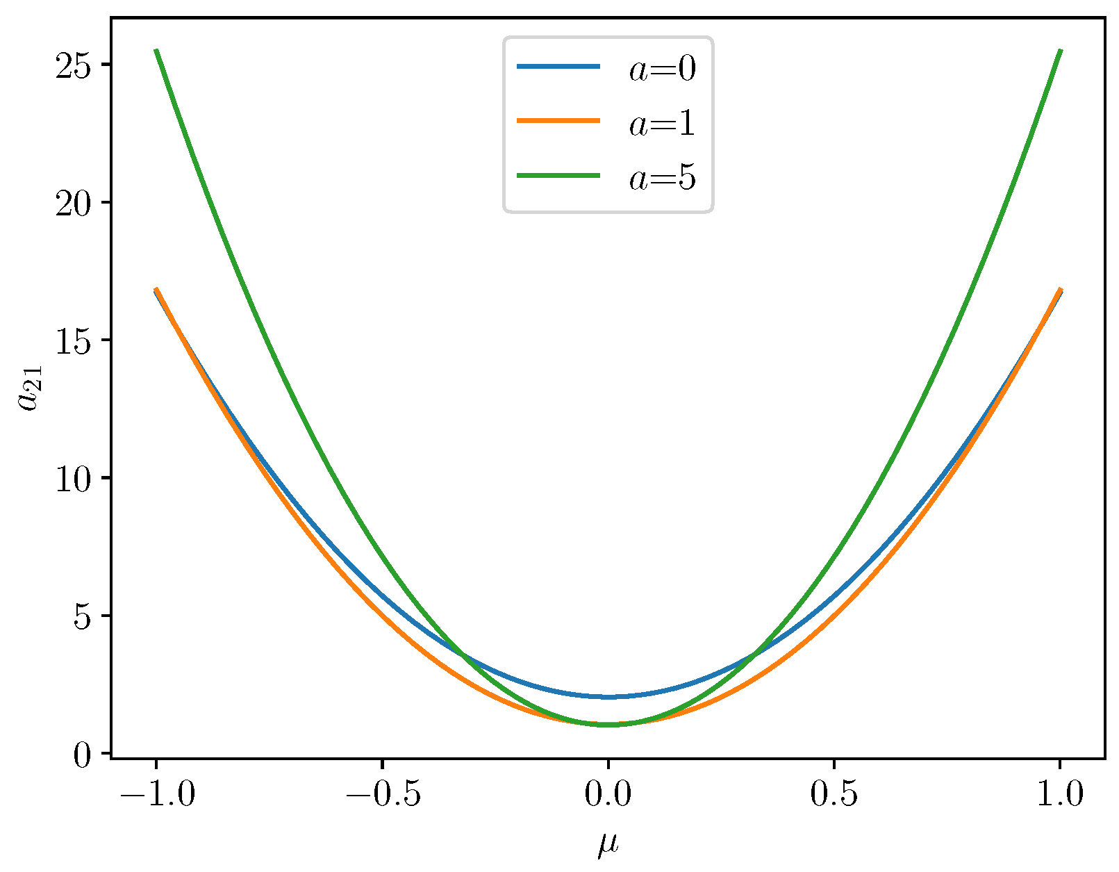
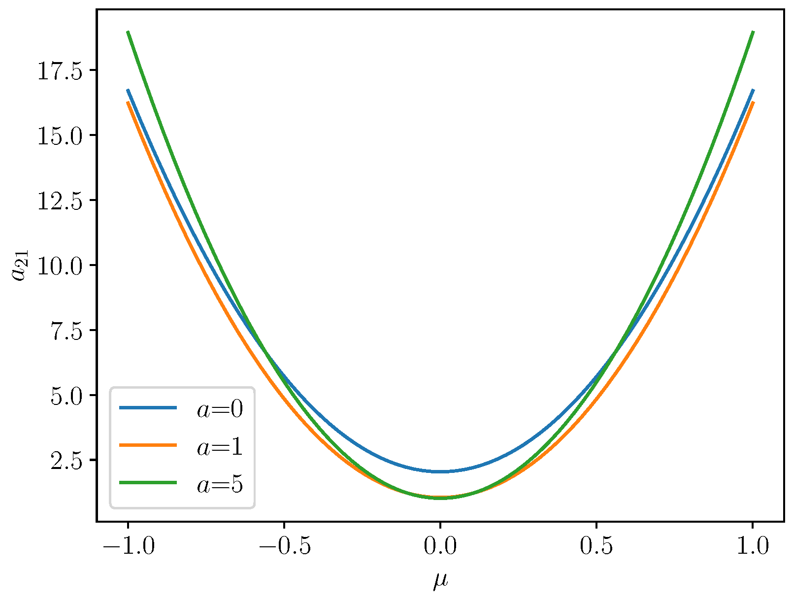
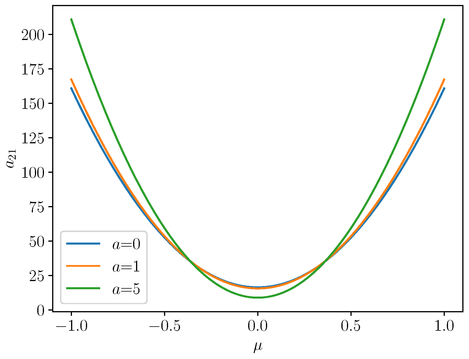
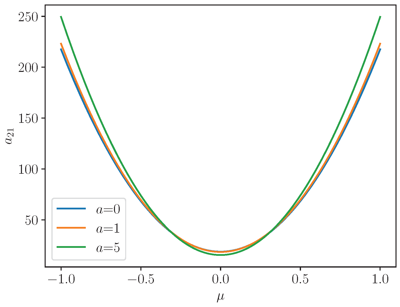
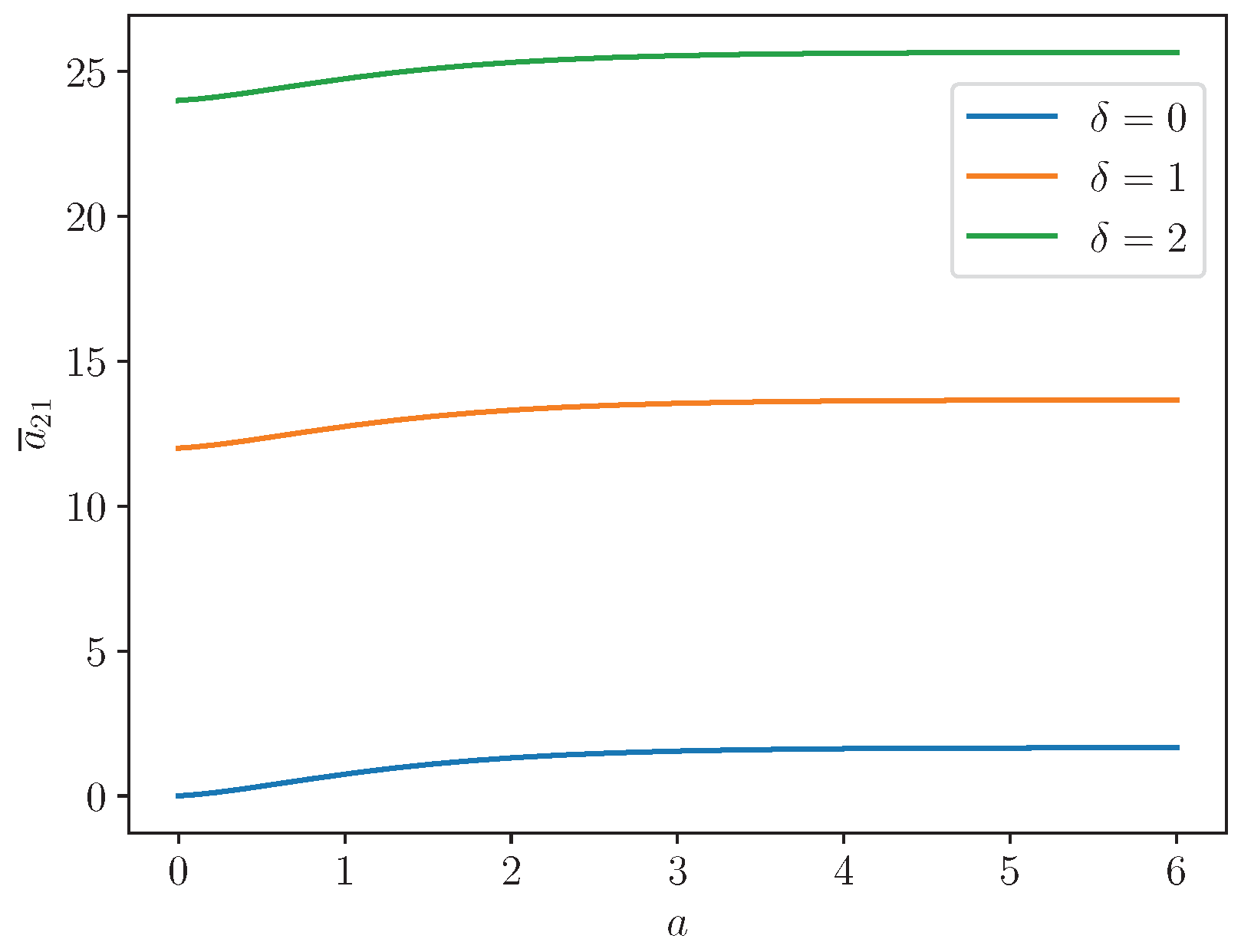
For a Gaussian process, only second-order covariances are non-zero, so that $a_{211} = {\overline{a}}_{211} = {\overline{A}}_1 = {\overline{A}}_2 = 0$. Figure 1, Figure 2, Figure 3 and Figure 4 plot $a_{21}$ for ${\gamma }_a$ against $\mu$ for a Gaussian process with ${\gamma }_T=r^{\left|T\right|}$, for lags $a=0$ (the bottom curves), $a=1,$ and $a=5$, (the top curves). The four figures are for $r=0.1$ and $r=0.9$ and for $n=10$ and $n=20$.

Note how $a_{21}$ increases rapidly with $\left|\mu \right|$ and correlation r. Doubling n has minor effect.

I now give $a_{11}$ and $a_{32}$ needed for the second-order standard-type ECF expansions, that is, the expansions to $O\left(n^{-1}\right)$. By (34), (35) and (83),

$$a_{11}=-k_1^{11}=-a_{21}^k \mathrm{of} \left(80\right),$$

(88)

$$a_{32}=-8{\mu }^3{k}_2^{111}+12{\mu }^2{k}_2^{112}-6\mu k_2^{122}+k_2^{222}-6s_1^2,s_1=-2\mu k_1^{11}+k_1^{12},$$

(89)

for $k_2^{111} = a_{32}^k$ of (81), and $k_2^{222} = a_{32}^K$ of (60). This still needs $k_2^{112}$ and $k_2^{122}$. By (66) with $r = 3,N_1 = N_2 = n,N_3 = N = n - a,$

$$\begin{array}{c}\kappa (\widehat{\mu },\widehat{\mu },{\widehat{M}}_{0a})={\left(n^{2}N\right)}^{-1}(n{a}_{32}^K+a_{33}^K)={\displaystyle \sum _{j=2}^3}{n}^{-j}{k}_j^{112}, \mathrm{where}\hfill \\ k_j^{112}=(n/N)a_{3j}^K,{\delta }_{3\mathbf{T}}=max(0,T_2,T_3+a)-m_{3\mathbf{T}},\mathrm{and} \mathrm{by} (A17),\hfill \\ K(0,T_2,T_3)=\kappa (X_0,X_{T_2},X_{T_3}{X}_{T_3+a})={\gamma }_{T_2,T_3,T_3+a}\hfill \\ +{\gamma }_{T_3}{\gamma }_{-T_2+T_3+a}+{\gamma }_{T_3+a}{\gamma }_{-T_2+T_3}\hfill \\ +\mu {\gamma }_{T_2,T_3+a}+\mu {\gamma }_{T_2,T_3}.\hfill \end{array}$$

(90)

By (66) with $r = 3,N_1 = n,N_2 = N_3 = N = n - a,$

$$\kappa (\widehat{\mu },{\widehat{M}}_{0a},{\widehat{M}}_{0a})={\left(n{N}^2\right)}^{-1}(n{a}_{32}^{K_a}+a_{33}^{K_a})=\sum _{j=2}^3{n}^{-j}{k}_j^{122}, \mathrm{where}$$

$$k_j^{122}=(n/N)a_{3j}^{K_a},\mathrm{and} {\delta }_{3\mathbf{T}}=max(a,T_2,T_3)-min(0,T_2,T_3),$$

(91)

$$\mathrm{and} K_a(0,T_2,T_3)=\kappa (X_0,X_{T_2}{X}_{T_2+a},X_{T_3}{X}_{T_3+a}) \mathrm{of} (A8).$$

(92)

This has 25 terms, or eight if $X_t$ is a Gaussian process. This completes $a_{32}$ of (89). With $a_{11}$ of (88), this gives $h_1,{\overline{h}}_1,f_1,g_1$ of (8)–(13), and the standard-type ECF expansions for ${\widehat{\gamma }}_a$ to $O\left(n^{-1}\right)$. For these expansions to $O\left(n^{-3/2}\right)$, $h_2,{\overline{h}}_2,f_2,g_2$ of (14) and (15) need $a_{22}$ and $a_{43}$. By (36),

$$\begin{array}{c}{a}_{22}=\sum (a_{22j}:j=1,2,3,6),\mathrm{where}\hfill \\ a_{221}=4{\mu }^2{k}_2^{11}-4\mu k_2^{12}+k_2^{22},a_{222}=4\mu k_2^{11},a_{223}=-2k_2^{112},a_{226}=2{\left(k_1^{11}\right)}^2.\hfill \end{array}$$

By (37), $a_{43}$ is the sum of

$$\begin{array}{c}{a}_{431}=16{\mu }^4{k}_3^{1111}-32{\mu }^3{k}_3^{1112}+24{\mu }^2{k}_3^{1122}-8\mu k_3^{1222}+k_3^{2222},\hfill \\ a_{432}=-24s_1(4{\mu }^2{k}_2^{111}-4\mu k_3^{112}+k_2^{122},a_{433}=0,a_{434}=12u_1^2{k}_1^{11}=4s_1^2{k}_1^{11},\hfill \\ \mathrm{where} s_j=-2\mu k_1^{j1}+k_1^{j2},u_1=-2s_1,u_2=0.\hfill \end{array}$$

Therefore, $k_3^{ijkl}$ is needed. $k_3^{1111} = a_{43}^k$ of (82). $k_3^{2222} = a_{43}^K$ of (64) with K of (77). Set

$$\begin{array}{c}{K}_{n31}=\kappa (\widehat{\mu },\widehat{\mu },\widehat{\mu },{\widehat{M}}_{0a}),K_{n22}=\kappa (\widehat{\mu },\widehat{\mu },{\widehat{M}}_{0a},{\widehat{M}}_{0a}),K_{n13}=\kappa (\widehat{\mu },{\widehat{M}}_{0a},{\widehat{M}}_{0a},{\widehat{M}}_{0a}).\hfill \end{array}$$

By (66) with $r = 3,N_1 = N_2 = N_3 = n,N_4 = N = n - a,$

$$\begin{array}{c}{K}_{n31}=n^{-3}{N}^{-1}(n{a}_{43}^K+a_{44}^K)={\displaystyle \sum _{j=3}^4}{n}^{-j}{k}_j^{1112} \mathrm{where} k_3^{1112}=(n/N)a_{43}^K\hfill \\ \mathrm{for} K(0,T_2,T_3,T_4)=\kappa (X_0,X_{T_2},X_{T_3},X_{T_4}{X}_{T_4+a}) \mathrm{of} (A9).\hfill \end{array}$$

(93)

Therefore, $K(0,T_2,T_3,T_4) = 0$ if $X_t$ is a Gaussian process, but in general, there are nine terms. By (66) with $r = 3,N_1 = N_2 = n,N_3 = N_4 = N = n - a,$

$$\begin{array}{c}{K}_{n22}={\left(nN\right)}^{-2}(n{a}_{43}^K+a_{44}^K)={\displaystyle \sum _{j=3}^4}{n}^{-j}{k}_j^{1122}, \mathrm{where} k_3^{1122}={(n/N)}^2{a}_{43}^K\hfill \\ \mathrm{for} K(0,T_2,T_3,T_4)=\kappa (X_0,X_{T_2},X_{T_3}{X}_{T_3+a},X_{T_4}{X}_{T_4+a})\mathrm{of} (A10).\hfill \end{array}$$

(94)

By (66) with $r = 3,N_1 = n,N_2 = N_3 = N_4 = N = n - a,$

$$\begin{array}{c}{K}_{n13}={\left(n{N}^3\right)}^{-1}(n{a}_{43}^K+a_{44}^K)={\displaystyle \sum _{j=3}^4}{n}^{-j}{k}_j^{1222}, \mathrm{where} k_3^{1222}={(n/N)}^3{a}_{43}^K,\hfill \\ \mathrm{for} K(0,T_2,T_3,T_4)=\kappa (X_0,X_{T_2}{X}_{T_2+a},X_{T_3}{X}_{T_3+a},X_{T_4}{X}_{T_4+a})\mathrm{of} (A11).\hfill \end{array}$$

(95)

Software is needed for the many terms in (94) and (95). This completes $a_{43}$, giving $h_2,{\overline{h}}_2,f_2,g_2$ of (8)–(11). These now give the standard-type ECF expansions for the distribution, density and quantiles of

$$Y_n={(n/a_{21})}^{1/2}({\widehat{\gamma }}_a-{\gamma }_a)$$

to $O\left(n^{-3/2}\right)$. The mean-type and asymptotic-type ECF expansions follow from Note 3.

For the CLT for $({\widehat{\gamma }}_0,\dots ,{\widehat{\gamma }}_a)$, see Section 9.

8. Inference for the Autocorrelation with Unknown $\mathit{\mu }$

Consider the standard-type ECF expansions to $O\left(n^{-1}\right)$ for the ath sample autocorrelation, ${\widehat{\rho }}_a$. Take $p = 3$,

$$\begin{array}{c}{w}_1=\mu ,w_2=M_{00},w_3=M_{0a},\hfill \\ {\widehat{w}}_1=\overline{X},{\widehat{w}}_2=\overline{X^2},{\widehat{w}}_3={\widehat{M}}_{0a} \mathrm{of} \left(46\right),\hfill \\ {\gamma }_0=var\left(X_0\right)=w_2-w_1^2,{\gamma }_a=covar(X_0,X_a)=w_3-w_1^2,\hfill \\ {\rho }_a={\gamma }_a/{\gamma }_0=(w_3-w_1^2)/(w_2-w_1^2)=t\left(w\right),\hfill \\ {\widehat{\gamma }}_a={\widehat{M}}_{0a}-{\overline{X}}^2,{\widehat{\gamma }}_0=\overline{X^2}-{\overline{X}}^2,{\widehat{\rho }}_a={\widehat{\gamma }}_a/{\widehat{\gamma }}_0.\hfill \end{array}$$

(96)

Accordingly, $a_{21},a_{11},a_{32}$ are given by (38) and (39) with

$$\begin{array}{c}{t}_{\blacksquare 1}=2\mu ({\rho }_a-1)/{\gamma }_0,t_{\blacksquare 2}=-{\rho }_a{\gamma }_0^{-1},t_{\blacksquare 3}={\gamma }_0^{-1},\hfill \\ t_{\blacksquare 11}=2({\rho }_a-1)(1+4{\mu }^2{\gamma }_0^{-1}){\gamma }_0^{-1},t_{\blacksquare 12}=2w_1(1-2{\rho }_a){\gamma }_0^{-2},t_{\blacksquare 13}=2w_1{\gamma }_0^{-2},\hfill \\ t_{\blacksquare 22}=2{\rho }_a{\gamma }_0^{-2},t_{\blacksquare 23}=-{\gamma }_0^{-2},t_{\blacksquare 33}=0.\hfill \end{array}$$

$k_1^{11}$ and $k_2^{111}$ are $a_{21}^k$ of (80) and $a_{32}^k$ of (81). $k_1^{33}$ and $k_2^{333}$ are $a_{21}^K$ and $a_{32}^K$ of (72). $k_1^{22}$ and $k_1^{222}$ are simply $k_1^{33}$ and $k_2^{333}$ with $a=0$. $k_1^{13}$ is $k_1^{12}$ of (86), and $k_1^{12}$ is $k_1^{13}$ with $a=0$. $k_2^{113}$ is $k_2^{112}$ of (90). $k_2^{112}$ is $k_2^{113}$ with $a=0$. $k_2^{133}$ is $k_2^{122}$ of (91). $k_2^{122}$ is $k_2^{133}$ with $a=0$. $k_1^{23}$ is $k_1^{0a}$ of Example 4.6 of [5]. (This corrects the derivatives of t given in Example 4.5 of [5]).

The approximate and asymptotic variance of the sample autocorrelation. I now show for the first time how the asymptotic variance of the sample autocorrelation of a stationary process depends on its cross-cumulants up to order four.

Corollary 4.

Set ${\gamma }_0 = var\left(X_0\right),k(i_1, \cdots , i_r) = \kappa (X_{i_1}, \cdots , X_{i_r})$ and $N = n - a$. Take $K_1(0,T)$ and $K_a(0,T)$ of (A1) and (87). The approximate variance of the sample autocorrelation with lag a,${\widehat{\rho }}_a={\widehat{\gamma }}_a/{\widehat{\gamma }}_0=({\widehat{M}}_{0a}-{\overline{X}}^2)/(\overline{X^2}-{\overline{X}}^2)$ is $a_{21}/n$, where

$$\begin{array}{c}{\gamma }_0^2{a}_{21}=4{\mu }^2{(1-{\rho }_a)}^2{k}_1^{11}+{\rho }_a^2{k}_1^{22}+k_1^{33}+4\mu ({\rho }_a-{\rho }_a^2)k_1^{12}+4\mu ({\rho }_a-1)k_1^{13}-2{\rho }_a{k}_1^{23},\hfill \\ k_1^{11}=\sum _{\left|T\right|<n}{\gamma }_T,k_1^{22}=\sum _{\left|T\right|<n}[2{\gamma }_T^2+{\gamma }_{0,T,T}+\mu ({\gamma }_{0,T}+2{\gamma }_{T,T})+4{\mu }^2{\gamma }_T],\hfill \\ k_1^{33}=(n/N)\sum _{\left|T\right|<N}{K}_1(0,T),k_1^{12}=\sum _{\left|T\right|<n}[{\gamma }_{T,T}+2\mu {\gamma }_T],\hfill \\ k_1^{13}=(n/N)\sum _{-n<T<N}{K}_a(0,T),k_1^{23}=(n/N)\sum _{-n<T<N}{K}_4(0,T)for\hfill \\ K_4(0,T)=\kappa (X_0^2,X_T{X}_{T+a})={\gamma }_{0,T,T+a}+2{\gamma }_T{\gamma }_{T+a}\hfill \\ \hspace{1em}\hspace{1em}+\mu ({\gamma }_{0,T}+{\gamma }_{0,T+a}+2{\gamma }_{T,T+a})+2{\mu }^2({\gamma }_T+{\gamma }_{T+a}).\hfill \end{array}$$

Thus the asymptotic variance of ${\widehat{\rho }}_a$ is ${\overline{a}}_{21}/n$, where

$$\begin{array}{c}{\overline{a}}_{21}=[4{\mu }^2{(1-{\rho }_a)}^2{\overline{k}}_1^{11}+{\rho }_a^2{\overline{k}}_1^{22}+{\overline{k}}_1^{33}+4\mu ({\rho }_a-{\rho }_a^2){\overline{k}}_1^{12}\hfill \\ \hspace{1em}\hspace{1em}+4\mu ({\rho }_a-1){\overline{k}}_1^{13}-2{\rho }_a{\overline{k}}_1^{23}]/{\gamma }_0^2,\hfill \\ for{\overline{k}}_1^{11}=\sum _{\left|T\right|<\infty }{\gamma }_T,{\overline{k}}_1^{33}=\sum _{\left|T\right|<\infty }{K}_1(0,T),\hfill \\ {\overline{k}}_1^{22}=\sum _{\left|T\right|<\infty }[2{\gamma }_T^2+{\gamma }_{0,T,T}+\mu ({\gamma }_{0,T}+2{\gamma }_{T,T})+4{\mu }^2{\gamma }_T],\hfill \\ {\overline{k}}_1^{12}=\sum _{\left|T\right|<\infty }[2\mu {\gamma }_T+{\gamma }_{T,T}],{\overline{k}}_1^{13}=\sum _{\left|T\right|<\infty }{K}_a(0,T),{\overline{k}}_1^{23}=\sum _{\left|T\right|<\infty }{K}_4(0,T).\hfill \end{array}$$

For example, if $\left\{X_t\right\}$ is a Gaussian process with mean μ and non-centrality parameter $\delta ={\mu }^2/{\gamma }_0,$ then

$$a_{21}=4\delta {(1-{\rho }_a)}^2\sum _{\left|T\right|<n}{\rho }_T+2{\rho }_a^2\sum _{\left|T\right|<n}({\rho }_T^2+2\delta {\rho }_T)$$

$$+(n/N)\sum _{\left|T\right|<N}[{\rho }_T^2+{\rho }_{T+a}{\rho }_{T-a})+\delta (2{\rho }_T+{\rho }_{T+a}+{\rho }_{T-a})]+8({\rho }_a-{\rho }_a^2)\delta \sum _{\left|T\right|<n}{\rho }_T$$

$$+4({\rho }_a-1)\delta (n/N)\sum _{-n<T<N}({\rho }_T+{\rho }_{T+a})$$

$$-4{\rho }_a(n/N)\sum _{-n<T<N}[\delta ({\rho }_T+{\rho }_{T+a})+{\rho }_T{\rho }_{T+a}]$$

(97)

$$\to {\overline{a}}_{21}=4\delta \sum _{\left|T\right|<\infty }{\rho }_T+(1+2{\rho }_a^2)g_0-4{\rho }_a{g}_a+g_{2a}\mathit{as}n\to \infty ,$$

(98)

$$where g_a=\sum _{\left|T\right|<\infty }{\rho }_T{\rho }_{T+a}.$$

(99)

Thus, $a_{21}$ is linear in the non-centrality parameter $\delta ={\mu }^2/{\gamma }_0$.

Proof. 

Substitute $t_{\blacksquare i}$ into $a_{21}$ of (38). $K_4$ is given by identifying $(0,0,T,T+a)$ with $(1,2,3,4)$ in (A16). For a Gaussian process, only second-order $k(.)$ are non-zero, and so (97) and (98) follow from

$$\begin{array}{c}{k}_1^{22}=\sum _{\left|T\right|<n}[2{\gamma }_T^2+{\gamma }_{0,T,T}+4{\mu }^2{\gamma }_T],\hfill \\ K_1(0,T)={\gamma }_T^2+{\gamma }_{T+a}{\gamma }_{T-a}+{\mu }^2(2{\gamma }_T+{\gamma }_{T+a}+{\gamma }_{T-a}),\hfill \\ K_a(0,T)=\mu ({\gamma }_T+{\gamma }_{T+a}),\hfill \\ K_4(0,T)=2{\gamma }_T{\gamma }_{T+a}+2{\mu }^2({\gamma }_T+{\gamma }_{T+a}),\hfill \\ k_1^{13}=\mu (n/N)\sum _{-n<T<N}({\gamma }_T+{\gamma }_{T+a}),\hfill \\ k_1^{23}=2(n/N)\sum _{-n<T<N}[{\gamma }_T{\gamma }_{T+a}+{\mu }^2({\gamma }_T+{\gamma }_{T+a})],\hfill \\ {\overline{k}}_1^{22}=f_0+f_{2a},{\overline{k}}_1^{12}=2\mu {\overline{k}}_1^{11},{\overline{k}}_1^{23}=2f_a+4{\mu }^2{\overline{k}}_1^{11}, \mathrm{where} f_a=\sum _{\left|T\right|<\infty }{\gamma }_T{\gamma }_{T+a}.\hfill \end{array}$$

□

If $a = 1$, (98) simplifies to

$${\overline{a}}_{21}=4(1+2{\rho }_1)\delta +{(1-2{\rho }_1^2)}^2 \mathrm{where} 1+2{\rho }_1=\sum _{\left|T\right|<\infty }{\rho }_T\ge 0.$$

If ${\rho }_T=r^{\left|T\right|}$, where $\left|r\right|<1$, then $g_a$ of (99) and the asymptotic variance of (98) are given by

$$\begin{array}{c}{g}_0=(1+r^2)/(1-r^2),g_a=(a+g_0)r^a,{\overline{a}}_{21}=4\delta (1+r)/(1-r)+h_a,\hfill \\ \mathrm{where} h_a=g_0(1-r^{2a})-2a{r}^{2a}\to g_0 \mathrm{as} a\to \infty ;\hfill \\ \mathrm{therefore}, \mathrm{as} a\to \infty ,{\overline{a}}_{21}\to 4\delta (1+r)/(1-r)+(1+r^2)/(1-r^2).\hfill \end{array}$$

To see that $h_a \ge 0$, note that $h_a = (1 - r^2){\sum }_{i=0}^{a-1}(2i + 1)r^{2i}.$

Contrast (98) with the CLT for ${\widehat{\rho }}_a$ given in Theorems 7.2.1 and 7.2.2 of [31], under certain conditions,

$$\begin{array}{c}{n}^{1/2}({\widehat{\rho }}_a-{\rho }_a)\stackrel{\mathcal{L}}{\to }{W}_a=\sum _{k=1}^{\infty }{A}_{ka}{N}_k\sim \mathcal{N}(0,v), \mathrm{where}\hfill \\ N_1,N_2,\dots \mathrm{are} \mathrm{independent} \mathcal{N}(0,1),A_{ka}={\rho }_{k+a}+{\rho }_{k-a}-2{\rho }_a{\rho }_k,v=\sum _{k=1}^{\infty }{A}_{ka}^2.\hfill \end{array}$$

To see that these are wrong, note that they do not include the third-order $k(i_1,i_2,i_3)$ from covariance $(\overline{X},{\widehat{M}}_{0a})$ or the fourth-order $k(i_1,i_2,i_3,i_4)$ from variance $\left({\widehat{M}}_{0a}\right)$. Similarly, $\mu$ appears in more than one of the six terms in (38) but not in [31]. Figure 5 plots ${\overline{a}}_{21}$ of (98) against lag a for $\delta ={\mu }^2/{\gamma }_0$ equal to $0,1,2$.

This shows that ${\overline{a}}_{21}$ increases much more rapidly with the noncentrality parameter $\delta$ than with the lag a.

I now move on to $a_{32}$ needed for the second-order standard-type ECF expansions for ${\widehat{\rho }}_a$. $a_{32}$ of (39) also needs $k_2^{123},k_2^{223},k_2^{233}.$ Set $N = n - a$. By (66) with

$$\begin{array}{c}r=3,N_1=N_2=n,N_3=N=n-a,\mathrm{and} ({\widehat{w}}_1,{\widehat{w}}_2,{\widehat{w}}_3)\mathrm{of} \left(96\right),\hfill \\ \kappa ({\widehat{w}}_1,{\widehat{w}}_2,{\widehat{w}}_3)={\left(n^{2}N\right)}^{-1}(n{a}_{32}^K+a_{33}^K)={\displaystyle \sum _{j=2}^3}{n}^{-j}{k}_j^{123},\mathrm{where}\hfill \\ k_j^{123}=(n/N)a_{3j}^K,\mathrm{and} K(0,T_2,T_3)=\kappa (X_0,X_{T_2}^2,X_{T_3}{X}_{T_3+a})\mathrm{of} (A12),\hfill \end{array}$$

(100)

with 17 terms, or six if $X_t$ is Gaussian. This gives $k_2^{123}$. Next I give $k_2^{223}$. By (66) with

$$\begin{array}{c}r=3,N_1=N_2=n,N_3=N=n-a,\hfill \\ \kappa ({\widehat{w}}_2,{\widehat{w}}_2,{\widehat{w}}_3)={\left(n^{2}N\right)}^{-1}(n{a}_{32}^K+a_{33}^K)={\displaystyle \sum _{j=2}^3}{n}^{-j}{k}_j^{223},\mathrm{where} k_j^{223}=(n/N)a_{3j}^K,\hfill \\ \mathrm{and} K(0,T_2,T_3)=\kappa (X_0^2,X_{T_2}^2,X_{T_3}{X}_{T_3+a})\mathrm{of} (A12).\hfill \end{array}$$

(101)

$a_{32}$ also needs $k_2^{233}$. By (66) with $r = 3,N_1 = n,N_2 = N_3 = N = n - a,$

$$\begin{array}{c}\kappa ({\widehat{w}}_2,{\widehat{w}}_3,{\widehat{w}}_3)={\left(n{N}^2\right)}^{-1}(n{a}_{32}^K+a_{33}^K)={\displaystyle \sum _{j=2}^3}{n}^{-j}{k}_j^{233},\mathrm{where} k_j^{233}={(n/N)}^2{a}_{3j}^K,\hfill \\ \mathrm{and} K(0,T_2,T_3)=\kappa (X_0^2,X_{T_2}{X}_{T_2+a},X_{T_3}{X}_{T_3+a})\mathrm{of} (A13).\hfill \end{array}$$

(102)

However, its large number of terms requires software. These now give the distribution and quantiles of

$$Y_n={(n/a_{21})}^{1/2}({\widehat{\rho }}_a-{\rho }_a)$$

to $O\left(n^{-1}\right)$. To extend this to $O\left(n^{-3/2}\right)$, write out $a_{22},a_{43}$ similarly.

The mean-type and asymptotic-type ECF expansions follow from Note 3.

9. Multivariate CLTs for Sample Autocovariances and Autocorrelations

We now come to the most important example: multivariate CLTs for the estimates of autocovariances and autocorrelations. This example concerns the asymptotic normality of the sample autocovariances, $({\widehat{\gamma }}_0, \dots , {\widehat{\gamma }}_a)$, and the sample autocorrelations, $({\widehat{\rho }}_1, \dots , {\widehat{\rho }}_a)$.

Fix $a \ge 0$ and take $0 \le a_1, a_2 \le a$. For $i = 1,2,$ set $N_i = n - a_i > 0.$

I first approximate $ncovar({\widehat{\gamma }}_{a_1},{\widehat{\gamma }}_{a_2})$ as $A^{a_1{a}_2} = K_{n1}^{a_1{a}_2}$ of (26). By (68),

$$\begin{array}{c}\kappa ({\widehat{M}}_{0a_1},{\widehat{M}}_{0a_2})={\displaystyle \sum _{j=1}^2}{n}^{-j}{k}_j^{12}=n^2{\left(N_1{N}_2\right)}^{-1}{\displaystyle \sum _{j=1}^2}{n}^{-j}{a}_{2j}^K\hfill \\ =n{\left(N_1{N}_2\right)}^{-1}{\displaystyle \sum _{-N_1<T<N_2}}(1-n^{-1}\left|T\right|)K_{a_1{a}_2}(0,T),\hfill \\ \mathrm{where} K_{a_1{a}_2}(0,T)=\kappa (X_0{X}_{a_1},X_T{X}_{T+a_2})={\displaystyle \sum _{j=1}^4}{A}_j\mathrm{by} (A16),\hfill \\ \mathrm{and} A_1={\gamma }_{a_1,T,T+a_2},\hfill \\ A_2/\mu =k(a_1,T,T+a_2)+{\gamma }_{T,T+a_2}+{\gamma }_{a_1,T+a_2}+{\gamma }_{a_1,T},\hfill \\ A_3={\gamma }_T{\gamma }_{T+a_2-a_1}+{\gamma }_{T-a_1}{\gamma }_{T+a_2},\hfill \\ A_4/{\mu }^2={\gamma }_{T+a_2-a_1}+{\gamma }_{T-a_1}+{\gamma }_{T+a_2}+{\gamma }_T.\hfill \end{array}$$

(103)

For $i = 1,2,{\widehat{\gamma }}_{a_i} = t^i\left(\widehat{w}\right) = {\widehat{w}}_i - {\widehat{w}}_0^2$, where $t^i\left(w\right) = w_i - w_0^2,w_0 = \mu ,w_i = M_{0a_i}.$ Thus, for $i = 1,2$, the non-zero first derivatives are $t_{\blacksquare 0}^i = -2\mu ,t_{\blacksquare i}^i = 1,$ and by (26), for $K_a$ of (87) and for $a_1 \ge 0,a_2 \ge 0,$

$$\begin{array}{c}{A}^{a_1{a}_2}=k_1^{a_1{a}_2}-2\mu \sum _{i=1}^2{k}_1^{0a_i}+4{\mu }^2{k}_1^{00}, \mathrm{where}\hfill \\ k_1^{00}=\sum _{\left|T\right|<n}{\gamma }_T,k_1^{0a_i}=n{N}_i^{-1}\sum _{-n<T<N_i}{K}_{a_i}(0,T) \mathrm{of} \left(87\right),\hfill \\ k_1^{a_1{a}_2}=n^2{\left(N_1{N}_2\right)}^{-1}\sum _{-N_1<T<N_2}{K}_{a_1{a}_2}(0,T) \mathrm{of} \left(103\right).\hfill \end{array}$$

Thus, by (25), for $A = (A^{a_1{a}_2}:0 \le a_1,a_2 \le a)$,

$$\begin{array}{c}{n}^{1/2}{({\widehat{\gamma }}_0-{\gamma }_0,\dots ,{\widehat{\gamma }}_a-{\gamma }_a)}^{\prime }\stackrel{\mathcal{L}}{\to }{\mathcal{N}}_{a+1}(0,A)\mathrm{as} n\to \infty .\hfill \end{array}$$

(104)

One can replace A with its asymptotic limit $\overline{A} = ({\overline{A}}^{a_1{a}_2}:0 \le a_1, a_2 \le a)$, where

$$\begin{array}{c}{\overline{A}}^{a_1{a}_2}={\overline{k}}_1^{a_1{a}_2}-2\mu \sum _{i=1}^2{\overline{k}}_1^{0a_i}+4{\mu }^2{\overline{k}}_1^{00},\mathrm{with}\hfill \\ {\overline{k}}_1^{00}=\sum _{\left|T\right|\infty }{\gamma }_T,{\overline{k}}_1^{0a_i}=\sum _{\left|T\right|\infty }{K}_{a_i}(0,T)\mathrm{of} \left(87\right),\hfill \\ {\overline{k}}_1^{a_1{a}_2}=\sum _{\left|T\right|\infty }{K}_{a_1{a}_2}(0,T)\mathrm{of} \left(103\right).\hfill \end{array}$$

Theorem 8.3.3 of [37] gave a comparable result that also allowed for the fourth-order cumulant of $X_t$ when $\mu =0$; see (3.3) of [38].

Now apply (25) to $\widehat{w} = {({\widehat{\gamma }}_0, \dots , {\widehat{\gamma }}_a)}^{\prime },\widehat{\theta } = t\left(\widehat{w}\right) = {({\widehat{\rho }}_1, \dots , {\widehat{\rho }}_a)}^{\prime },w_i = {\gamma }_i,{\rho }_i = t^i\left(\widehat{w}\right) = w_i/w_0 = {\gamma }_i/{\gamma }_0$. Under these conditions, the non-zero first derivatives are $t_{\blacksquare 0}^i=-{\gamma }_0^{-1}{\rho }_i,t_{\blacksquare i}^i={\gamma }_0^{-1},$ and by (26),

$$\begin{array}{c}{n}^{1/2}{({\widehat{\rho }}_1-{\rho }_1,\dots ,{\widehat{\rho }}_a-{\rho }_a)}^{\prime }\stackrel{\mathcal{L}}{\to }{\mathcal{N}}_a(0,B)\mathrm{as} n\to \infty ,\mathrm{where}\hfill \\ {\gamma }_0^2{B}^{a_1{a}_2}={\rho }_{a_1}{\rho }_{a_2}{A}^{00}-2\sum _{i=1}^2{\rho }_{a_i}{A}^{0a_i}+A^{a_1{a}_2}, \mathrm{for} a_1\ge 1,a_2\ge 1,\hfill \\ A^{00}=\sum _{\left|T\right|<n}({\gamma }_{0TT}+2{\gamma }_T^2-2\mu {\gamma }_{TT}+2\mu {\gamma }_{0T}),\hfill \\ A^{0a}=\sum _{\left|T\right|<n}{R}_{aT}+n{N}^{-1}\sum _{-n<T<N}{S}_{aT},N=n-a,\hfill \\ R_{aT}=-2\mu K_0(0,T)+4{\mu }^2{\gamma }_T=-2\mu {\gamma }_{T,T+a}+2{\mu }^2({\gamma }_T-{\gamma }_{T+a}),\hfill \\ S_{aT}=-K_{a0}(0,T)-2\mu K_a(0,T)\hfill \\ ={\gamma }_{aTT}+2{\gamma }_T{\gamma }_{T-a}+\mu ({\gamma }_{T-a,T-a}+{\gamma }_{T,T}-2{\gamma }_{T,T+a})+2{\mu }^2({\gamma }_{T-a}-{\gamma }_{T+a}).\hfill \end{array}$$

(105)

Note how A and B depend on the second, third, and fourth-order cross-cumulants, as well as on $\mu$.

See the figures following Corollaries 3 and 4 above for special cases of $A^{aa}$ and $B^{aa}$. One can replace B with its asymptotic limit $\overline{B} = ({\overline{B}}^{a_1{a}_2}:1 \le a_1, a_2 \le a)$, where

$$\begin{array}{c}{\gamma }_0^2{\overline{B}}^{a_1{a}_2}={\rho }_{a_1}{\rho }_{a_2}{\overline{A}}^{00}-2\sum _{i=1}^2{\rho }_{a_i}{\overline{A}}^{0a_i}+{\overline{A}}^{a_1{a}_2},\mathrm{for} a_1\ge 1,a_2\ge 1,\hfill \\ {\overline{A}}^{00}=\sum _{\left|T\right|<\infty }({\gamma }_{0TT}+2{\gamma }_T^2-2\mu {\gamma }_{TT}+2\mu {\gamma }_{0T}),\hfill \\ {\overline{A}}^{0a}=\sum _{\left|T\right|<\infty }(R_{aT}+S_{aT}).\hfill \end{array}$$

This asymptotic result corrects the celebrated Bartlett’s formula, (13) of [7]. Ref. [37] and (1.2) of ref. [38] made corrections when $\mu = 0$. Ref. [38] (p. 53) recognised that Bartlett’s formula did not allow for ’higher-order cumulants’ and gave a correction for when $\mu = 0$.

Alternatively, one can use the mean-type forms of A and B.

$({\widehat{\rho }}_1, \dots , {\widehat{\rho }}_a)$, is used as a diagnostic for model development in time series; see [31].

10. The CLT for the Third Sample Cross-Cumulant

This example concerns estimating the third cross-cumulant, ${\gamma }_{a_1,a_2} = \kappa (X_0,X_{a_1},X_{a_2})$. I give the CLT for ${\widehat{\gamma }}_{a_1,a_2}.$ Take

$$\begin{array}{c}p=5,w_1=\mu ,w_2=M_{0a_1},w_3=M_{0a_2},w_4=M_{a_1{a}_2},w_5=M_{0a_1{a}_2},\hfill \\ t\left(w\right)=\kappa (X_0,X_{a_1},X_{a_2})=w_5-w_1(w_2+w_3+w_4)+2w_1^3.\hfill \\ \mathrm{So},t_{\blacksquare 1}=6w_1^2-w_2-w_3-w_4,t_{\blacksquare 2}=t_{\blacksquare 3}=t_{\blacksquare 4}=-w_1,t_{\blacksquare 5}=1.\hfill \end{array}$$

I give $a_{21}$ needed for the CLT for its estimate $t\left(\widehat{w}\right)$. $a_{21}$ is given by (28) in terms of $k_1^{a_1{a}_2},a_1,a_2 = 1, \dots , 5$. By Section 6,

$$k_1^{11}=\sum \{{\gamma }_T:\left|T\right|<n\}.$$

For $a \ge 0$, set $k_1^{22}\left(a\right) = a_{21}$ of (84). Then for $i = 2,3,$

$$\begin{array}{c}{k}_1^{ii}=k_1^{22}\left(\right|a_i\left|\right),k_1^{44}=k_1^{22}\left(\right|a_1-a_2\left|\right).\hfill \end{array}$$

Furthermore, $k_1^{55} = a_{21}$ of Example 4. However as $\mu \ne 0$, (79) now has 178 terms, or 15 for a Gaussian process. For $N = n - \left|a\right|$ and $K_a$ of (87), set

$$\begin{array}{c}{k}_1^{12}\left(a\right)=k_1^{12}=(n/N)\sum \{K_a(0,T):-n<T<N\}.\hfill \\ \mathrm{Then} k_1^{12}=k_1^{12}\left(\right|a_1\left|\right),k_1^{13}=k_1^{12}\left(\right|a_2\left|\right),k_1^{14}=k_1^{12}\left(\right|a_1-a_2\left|\right).\hfill \end{array}$$

By (66), for N of (78),

$$\begin{array}{c}{k}_1^{15}=(n/N)\sum \{K_6(0,T):-n<T<N\},\hfill \\ \mathrm{where} K_6(0,T)=\kappa (X_0,X_T{X}_{T+a_1}{X}_{T+a_2})=M_{0,T,T+a_1,T+a_2}-\mu M_{0a_1{a}_2}.\hfill \end{array}$$

$k_1^{23}=k_1^{12}$ of Section 9. $k_1^{24}$ needs $\kappa ({\widehat{M}}_{0a_1},{\widehat{M}}_{0a_2})$, a special case of

$$\begin{array}{c}\kappa ({\widehat{M}}_{0a_1},{\widehat{M}}_{a_2{a}_3})=\sum _{j=1}^2{n}^{-j}{k}_j^{24},\mathrm{where}\hfill \\ k_j^{24}=(n^2/N_2{N}_4)a_{2j}^K,N_2=n-|a_1|,N_4=n-|a_2-a_3|,\hfill \\ \mathrm{and} K(0,T)=\kappa (X_0{X}_{a_1},X_{T+a_2}{X}_{T+a_3})=\sum _{j=1}^4{A}_j\hfill \end{array}$$

(106)

by (A16) is given by identifying $(0,a_1,T+a_2,T+a_3)$ with $(1,2,3,4)$. By (66),

$$\begin{array}{c}\kappa (\widehat{\mu },{\widehat{M}}_{0a_1{a}_1})=(n/N)\sum _{-n<T<N}{K}_7(0,T),\mathrm{where}\hfill \\ N=n-max(0,a_1,a_2)+min(0,a_1,a_2),K_7(0,T)=\kappa (X_0,X_T{X}_{T+a_1}{X}_{T+a_2}),\hfill \end{array}$$

(107)

given by identifying $(0,T,T+a_1,T+a_2)$ with $(1,2,3,4)$ in (A18).

Next I obtain $k_1^{34},k_1^{35},k_1^{45}.$ $k_1^{34}$ is a special case of (106). $k_1^{35}$ is covered by $k_1^{25}$ of (107). $k_1^{45}$ is a special case of the lead coefficient in $\kappa ({\widehat{M}}_{a_1{a}_2},{\widehat{M}}_{a_3{a}_4{a}_5}).$ In this case,

$$\begin{array}{c}{k}_1^{45}=(n^2/N_1{N}_2)\sum _{-N_1<T<N_2}{K}_8(0,T),\hfill \\ \mathrm{where} N_1=max(a_1,a_2)-min(a_1,a_2),\hfill \\ N_2=max(a_3,a_4,a_5)-min(a_3,a_4,a_5),\hfill \\ \mathrm{and} K_8(0,T)=\kappa (X_{a_1}{X}_{a_2},X_{T+a_3}{X}_{T+a_4}{X}_{T+a_5}),\hfill \end{array}$$

is given by identifying $a_1,a_2,T+a_3,T+a_4,T+a_5$ with 12345 in (A20). This has 42 terms, 18 for a Gaussian process, or zero for a zero-mean Gaussian process. This completes the terms needed for $a_{21}$ and the CLT for the estimated third-order cumulant. Similarly, we can obtain the CLT for the sample cross-cumulant of degree four, $\widehat{\gamma }(a_1,a_2,a_3),$ and the CLT for $\widehat{k}(a_1,a_2,a_3)$.

Note how Section 8 built on Section 6, Section 9 built on Section 7 and Section 8, and Section 10 built on Example 4 and Section 9. Thus, the above results form a catalogue upon which other examples can build.

• Example 4 gave $a_{21}=k_1^{11}$ for ${\widehat{w}}_1={\widehat{M}}_{0a_1{a}_2}.$
• Section 6 gave $a_{21}=k_1^{11},a_{32}=k_2^{111},a_{22}=k_2^{11},a_{43}=k_3^{1111}$ for $\overline{X}$.
• Section 7 gave $k_1^{ij},k_2^{ijk}$ for ${\widehat{w}}_1=\overline{X},{\widehat{w}}_2={\widehat{M}}_{0a}$ needed for the distribution of ${\widehat{\gamma }}_a$.
• Section 8 gave $k_1^{ij},k_2^{ijk}$ for ${\widehat{w}}_1=\overline{X},{\widehat{w}}_2=\overline{X^2},{\widehat{w}}_3={\widehat{M}}_{0a}$.
• Section 9 gave $k_1^{ij}$ for ${\widehat{w}}_0=\overline{X},{\widehat{w}}_1={\widehat{M}}_{0a_1},{\widehat{w}}_2={\widehat{M}}_{0a_2}$.
• Section 10 gave $a_{21}=k_1^{11}$ for ${\gamma }_{a_1,a_2}=\kappa (X_0,X_{a_1},X_{a_2})$.

Note 4.

Set $Y_t = X_t - \mu$. By Holder’s inequality, for $r \ge 2,$

$$\begin{array}{c}|\mu (X_{t_1},\dots ,X_{t_r})|=|E{Y}_{t_1}\dots Y_{t_r}|\le E|Y_0{|}^r=E{|X_0-\mu |}^r.\hfill \end{array}$$

I call

$${\rho }_{t_1,\dots ,t_r}=\mu (X_{t_1},\dots ,X_{t_r})/E{|X_0-\mu |}^r,$$

the autocorrelation of degree r, since it lies in $[-1, 1]$. I have not found this concept in the literature, apart from the usual case $r = 2$. For $r = 2, 4, 6, \dots$, the methods here can be applied to give a CLT for ${\widehat{\rho }}_{t_1,\dots ,t_r}$. For $r = 3, 5, \dots$, ${\widehat{\rho }}_{t_1,\dots ,t_r}$ satisfies an interesting CLT, but I shall not give details here.

11. Multivariate Stationary Processes

Section 3 spelt out how to obtain the distribution of any smooth function $t\left(\widehat{w}\right):R^p\to R^q$ of a standard estimate $\widehat{w}$ to $O\left(n^{-3/2}\right)$. The examples were all based on univariate stationary $X_t$.

Now suppose that $\cdots ,X_{-1},X_0,X_1,\cdots$ lie in $R^p$ and are stationary with finite moments. For $j = 1, \cdots , p$, denote the jth component of $X_t$ as $X_t^j$ and the mean, cross-moments, and cross-cumulants as

$$\begin{array}{c}\mu =E{X}_0,{\mu }^j=E{X}_0^j,M_{t_1\cdots t_r}^{j_1\cdots j_r}=E{X}_{t_1}^{j_1}\cdots X_{t_r}^{j_r},\hfill \\ {\mu }_{t_1\cdots t_r}^{j_1\cdots j_r}=E(X_{t_1}^{j_1}-{\mu }^{j_1})\cdots (X_{t_r}^{j_r}-{\mu }^{j_r}),k\left({\displaystyle \genfrac{}{}{0pt}{}{j_1\cdots j_r}{t_1,\cdots ,t_r}}\right)=\kappa (X_{t_1}^{j_1},\cdots ,X_{t_r}^{j_r}).\hfill \end{array}$$

(108)

Given a sequence of integers $t_1,\cdots ,t_r$, define $t_0,I_k$ as in (42). Then, (43) becomes

$$\begin{array}{c}\hfill M_{t_1\cdots t_r}^{j_1\cdots j_r}=M_{I_1\cdots I_r}^{j_1\cdots j_r},{\mu }_{t_1\cdots t_r}^{j_1\cdots j_r}={\mu }_{I_1\cdots I_r}^{j_1\cdots j_r},k\left({\displaystyle \genfrac{}{}{0pt}{}{j_1\cdots j_r}{t_1\cdots t_r}}\right)=k\left({\displaystyle \genfrac{}{}{0pt}{}{j_1\cdots j_r}{I_1\cdots I_r}}\right).\end{array}$$

However, in general, $k\left({\displaystyle \genfrac{}{}{0pt}{}{j_1{j}_2}{0,I}}\right)\ne k\left({\displaystyle \genfrac{}{}{0pt}{}{j_1{j}_2}{0,-I}}\right)$. An unbiased estimator of $M\left({\displaystyle \genfrac{}{}{0pt}{}{j_1\cdots j_r}{t_1\cdots t_r}}\right)$ is

$$\begin{array}{c}\hfill {\widehat{M}}_{t_1\cdots t_r}^{j_1\cdots j_r}=N^{-1}\sum _{t=1}^N{X}_{t+I_1}^{j_1}\cdots X_{t+I_r}^{j_r}\mathrm{for} N=n-I_0>0.\end{array}$$

One can abbreviate two sequences of integers of the same length r as $\pi = (t_1\cdots t_r),\tau = (j_1\cdots j_r).$ Given $P \ge 1$ and finite sequences of integers ${\pi }_1, \cdots , {\pi }_P$ and ${\tau }_1, \cdots , {\tau }_P$ not depending on n with ${\tau }_i$ of the same length as ${\pi }_i$,

$$\begin{array}{c}\mathrm{set} w_a=M_{{\pi }_a}^{{\tau }_a},{\widehat{w}}_a={\widehat{M}}_{{\pi }_a}^{{\tau }_a},w=(w_1,\cdots ,w_p),\widehat{w}=({\widehat{w}}_1,\cdots ,{\widehat{w}}_p).\hfill \\ \mathrm{Then} \kappa ({\widehat{w}}_{a_1},\cdots ,{\widehat{w}}_{a_r})=\sum _{j=r-1}^r{n}^{-j}{k}_j^{a_1\cdots a_r}for{a}_1,\cdots ,a_r\in \{1,\cdots ,p\}.\hfill \end{array}$$

Let $\theta =t\left(w\right):R^p\to R^q$ be a function with finite derivatives (23) at $w=E{X}_0$. Then $\widehat{\theta }=t\left(\widehat{w}\right)$ satisfies (24), and $Y_n=n^{1/2}(\widehat{w}-w)$ and $Z_n=n^{1/2}(\widehat{\theta }-\theta )$ have multivariate Edgeworth expansions. The results of Section 4 apply when each $K(t_1\dots t_r)$ is replaced with its extension $K\left({\displaystyle \genfrac{}{}{0pt}{}{j_1\cdots j_r}{t_1\cdots t_r}}\right)$ and $K\left({\displaystyle \genfrac{}{}{0pt}{}{{\pi }_1\dots {\pi }_r}{t_1\dots t_r}}\right)$ of (50) is replaced with its extension.

Example 5.

This example concerns ECF expansions for the multivariate sample mean, $\widehat{w}=\widehat{\mu }=\overline{X}$ of (45), to $O\left(n^{-3/2}\right)$.

Take $p \ge 1,\pi = \left(0\right)$ so that ${\widehat{M}}_0 = \widehat{\mu } = \overline{X}$. For $r \ge 2$ and $K(.) = k(.)$ of (41),

$$\begin{array}{c}{\kappa }^{1\dots r}\left(\overline{X}\right)=n^{1-r}{a}_{r,r-1}^k+n^{-r}{a}_{rr}^k of \left(\mathsf{70}\right) with N=n,\hfill \\ \kappa \left({\displaystyle \genfrac{}{}{0pt}{}{{\pi }_1\cdots {\pi }_r}{0,T_2,\cdots ,T_r}}\right)=k\left({\displaystyle \genfrac{}{}{0pt}{}{j_1\cdots j_r}{0,T_2,\cdots ,T_r}}\right) of \left(\mathsf{108}\right)=\kappa (X_0^{j_1},X_{T_2}^{j_2},\dots ,X_{T_r}^{j_r}).\hfill \end{array}$$

This example was the subject of [4,5].

12. Discussion

The CLT (2) for $\overline{X}$, the mean of a sample from a stationary process, is well known. However, not until very recently, in [4], were its ECF expansions given. CLTs for the sample autocorrelation, ${\widehat{\rho }}_a$, and for $({\widehat{\rho }}_1,\dots ,{\widehat{\rho }}_a)$ were given in [31]. However these did not allow for the first-, third- or fourth-order cross-cumulants. I corrected these shortcomings in Section 8 and Section 9. Section 8 also gives the ECF expansions of ${\widehat{\rho }}_a$ to $O\left(n^{-3/2}\right)$, and explains how to improve this to $O\left(n^{-2}\right)$, as well as how to extend it to the distribution of $({\widehat{\rho }}_1,\dots ,{\widehat{\rho }}_a)$.

Empirical distribution functions, kernel density estimation, and resampling techniques such as bootstrapping are all actively used in the analysis of stationary processes. However, while these are nonparametric techniques, unlike the content of this paper, they do not provide the nonparametric theory for the distribution of the general standard estimator based on a sample from a stationary process, given here. Consequently, econometrics, the foremost user of time series, has been dominated by software constructing and applying estimators for parametric ARMA processes and the like. However, as noted, parametric models suffer from a severe drawback: if the model is wrong, the results will generally not even give first-order (CLT) accuracy. This is where a nonparametric method is superior. Furthermore, the Kalman filter and prediction in ARMA time series with their Wold and Kolmogorov representations assume that $\mu =0$; see 8.6 and 10.9 of [39]. We are less interested in this case, although it is important because it is used frequently in radio, radar, controls and communications work; see [40] and 1.2 of [41]. In this case, the terms with $\mu$ in Corollaries 3 and 4 and, more generally, in Appendix B are zero.

Software is not needed for third-order ECF expansions for the sample mean, $\overline{X}$, the sample autocovariance, ${\widehat{\gamma }}_a$, or the CLT for the sample autocorrelations. However, software is needed for the second-order ECF expansions for the sample autocorrelations because of the large numbers of terms for the K functions. Software is also needed in Example 4 and Section 10 when computing the asymptotic variance of the estimates of third-order cross-moments and cross-cumulants.

However in many areas of signal detection, including radio, radar, sonar, speech, image analysis, communications, control and seismology, the time series can often be assumed to be Gaussian; see, for example, [39,40,42]. In this important case, many of the terms in Appendix B are zero; see, for example, Corollaries 3 and 4.

Future directions.

1. The CLTs for ${\widehat{\gamma }}_a$ and ${\widehat{\rho }}_a$ in Section 7 and Section 8 and the CLTs of $({\widehat{\gamma }}_1,\dots ,{\widehat{\gamma }}_a)$ and $({\widehat{\rho }}_1,\dots ,{\widehat{\rho }}_a)$ in (104) and (105) have many applications, as Bartlett’s formula generally ignores the effect of non-zero mean and higher cross-cumulants.

2. I included only one example in Section 11 for multivariate stationary series, as it deserves its own paper.

3. Section 9 gives CLTs for $({\widehat{\gamma }}_0,\dots ,{\widehat{\gamma }}_a)$ and $({\widehat{\rho }}_1,\dots ,{\widehat{\rho }}_a)$. These can be used for model development in time series, as in [31]. Extending Section 9 to Edgeworth expansions of order two or three for $({\widehat{\rho }}_1,\dots ,{\widehat{\rho }}_a)$, that is, to $O\left(n^{-1}\right)$ or $O\left(n^{-3/2}\right)$, will require software.

4. Extensions to signal plus noise problems, to partial autocorrelation, and to autocorrelation in regression are needed.See [27,43] and Chapter VII of [44].

5. These results can easily be extended to both weighted estimators and estimators based on series with missing data, as performed in [4].

6. Ref. [45] gave $a_{21}$ and a CLT for weighted sums of a spatial process. It should be feasible to extend this to give the other leading $a_{rj}$. A CLT for the spatial autocorrelation would also be useful. See [46,47,48].

7. To extend these results to confidence intervals for a general function of cross-cumulants, say, $t\left(w\right)$, would be an important advancement. The first step is to extend them to Edgeworth expansions for the studentized form

$$(t\left(\widehat{w}\right)-t\left(w\right))/{\widehat{a}}_{21}^{1/2}, \mathrm{where} {\widehat{a}}_{21}=\sum \{\widehat{K}(0,T):\left|T\right|<l_n\}$$

is a consistent estimator of $a_{21}$ of (59), and one can take $l_n = L{n}^{1/2}$ for some $L > 0$. Ref. [49] gave this to $o\left(n^{-1}\right)$ for the case $t\left(w\right) = \mu$, so that $K(0,T) = \kappa (X_0,X_T)$, using ${\widehat{M}}_{0T}$ of Section 7.

8. Similarly, one could estimate $a_{32}^k$ of (81) with

$${\widehat{a}}_{32}^k=\sum [{\widehat{\gamma }}_{T_2,T_3}:|T_j|<L{n}^{1/2},j=2,3]$$

for ${\widehat{\gamma }}_{T_2,T_3}$ of Section 10. Other $a_{ri}^K$ can be estimated similarly.

9. How sensitive are the results to the estimation of the many higher-order cross-cumulants required? A numerical study to consider this for some examples would be useful.

10. Software to implement the results of Section 3 for any smooth function of w would be useful.

11. Software to extend the results of [1] and to spell out its succinct notation as shown in the Appendix A below would be useful. For example, results from [1] allowed me to obtain $a_{43}$ for ${\kappa }_4\left({\widehat{M}}_{i_1{i}_2}\right)$ but not $a_{32}$ for ${\kappa }_3\left({\widehat{M}}_{i_1{i}_2{i}_3}\right)$.

12. One could replace my empirical estimator of the cross-cumulant with a less biased estimator. While a jack-knife or bootstrap could be used, analytic results are more easily obtained by adjusting it with an estimator of its bias. However, its advantage is limited, as this may only remove the first term in $a_{22}$ of (30).

13. There is also the prospect of tilted extensions. These extend the applicability of univariate Edgeworth expansions to the whole line; see [16].