Command-Filtered Fuzzy Adaptive Output Feedback Control for Nonlinear Power Systems with Actuator Faults

Abstract

This study presents a command-filtered fuzzy adaptive control method for nonlinear thyristor controlled series compensation (TCSC) systems subject to actuator faults, unknown nonlinearities, and unmeasurable states. To enhance applicability, the TCSC-based single-machine infinite-bus (SMIB) system is first transformed into a nonlinear form preserving the inherent nonlinear characteristics of the power system. A state observer is then designed to estimate the unmeasurable states. Using these estimated states, a fuzzy control algorithm approximates the uncertain nonlinearities. By integrating command filtering techniques, an adaptive output feedback controller is developed, which ensures system stability and avoids the “explosion of complexity” issue. Simulation results verify the effectiveness of the proposed control approach.

1. Introduction

Due to the increasing demand for electrical energy and the need for enhanced power standards, there has been a substantial expansion and rapid development of power systems. It is imperative to address the stability of modern power systems, whose growing complexity makes this an issue that cannot be overlooked [1,2]. As a member of the flexible alternative current transmission system (FACTS) family, they have the function of enhancing the transmission capacity of high-voltage long-distance power lines, improving system stability, damping sub-synchronous and low-frequency oscillations, and continuously regulating and controlling power flows [3]. Among the control methods for TCSC, linear control is one of the most commonly used [4,5,6]. However, linear control methods suffer from several problems, such as low control accuracy and moderate response speed. To overcome these problems, a growing number of scholars have begun to focus on the application of nonlinear control methods to TCSC.

Output feedback control, a widely used nonlinear control technique, involves utilizing available output information to design feedback controllers that can effectively regulate the system state. In the past few years, there has been significant progress in the advancement of nonlinear output feedback control techniques by scholars [7,8,9,10,11]. Ref. [12] proposed an adaptive fuzzy finite time command filter control scheme to handle nonlinear issues. The research presented in [13] introduced dynamic surface control (DSC) technology as a solution to the issue of “complexity explosion” encountered in conventional backstepping control methods [14,15,16], distinguishing it from previous studies on adaptive output feedback control. In [17], a control method was proposed that integrated a nonlinear adaptive control algorithm based on state feedback with observer-based adaptive output feedback, effectively mitigating the performance degradation caused by state feedback.

However, the aforementioned research on output feedback control methods has not taken into account the occurrence of faults, while in practice, actuator failures are inevitable during the long-term operation of real power systems. Therefore, studying TCSC-equipped systems under output feedback in the presence of faults holds significant value and research importance.

Actuator failures, which are unavoidable in modern dynamic systems, can degrade performance or cause instability [18,19,20], highlighting the need for effective fault-tolerant strategies [21,22,23]. Significant research has addressed actuator faults in various systems [24,25,26]; for example, a fuzzy-enhanced adaptive containment control method is developed in [27] for nonlinear multi-agent systems with delay and actuator faults. A key limitation of existing approaches is their assumption of known control coefficient signs, a condition often unmet in practice where control directions may be unknown. This has spurred recent interest in unknown control direction problems. Representative studies include [28] on tunnel prescribed control under unknown directions, ref. [29] on tracking control with state constraints and direction uncertainty, and [30] on fixed-time synchronization based on the Takagi–Sugeno model. Adaptive fault-tolerant tracking under unknown directions is examined in [31], and fuzzy-based tracking control for multi-agent systems with actuator faults and unknown directions is addressed in [32].

Therefore, this study proposes an adaptive fault-tolerant control method for a class of uncertain nonlinear systems that can be applied to an SMIB system with TCSC. The main findings of this investigation are summarized as follows:

1.

The paper presents a command filter control approach for power systems incorporating uncertain nonlinear components with TCSC. In contrast to the control methods discussed in previous studies [5,6], which treated nonlinear dynamical systems as linear ones, our proposed control scheme demonstrates enhanced practicality.

2.

Compared with the traditional dynamic surface control technique used in [13], the command filter employed in this paper demonstrates superior control performance when handling such nonlinear systems with actuator faults. It results in a smaller overall system tracking error, enables faster convergence to a small neighborhood around zero, and provides better control accuracy.

3.

The control method based on FLSs adopted in this paper relaxes the linear growth condition of nonlinear terms in the system compared with [33,34] and can be applied in a broader range of scenarios.

The structure of this article is as follows: System analysis and modeling are provided in Section 2. Section 3 details the primary results regarding the design of the output feedback controller and the accompanying stability analysis of the system. The simulation of an SMIB system with TCSC is included in Section 4. Finally, the conclusion is given in Section 5.

2. SystemAnalysis and Modeling

2.1. Description of the System

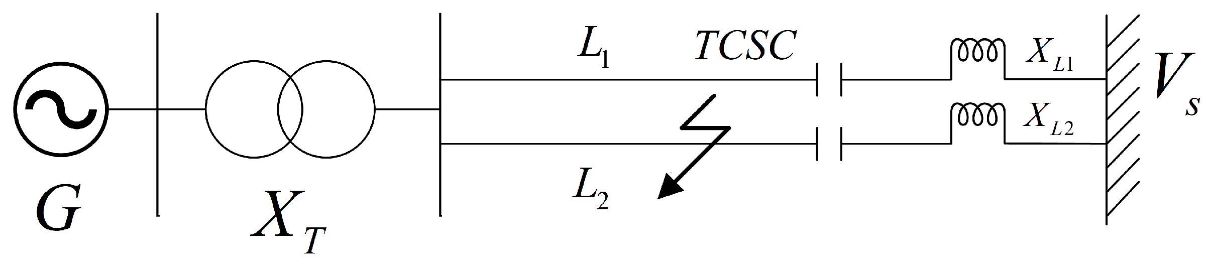
Consider an SMIB system with TCSC [35,36], which is mainly composed of a generator, transformer, transmission line and TCSC. The specific system model is shown in Figure 1.

Where G denotes the generator; $X_T$ is the leakage reactance of the transformers; $L_1$ and $L_2$ are the transmission lines, with $X_{L1}$ and $X_{L2}$ representing their respective reactance; and $V_s$ is the voltage of the infinite bus.

Figure 1. Configuration of an SMIB system with TCSC.

Figure 1. Configuration of an SMIB system with TCSC.

If we disregard the electromagnetic transient phenomena occurring in both the transmission line and the TCSC itself and assume that the generator can be represented by a constant voltage source connected through a transient reactance, then we can mathematically represent the SMIB system with TCSC using the subsequent nonlinear equation:

$$\left\{\begin{array}{c}\dot{\delta }=\omega -{\omega }_0\hfill \\ \dot{\omega }=-{\displaystyle \frac{D}{H}}\left(\omega -{\omega }_0\right)+{\displaystyle \frac{{\omega }_0}{H}}\left(P_m-{\displaystyle \frac{E_q^{\prime }{V}_s\sin \delta }{X_{d\Sigma }^{\prime }+X_{\mathrm{tcsc}}}}\right)\hfill \end{array}\right.$$

(1)

where $\delta$ represents the generator rotor angle, indicating its rotational position; $\omega$ denotes the rotor speed of the generator; $P_m$ signifies the mechanical power output of the prime mover; H refers to the moment of inertia of the dynamo’s rotor; and D and $E_q^{\prime }$ represent coefficients related to damping effects and instantaneous potential along the q-axis of the generator. $X_{d\Sigma }^{\prime }=X_d^{\prime }+X_T+X_L$ indicates external reactance, $X_d^{\prime }$ represents transient reactance along the d-axis for this specific generator model, and $X_L$ stands for transmission line reactance. $X_{tcsc}$ is the control variable and represents the equivalent reactance of TCSC. $\left({\delta }_0,{\omega }_0\right)$ is the steady-state operating point of a certain selected generator.

If the state variable dimensions are defined as $x_1=\delta -{\delta }_0$, $x_2=\omega -{\omega }_0$, and we choose the control variable as $u=1/\left(X_{d\Sigma }^{\prime }+X_{\mathrm{tcsc}}\right)$, then the system (1) is transformed as:

$$\left\{\begin{array}{c}{\dot{x}}_1=x_2\hfill \\ {\dot{x}}_2=a_0+q_1{x}_2+q_2\sin \left({\delta }_0+x_1\right)u^f\hfill \end{array}\right.$$

(2)

where $a_0=P_m{\displaystyle \frac{{\omega }_0}{H}}$, $q_1=-{\displaystyle \frac{D}{H}}$, and $q_2=-{\displaystyle \frac{{\omega }_0{E}_q^{\prime }{V}_s}{H}}$.

Remark 1.

In practical engineering, the damping coefficient D is difficult to measure accurately under normal circumstances, so it inevitably contains certain uncertainties. The parameter D is assumed to have an uncertain value, thereby implying that the parameter $q_1$ also possesses uncertainty in its value.

Let $g_2=q_2\sin \left({\delta }_0+x_1\right)$, $f_2=a_0+q_1{x}_2$, and consider the influence of disturbances, where $g(·)$ is a known smooth function satisfying $g(·)\ne 0$ and $\left|g(·)\right|\le \overline{g}$, with $\overline{g}$ being a positive constant; $d_1$ and $d_2$ are unknown external system disturbances. This can be further generalized to the following expression:

$$\left\{\begin{array}{c}{\dot{x}}_1=x_2+f_1\left({\overline{x}}_1\right)+d_1\left(t\right)\hfill \\ {\dot{x}}_2=g_2\left({\overline{x}}_2\right)u^f+f_2\left({\overline{x}}_2\right)+d_2\left(t\right)\hfill \\ y=x_1\hfill \end{array}\right.$$

(3)

Among them, ${\overline{x}}_1=x_1^T\in R$, ${\overline{x}}_2={\left[x_1,x_2\right]}^T\in R^2$, and $u^f\in R$ represent the system state vector and control input, respectively; $f_1\left(x\right)$ and $f_2\left(x\right)$ are unknown smooth nonlinear functions; $g_2\left(\overline{x}\right)$ denotes a known smooth bounded continuous function, satisfying $g(·)\ne 0$ and $\left|g(·)\right|\le \overline{g}$; and $d\left(t\right)$ is an unknown external system disturbance satisfying $\overline{d}>0$ and $\left|d\left(t\right)\right|\le \overline{d}$, and only the output $y=x_1$ is measurable.

The actuator fault types considered in this paper are as follows:

$$u^f\left(t\right)=\rho v\left(t\right)+\gamma \left(t\right)$$

Assumption 1

([37]). This work considers an actuator fault model characterized by two elements: 1. An uncertain effective factor ρ bounded by a known positive constant $\overline{\rho }(\left|\rho \right|\le \overline{\rho })$. 2. An unknown time-varying function $\gamma \left(t\right)$ with an upper bound $\overline{\gamma }(\left|\gamma \left(t\right)\right|\le \overline{\gamma })$. Critically, to mitigate the risk of controller failure induced by jamming faults, the bound $\overline{\rho }$ is strictly confined to the operational range of $\left(0, 1\right]$.

Assumption 2.

For $\forall X_1,X_2\in R^i$, there exist $h_i$ (where $h_i$ represent a series of constants and $i=1,\dots ,n$) such that the following inequality holds:

$$|f_i\left(X_1\right)-f_i\left(X_2\right)|\le h_i\parallel X_1-X_2\parallel$$

where $\parallel X_1-X_2\parallel$ denotes the 2-norm of the vector $X_1-X_2$.

Remark 2.

The practical validity of the actuator fault model assumptions is demonstrated by physical constraints. The effective factor ρ possesses a lower bound as an excessively small value would render the actuator inoperative and the controller useless. Concurrently, the magnitude of $\gamma \left(t\right)$ is naturally restricted by the actuator’s physical capabilities. Hence, the boundedness assumption is justified.

Remark 3.

The control objective of this paper is to design a fault-tolerant controller that can ensure system stability even in the event of actuator faults. Common types of actuator faults can be classified into partial failure faults (damage faults, drift faults) and complete failure faults (lock-in-place faults, saturation faults). This paper primarily considers the scenario of partial failure faults, including damage faults and drift faults. However, to ensure the controllability of the controller, complete failure faults are not considered in this study, as an effectiveness factor $\rho =0$ would render the designed controller $v\left(t\right)$ completely ineffective for system control.

2.2. Description of Fuzzy Logic Systems

For uncertain nonlinear terms in nonlinear systems, fuzzy logic systems (FLSs) are often employed for approximation and handling. A fuzzy logic system consists of several distinct components. The fuzzy dynamics of the system can be described by a set of k fuzzy IF–THEN rules, which form the core of the fuzzy inference process. The j-th rule $R^j(j=1,\dots ,k)$ is defined as:

$R^j$: If $a_1$ is $K_1^j$, ⋯ and $a_n$ is $K_n^j$, then $y\left(a\right)$ is $L^j$. Here, $a={\left[a_1,\dots ,a_n\right]}^T\in R^n$ is the state vector of the system and $y\in R$ is the output. The terms $K_m^j(m=1,\dots ,n)$ and $L^j$ are linguistic values represented by fuzzy sets, with ${\mu }_{K_m^j}\left(a\right)$ and ${\mu }_{L^j}\left(y\right)$ being their corresponding membership functions that quantify the degree of membership. The fuzzy dynamics system is constructed according to the following definition:

$$y\left(a\right)={\displaystyle \frac{{\sum }_{j=1}^k{W}_j{\prod }_{j=1}^n{\mu }_{K_m^j}\left(a_j\right)}{{\sum }_{j=1}^k\left[{\prod }_{j=1}^n{\mu }_{K_m^j}\left(a_j\right)\right]}}$$

(4)

where $W_j={\max }_{y\in R}{\mu }_{L^j}\left(y\right)$. We define two variables $S\left(a\right)={\left[S_1\left(a\right),S_2\left(a\right),\dots ,S_k\left(a\right)\right]}^T$ and $W={\left[W_1,\dots ,W_k\right]}^T$. We then define function $S_j\left(a\right)={\displaystyle \frac{{\prod }_{j=1}^n{\mu }_{K_m^j}\left(a_j\right)}{{\sum }_{j=1}^k\left[{\prod }_{j=1}^n{\mu }_{K_m^j}\left(a_j\right)\right]}}$, and FLSs can be expressed as

$$y\left(a\right)=W^{T}S\left(a\right)$$

(5)

Lemma 1

([37]). Given a continuous function $f\left(z\right)\in \mathsf{\Omega }$, a fuzzy logic system can be constructed to satisfy the inequality below, in which ε denotes a positive constant:

$$\underset{z\in \mathsf{\Omega }}{\sup }\left|f\left(z\right)-W^{T}S\left(z\right)\right|\le \epsilon$$

Lemma 2

([38]). For any $\left(x,y\right)\in R^2$, there exists the following inequality constraints:

$$xy\le {\displaystyle \frac{x^{a_s}}{a_s}}+{\displaystyle \frac{y^{b_s}}{b_s}}$$

where $a_s>1$, $b_s>1$, $\left(1/\phantom{1a}{a}_s\right)+\left(1/\phantom{1b}{b}_s\right)=1$.

Lemma 3

([39]). The command filter is defined according to the following expression:

$$\left\{\begin{array}{c}{\dot{\phi }}_1={\omega }_p{\phi }_2\hfill \\ {\dot{\phi }}_2=-2m_1{\omega }_p{\phi }_2-{\omega }_p\left({\phi }_1-{\alpha }_1\right)\hfill \end{array}\right.$$

with initial conditions ${\phi }_1\left(0\right)={\alpha }_1\left(0\right)$ and ${\phi }_2\left(0\right)=0$, supposing that $\left|{\dot{\alpha }}_1\right|\le o_1$ and $\left|{\ddot{\alpha }}_1\right|\le o_2$, where $o_1>0$ and $o_2>0$. For any $\xi >0$, if ${\omega }_p>0$ and $m_1\in \left(0,1\right]$ such that $\left|{\phi }_1-{\alpha }_1\right|\le \xi$, $\left|{\dot{\phi }}_1\right|$, $\left|{\ddot{\phi }}_1\right|$, and $\left|{\stackrel{⃛}{\phi }}_1\right|$ are bounded.

2.3. Fuzzy State Observer Design

For system (3), one has:

$$X_i=x_i/\rho ,i=1,2$$

(6)

Then the above system can be expressed as:

$$\left\{\begin{array}{c}{\dot{X}}_1=F_1\left({\overline{X}}_1\right)+X_2+D_1\left(t\right)\hfill \\ {\dot{X}}_2=F_2\left({\overline{X}}_2\right)+G_2\left({\overline{X}}_2\right)\left[v\left(t\right)+{\displaystyle \frac{\gamma \left(t\right)}{\rho }}\right]+D_2\left(t\right)\hfill \\ Y=X_1\hfill \end{array}\right.$$

(7)

where $F_i\left({\overline{X}}_i\right)=f_i\left({\overline{x}}_i\right)/\rho$, $D_i\left(t\right)=d_i\left(t\right)/\rho$, and ${\overline{X}}_i={\left[x_1/\rho ,x_2/\rho \right]}^T\in R^2$ for $i=1,2$, and $G_2\left({\overline{X}}_2\right)=g_2\left({\overline{x}}_2\right)/\rho$.

Then, we rewrite the above system (7) as follows:

$$\left\{\begin{array}{c}{\dot{X}}_1=F_1\left({\overline{X}}_1\right)+X_2+D_1\left(t\right)\hfill \\ {\dot{X}}_2=F_2\left({\widehat{\overline{X}}}_2\right)+\Delta F_2+G_2\left({\overline{X}}_2\right)\left[v\left(t\right)+{\displaystyle \frac{\gamma \left(t\right)}{\rho }}\right]+D_2\left(t\right)\hfill \\ Y=X_1\hfill \end{array}\right.$$

(8)

where $\Delta F_2=F_2\left({\overline{X}}_2\right)-F_2\left({\widehat{\overline{X}}}_2\right)$, and ${\widehat{\overline{X}}}_2$ is the estimated value of ${\overline{X}}_2$.

Since $F_1(·)$ and $F_2(·)$ are unknown nonlinear functions, we will approximate them using FLSs (fuzzy logic systems) next. Then the above system can be written as:

$$\left\{\begin{array}{c}{\dot{X}}_1=X_2+{\theta }_1^T{S}_1\left({\overline{X}}_1\right)+{\delta }_1\left({\overline{X}}_1\right)+D_1\left(t\right)\hfill \\ {\dot{X}}_2=G_2\left({\overline{X}}_2\right)\left[v\left(t\right)+{\displaystyle \frac{\gamma \left(t\right)}{\rho }}\right]+{\theta }_2^T{S}_2\left({\widehat{\overline{X}}}_2\right)+{\delta }_2\left({\widehat{\overline{X}}}_2\right)+\Delta F_2+D_2\left(t\right)\hfill \\ Y=X_1\hfill \end{array}\right.$$

(9)

where $\parallel \delta \left(X\right)\parallel \le \epsilon$ and $\epsilon >0$ is a constant.

$${\theta }_1=\arg \underset{{\theta }_1}{\min }\left\{\underset{X_1\in \mathsf{\Omega }}{\sup }\left|F_1\left({\overline{X}}_1\right)-{\theta }_1^T{S}_1\left({\overline{X}}_1\right)\right|\right\}$$

(10)

$${\theta }_2=\arg \underset{{\theta }_2}{\min }\left\{\underset{X_2\in \mathsf{\Omega }}{\sup }\left|F_2\left({\widehat{\overline{X}}}_2\right)-{\theta }_2^T{S}_2\left({\widehat{\overline{X}}}_2\right)\right|\right\}$$

(11)

where ${\widehat{\theta }}_i$ denotes the estimated value of ${\theta }_i$, ${\tilde{\theta }}_i={\theta }_i-{\widehat{\theta }}_i$$\left(i=1,2\right)$.

According to the above system, we next design a new fuzzy state observer:

$$\left\{\begin{array}{c}{\dot{\widehat{X}}}_1={\widehat{X}}_2+{\widehat{\theta }}_1^T{S}_1\left({\overline{X}}_1\right)+l_1\left(Y-{\widehat{X}}_1\right)\hfill \\ {\dot{\widehat{X}}}_2=G_2\left({\overline{X}}_2\right)v\left(t\right)+{\widehat{\theta }}_2^T{S}_2\left({\widehat{\overline{X}}}_2\right)+l_2\left(Y-{\widehat{X}}_1\right)\hfill \end{array}\right.$$

(12)

where $l_i>0,i=1,2$ are the coefficients of the Hurwitz polynomial $n\left(s\right)=s^2+l_{1}s+l_2$, and $\widehat{X}={\left[{\widehat{X}}_1,{\widehat{X}}_2\right]}^T$.

We define the estimation error:

$$e=X-\widehat{X}$$

(13)

Taking the derivative of e, one has:

$$\dot{e}=Ae+\sum _{i=1}^2{B}_i{\tilde{\theta }}_i^T{S}_i\left({\widehat{\overline{X}}}_i\right)+\Delta F+\delta +D+C\left(t\right)$$

(14)

where $B_1=1$, $B_2={\left[0, 1\right]}^T$, $\Delta F={\left[0,\Delta F_2\right]}^T$, $D={\left[D_1,D_2\right]}^T$, $\delta ={\left[{\delta }_1\left({\overline{X}}_1\right),{\delta }_2\left({\widehat{\overline{X}}}_2\right)\right]}^T$, $C\left(t\right)={\left[0,G_2\left({\overline{X}}_2\left(t\right)\right)\gamma \left(t\right)/\rho \right]}^T$, and $A=\left[\begin{array}{cc}-l_1& 1\\ -l_2& 0\end{array}\right]$.

It is known that for a standard Hurwitz matrix A, and given any positive definite matrix $Q=Q^T>0$, one can find a corresponding symmetric positive definite matrix $P=P^T>0$ that satisfies the following equation:

$$A^{T}P+PA=-Q$$

(15)

The Lyapunov function is selected with the following structure:

$$V_0=e^{T}Pe$$

(16)

Taking the derivative of $V_0$, we can get:

$${\dot{V}}_0=e^T\left(A^{T}P+PA\right)e+2e^{T}P\left(\sum _{i=1}^2{B}_i{\tilde{\theta }}_i^T{S}_i\left({\widehat{\overline{X}}}_i\right)+\Delta F+\delta +D+C\left(t\right)\right)$$

(17)

By Young’s inequality, we have:

$$2e^{T}P\sum _{i=1}^2{B}_i{\tilde{\theta }}_i^T{S}_i\left({\widehat{\overline{X}}}_i\right)\le 2{\parallel e\parallel }^2+\sum _{i=1}^2{\tilde{\theta }}_i^T{\tilde{\theta }}_i$$

(18)

$$2e^{T}P\Delta F\le {\parallel e\parallel }^2\left(1+{\parallel P\parallel }^2{h}_2^2\right)$$

(19)

$$2e^{T}P\left(\delta +D+C\left(t\right)\right)\le {3\parallel e\parallel }^2+{\parallel P\parallel }^2\left({\parallel \delta \parallel }^2+{\parallel D\parallel }^2+\overline{g}\overline{\gamma }\right)$$

(20)

where $\overline{g}\overline{\gamma }>0$ is a constant.

Combining the above formulas, we can get:

$${\dot{V}}_0\le -G_0{\parallel e\parallel }^2+\sum _{i=1}^2{\tilde{\theta }}_i^T{\tilde{\theta }}_i+J_0$$

(21)

where $G_0=\left({\lambda }_{\min }\left(Q\right)-2-{\parallel P\parallel }^2{h}_2^2\right)>0$ and $J_0={\parallel P\parallel }^2\left({\parallel \delta \parallel }^2+{\parallel D\parallel }^2+\overline{g}\overline{\gamma }\right)$.

Remark 4.

Compared with the nonlinear systems in [20,40], this paper considers the scenario where actuator faults occur when system states are unmeasurable, making the application context studied here more general than the state-observable case.

3. Output Feedback Controller Design and System Stability Analysis

We define the tracking error:

$$\left\{\begin{array}{c}{z}_1=X_1\hfill \\ z_2={\widehat{X}}_2-x_{2,c}\hfill \end{array}\right.$$

(22)

where $x_{2,c}$ is the output of the command filter. The designed command filter form is as follows

$$\left\{\begin{array}{c}{\dot{\phi }}_{1,1}={\omega }_p{\phi }_{1,2}\hfill \\ {\dot{\phi }}_{1,2}=-2m_1{\omega }_p{\phi }_{1,2}-{\omega }_p\left({\phi }_{1,1}-{\alpha }_1\right)\hfill \end{array}\right.$$

(23)

where ${\phi }_{1,1}\left(0\right)={\alpha }_1\left(0\right)$, and ${\alpha }_1$ is the control input.

We design a compensation signal to eliminate the error caused by the command filter:

$$\left\{\begin{array}{c}{\dot{r}}_1=-k_1{r}_1+r_2+\left(x_{2,c}-{\alpha }_1\right)-l_1\mathrm{sign}\left(r_1\right)\hfill \\ {\dot{r}}_2=-k_2{r}_2-r_1-l_2\mathrm{sign}\left(r_2\right)\hfill \end{array}\right.$$

(24)

where $r_i\left(0\right)=0$, $k_i>0$ and $l_i>0\left(i=1,2\right)$ are designed constants. Then the compensated tracking errors are defined as follows

$${\xi }_i=z_i-r_i,i=1,2.$$

(25)

We then define ${\tilde{\theta }}_i={\theta }_i-{\widehat{\theta }}_i$, where ${\widehat{\theta }}_i$ denotes the estimation of ${\theta }_i\left(i=1,2\right)$.

3.1. Controller Design

Step 1: 

According to (22), (24) and (25), we have

$$\begin{array}{cc}\hfill {\dot{\xi }}_1& ={\dot{z}}_1-{\dot{r}}_1\hfill \\ \hfill & ={\dot{X}}_1-{\dot{r}}_1\hfill \\ \hfill & ={\xi }_2+e_2+{\alpha }_1+k_1{r}_1+{\widehat{\theta }}_1^T{S}_1\left({\overline{X}}_1\right)+{\tilde{\theta }}_1^T{S}_1\left({\overline{X}}_1\right)+{\delta }_1+D_1+l_1\mathrm{sign}\left(r_1\right)\hfill \end{array}$$

(26)

We then choose the Lyapunov function as

$$V_1=V_0+{\displaystyle \frac{1}{2}}{\xi }_1^2+{\displaystyle \frac{1}{2{\mu }_1}}{\tilde{\theta }}_1^T{\tilde{\theta }}_1$$

(27)

On the basis of (21), (22), and (25)–(27), the differentiating $V_1$ can produce

$$\begin{array}{cc}\hfill {\dot{V}}_1& ={\dot{V}}_0+{\xi }_1{\dot{\xi }}_1-{\displaystyle \frac{1}{{\mu }_1}}{\tilde{\theta }}_1^T{\dot{\widehat{\theta }}}_1\hfill \\ \hfill & \le -G_0{\parallel e\parallel }^2+\sum _{i=1}^2{\tilde{\theta }}_i^T{\tilde{\theta }}_i+J_0-{\displaystyle \frac{1}{{\mu }_1}}{\tilde{\theta }}_1^T{\dot{\widehat{\theta }}}_1\hfill \\ \hfill & +{\xi }_1\left({\xi }_2+e_2+{\alpha }_1+k_1{r}_1+{\widehat{\theta }}_1^T{S}_1\left({\overline{X}}_1\right)+{\tilde{\theta }}_1^T{S}_1\left({\overline{X}}_1\right)+{\delta }_1+D_1+l_1\mathrm{sign}\left(r_1\right)\right)\hfill \end{array}$$

(28)

By Young’s inequality, we have:

$${\xi }_1\left(e_2+{\delta }_1+D_1\right)\le {\displaystyle \frac{3}{2}}{\xi }_1^2+{\displaystyle \frac{1}{2}}\left({\parallel e\parallel }^2+{\overline{\delta }}_1^2+{\overline{D}}_1^2\right)$$

(29)

$${\xi }_1{l}_1\mathrm{sign}\left(r_1\right)\le {\displaystyle \frac{{\xi }_1^2}{2}}+{\displaystyle \frac{{\overline{l}}_1^2}{2}}$$

(30)

Then, substituting (29) and (30) into (28) yields

$$\begin{array}{cc}\hfill {\dot{V}}_1& \le -G_1{\parallel e\parallel }^2+\sum _{i=1}^2{\tilde{\theta }}_i^T{\tilde{\theta }}_i+J_1+{\displaystyle \frac{1}{{\mu }_1}}{\tilde{\theta }}_1^T\left({\mu }_1{\xi }_1{S}_1\left({\overline{X}}_1\right)-{\dot{\widehat{\theta }}}_1\right)\hfill \\ \hfill & +{\xi }_1\left(2{\xi }_1+{\xi }_2+{\alpha }_1+k_1{r}_1+{\widehat{\theta }}_1^T{S}_1\left({\overline{X}}_1\right)\right)\hfill \end{array}$$

(31)

where $G_1=G_0-{\displaystyle \frac{1}{2}}$ and $J_1=J_0+{\displaystyle \frac{1}{2}}\left({\overline{\delta }}_1^2+{\overline{D}}_1^2+{\overline{l}}_1^2\right)$.

The virtual control law ${\alpha }_1$ and the adaptive law ${\dot{\widehat{\theta }}}_1$ are designed with the following expressions:

$${\alpha }_1=-k_1{z}_1-2{\xi }_1-{\widehat{\theta }}_1^T{S}_1\left({\overline{X}}_1\right)$$

(32)

$${\dot{\widehat{\theta }}}_1={\mu }_1{\xi }_1{S}_1\left({\overline{X}}_1\right)-{\sigma }_1{\widehat{\theta }}_1$$

(33)

By substituting Equations (32) and (33) into (31), we obtain the following inequality:

$${\dot{V}}_1\le -G_1{\parallel e\parallel }^2+\sum _{i=1}^2{\tilde{\theta }}_i^T{\tilde{\theta }}_i+J_1+{\displaystyle \frac{{\sigma }_1{\tilde{\theta }}_1^T{\widehat{\theta }}_1}{{\mu }_1}}-k_1{\xi }_1^2+{\xi }_1{\xi }_2$$

(34)

Step 2: 

The derivative of ${\xi }_2$ is

$$\begin{array}{cc}\hfill {\dot{\xi }}_2& ={\dot{z}}_2-{\dot{r}}_2\hfill \\ \hfill & ={\dot{\widehat{X}}}_2-{\dot{x}}_{2,c}-{\dot{r}}_2\hfill \\ \hfill & =G_2\left({\overline{X}}_2\right)v\left(t\right)+{\widehat{\theta }}_2^T{S}_2\left({\widehat{\overline{X}}}_2\right)+l_2\left(Y-{\widehat{X}}_1\right)+{\tilde{\theta }}_2^T{S}_2\left({\widehat{\overline{X}}}_2\right)\hfill \\ \hfill & -{\tilde{\theta }}_2^T{S}_2\left({\widehat{\overline{X}}}_2\right)-{\dot{x}}_{2,c}+k_2{r}_2+r_1+l_2\mathrm{sign}\left(r_2\right)\hfill \end{array}$$

(35)

We choose the following Lyapunov function:

$$V_2=V_1+{\displaystyle \frac{1}{2}}{\xi }_2^2+{\displaystyle \frac{1}{2{\mu }_2}}{\tilde{\theta }}_2^T{\tilde{\theta }}_2$$

(36)

Then we can get ${\dot{V}}_2$ as follows

$$\begin{array}{cc}\hfill {\dot{V}}_2& ={\dot{V}}_1+{\xi }_2{\dot{\xi }}_2-{\displaystyle \frac{1}{{\mu }_2}}{\tilde{\theta }}_2^T{\dot{\widehat{\theta }}}_2\hfill \\ \hfill & \le -G_1{\parallel e\parallel }^2+\sum _{j=1}^2{\tilde{\theta }}_j^T{\tilde{\theta }}_j+J_1+{\displaystyle \frac{{\sigma }_1{\tilde{\theta }}_1^T{\widehat{\theta }}_1}{{\mu }_1}}-k_1{\xi }_1^2+{\xi }_1{\xi }_2\hfill \\ \hfill & +{\xi }_2(G_2\left({\overline{X}}_2\right)v\left(t\right)+{\widehat{\theta }}_2^T{S}_2\left({\widehat{\overline{X}}}_2\right)+l_2\left(Y-{\widehat{X}}_1\right)+{\tilde{\theta }}_2^T{S}_2\left({\widehat{\overline{X}}}_2\right)-{\tilde{\theta }}_2^T{S}_2\left({\widehat{\overline{X}}}_2\right)\hfill \\ \hfill & -{\dot{x}}_{2,c}+k_2{r}_2+r_1+l_2\mathrm{sign}\left(r_2\right))-{\displaystyle \frac{1}{{\mu }_2}}{\tilde{\theta }}_2^T{\dot{\widehat{\theta }}}_2\hfill \end{array}$$

(37)

By using Young’s inequality, we can get

$${\xi }_2{l}_2{e}_1\le {\displaystyle \frac{l_2}{2}}{\xi }_2^2+{\displaystyle \frac{l_2}{2}}{\parallel e\parallel }^2$$

(38)

Thus, by Young’s inequality, we can get:

$${\xi }_2\left(l_2{e}_1-{\tilde{\theta }}_2^T{S}_2\left({\widehat{\overline{X}}}_2\right)\right)\le \left({\displaystyle \frac{1}{2}}+{\displaystyle \frac{l_2}{2}}\right){\xi }_2^2+{\displaystyle \frac{1}{2}}\left({\parallel e\parallel }^2+{\tilde{\theta }}_2^T{\tilde{\theta }}_2\right)$$

(39)

$${\xi }_2{l}_2\mathrm{sign}\left(r_2\right)\le {\displaystyle \frac{{\xi }_2^2}{2}}+{\displaystyle \frac{{\overline{l}}_2^2}{2}}$$

(40)

and then, substituting (38)∼(40) into (37), we can get

$$\begin{array}{cc}\hfill {\dot{V}}_2& \le -G_2{\parallel e\parallel }^2+\sum _{j=1}^2{\tilde{\theta }}_j^T{\tilde{\theta }}_j+J_2+{\displaystyle \frac{{\sigma }_1{\tilde{\theta }}_1^T{\widehat{\theta }}_1}{{\mu }_1}}-k_1{\xi }_1^2+{\xi }_1{\xi }_2+{\displaystyle \frac{1}{2}}{\tilde{\theta }}_2^T{\tilde{\theta }}_2\hfill \\ \hfill & +{\xi }_2\left(\left(1+{\displaystyle \frac{l_2}{2}}\right){\xi }_2+G_2\left({\overline{X}}_2\right)v\left(t\right)+{\widehat{\theta }}_2^T{S}_2\left({\widehat{\overline{X}}}_2\right)-{\dot{x}}_{2,c}+k_2{r}_2+r_1\right)\hfill \\ \hfill & +{\displaystyle \frac{1}{{\mu }_2}}{\tilde{\theta }}_2^T\left({\mu }_2{\xi }_2{S}_2\left({\widehat{\overline{X}}}_2\right)-{\dot{\widehat{\theta }}}_2\right)\hfill \end{array}$$

(41)

where $G_2=G_1-{\displaystyle \frac{1}{2}}$ and $J_2=J_1+{\displaystyle \frac{{\overline{l}}_2^2}{2}}$.

We design the final controller $v\left(t\right)$ and the adaptive law ${\dot{\widehat{\theta }}}_n$ as:

$$v\left(t\right)={\displaystyle \frac{1}{G_2\left({\overline{X}}_2\right)}}\left[-k_2{z}_2-z_1-\left(1+{\displaystyle \frac{l_2}{2}}\right){\xi }_2-{\widehat{\theta }}_2^T{S}_2\left({\widehat{\overline{X}}}_2\right)+{\dot{x}}_{2,c}\right]$$

(42)

$${\dot{\widehat{\theta }}}_2={\mu }_2{\xi }_2{S}_2\left({\widehat{\overline{X}}}_2\right)-{\sigma }_2{\widehat{\theta }}_2$$

(43)

Combined with (42) and (43), we can obtain

$${\dot{V}}_2\le -G_2{\parallel e\parallel }^2+\sum _{j=1}^2{\tilde{\theta }}_j^T{\tilde{\theta }}_j+J_2+\sum _{j=1}^2{\displaystyle \frac{{\sigma }_j{\tilde{\theta }}_j^T{\widehat{\theta }}_j}{{\mu }_j}}-\sum _{j=1}^2{k}_j{\xi }_j^2+{\displaystyle \frac{1}{2}}{\tilde{\theta }}_2^T{\tilde{\theta }}_2$$

(44)

3.2. Stability Analysis

Theorem 1.

For a class of uncertain nonlinear strict-feedback systems (3) with unmeasurable states, under Assumptions 1 and 2 and Lemmas 1–3, the following components are constructed: the command filter (23), compensated tracking errors (25), virtual control laws (32), actual controller (42), and adaptive laws (33), (43). It can be rigorously proven that all signals in the resulting closed-loop system remain bounded, and the tracking errors can converge to a small neighborhood of the origin when the parameters are appropriately chosen.

Proof. 

We choose the Lyapunov function $V=V_2$. By scaling, we can get:

$$\sum _{j=1}^2{\displaystyle \frac{{\sigma }_j{\tilde{\theta }}_j^T{\widehat{\theta }}_j}{{\mu }_j}}\le \sum _{j=1}^2\left({\displaystyle \frac{{\sigma }_j{\theta }_j^T{\theta }_j}{2{\mu }_j}}-{\displaystyle \frac{{\sigma }_j{\tilde{\theta }}_j^T{\tilde{\theta }}_j}{2{\mu }_j}}\right)$$

(45)

Then, substituting (45) into (44), we can get

$$\begin{array}{cc}\hfill \dot{V}& \le -G_2{\parallel e\parallel }^2+\sum _{j=1}^2{\tilde{\theta }}_j^T{\tilde{\theta }}_j+J_{\Delta }-\sum _{j=1}^2{\displaystyle \frac{{\sigma }_j{\tilde{\theta }}_j^T{\tilde{\theta }}_j}{2{\mu }_j}}-\sum _{j=1}^2{k}_j{\xi }_j^2+{\displaystyle \frac{1}{2}}{\tilde{\theta }}_2^T{\tilde{\theta }}_2\hfill \\ \hfill & \le -G_2{\parallel e\parallel }^2-\sum _{j=1}^2{k}_j{\xi }_j^2-\left({\displaystyle \frac{{\sigma }_1-2{\mu }_1}{2{\mu }_1}}\right){\tilde{\theta }}_1^T{\tilde{\theta }}_1-\left({\displaystyle \frac{{\sigma }_2-3{\mu }_2}{2{\mu }_2}}\right){\tilde{\theta }}_2^T{\tilde{\theta }}_2+J_{\Delta }\hfill \end{array}$$

(46)

where $J_{\Delta }=J_2+{\sum }_{j=1}^2{\displaystyle \frac{{\sigma }_j{\theta }_j^T{\theta }_j}{2{\mu }_j}}$.

We choose $C=\min \left\{{\displaystyle \frac{G_2}{{\lambda }_{\max }\left(P\right)}},2k_i,{\sigma }_1-2{\mu }_1,{\sigma }_2-3{\mu }_2\mid i=1,2\right\}$. Then the above formula can be rewritten as:

$$\dot{V}\le -CV+J_{\Delta }$$

(47)

Integrating Equation (47) over $[0,t)$ yields:

$$V\left(t\right)\le V\left(0\right)e^{-Ct}+{\displaystyle \frac{J_{\Delta }}{C}}\left(1-e^{-Ct}\right)\le V\left(0\right)+{\displaystyle \frac{J_{\Delta }}{C}}$$

(48)

This indicates that $V\left(t\right)$ is uniformly bounded. Consequently, e, ${\xi }_i$, and ${\tilde{\theta }}_i$ are bounded. Therefore, according to Equation (25), $z_i$ is bounded when both ${\xi }_i$ and $r_i$ are bounded. Next, it is necessary to provide a proof of the boundedness of $r_i\left(i=1,2\right)$.

We choose the Lyapunov function $V_r={\displaystyle \frac{1}{2}}{\displaystyle \sum _{i=1}^2}{r_i}^2$ and take its derivative to obtain:

$$\begin{array}{cc}\hfill {\dot{V}}_r& =r_1{\dot{r}}_1+r_2{\dot{r}}_2\hfill \\ \hfill & =-\sum _{i=1}^2{k}_i{r_i}^2-\sum _{i=1}^2{l}_{i}sign\left(r_i\right)+r_1\left(x_{2,c}-{\alpha }_1\right)\hfill \\ \hfill & \le -\sum _{i=1}^2{k}_i{r_i}^2-\sum _{i=1}^2{l}_i\left|r_i\right|+\left|r_1\right|\left|x_{2,c}-{\alpha }_1\right|\hfill \end{array}$$

(49)

It can be obtained from Reference [12] that $\left|x_{i+1,c}-{\alpha }_i\right|\le {\varpi }_{i1}$, which leads to the following inequality:

$$\begin{array}{cc}\hfill {\dot{V}}_r& \le -\sum _{i=1}^2{k}_i{r_i}^2-\sum _{i=1}^2{l}_i\left|r_i\right|+\left|r_1\right|\left|x_{2,c}-{\alpha }_1\right|+\left|r_2\right|{\varpi }_{21}\hfill \\ \hfill & \le -k_0{V}_r-l_0{V_r}^{{\displaystyle \frac{1}{2}}}+2\varpi {V_r}^{{\displaystyle \frac{1}{2}}}\hfill \\ \hfill & \le -k_0{V}_r-\left(l_0-2\varpi \right){V_r}^{{\displaystyle \frac{1}{2}}}\hfill \end{array}$$

(50)

in which $k_0=2\min \left(k_i\right)$, $l_0=\sqrt{2}\min \left(l_i\right)$, and $\varpi =\max \left\{{\varpi }_{i1}\right\}$. By appropriately selecting $l_0$ such that $l_0-2\varpi >0$, this proves that $r_i$ is bounded.

According to the defined tracking error in Formula (25), the boundedness of $r_i$ and ${\xi }_i$ implies that the signal $z_i$ is bounded. This completes the proof, and all the signals mentioned above are bounded convergent. □

Remark 5.

Although References [7,8] have addressed the issue of unmeasurable states in complex nonlinear systems, this paper considers a broader application scenario. Specifically, even when faults occur in systems with unmeasurable states, by skillfully introducing a coordinate transformation and designing a fault-tolerant controller, this aspect can be effectively compensated for. Moreover, the proposed method avoids the complexity explosion problem inherent in traditional backstepping techniques, demonstrating significant practical application value.

Remark 6.

The control method proposed in this paper is not only applicable to the current second-order model but can also be extended to n-dimensional systems. For details, please refer to Appendix A.

4. Simulation Results

4.1. Parameter Settings

In this section, we consider an SMIB system equipped with a TCSC, as described by Equation (1), and comparative studies are prepared to demonstrate the superiority of the proposed control strategy.

The actuator fault scenario in this simulation is defined by the following parameters:

$$u^f=\left\{\begin{array}{cc}v,\hfill & t\le 3s,\hfill \\ 0.8v+2\sin t,\hfill & 3<t\le 5s,\hfill \\ v,\hfill & t>5s.\hfill \end{array}\right.$$

(51)

We set the TCSC system parameters as follows: ${\delta }_0=57.3°$, ${\omega }_0=314.159$ rad/s, $V_s=1$, $H=12.922$, $P_m=0.9$, and $E_q=1.08$. The initial parameters are chosen as $x_1\left(0\right)=1$, $x_2\left(0\right)=0.1$, ${\widehat{\theta }}_1\left(0\right)=-5$, and ${\widehat{\theta }}_2\left(0\right)=-10$. In this simulation, the other parameters are selected as $k_1=40$, $k_2=200$, $l_1=5$, $l_2=1000$, ${\sigma }_1=5$, ${\sigma }_2=5$, ${\mu }_1=0.01$, ${\mu }_2=0.01$, ${\omega }_p=90$ and $m_1=1$.

We select the fuzzy membership functions as:

$$\begin{array}{c}{\mu }_{K_1^j}=\exp \left[-0.5{\left({\widehat{x}}_1+j\right)}^2\right],{\mu }_{K_2^j}=\exp \left[-0.5{\left({\widehat{x}}_2+j\right)}^2\right],\\ j=4,3,2,1,0,-1,-2,-3,-4.\end{array}$$

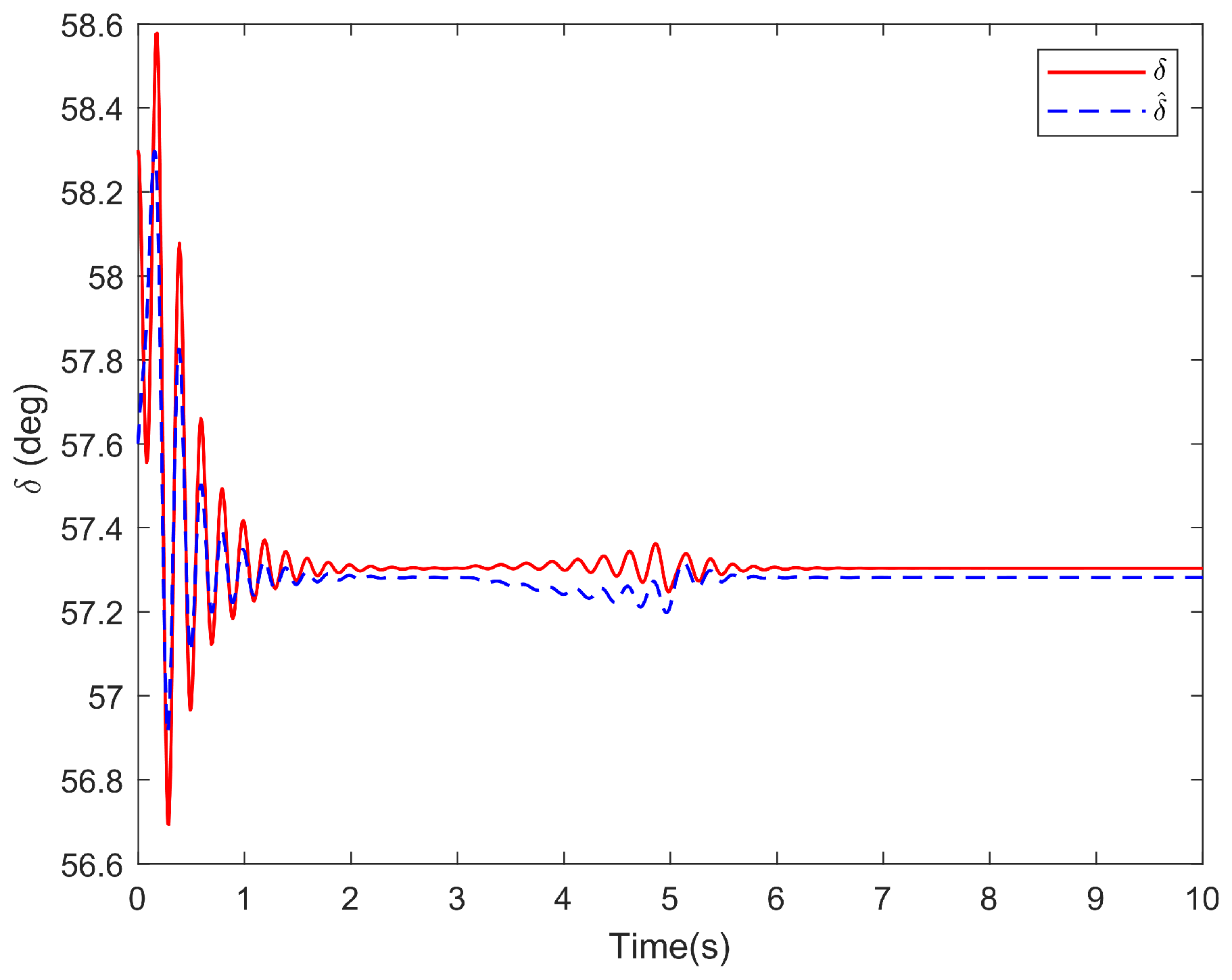
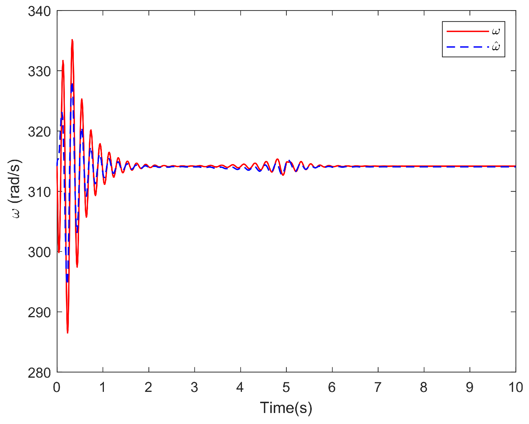
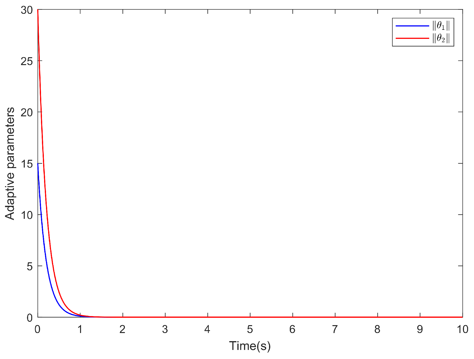
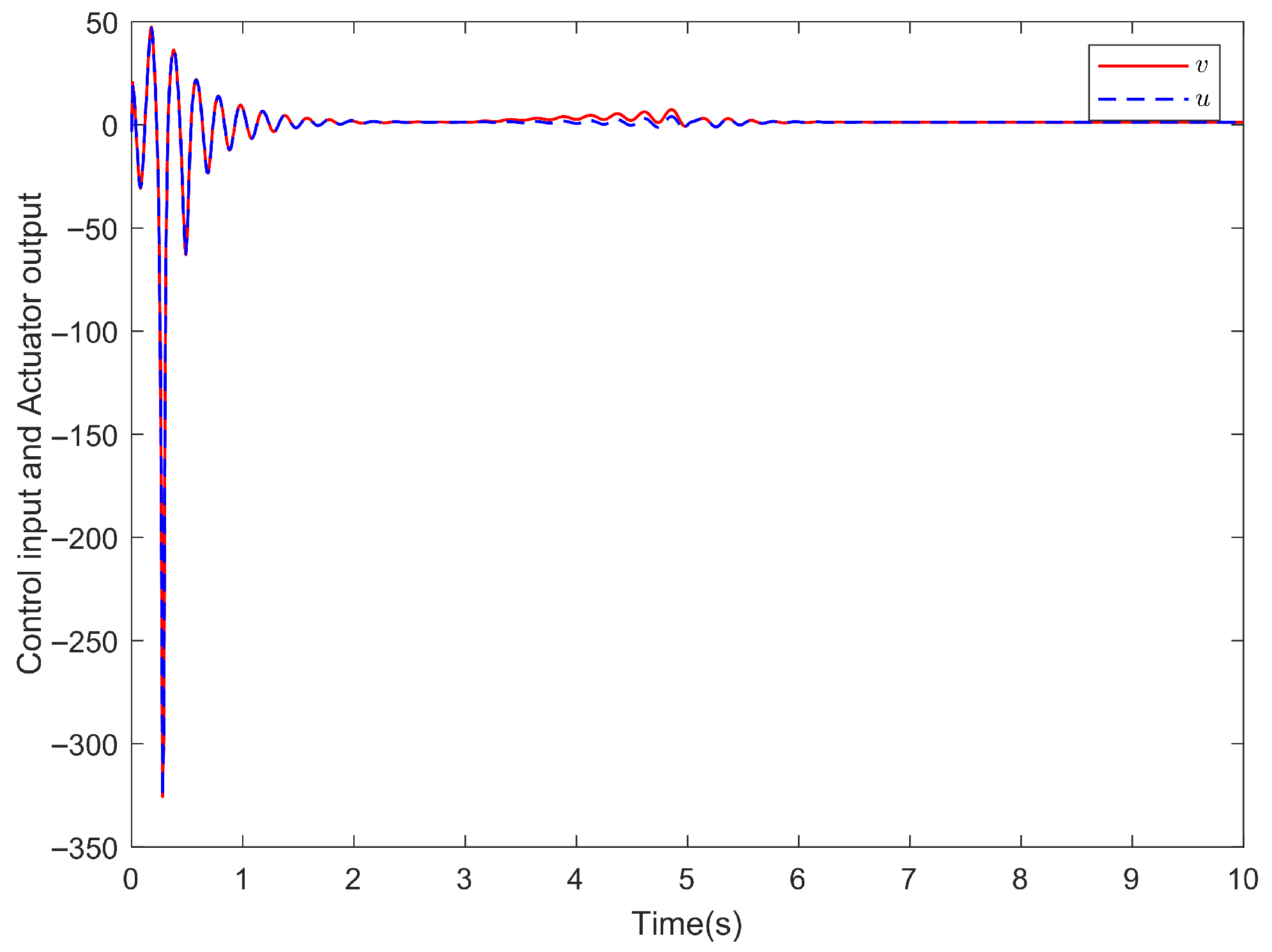
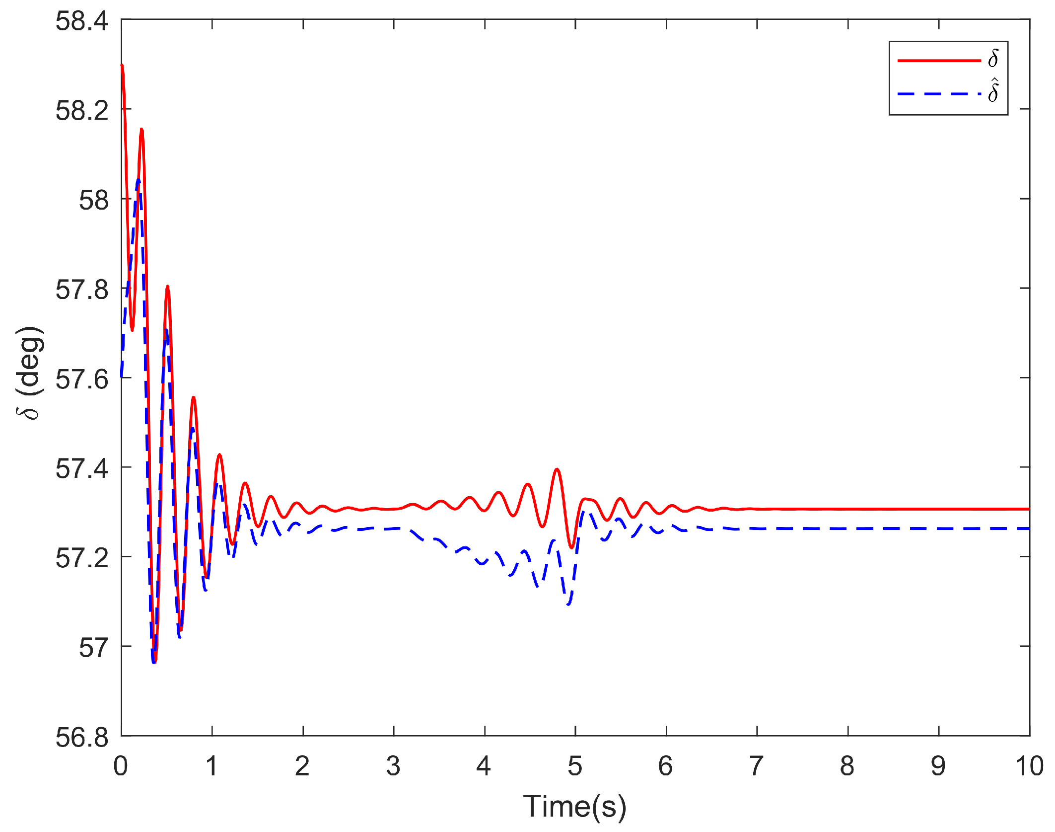
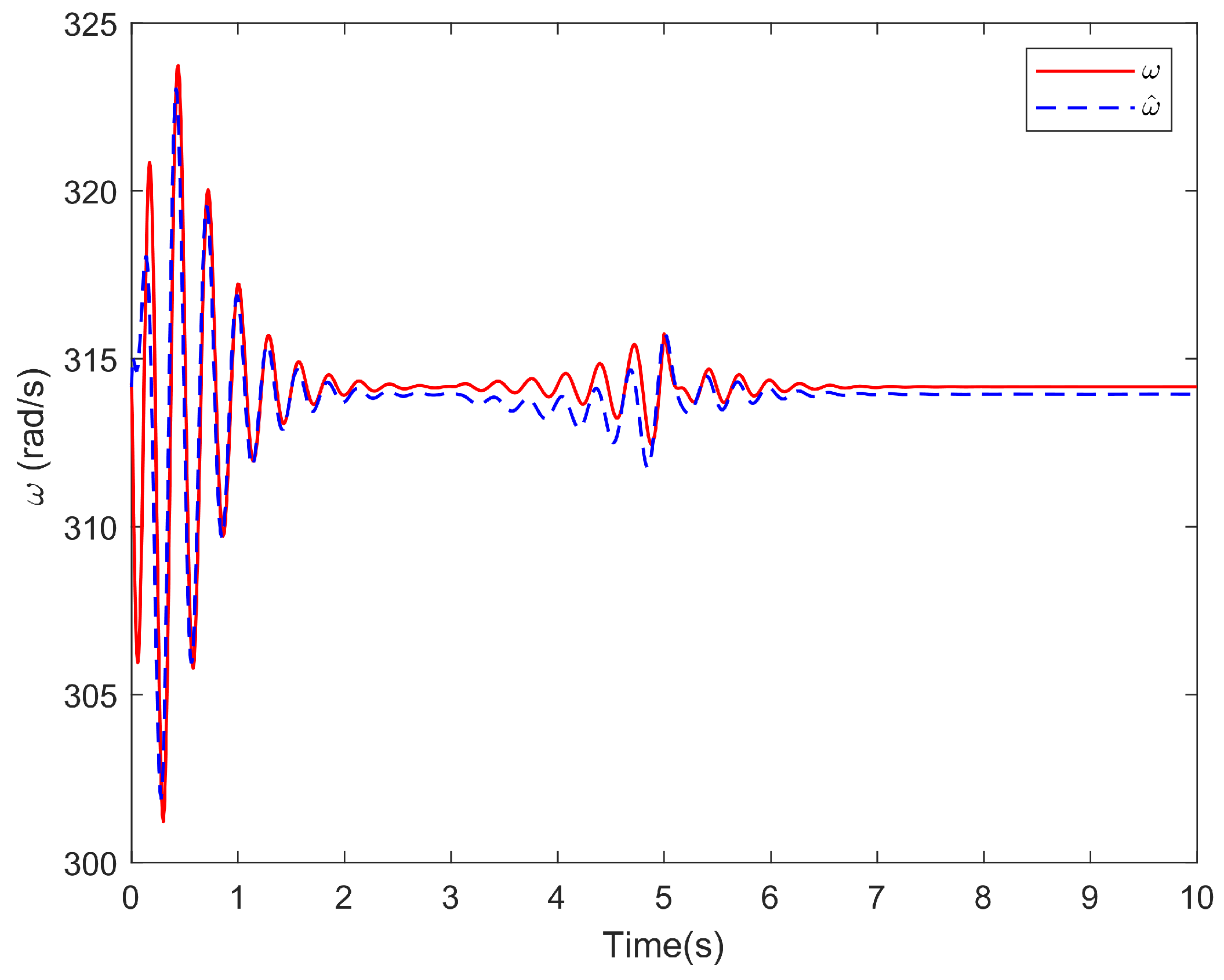
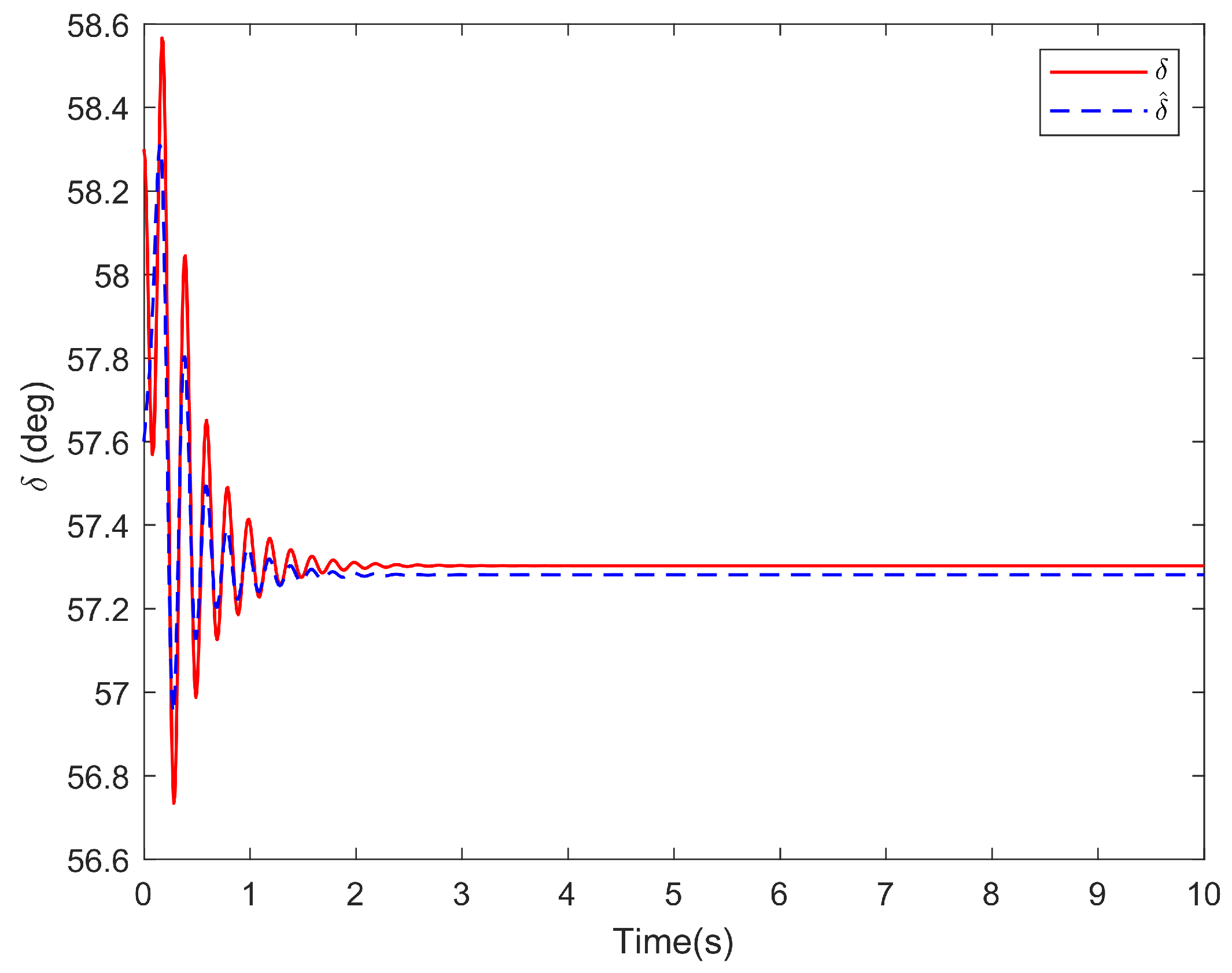
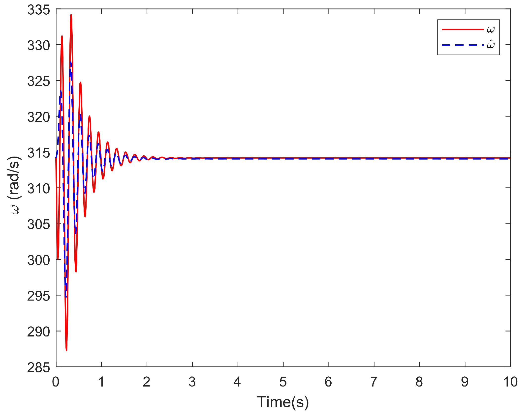
The simulation results are illustrated in Figure 2, Figure 3, Figure 4, Figure 5, Figure 6, Figure 7, Figure 8, Figure 9, Figure 10 and Figure 11. Figure 2 shows the transient response curves of the power angle $\delta$ and its estimated value $\widehat{\delta }$. Figure 3 shows the transient response curves of the rotational speed $\omega$ and its estimated value $\widehat{\omega }$. Figure 4 and Figure 5 are the waveforms of adaptive parameters $\parallel {\theta }_1\parallel$ and $\parallel {\theta }_2\parallel$ and the trajectories of the control input. As can be seen from Figure 5, actuator fault occurs when $3<t\le 5$ s, at which point the control input will change to ensure the stability of the entire control system.

Figure 2. Trajectories of $\delta$ and $\widehat{\delta }$.

Figure 3. Trajectories of $\omega$ and $\widehat{\omega }$.

Figure 4. Adaptive parameters $\parallel {\theta }_1\parallel$ and $\parallel {\theta }_2\parallel$.

Figure 5. Trajectories of control input.

Remark 7.

The selection of parameter values in this paper is based on extensive practical experience. If the simulation results are not satisfactory, appropriately increasing the values of k and l can enhance the robustness of the controller to the overall system. However, excessively large values will require a larger control input u. The filter parameter ${\omega }_p$ determines the overall waveform quality; if it is set too small, high-frequency noise cannot be effectively filtered out.

4.2. Comparative Analysis of Adaptability

To further illustrate the effectiveness and superiority of the control strategy proposed in this paper, a comparative analysis will be conducted with the adaptive controller designed based on dynamic surface control technology in [13]. The simulation results are shown in Figure 6, Figure 7, Figure 8 and Figure 9.

Figure 6. Trajectories of $\delta$ and $\widehat{\delta }$ in [13].

Figure 6. Trajectories of $\delta$ and $\widehat{\delta }$ in [13].

Figure 7. Trajectories of $\omega$ and $\widehat{\omega }$ in [13].

Figure 7. Trajectories of $\omega$ and $\widehat{\omega }$ in [13].

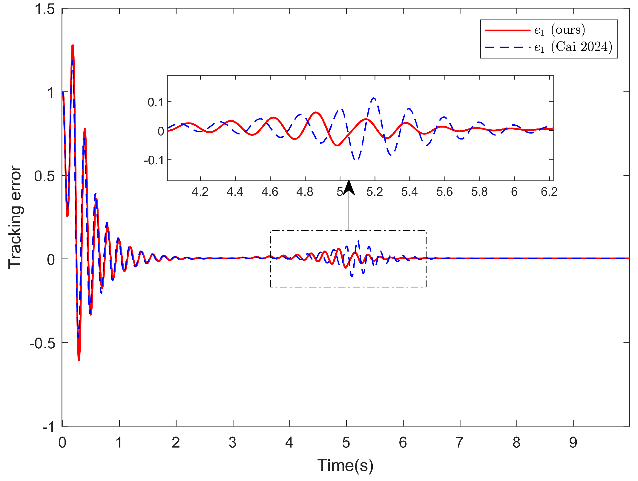
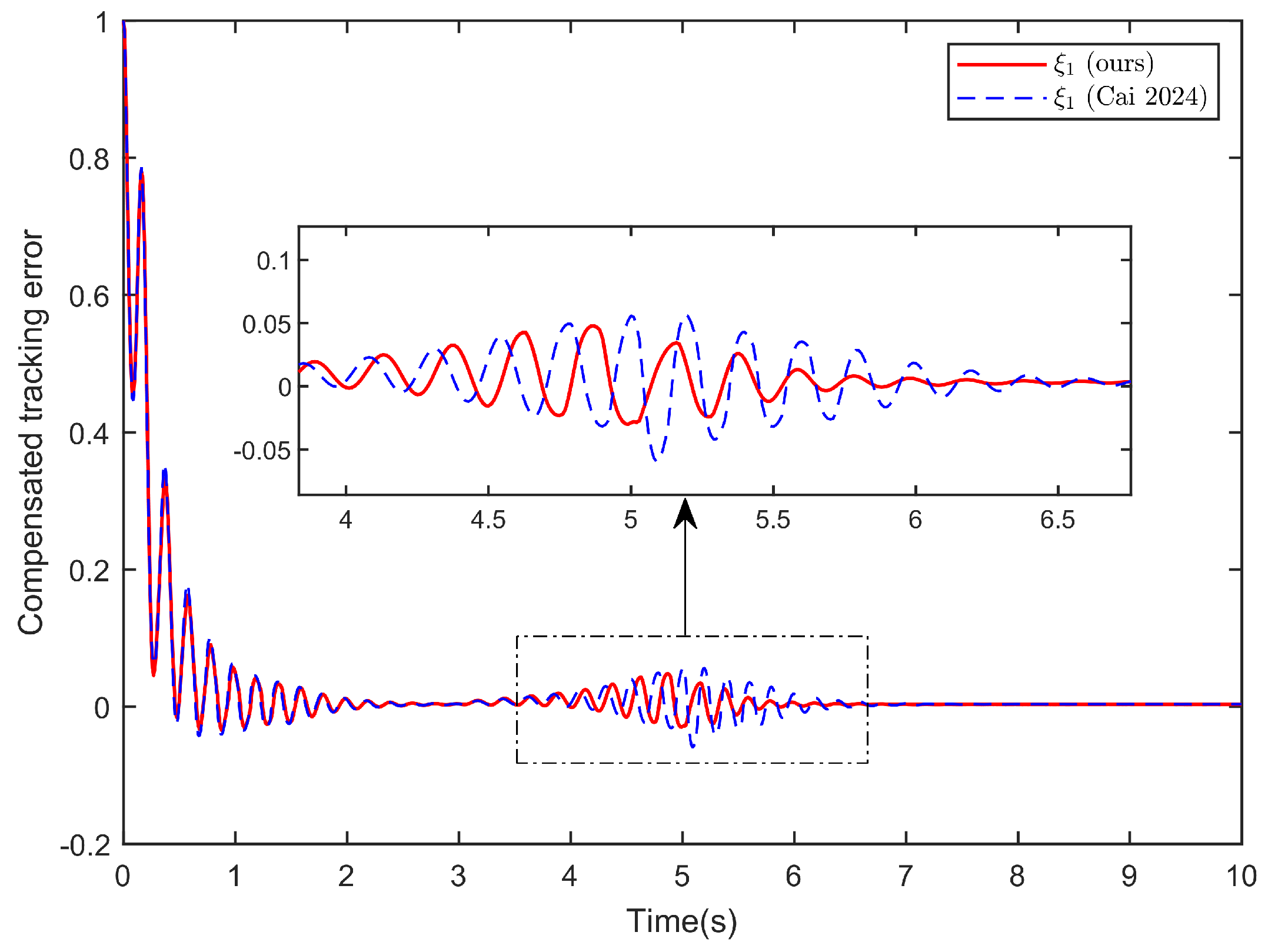
It can be seen from Figure 6 and Figure 7 that the control strategy used in [13] shows a lower performance in estimating $\delta$ and $\omega$ compared to the results shown in Figure 2 and Figure 3 of this paper. Figure 8 and Figure 9 show the tracking error and the compensated tracking error, respectively. It can be clearly observed that both the tracking error and the compensated tracking error in this paper are smaller than those in [13] and converge more rapidly to a small vicinity around zero, and the compensated tracking error exhibits lower overshoot. This demonstrates the effectiveness of the compensation signal design proposed in this paper for the TCSC single-machine infinite-bus system. The boundedness of all signals in the closed-loop system is guaranteed, as evidenced by the simulation results, which clearly illustrate the effective tracking performance of the proposed approach.

Figure 8. Trajectory for $e_1$ [13].

Figure 8. Trajectory for $e_1$ [13].

Figure 9. Compensated tracking error ${\xi }_1$ [13].

Figure 9. Compensated tracking error ${\xi }_1$ [13].

4.3. Fault-FreeComparative Analysis

Next, we present a set of figures showing the transient response curves of the power angle $\delta$ and the transient response curves of the rotational speed under fault-free conditions for comparative analysis with Figure 2 and Figure 3.

It can be observed from Figure 10 and Figure 11 that the controller designed in this paper demonstrates excellent control performance both under fault-free and fault conditions. Even in the presence of faults, the estimates of power angle and rotational speed closely match the actual values, which indicates the effectiveness of the proposed controller and the fuzzy state observer in addressing such problems.

Remark 8.

In previous traditional studies on nonlinear power systems, such as in [12], the work has remained at the level of state feedback and assumes fault-free system conditions. However, with the evolution of practical application scenarios, it is often necessary to simulate and analyze faults occurring in actual models. This paper places greater emphasis on this aspect and investigates new fault-tolerant control strategies to address the problem of unmeasurable states.

Remark 9.

While the control strategy proposed in this paper demonstrates excellent performance, it also has certain limitations. Specifically, the control method is only applicable to nonlinear systems that can be generalized into system (A1) and it relies on accurate models and parameters. If the parameters change, the method’s sensitivity to such variations may lead to degraded control performance. In future work, we will consider further optimizing the control model by incorporating excitation control and adapting and implementing the designed controller into practical FACTS devices.

Figure 10. Trajectories of $\delta$ and $\widehat{\delta }$ under fault-free conditions.

Figure 10. Trajectories of $\delta$ and $\widehat{\delta }$ under fault-free conditions.

Figure 11. Trajectories of $\omega$ and $\widehat{\omega }$ under fault-free conditions.

Figure 11. Trajectories of $\omega$ and $\widehat{\omega }$ under fault-free conditions.

Remark 10.

Existing studies on adaptive fuzzy control for SMIB/TCSC systems predominantly rely on state feedback (Table 1), which is inadequate for complex power systems [35,36]. This paper employs output feedback to address scenarios with unmeasurable states, reducing sensor dependence, simplifying wiring, cutting costs, and improving robustness. While command-filtered backstepping mitigates complexity explosion in nonlinear systems, conventional dynamic surface control introduces phase lag without compensation, harming performance [13]. Our command-filtering approach avoids these drawbacks in faulty nonlinear power systems, achieving better tracking. For actuator faults, instead of typical adaptive/projection-based compensation [24,25,26], we innovatively compensate via coordinate transformation in output feedback, attaining superior control.

Table 1. Comparison of the proposed methodology and model with other studies.

Different Aspects for Comparison	References	Feedback Control Strategy	Actuator Faults	Command Filter
Adaptive fuzzy control for SMIB/TCSC systems	[35]	State feedback	–	–
	[36]	State feedback	–	–
Command-filtered backstepping-based methods	[12]	State feedback	–	✓
	[13]	State feedback	–	✓
	[39]	State feedback	–	✓
Fault-tolerant control in nonlinear systems	[24]	Output feedback	✓	–
	[25]	State feedback	✓	–
This work		Output feedback	✓	✓

✓: considered; –: no consideration.

5. Conclusions

This paper has proposed a command-filtered fuzzy adaptive control strategy for nonlinear TCSC systems with actuator faults, unknown nonlinearities, and unmeasurable states. To broaden the method’s applicability, the SMIB system with TCSC has been transformed into a nonlinear representation that retains the power system’s intrinsic nonlinear dynamics. A state observer has been designed to estimate the unavailable system states. Based on the observer outputs, a fuzzy control algorithm has been employed to approximate the uncertain nonlinearities. Furthermore, an adaptive output feedback controller incorporating command filtering has been developed, ensuring system stability while preventing the explosion of complexity. The effectiveness of the proposed method has been validated through simulations conducted on the TCSC-based SMIB system.

Appendix A.1. Description of N-Dimensional Systems

To enhance the applicability of the proposed control scheme, we extend its scope from a second-order nonlinear power system (2) to encompass a broader range of n-dimensional nonlinear systems. That is to say, all nonlinear systems that conform to the following n-dimensional system can be controlled and solved using the controller designed in this paper. Then, system (3) can be rewritten as follows:

$$\left\{\begin{array}{c}{\dot{x}}_i=f_i\left({\overline{x}}_i\right)+x_{i+1}+d_i\left(t\right),i=1,\dots ,n-1\hfill \\ {\dot{x}}_n=f_n\left({\overline{x}}_n\right)+g_n\left({\overline{x}}_n\right)u^f+d_n\left(t\right)\hfill \\ y=x_1\hfill \end{array}\right.$$

(A1)

Among them, ${\overline{x}}_i={[x_1,x_2,\dots ,x_i]}^T\in R^i$, ${\overline{x}}_n={[x_1,x_2,\dots ,x_n]}^T\in R^n$, and $u^f\in R$ represent the system state vector and control input, respectively; $f_i\left({\overline{x}}_i\right)$ is an unknown smooth nonlinear function; $g\left(\overline{x}\right)$ denotes a known smooth bounded continuous function, satisfying $g(·)\ne 0$ and $\left|g(·)\right|\le \overline{g}$; and $d_i\left(t\right)$ is an unknown external system disturbance, satisfying $\overline{d_i}>0$ and $\left|d_i\left(t\right)\right|\le {\overline{d}}_i$, and only the output $y=x_1$ is measurable.

Appendix A.2. Controller Design

We define the tracking error:

$$\left\{\begin{array}{c}{z}_1=X_1\hfill \\ z_i={\widehat{X}}_i-x_{i,c},i=2,\dots ,n\hfill \end{array}\right.$$

(A2)

where $x_{i,c}$ is the output of the command filter. The designed command filter form is as follows

$$\left\{\begin{array}{c}{\dot{\phi }}_{i,1}={\omega }_p{\phi }_{i,2},i=1,\dots ,n-1\hfill \\ {\dot{\phi }}_{i,2}=-2m_1{\omega }_p{\phi }_{i,2}-{\omega }_p\left({\phi }_{i,1}-{\alpha }_i\right)\hfill \end{array}\right.$$

(A3)

where ${\phi }_{i,1}\left(0\right)={\alpha }_i\left(0\right)$, and ${\alpha }_i$ is the control input.

We design a compensation signal to eliminate the error caused by the command filter:

$$\left\{\begin{array}{c}{\dot{r}}_1=-k_1{r}_1+r_2+\left(x_{2,c}-{\alpha }_1\right)-l_1\mathrm{sign}\left(r_1\right),i=1,\dots ,n-1\hfill \\ {\dot{r}}_i=-k_i{r}_i-r_{i-1}+r_{i+1}+\left(x_{i+1,c}-{\alpha }_i\right)-l_i\mathrm{sign}\left(r_i\right)\hfill \\ {\dot{r}}_n=-k_n{r}_n-r_{n-1}-l_n\mathrm{sign}\left(r_n\right)\hfill \end{array}\right.$$

(A4)

where $r_i\left(0\right)=0$, $k_i>0$ and $l_i>0$ are designed constants. Then the compensated tracking errors are defined as follows

$${\xi }_i=z_i-r_i(i=1,2,\dots ,n)$$

(A5)

The first step remains identical to the previous one. Below, we will proceed directly to the design of step i.

Step i: 

The derivative of ${\xi }_i$ is $\left(i=2,\dots ,n-1\right)$:

$$\begin{array}{cc}\hfill {\dot{\xi }}_i& ={\dot{z}}_i-{\dot{r}}_i\hfill \\ \hfill & ={\dot{\widehat{X}}}_i-{\dot{x}}_{i,c}-{\dot{r}}_i\hfill \\ \hfill & ={\xi }_{i+1}+l_i{e}_1+{\alpha }_i+k_i{r}_i+r_{i-1}-{\dot{x}}_{i,c}+l_i\mathrm{sign}\left(r_i\right)\hfill \\ \hfill & +{\widehat{\theta }}_i^T{S}_i\left({\widehat{\overline{X}}}_i\right)+{\tilde{\theta }}_i^T{S}_i\left({\widehat{\overline{X}}}_i\right)-{\tilde{\theta }}_i^T{S}_i\left({\widehat{\overline{X}}}_i\right)\hfill \end{array}$$

(A6)

Then, we select the following Lyapunov function:

$$V_i=V_{i-1}+{\displaystyle \frac{1}{2}}{\xi }_i^2+{\displaystyle \frac{1}{2{\mu }_i}}{\tilde{\theta }}_i^T{\tilde{\theta }}_i$$

(A7)

Differentiating Equation (A7), we obtain that

$$\begin{array}{cc}\hfill {\dot{V}}_i& ={\dot{V}}_{i-1}+{\xi }_i{\dot{\xi }}_i-{\displaystyle \frac{1}{{\mu }_i}}{\tilde{\theta }}_i^T{\dot{\widehat{\theta }}}_i\hfill \\ \hfill & \le -G_{i-1}{\parallel e\parallel }^2+\sum _{j=1}^n{\tilde{\theta }}_j^T{\tilde{\theta }}_j+J_{i-1}+\sum _{j=1}^{i-1}{\displaystyle \frac{{\sigma }_j{\tilde{\theta }}_j^T{\widehat{\theta }}_j}{{\mu }_j}}-\sum _{j=1}^{i-1}{k}_j{\xi }_j^2+{\xi }_{i-1}{\xi }_i\hfill \\ \hfill & +\sum _{j=1}^{i-1}{\displaystyle \frac{1}{2}}{\tilde{\theta }}_j^T{\tilde{\theta }}_j-{\displaystyle \frac{1}{{\mu }_i}}{\tilde{\theta }}_i^T{\dot{\widehat{\theta }}}_i+{\xi }_i({\xi }_{i+1}+l_i{e}_1+{\alpha }_i+k_i{r}_i+r_{i-1}-{\dot{x}}_{i,c}\hfill \\ \hfill & +{\widehat{\theta }}_i^T{S}_i\left({\widehat{\overline{X}}}_i\right)+{\tilde{\theta }}_i^T{S}_i\left({\widehat{\overline{X}}}_i\right)-{\tilde{\theta }}_i^T{S}_i\left({\widehat{\overline{X}}}_i\right)+l_i\mathrm{sign}\left(r_i\right))\hfill \end{array}$$

(A8)

By using Young’s inequality, we can get

$${\xi }_i{l}_i{e}_1\le {\displaystyle \frac{l_i}{2}}{\xi }_i^2+{\displaystyle \frac{l_i}{2}}{\parallel e\parallel }^2$$

(A9)

$${\xi }_i\left(l_i{e}_1-{\tilde{\theta }}_i^T{S}_i\left({\widehat{\overline{X}}}_i\right)\right)\le \left({\displaystyle \frac{1}{2}}+{\displaystyle \frac{l_i}{2}}\right){\xi }_i^2+{\displaystyle \frac{1}{2}}\left({\parallel e\parallel }^2+{\tilde{\theta }}_i^T{\tilde{\theta }}_i\right)$$

(A10)

$${\xi }_i{l}_i\mathrm{sign}\left(r_i\right)\le {\displaystyle \frac{{\xi }_i^2}{2}}+{\displaystyle \frac{{\overline{l}}_i^2}{2}}$$

(A11)

and then, substituting (A9)∼(A11) into (A8), we can get

$$\begin{array}{cc}\hfill {\dot{V}}_i& \le -G_i{\parallel e\parallel }^2+\sum _{j=1}^n{\tilde{\theta }}_j^T{\tilde{\theta }}_j+J_i+\sum _{j=1}^{i-1}{\displaystyle \frac{{\sigma }_j{\tilde{\theta }}_j^T{\widehat{\theta }}_j}{{\mu }_j}}-\sum _{j=1}^{i-1}{k}_j{\xi }_j^2+{\xi }_{i-1}{\xi }_i+\sum _{j=2}^i{\displaystyle \frac{1}{2}}{\tilde{\theta }}_j^T{\tilde{\theta }}_j\hfill \\ \hfill & +{\xi }_i\left(\left(1+{\displaystyle \frac{l_i}{2}}\right){\xi }_i+{\xi }_{i+1}+{\alpha }_i+k_i{r}_i+r_{i-1}-{\dot{x}}_{i,c}+{\widehat{\theta }}_i^T{S}_i\left({\widehat{\overline{X}}}_i\right)\right)\hfill \\ \hfill & +{\displaystyle \frac{1}{{\mu }_i}}{\tilde{\theta }}_i^T\left({\mu }_i{\xi }_i{S}_i\left({\widehat{\overline{X}}}_i\right)-{\dot{\widehat{\theta }}}_i\right)\hfill \end{array}$$

(A12)

where $G_i=G_{i-1}-{\displaystyle \frac{1}{2}}$ and $J_i=J_{i-1}+{\displaystyle \frac{{\overline{l}}_i^2}{2}}$.

The virtual control law ${\alpha }_i$ and the adaptive law ${\dot{\widehat{\theta }}}_i$ are designed with the following expressions:

$${\alpha }_i=-k_i{z}_i-z_{i-1}-\left(1+{\displaystyle \frac{l_i}{2}}\right){\xi }_i-{\widehat{\theta }}_i^T{S}_i\left({\widehat{\overline{X}}}_i\right)+{\dot{x}}_{i,c}$$

(A13)

$${\dot{\widehat{\theta }}}_i={\mu }_i{\xi }_i{S}_i\left({\widehat{\overline{X}}}_i\right)-{\sigma }_i{\widehat{\theta }}_i$$

(A14)

Combined with (A13) and (A14), (A12) can be rewritten as

$${\dot{V}}_i\le -G_i{\parallel e\parallel }^2+\sum _{j=1}^n{\tilde{\theta }}_j^T{\tilde{\theta }}_j+J_i+\sum _{j=1}^i{\displaystyle \frac{{\sigma }_j{\tilde{\theta }}_j^T{\widehat{\theta }}_j}{{\mu }_j}}-\sum _{j=1}^i{k}_j{\xi }_j^2+{\xi }_i{\xi }_{i+1}+\sum _{j=2}^i{\displaystyle \frac{1}{2}}{\tilde{\theta }}_j^T{\tilde{\theta }}_j$$

(A15)

Step n: 

The derivative of ${\xi }_n$ is

$$\begin{array}{cc}\hfill {\dot{\xi }}_n& ={\dot{z}}_n-{\dot{r}}_n\hfill \\ \hfill & ={\dot{\widehat{X}}}_n-{\dot{x}}_{n,c}-{\dot{r}}_n\hfill \\ \hfill & =G_n\left({\overline{X}}_n\right)v\left(t\right)+{\widehat{\theta }}_n^T{S}_n\left({\widehat{\overline{X}}}_n\right)+l_n\left(Y-{\widehat{X}}_1\right)+{\tilde{\theta }}_n^T{S}_n\left({\widehat{\overline{X}}}_n\right)\hfill \\ \hfill & -{\tilde{\theta }}_n^T{S}_n\left({\widehat{\overline{X}}}_n\right)-{\dot{x}}_{n,c}+k_n{r}_n+r_{n-1}+l_n\mathrm{sign}\left(r_n\right)\hfill \end{array}$$

(A16)

We choose the following Lyapunov function:

$$V_n=V_{n-1}+{\displaystyle \frac{1}{2}}{\xi }_n^2+{\displaystyle \frac{1}{2{\mu }_n}}{\tilde{\theta }}_n^T{\tilde{\theta }}_n$$

(A17)

Then we can get ${\dot{V}}_n$ as follows

$$\begin{array}{cc}\hfill {\dot{V}}_n& ={\dot{V}}_{n-1}+{\xi }_n{\dot{\xi }}_n-{\displaystyle \frac{1}{{\mu }_n}}{\tilde{\theta }}_n^T{\dot{\widehat{\theta }}}_n\hfill \\ \hfill & \le -G_{n-1}{\parallel e\parallel }^2+\sum _{j=1}^n{\tilde{\theta }}_j^T{\tilde{\theta }}_j+J_{n-1}+\sum _{j=1}^{n-1}{\displaystyle \frac{{\sigma }_j{\tilde{\theta }}_j^T{\widehat{\theta }}_j}{{\mu }_j}}-\sum _{j=1}^{n-1}{k}_j{\xi }_j^2+{\xi }_{n-1}{\xi }_n+\sum _{j=2}^{n-1}{\displaystyle \frac{1}{2}}{\tilde{\theta }}_j^T{\tilde{\theta }}_j\hfill \\ \hfill & +{\xi }_n(G_n\left({\overline{X}}_n\right)v\left(t\right)+{\widehat{\theta }}_n^T{S}_n\left({\widehat{\overline{X}}}_n\right)+l_n\left(Y-{\widehat{X}}_1\right)+{\tilde{\theta }}_n^T{S}_n\left({\widehat{\overline{X}}}_n\right)-{\tilde{\theta }}_n^T{S}_n\left({\widehat{\overline{X}}}_n\right)\hfill \\ \hfill & -{\dot{x}}_{n,c}+k_n{r}_n+r_{n-1}+l_n\mathrm{sign}\left(r_n\right))-{\displaystyle \frac{1}{{\mu }_n}}{\tilde{\theta }}_n^T{\dot{\widehat{\theta }}}_n\hfill \end{array}$$

(A18)

By using Young’s inequality, we can get

$${\xi }_n{l}_n{e}_1\le {\displaystyle \frac{l_n}{2}}{\xi }_n^2+{\displaystyle \frac{l_n}{2}}{\parallel e\parallel }^2$$

(A19)

Thus, by Young’s inequality, we can get:

$${\xi }_n\left(l_n{e}_1-{\tilde{\theta }}_n^T{S}_n\left({\widehat{\overline{X}}}_n\right)\right)\le \left({\displaystyle \frac{1}{2}}+{\displaystyle \frac{l_n}{2}}\right){\xi }_n^2+{\displaystyle \frac{1}{2}}\left({\parallel e\parallel }^2+{\tilde{\theta }}_n^T{\tilde{\theta }}_n\right)$$

(A20)

$${\xi }_n{l}_n\mathrm{sign}\left(r_n\right)\le {\displaystyle \frac{{\xi }_n^2}{2}}+{\displaystyle \frac{{\overline{l}}_n^2}{2}}$$

(A21)

and then, substituting (A19)∼(A21) into (A18), we can get

$$\begin{array}{cc}\hfill {\dot{V}}_n& \le -G_n{\parallel e\parallel }^2+\sum _{j=1}^n{\tilde{\theta }}_j^T{\tilde{\theta }}_j+J_n+\sum _{j=1}^{n-1}{\displaystyle \frac{{\sigma }_j{\tilde{\theta }}_j^T{\widehat{\theta }}_j}{{\mu }_j}}-\sum _{j=1}^{n-1}{k}_j{\xi }_j^2+{\xi }_{n-1}{\xi }_n+\sum _{j=2}^n{\displaystyle \frac{1}{2}}{\tilde{\theta }}_j^T{\tilde{\theta }}_j\hfill \\ \hfill & +{\xi }_n\left(\left(1+{\displaystyle \frac{l_n}{2}}\right){\xi }_n+G_n\left({\overline{X}}_n\right)v\left(t\right)+{\widehat{\theta }}_n^T{S}_n\left({\widehat{\overline{X}}}_n\right)-{\dot{x}}_{n,c}+k_n{r}_n+r_{n-1}\right)\hfill \\ \hfill & +{\displaystyle \frac{1}{{\mu }_n}}{\tilde{\theta }}_n^T\left({\mu }_n{\xi }_n{S}_n\left({\widehat{\overline{X}}}_n\right)-{\dot{\widehat{\theta }}}_n\right)\hfill \end{array}$$

(A22)

where $G_n=G_{n-1}-{\displaystyle \frac{1}{2}}$ and $J_n=J_{n-1}+{\displaystyle \frac{{\overline{l}}_n^2}{2}}$.

We design the final controller $v\left(t\right)$ and the adaptive law ${\dot{\widehat{\theta }}}_n$ as:

$$v\left(t\right)={\displaystyle \frac{1}{G_n\left({\overline{X}}_n\right)}}\left[-k_n{z}_n-z_{n-1}-\left(1+{\displaystyle \frac{l_n}{2}}\right){\xi }_n-{\widehat{\theta }}_n^T{S}_n\left({\widehat{\overline{X}}}_n\right)+{\dot{x}}_{n,c}\right]$$

(A23)

$${\dot{\widehat{\theta }}}_n={\mu }_n{\xi }_n{S}_n\left({\widehat{\overline{X}}}_n\right)-{\sigma }_n{\widehat{\theta }}_n$$

(A24)

Combined with (A23) and (A24), we can obtain that

$${\dot{V}}_n\le -G_n{\parallel e\parallel }^2+\sum _{j=1}^n{\tilde{\theta }}_j^T{\tilde{\theta }}_j+J_n+\sum _{j=1}^n{\displaystyle \frac{{\sigma }_j{\tilde{\theta }}_j^T{\widehat{\theta }}_j}{{\mu }_j}}-\sum _{j=1}^n{k}_j{\xi }_j^2+\sum _{j=2}^n{\displaystyle \frac{1}{2}}{\tilde{\theta }}_j^T{\tilde{\theta }}_j$$

(A25)

Regarding the stability of the system, the reader can verify it independently by following the procedure presented in the main text.

References

1. Siad, S.B.; Malkawi, A.; Damm, G.; Lopes, L.; Dol, L.G. Nonlinear control of a DC MicroGrid for the integration of distributed generation based on different time scales. Int. J. Electr. Power Energy Syst. 2019, 111, 93–100. [Google Scholar] [CrossRef] [Scilit]
2. Hekss, Z.; Abouloifa, A.; Lachkar, I.; El Aroudi, A.; Echalih, S.; Al-Numay, M.; Giri, F. Advanced nonlinear controller of single-phase shunt active power filter interfacing solar photovoltaic source and electrical power grid. Int. Trans. Electr. Energy Syst. 2021, 31, e13237. [Google Scholar] [CrossRef] [Scilit]
3. Del Rosso, A.D.; Canizares, C.A.; Dona, V.M. A study of TCSC controller design for power system stability improvement. IEEE Trans. Power Syst. 2003, 18, 1487–1496. [Google Scholar] [CrossRef]
4. Naresh, G.; Raju, M.R.; Narasimham, S. Coordinated design of power system stabilizers and TCSC employing improved harmony search algorithm. Swarm Evol. Comput. 2016, 27, 169–179. [Google Scholar] [CrossRef] [Scilit]
5. Xu, X.; Zhao, J.; Xu, Z.; Chai, S.; Li, J.; Yu, Y. Stochastic optimal TCSC placement in power system considering high wind power penetration. IET Gener. Transm. Distrib. 2018, 12, 3052–3060. [Google Scholar] [CrossRef] [Scilit]
6. Maddela, C.O.; Subudhi, B. Robust wide-area TCSC controller for damping enhancement of inter-area oscillations in an interconnected power system with actuator saturation. Int. J. Electr. Power Energy Syst. 2019, 105, 478–487. [Google Scholar] [CrossRef] [Scilit]
7. Liu, D.; Liu, Y.; Alsaadi, F.E. A new framework for output feedback controller design for a class of discrete-time stochastic nonlinear system with quantization and missing measurement. Int. J. Gen. Syst. 2016, 45, 517–531. [Google Scholar] [CrossRef] [Scilit]
8. Yu, J.; Shi, P.; Dong, W.; Yu, H. Observer and command-filter-based adaptive fuzzy output feedback control of uncertain nonlinear systems. IEEE Trans. Ind. Electron. 2015, 62, 5962–5970. [Google Scholar] [CrossRef] [Scilit]
9. Wang, H.; Li, Y.; Zhu, Q.; Deng, F. Finite-time output-feedback stabilization for a class of switched stochastic planar systems with asymmetric time-varying output constraints. Sci. China Inf. Sci. 2025, 68, 202202. [Google Scholar] [CrossRef] [Scilit]
10. Zhu, Q.; Wang, H. Output feedback stabilization of stochastic feedforward systems with unknown control coefficients and unknown output function. Automatica 2018, 87, 166–175. [Google Scholar] [CrossRef] [Scilit]
11. Wang, H.; Zhu, Q. Adaptive output feedback control of stochastic nonholonomic systems with nonlinear parameterization. Automatica 2018, 98, 247–255. [Google Scholar] [CrossRef] [Scilit]
12. Xu, W.; Li, Z.; Cui, G.; Wang, C.; Hu, F. Fuzzy adaptive finite time command filter backstepping control of power system. Int. J. Control. Autom. Syst. 2021, 19, 3812–3822. [Google Scholar] [CrossRef] [Scilit]
13. Cai, G.; Xiao, Y.; Wei, H.; Wu, T.; Hou, M. Robust adaptive dynamic surface control of high-order strict feedback systems based on fully actuated system approach. Int. J. Syst. Sci. 2024, 55, 2464–2477. [Google Scholar] [CrossRef] [Scilit]
14. Zhou, J.; Zhang, C.; Wen, C. Robust adaptive output control of uncertain nonlinear plants with unknown backlash nonlinearity. IEEE Trans. Autom. Control 2007, 52, 503–509. [Google Scholar] [CrossRef] [Scilit]
15. KrstiC, M.; KokotoviC, P.V. Adaptive nonlinear output-feedback schemes with Marino-Tomei controller. IEEE Trans. Autom. Control 1996, 41, 274–280. [Google Scholar] [CrossRef] [Scilit]
16. Wu, Z.; Xie, X.; Shi, P. Robust adaptive output-feedback control for nonlinear systems with output unmodeled dynamics. Int. J. Robust Nonlinear Control IFAC-Affil. J. 2008, 18, 1162–1187. [Google Scholar] [CrossRef] [Scilit]
17. Islam, S.; Liu, P.X.; El Saddik, A. Observer-based adaptive output feedback control for miniature aerial vehicle. IEEE Trans. Ind. Electron. 2017, 65, 470–477. [Google Scholar] [CrossRef] [Scilit]
18. Zhang, M.; Shi, P.; Shen, C.; Wu, Z. Static output feedback control of switched nonlinear systems with actuator faults. IEEE Trans. Fuzzy Syst. 2019, 28, 1600–1609. [Google Scholar] [CrossRef] [Scilit]
19. Shan, H.; Jiang, Y.; Liang, H.; Wang, S.; Lam, H.K. Fuzzy Adaptive Containment Control for Nonlinear Multi-Manipulator Systems With Actuator Faults and Predefined Accuracy. IEEE Trans. Netw. Sci. Eng. 2024, 11, 1510–1523. [Google Scholar] [CrossRef] [Scilit]
20. Yang, W.; Jiang, Y.; He, X.; Zhu, Y.; Wang, S. Feasibility Conditions-Free Prescribed Performance Decentralized Fault-Tolerant Neural Control of Constrained Large-Scale Systems. IEEE Trans. Syst. Man Cybern. Syst. 2023, 53, 3152–3164. [Google Scholar] [CrossRef] [Scilit]
21. Chakravarty, A.; Mahanta, C.; Wang, W.; Kar, I. A switching-free multiple-model approach for adaptive FTC of non-Lipschitz nonlinear uncertain systems under persistent actuator failures. IFAC J. Syst. Control 2022, 21, 100201. [Google Scholar] [CrossRef] [Scilit]
22. Zhang, L.; Yang, G.H. Fault-Estimation-Based Output-Feedback Adaptive FTC for Uncertain Nonlinear Systems With Actuator Faults. IEEE Trans. Ind. Electron. 2020, 67, 3065–3075. [Google Scholar] [CrossRef] [Scilit]
23. Huang, J.; Wang, H. Sensor-Enabled Nested Networked Control for Speed Synchronization and Swing Damping in Air–Ground Collaborative Distribution. Sensors 2026, 26, 92. [Google Scholar] [CrossRef] [Scilit]
24. Deng, C.; Wen, C. Distributed resilient observer-based fault-tolerant control for heterogeneous multiagent systems under actuator faults and DoS attacks. IEEE Trans. Control Netw. Syst. 2020, 7, 1308–1318. [Google Scholar] [CrossRef] [Scilit]
25. Du, C.; Li, F.; Yang, C. An improved homogeneous polynomial approach for adaptive sliding-mode control of Markov jump systems with actuator faults. IEEE Trans. Autom. Control 2019, 65, 955–969. [Google Scholar] [CrossRef] [Scilit]
26. Jin, X.; Lü, S.; Yu, J. Adaptive NN-based consensus for a class of nonlinear multiagent systems with actuator faults and faulty networks. IEEE Trans. Neural Netw. Learn. Syst. 2021, 33, 3474–3486. [Google Scholar] [CrossRef] [Scilit]
27. Ma, H.; Zhou, Q.; Ren, H.; Wang, Z. Distributed Estimator-Based Fuzzy Containment Control for Nonlinear Multi-Agent Systems With Deferred Constraints. IEEE Trans. Fuzzy Syst. 2025, 33, 2074–2083. [Google Scholar] [CrossRef] [Scilit]
28. Ji, R.; Li, D.; Ge, S.S.; Li, H. Tunnel Prescribed Control of Nonlinear Systems With Unknown Control Directions. IEEE Trans. Neural Netw. Learn. Syst. 2025, 36, 1383–1395. [Google Scholar] [CrossRef] [Scilit]
29. Hua, C.; Li, H.; Li, K.; Ding, W. Low-Computation Tracking Control of Nonlinear Systems With Asymmetric Full-State Constraints and Unknown Control Directions. IEEE Trans. Syst. Man Cybern. Syst. 2023, 53, 1051–1059. [Google Scholar] [CrossRef] [Scilit]
30. Niu, Y.; Xu, X.; Liu, M. Fixed Time Synchronization of Stochastic Takagi–Sugeno Fuzzy Recurrent Neural Networks with Distributed Delay under Feedback and Adaptive Controls. Axioms 2024, 13, 391. [Google Scholar] [CrossRef] [Scilit]
31. Jia, F.; Cao, F.; He, X. Adaptive fault-tolerant tracking control for uncertain nonlinear systems with unknown control directions and limited resolution. IEEE Trans. Syst. Man Cybern. Syst. 2022, 53, 1813–1825. [Google Scholar] [CrossRef] [Scilit]
32. Zamani, N.; Askari, J.; Kamali, M.; Kalantari, H.; Aghdam, A. Adaptive tracking control for nonlinear multi-agent systems with stuck failures and unknown control directions. J. Frankl. Inst. 2024, 361, 107059. [Google Scholar] [CrossRef] [Scilit]
33. Qian, C.; Du, H. Global output feedback stabilization of a class of nonlinear systems via linear sampled-data control. IEEE Trans. Autom. Control 2012, 57, 2934–2939. [Google Scholar] [CrossRef] [Scilit]
34. Cheng, Y.; Zhang, J.; Du, H.; Wen, G.; Lin, X. Global event-triggered output feedback stabilization of a class of nonlinear systems. IEEE Trans. Syst. Man Cybern. Syst. 2019, 51, 4040–4047. [Google Scholar] [CrossRef] [Scilit]
35. Dimirovski, G.M.; Jing, Y.W.; Li, W.L.; Liu, X.P. Adaptive back-stepping design of TCSC robust nonlinear control for power systems. Intell. Autom. Soft Comput. 2006, 12, 75–87. [Google Scholar] [CrossRef] [Scilit]
36. Sun, L.Y.; Zhao, Y. Improved adaptive backstepping sliding mode control for multi-machine system with TCSC. In Proceedings of the 2018 Chinese Control and Decision Conference (CCDC), Shenyang, China, 9–11 June 2018; IEEE: Piscataway, NJ, USA, 2018; pp. 5395–5398. [Google Scholar]
37. Li, J.; Ji, R.; Liang, X.; Yan, H.; Ge, S.S. Finite-time adaptive fuzzy control of nonlinear systems with actuator faults and input saturation. Neural Comput. Appl. 2024, 36, 3569–3581. [Google Scholar] [CrossRef] [Scilit]
38. Guo, J.; Bo, Y.; Park, J.H.; Ma, J. Adaptive neural control for nonlinear systems with actuator faults and unknown control directions via command filter. Int. J. Robust Nonlinear Control 2022, 32, 2100–2118. [Google Scholar] [CrossRef] [Scilit]
39. Xia, J.; Zhang, J.; Feng, J.; Wang, Z.; Zhuang, G. Command Filter-Based Adaptive Fuzzy Control for Nonlinear Systems With Unknown Control Directions. IEEE Trans. Syst. Man Cybern. Syst. 2021, 51, 1945–1953. [Google Scholar] [CrossRef] [Scilit]
40. Shoja-Majidabad, S.; Zirkohi, M.M. Adaptive neural dynamic surface control of load/grid connected voltage source inverters with LC/LCL filters. IFAC J. Syst. Control 2023, 26, 100230. [Google Scholar] [CrossRef] [Scilit]
Figure 2. Trajectories of δ and δ ^ .
Axioms 15 00212 g002
Figure 3. Trajectories of ω and ω ^ .
Axioms 15 00212 g003
Figure 4. Adaptive parameters θ 1 and θ 2 .
Axioms 15 00212 g004