Article

The Optimal Robust Investment Problem in the Foreign Stock Market of an Ambiguity-Averse Insurer

1
School of Mathematics and Statistics, Donghua University, Shanghai 201620, China
2
School of Economics and Management, Hebei University of Technology, Tianjin 300401, China
*
Author to whom correspondence should be addressed.
Axioms 2026, 15(1), 30; https://doi.org/10.3390/axioms15010030
Submission received: 8 November 2025 / Revised: 24 December 2025 / Accepted: 26 December 2025 / Published: 29 December 2025
(This article belongs to the Special Issue Advances in Financial Mathematics and Stochastic Processes)

Abstract

To address the need for robust investment strategies in an increasingly uncertain global market, this study focuses on an ambiguity-averse insurer facing exchange rate uncertainty while investing in a foreign stock market. The insurer’s surplus is modeled via a classical compound Poisson process, and exchange rate dynamics are captured using an Ornstein–Uhlenbeck process for the drift component. Within the framework of maximizing expected exponential utility of terminal wealth, we derive and solve the Hamilton–Jacobi–Bellman equation to characterize the optimal investment strategy and the associated value function. Finally, a numerical example illustrates how varying model parameters influences the insurer’s optimal investment behavior.

1. Introduction

The investment behavior of insurance companies plays a pivotal role in ensuring their long-term solvency and profitability. A substantial body of research has explored this topic from multiple perspectives, including investment strategy design, risk control mechanisms, and the influence of regulatory environments. The seminal study by [1] introduces continuous-time portfolio optimization models that reflect the dynamic characteristics of financial markets. Although Merton’s analysis was not originally tailored to the insurance sector, it provided a fundamental framework for maximizing the expected utility of terminal wealth, which later became instrumental in insurance-related research. Building on this foundation, the paper [2] adapted the optimization problem to an insurance context by modeling the surplus as a controlled stochastic process and aiming to maximize the insurer’s probability of survival. Together, these contributions established a classical paradigm for dynamic asset management in insurance, integrating investment returns with the inherent uncertainty of the insurer’s surplus evolution.
Investing in foreign stock markets provides numerous advantages, including diversification, access to global growth opportunities, currency diversification, and potential for higher returns. By expanding their investment horizons beyond their home country, investors can reduce risk, capitalize on global trends, and enhance their overall portfolio performance. In this paper, we assume that the insurance company is allowed to invest in the foreign stock market. Thus, the insurer should pay attention to the exchange rate. Changes in exchange rates can alter the value of assets denominated in foreign currencies. If an investor holds stocks priced in U.S. dollars and their home currency depreciates, the value of these stocks in the home currency will increase. Conversely, if the home currency appreciates, the value of foreign assets will decrease. The paper [3] studied insurers’ cross-border investment and reinsurance optimization problems while incorporating exchange rate risks within an extended CIR interest rate framework.The study [4] investigated the optimal investment problem of insurers allocating assets to foreign markets while accounting for foreign exchange rate models. In this study, we followed the convention where the exchange rate is expressed in terms of domestic currency units per unit of foreign currency. Based on [4,5], for mathematical convenience, we adopted a relatively simple stochastic model to simulate the fluctuation of the exchange rate in which the drift term followed an Ornstein–Uhlenbeck (O-U) process and the volatility rate was a constant. The presence of the O-U process was to show the effects of some government policy or market sentiment. In practice, the parameters of the O-U drift, particularly the mean reversion speed are difficult to estimate precisely. For an insurer with long-term foreign investments, misjudging these parameters can lead to significant currency-timing risks: if the insurer overestimates how quickly an exchange rate deviation will correct, it may hedge too early and forfeit profitable positions; if it underestimates the reversion speed, it may retain unhedged exposures for too long, exposing the surplus to sustained currency losses. This parameter uncertainty creates a natural source of model ambiguity that is especially pertinent for insurers, whose liability-matching and solvency requirements demand the management of long-horizon currency risk. As such, model ambiguity is considered in our model.
Real-world models often have inaccuracies or uncertainties due to simplifications, approximations, or lack of complete information. There are parameters in the model that may not be precisely known, leading to a range of possible scenarios. In our paper, we assume that the insurer has aversion to ambiguity about the inaccuracy of the model parameters—in other words, the insurance company aims to find the robust optimal investment policy in the worst-case scenario. The dominant theoretical framework for formalizing this aversion to model misspecification is the multiplier preference approach of [6]. This approach penalizes alternative models according to their relative entropy distance from a reference model, leading to a tractable robust stochastic control problem. Building upon this fundamental theoretical basis, the study [7] addressed the time inconsistency defect existing in the initial multiplier preference structure, and explicit robust portfolio strategies under the constant relative risk aversion utility setting were derived—findings that have since served as a pivotal reference for empirical research on robust investment. The paper [8] examined the optimal intertemporal asset allocation for an investor concerned with model misspecification, who employed robust decision rules to account for a mean-reverting risk premium. This article [9] explored the optimal investment strategy for an ambiguity-averse investor in a setting with stochastic interest rates. Within insurance economics, a robust framework has been systematically applied to refine core strategies. For instance, the central problem of joint reinsurance and investment has been extensively examined under criteria like mean-variance and benchmarking [10]. Subsequent studies have expanded the framework to include important practical factors, including the default risk in asset markets [11], dynamic learning about model parameters [12], and incentive conflicts in a principal-agent setting [13]. Alongside these integrated models, the framework has also been used to analyze stand-alone payout decisions, showing how ambiguity aversion leads to more conservative optimal dividend policies [14]. Furthermore, to ensure implementable multi-period plans, research employing smooth ambiguity preferences has derived time-consistent strategies [15]. The intersection of robust investment and exchange rate risk is central to our cross-border investment context. The study [16] developed a non-Gaussian dynamic currency hedging strategy for ambiguity-averse investors, showing its empirical superiority over traditional benchmarks. Building on these advances—particularly the insurer foreign-investment framework [4]—this paper further investigates the robust optimal investment problem for ambiguity-averse insurers. To formalize these distorted scenarios, a measure transformation was employed, and the corresponding Radon–Nikodym (R–N) derivative describes how the alternative measure deviates from the baseline measure. The R–N density provides a convenient way to express changes in the drift or other model components that arise under uncertainty. By integrating this likelihood ratio into the optimization framework—typically through a penalty term that captures the degree of ambiguity aversion—the problem can be recast as an interaction between the decision maker and an adversarial force representing model uncertainty. This formulation offers a clear and analytically manageable structure for examining how ambiguity influences optimal investment behavior.
We aim to maximize the expected utility of terminal wealth. Different optimization objectives have been studied by scholars. The paper [17] studied the optimal investment and reinsurance problem, aiming to minimize the probability of ultimate ruin. The study [18] investigated the optimal proportional reinsurance under group correlation with the mean-variance criterion. There are also a number of scholars exploring the optimization problem of maximizing the terminal utility, such as, for example, linear utility, exponential utility, quadratic utility, and logarithmic utility. It is worth mentioning that, among all utility functions, within actuarial science, the exponential utility is a particularly important choice due to its key properties. Exponential utility is favored not only for its computational tractability, which enables quicker and more efficient decision making, but also because it yields a fair premium that ensures the insurer’s risk behavior remains moderate and predictable. Thus, we focus on the exponential utility of the terminal wealth of the insurer.
This optimization problem is solved using the dynamic programming principle. In classical stochastic control theory, by the dynamic programming principle, one can associate the optimization problem with a Hamilton–Jacobi–Bellman (HJB) equation. Once we solve a continuously differentiable solution for the HJB equation, the corresponding optimal value function, as well as the explicit expression of the optimal policy, can be derived. The use of HJB equation already became a standard tool in solving optimization problem; for more details, one can see [19,20].
The remainder of this article is organized as follows. Section 2 introduces the basic stochastic model of the exchange rate, the surplus of the insurance company, and the financial market. Section 3.1 formulates the robust optimization problem with exponential utility. Section 3.2 states the verification theorem, showing that a classical continuously differentiable solution of the HJB equation is indeed the optimal value function of the robust optimization problem. Section 3.3 solves an explicit solution for the value function and the robust optimal investment policy. Section 4 brings out a numerical example to show the sensitivity analysis of different parameters on the optimal policy and optimal value function. Section 5 summarizes the whole paper and gives the conclusion.

2. Modeling

We worked on a filtered complete probability space ( Ω , F , { F t } 0 t T , P ) , which satisfies the usual condition, where T > 0 is a finite time horizon. We assumed that all decisions made at time t are based on the F t , which is all information until time t, and P represents the reference probability measure.
Assume that the surplus of the insurance company follows the classical Cramér–Lundberg model:
X t = x 0 + p t i = 1 N t Y i ,
where x 0 0 is the initial surplus, p > 0 denotes the premium rate, N ( t ) is a homogeneous Poisson counting process with intensity λ > 0 , and { Y i } i = 1 + is a sequence of positive independent and identically distributed (i.i.d) random variables with distribution function F ( y ) , where the first moment and second moment of Y are represented by μ Y and m Y , respectively. Eventually, we can see that i = 1 N t Y i represents the aggregate claims up to time t . Here, we assume that the premium is calculated by the expected premium principle, which is, mathematically speaking, p = ( 1 + θ ) μ Y λ , where θ > 0 is the safety loading of the insurance company. Assume that the price of the risk-free asset follows
d R t = r R t d t ,
where r > 0 is the risk-free interest rate. Instead of investing in the domestic stock market, we assume that the manager of the insurance company is only interested in foreign stock markets. The price of the foreign risky asset price S t f follows the geometric Brownian motion
d S t f = S t f ( μ f d t + σ f d W t 1 ) ,
where μ f > 0 is the expected instantaneous return rate of the stock; σ f > 0 is the volatility rate; and W t 1 is a standard Brownian motion. Therefore, the insurance company ought to take account of the foreign exchange rate.
In this paper, we assume that the foreign exchange rate Q ( t ) follows
d Q t = Q t { ( μ Q + m ( t ) ) d t + σ Q d W t 2 } ,
where u Q denotes the target mean growth rate of the exchange rate. Inspired by [21], we assume that m ( t ) is given by the Ornstein–Uhlenbeck (O–U) process
d m ( t ) = α m ( t ) d t + σ m d W t 3 ,
where α < 0 and σ m > 0 are known constants, and W t 1 and W t 2 , W t 3 are standard Brownian motions, which are independent of each other. Here, the term m ( t ) can be seen as a government/market tool for controlling the growth rate of the exchange rate. If μ Q > 0 and the term m ( t ) continue to be greater than 0, then it represents that the market and investors are confident about the increase of the exchange rate. Conversely, if μ Q < 0 and m ( t ) continue to be less than 0, then the investors believe the exchange rate continuously decreases.
Denote π t as the money invested in the foreign risky asset. Now, we can intuitively formulate the changes in the money invested in the foreign risky asset. The changes at time t can be calculated as
( Q t + d Q t ) π t Q t S t f ( S t f + d S t f ) π t = π t Q t S t f ( S t f d Q t + Q t d S t f + d S t f d Q t ) .
Denote g t = Q t S t f , then the above Equation (4) can be simplified as
( Q t + d Q t ) π t Q t S t f ( S t f + d S t f ) π t = π t g t d g t ,
which means we only need to focus on the dynamics of g t . By the Itô formula and combining (2) and (3), we derive that
d g t = g t ( μ f + μ Q + m ( t ) ) d t + σ f d W t 1 + σ Q d W t 2 .
Since the money invested in foreign risky assets is denoted by π t , the rest of X t π t is invested in the risk-less asset. The surplus process of the insurer under strategy π follows
d X t = ( p + r X t ) d t + π t ( μ f + μ Q r + m ( t ) ) d t + π t σ f d W t 1 + π t σ Q d W t 2 i = 1 N t Y i .
We initially assumed that W t 1 and W t 2 are independent. The case where W t 1 and W t 2 are standard Brownian motions, with E [ W t 1 W t 2 ] = ρ t for ρ ( 1 , 1 ) and ρ 0 , is analyzed in Appendix A. Following [22], we can rewrite the surplus process (5) as
d X t = ( p + r X t ) d t + π t ( μ f + μ Q r + m ( t ) ) d t + π t 2 σ f 2 + π t 2 σ Q 2 d W t i = 1 N t Y i ,
where W t is a standard Brownian motion, which is independent with N t and Y i .
Remark 1. 
In  (6), the independent Brownian motions   W t 1   and  W t 2  driving the foreign stock price and foreign exchange rate are combined into a single noise term  W t . This is equivalent to working with an effective Brownian motion that carries the total instantaneous volatility  σ f 2 + σ Q 2  of the foreign investment position. This consolidation is a standard technical simplification that treats the foreign stock and foreign exchange rate risks as a single bundled financial risk factor from the perspective of portfolio dynamics. It focuses the subsequent analysis on the total excess return of the foreign investment opportunity, which simplifies the derivation while preserving the core economic intuition of hedging against combined financial market risk.

3. Optimal Portfolio of Maximizing the Minimal Expected Utility

3.1. Robust Optimization Problem

The insurer aims to maximize the expected exponential utility of its terminal surplus. In reality, exponential utility is commonly used in actuarial science and mathematical finance since exponential utility is the only class of utility under which the principle of zero utility gives a fair premium (for more details, one can see [23]). Mathematically speaking, the insurer aims to maximize
E U ( X T ) = E 1 q exp { q X T } ,
where q > 0 is a constant, which is called the absolute risk aversion coefficient; and E is the expectation under the probability measure P .
Next, we took into account the model uncertainty in the optimization model. We considered that the insurer is ambiguity-averse and worries about the model uncertainty of the stock and the foreign exchange rate, as well as the surplus process. The ambiguity-averse insurer (AAI) aims to find the robust optimal policy in the most adverse scenario. All possible scenarios are characterized by various alternative models. Similar to [24,25], we utilized a change in measure to describe the shift from the reference model to the alternative model. More precisely, the alternative model is characterized by a set of alternative probability measures Q , which are absolutely continuous with respect to the reference probability measure P . Then, the difference between the reference model and the alternative model is quantified by the difference between the reference probability measure and the alternative probability measure, i.e., the Radon–Nikodym derivative. As one alternative probability measure Q represents one alternative model. We also assume that all those alternative probability measures are equivalent to the original probability P . Denote Q as the set of all equivalent probability measures Q . Now, we can formulate the robust policy and optimization problem rigorously.
Definition 1. 
We call a strategy π admissible if
1. 
π t is progressively measurable;
2. 
E Q 0 T π t 2 d t < + ;
3. 
For all  ( t , x , m ) [ 0 , T ] × R × R , (6has a unique solution  { X t π } t [ 0 , T ]  with
E t , x , m Q U ( X T π ) < + ,
where  Q  is the chosen model describing the worst scenario, which will be shown later, and  E t , x , m Q   denotes the expectation under probability measure  Q   with the initial situation   X t = x ,  m ( t ) = m .
Denote U a d as the set of all admissible strategies.
Remark 2. 
We do not restrict that π t is non-negative, which means short-selling is allowed.
By Girsanov’s theorem, for any Q Q , there exists a set of processes γ ( t ) : = { γ 1 ( t ) , γ 2 ( t ) , γ 3 ( t ) } , t [ 0 ,   T ] such that d Q d P = Λ γ ( T ) , in which γ 1 ,   γ 2 are F t adapted, γ 3 > 0 a.s. ( t , ω ) [ 0 ,   T ] × Ω , F t is predictable, and E [ exp { 1 2 0 T ( γ 1 2 ( t ) + γ 2 2 ( t ) ) d t + λ 0 T ( γ 3 ( t )   ln   γ 3 ( t ) + γ 3 ( t ) ) d t } ] < + . Denote Θ as the set of all such processes γ . Eventually, we correlate all alternative models with the probability measures Q , which are parameterized by γ . By choosing different γ , we can choose different probabilities and different scenarios. By Girsanov’s theorem, we can also get
Λ γ ( t ) = exp { 0 t γ 1 ( s ) d W s 1 2 0 t γ 1 2 ( s ) d s 0 t γ 2 ( s ) d W s 3 1 2 0 t γ 2 2 ( s ) d s } · exp { 0 t 0 + ln γ 3 ( s ) N ( d s ,   d y ) + λ 0 t ( 1 γ 3 ( s ) ) d s } ,
which is a P -martingale. Under the new probability measure Q , the processes W 1 Q ( t ) , W 2 Q ( t ) with dynamics
d W 1 Q ( t ) = d W ( t ) + γ 1 ( t ) d t , d W 2 Q ( t ) = d W 3 ( t ) + γ 2 ( t ) d t
are two independent standard Brownian motions. For tractability and ease of interpretation, we assumed that the distribution function F ( y ) of claim size { Y i } is known and will be the same under the reference probability P and the alternative probability Q . Thus, under the probability Q , N ( t ) is the Poisson counting process with intensity λ γ 3 ( t ) and
N ˜ Q ( d t ,   d y ) : = N ( d t ,   d y ) λ γ 3 ( t ) d t d F ( y ) = N ˜ ( d t ,   d y ) + λ ( 1 γ 3 ( t ) ) d t d F ( y )
is a compensated Poisson random measure.
From the above analysis, under the probability measure Q , the dynamics of the stochastic process m ( t ) follows
d m ( t ) = ( α m ( t ) σ m γ 2 ( t ) ) d t + σ m d W 2 Q ( t ) ,
where W 2 Q ( t ) is a standard Brownian motion. Under the probability measure Q , the surplus process of the insurer follows
d X t = ( p + r X t ) d t + π t ( μ f + μ Q r + m ( t ) ) γ 1 ( t ) π t 2 σ f 2 + π t 2 σ Q 2 λ γ 3 ( t ) μ Y d t + π t 2 σ f 2 + π t 2 σ Q 2 d W 1 Q ( t ) R + y N ˜ Q ( d t ,   d y ) .
Following [26], we look for the optimal investment strategy in the worst-case scenario. Inspired by [7,27], the aim of our paper was to look for a robust investment policy to maximize the terminal utility in the worst case, and the value function was defined as
V ( t , x , m ) = sup π U a d inf Q Q E t , x , m Q U ( X T π ) + t T Ψ ( u , X π ( u ) , γ ( u ) ) d u | X t = x , m ( t ) = m ,
where the utility function U is the exponential utility defined in (7) and
Ψ ( t ,   X π ( t ) ,   m ( t ) ) : = γ 1 2 ( t ) 2 ϕ 1 ( t ,   X π ( t ) ,   m ( t ) ) + γ 2 ( t ) 2 2 ϕ 2 ( t ,   X π ( t ) ,   m ( t ) ) + λ ( γ 3 ( t )   ln   γ 3 ( t ) γ 3 ( t ) + 1 ) ϕ 3 ( t ,   X π ( t ) ,   m ( t ) ) ,
where ϕ 1 ,   ϕ 2 ,   ϕ 3 are three strictly positive deterministic functions representing the preference parameters of ambiguity aversion. The three terms in (11) are the penalty term measuring the derivation between the reference model and alternative model. As we can see, the larger functions ϕ 1 ,   ϕ 2 ,   ϕ 3 are, the less penalization of derivations between the reference model and alternative model, which means the AAI has less confidence for the reference model/probability P .

3.2. Solving the Optimization Problem

In this section, we used typical dynamic programming principle to solve the robust optimization problem. By the dynamic programming principle, the HJB equation is
sup π R inf γ R × R × R + { L π , γ V ( t , x , m ) + Ψ ( t , x , γ ) } = 0 ,
with the boundary condition
V ( T , x , m ) = U ( x ) = 1 q exp { q x } ,
where the generator is
L π , γ V : = V t + V x p + r x + π ( μ f + μ Q r + m ) γ 1 π 2 σ f 2 + π 2 σ Q 2 λ γ 3 μ y + 1 2 V x x ( π t 2 σ f 2 + π t 2 σ Q 2 ) + V m ( α m σ m γ 2 ) + 1 2 σ m 2 V m m + λ γ 3 E Q ( V ( t , x Y , m ) V ( t , x , m ) ) .
In the classical stochastic optimal control theory, as long as we can find a continuously differentiable solution for the HJB Equation (12), it can be shown that the solution is indeed the optimal value function of the original optimization problem by the verification theorem. In what follows, we present the verification theorem.
Theorem 1. 
Denote  D = ( 0 , T ) × R × R , and  D ¯   denotes the closure of set  D .   If there exists a continuously differentiable solution  v C 1 , 2 , 2 ( D ) C ( D ¯ )  and a Markov control  π U a d ,  γ Θ  such that
1. 
L π , γ v ( t , x , m ) + Ψ ( t , x , γ ) 0  for all  γ R × R × R + ;
2. 
L π , γ v ( t , x , m ) + Ψ ( t , x , γ ) 0  for all   π R ;
3. 
L π , γ v ( t , x , m ) + Ψ ( t , x , γ ) = 0 ;
4. 
for all  γ Θ , π U a d ,  lim t T v ( t , X π ( t ) , m ( t ) ) = U ( X π ( T ) ) = 1 q exp { q X T } ;
5. 
{ v ( τ , X t π ( τ ) , m ( τ ) ) } τ T  and  { Ψ ( τ , X t π ( τ ) , m ( τ ) ) }     τ T  are uniformly integrable, where   τ T  is a stopping time and  T  denotes the set of all  τ T ,
then  v ( t , x , m ) = V ( t , x , m )  and  ( π , γ )  is an optimal Markov control.
Since the proof of Theorem 1 is quite similar with that of [28], we omitted the proof for simplicity.
In what follows, to find a continuously differentiable solution for the HJB equation, we chose a suitable function ϕ 1 , ϕ 2 , ϕ 3 for the penalty term (11). Different to the entropy used in [6], we borrowed the idea from [7,8] and assumed that
ϕ 1 ( t , x , m ) = β 1 q v ( t , x , m ) 0 , ϕ 2 = β 2 q v ( t , x , m ) 0 , ϕ 3 ( t , x , m ) = β 3 q v ( t , x , m ) 0 ,
where the coefficients β 1 , β 2 , β 3 0 quantify the AAI’s ambiguity aversion to the model uncertainty. If the values of β 1 , β 2 , β 3 0 are increasing, then ϕ 1 , ϕ 2 , ϕ 3 will also increase, which means that the AAI has less confidence for the reference model/probability P . We chose this specific form for two complementary reasons. Economically, it links the penalty to the insurer’s current wealth level: a richer insurer can tolerate larger model deviations, while a poorer insurer must prioritize solvency and therefore accepts less deviation. Mathematically, it preserves the homogeneous structure inherent to exponential utility, allowing the HJB equation to separate variables and, consequently, yield an explicit solution. However, this assumption has limitations: it simplifies the decision-making drivers of insurers’ ambiguity aversion. In real-world scenarios, insurers’ ambiguity tolerance depends not only on their wealth scale, but also on non-wealth factors, such as regulatory rules, corporate governance structures, and policy liability characteristics.

3.3. A Classical Solution for the HJB Equation

With the setting of (13), the HJB equation becomes
sup π R inf γ R × R × R + { v t + v x p + r x + π ( μ f + μ Q r + m ) γ 1 π 2 σ f 2 + π 2 σ Q 2 λ γ 3 μ y + 1 2 v x x ( π t 2 σ f 2 + π t 2 σ Q 2 ) + v m ( α m σ m γ 2 ) + 1 2 β 2 v m m + λ γ 3 E Q ( v ( t , x Y , m ) v ( t , x , m ) ) γ 1 2 q v 2 β 1 γ 2 2 q v 2 β 2 λ ( γ 3 ln γ 3 ( t ) γ 3 + 1 ) q v β 3 } = 0 ,
with the boundary condition v ( T , x , m ) = 1 q exp { q x } . In what follows, denote L ( t ) : = E Q [ exp { q Y e r ( T t ) } ] 1 for simplicity. Now, we show that under appropriate conditions, we can solve a continuously differentiable solution for the optimal policy and the optimal value function.
Theorem 2. 
For the optimization Problem  (10)  with Assumption  (13), the robust optimal investment policy is
π = μ f + μ Q r + m e r ( T t ) ( σ f 2 + σ Q 2 ) ( q + β 1 ) ,
and the optimal value function is
v ( t , x , m ) = 1 q l ( t ) exp { q [ x e r ( T t ) + K ( t , m ) ] } ,
where
K ( t , m ) = A ( t ) m 2 + B ( t ) m + C ( t ) ,
l ( t ) = exp { t T χ ( s ) d s } ,
in which   A ( t ) , B ( t ) , C ( t )  satisfies
A ( t ) + 1 2 ( σ f 2 + σ Q 2 ) ( q + β 1 ) + 2 α A ( t ) 2 σ m 2 ( q + β 2 ) A ( t ) 2 = 0 , B ( t ) + μ f + μ Q r ( σ f 2 + σ Q 2 ) ( q + β 1 ) + α B ( t ) 2 σ m 2 ( q + β 2 ) A ( t ) B ( t ) = 0 , C ( t ) + ( μ f + μ Q r ) 2 2 ( σ f 2 + σ Q 2 ) ( q + β 1 ) + σ m 2 A ( t ) 1 2 σ m 2 ( q + β 2 ) B ( t ) 2 = 0 ,
with the boundary conditions   A ( T ) = 0 , B ( T ) = 0 , C ( T ) = 0 ,  and  χ ( t ) = q e r ( T t ) p + λ q β 3 exp β 3 q L ( t ) + q e r ( T t ) μ Y 1 .
Proof. 
We conjecture that the solution of the HJB equation takes the form of
v ( t , x , m ) = 1 q l ( t ) exp { q [ x e r ( T t ) + K ( t , m ) ] ,
with the boundary condition
v ( T , x , m ) = 1 q exp { q x } .
Direct calculations yield
v t = v ( l ( t ) l ( t ) q K t ( t , m ) + r q x e r ( T t ) ) , v x = v ( q e r ( T t ) ) , v x x = v q 2 e 2 r ( T t ) , v m = q K m ( t , m ) v , v m m = ( q K m m + q 2 ( K m ) 2 ) v , E Q ( v ( t , x Y , m ) v ( t , x , m ) ) = L ( t ) v .
Notice that v is negative. Eliminating v on both sides of (14) will transfer the operator sup π inf γ to inf π sup γ . Substituting (19) into (14) gives
inf π sup γ { l ( t ) l ( t ) q K t ( t , m ) + r q x e r ( T t ) q e r ( T t ) ( p + r x + π ( μ f + μ Q r + m ) γ 1 π 2 σ f 2 + π 2 σ Q 2 λ γ 3 μ y ) + 1 2 q 2 e 2 r ( T t ) ( π t 2 σ f 2 + π t 2 σ Q 2 ) q K m ( t , m ) ( α m σ m γ 2 ) + 1 2 σ m 2 q K m m + q 2 ( K m ) 2 + λ γ 3 L ( t ) γ 1 2 q 2 β 1 γ 2 2 q 2 β 2 λ ( γ 3 ln γ 3 ( t ) γ 3 + 1 ) q β 3 } = 0 .
For any fixed π R , by the first-order maximization condition, the maximizer of sup γ R × R × R + { L π , γ v ( t , x , m ) + Ψ ( t , x , γ ) } is
γ 1 = π σ f 2 + σ Q 2 e r ( T t ) β 1 , γ 2 = σ m β 2 K m ( t , m ) , γ 3 = exp β 3 q L ( t ) + q e r ( T t ) μ Y .
Substituting (21) into the (20) gives
inf π { l ( t ) l ( t ) q K t ( t , m ) + r q x e r ( T t ) q e r ( T t ) ( p + r x + π ( μ f + μ Q r + m ) λ γ 3 μ y ) + q e 2 r ( T t ) π 2 ( σ f 2 + σ Q 2 ) β 1 + 1 2 q 2 e 2 r ( T t ) π t 2 ( σ f 2 + σ Q 2 ) q K m α m + q σ m 2 β 2 ( K m ) 2 1 2 σ m 2 q K m m + 1 2 σ m 2 q 2 ( K m ) 2 1 2 π 2 ( σ f 2 + σ Q 2 ) e 2 r ( T t ) q β 1 1 2 σ m 2 β 2 ( K m ) 2 q + λ q β 3 exp β 3 q L ( t ) + q e r ( T t ) μ Y 1 } = 0 .
All terms with π are κ ( t , m ) : = q e r ( T t ) π ( μ f + μ Q r + m ) + 1 2 q 2 e 2 r ( T t ) π 2 ( σ f 2 + σ Q 2 ) + 1 2 q e 2 r ( T t ) π 2 ( σ f 2 + σ Q 2 ) β 1 . By the optimization condition for π , we can directly obtain the minimizer
π = μ f + μ Q r + m e r ( T t ) ( σ f 2 + σ Q 2 ) ( q + β 1 ) .
The minimum of κ ( t , m ) is
κ min = q ( μ f + μ Q r + m ) 2 2 ( σ f 2 + σ Q 2 ) ( q + β 1 ) .
Substituting (23) into (22) gives
l ( t ) l ( t ) q K t ( t , m ) q e r ( T t ) p q K m α m + q σ m 2 β 2 K m 2 1 2 σ m 2 q K m m + 1 2 σ m 2 q 2 K m 2 1 2 σ m 2 β 2 K m 2 q + λ q β 3 exp β 3 q L ( t ) + q e r ( T t ) μ Y 1 q ( μ f + μ Q r + m ) 2 2 ( σ f 2 + σ Q 2 ) ( q + β 1 ) = 0 .
We look for two functions K ( t , m ) and l ( t ) such that
q K t q K m α m + q σ m 2 β 2 K m 2 1 2 σ m 2 q K m m + 1 2 σ m 2 q 2 K m 2 1 2 σ m 2 β 2 K m 2 q q ( μ f + μ Q r + m ) 2 2 ( σ f 2 + σ Q 2 ) ( q + β 1 ) = 0 ,
and
l ( t ) l ( t ) q e r ( T t ) p + λ q β 3 exp β 3 q L ( t ) + q e r ( T t ) μ Y 1 = 0 ,
with the boundary condition K ( T , m ) = 0 , l ( T ) = 1 .
Further simplifying (24) yields
K t + K m α m + 1 2 σ m 2 K m m 1 2 σ m 2 ( β 2 + q ) K m 2 + ( μ f + μ Q r + m ) 2 2 ( σ f 2 + σ Q 2 ) ( q + β 1 ) = 0 .
We conjecture that
K ( t , m ) = A ( t ) m 2 + B ( t ) m + C ( t ) ,
with the boundary condition A ( T ) = 0 , B ( T ) = 0 , C ( T ) = 0 , where functions A , B , C will be determined later.
K t = A ( t ) m 2 + B ( t ) m + C ( t ) , K m = 2 A ( t ) m + B ( t ) , K m 2 = 4 A ( t ) 2 m 2 + B 2 ( t ) + 4 A ( t ) B ( t ) m , K m m = 2 A ( t ) .
Substituting (27) into (26) gives
A ( t ) m 2 + B ( t ) m + C ( t ) + α m ( 2 A ( t ) m + B ( t ) ) + σ m 2 A ( t ) 1 2 σ m 2 ( q + β 2 ) ( 4 A ( t ) 2 m 2 + B 2 ( t ) + 4 A ( t ) B ( t ) m ) + ( μ f + μ Q r + m ) 2 2 ( σ f 2 + σ Q 2 ) ( q + β 1 ) = 0 .
Comparing the coefficients of m 2 , m , A ( t ) , B ( t ) , C ( t ) satisfy
A ( t ) + 1 2 ( σ f 2 + σ Q 2 ) ( q + β 1 ) + 2 α A ( t ) 2 σ m 2 ( q + β 2 ) A ( t ) 2 = 0 , B ( t ) + μ f + μ Q r ( σ f 2 + σ Q 2 ) ( q + β 1 ) + α B ( t ) 2 σ m 2 ( q + β 2 ) A ( t ) B ( t ) = 0 , C ( t ) + ( μ f + μ Q r ) 2 2 ( σ f 2 + σ Q 2 ) ( q + β 1 ) + σ m 2 A ( t ) 1 2 σ m 2 ( q + β 2 ) B ( t ) 2 = 0 ,
with the boundary conditions A ( T ) = 0 , B ( T ) = 0 , C ( T ) = 0 .
By (25) and combining the boundary condition l ( T ) = 1 , we have
l ( t ) = exp { t T χ ( s ) d s } ,
where χ ( t ) = q e r ( T t ) p + λ q β 3 exp β 3 q ( L ( t ) + q e r ( T t ) μ Y ) 1 .
Although the explicit analytical forms of A ( t ) , B ( t ) , and C ( t ) are not presented, the existence and uniqueness of their solutions are rigorously guaranteed by the theory of ordinary differential equations (ODEs). Specifically, A ( t ) satisfies a constant-coefficient Riccati equation: A ( t ) = 2 σ m 2 ( q + β 2 ) A ( t ) 2 2 α A ( t ) 1 2 ( σ f 2 + σ Q 2 ) ( q + β 1 ) . Setting A ( t ) = 0 yields the corresponding algebraic Riccati equation, whose discriminant is given by = 4 α 2 + 4 σ m 2 ( q + β 2 ) ( σ f 2 + σ Q 2 ) ( q + β 1 ) > 0 . This strict positivity holds universally due to the non-negative economic implications of the model parameters. For such constant-coefficient Riccati equations with positive discriminants, classical theory (see [29]) ensures the existence of a unique bounded solution A ( t ) over any finite interval [ 0 , T ] . Once A ( t ) is uniquely determined, the equations for B ( t ) and C ( t ) reduce to first-order linear ODEs with bounded coefficients. According to the standard Picard–Lindelöf theorem (see [30]), the solutions for B ( t ) and C ( t ) over [ 0 , T ] also exist and are unique. In conclusion, the coupled ODE system admits a unique solution A ( t ) , B ( t ) , C ( t ) on [ 0 , T ] .
Until now, we solved a continuously differentiable solution for the HJB Equation (13). By the standard stochastic control theory (see, this paper [28]), the solution v is indeed the optimal value function and the minimizer (15) of the HJB Equation (13) is the optimal investment policy. The proof is complete. □
Remark 3. 
Although the classical expressions of  A ( t ) ,  B ( t ) , and  C ( t )  are not explicitly provided, we can numerically compute   A ( t ) ,  B ( t ) , and  C ( t ) , and we can subsequently obtain the numerical solutions for both the optimal value function and the optimal investment policy.
Remark 4. 
The optimal investment strategy  π t  in  (15)  does not contain  β 2  and   β 3 . This structural result stems from the exponential utility and homothetic penalty specification, which induces a separation of variables in the HJB equation. As a result, the ambiguity regarding the drift of the exchange rate and the insurance claim process affects the investor’s welfare (value function) but does not distort the optimal policy.
Remark 5. 
In practical implementation, a notable limitation arises: the optimal strategy permits theoretically unbounded leverage or short positions when the drift  | m |   is large. In reality, regulatory constraints, margin requirements, and market frictions would strictly bound such positions. Future research could explore non-homothetic penalty forms or incorporate explicit trading constraints to enhance practical relevance.
Remark 6. 
If an insurer wants to invest in both domestic and foreign stock markets, the optimization problem can also be formulated and solved similarly as above. For the sake of brevity and legibility of the paper, we only consider investments in foreign stock markets.

4. Numerical Analysis

This section provides a numerical example to illustrate the different effects of the parameters on the robust optimal investment policy. We posit that the claim size Y i obeys an exponential distribution characterized by the parameter λ Y . From the expression of (15), elements that have impacts on the investment policy are the parameters m , β 1 , the interest rate r, the drift of the stock price μ f , the drift of the exchange rate μ Q , time t, the volatility rate σ f , and σ Q . The following Table 1 presents the baseline parameters used in this analysis.
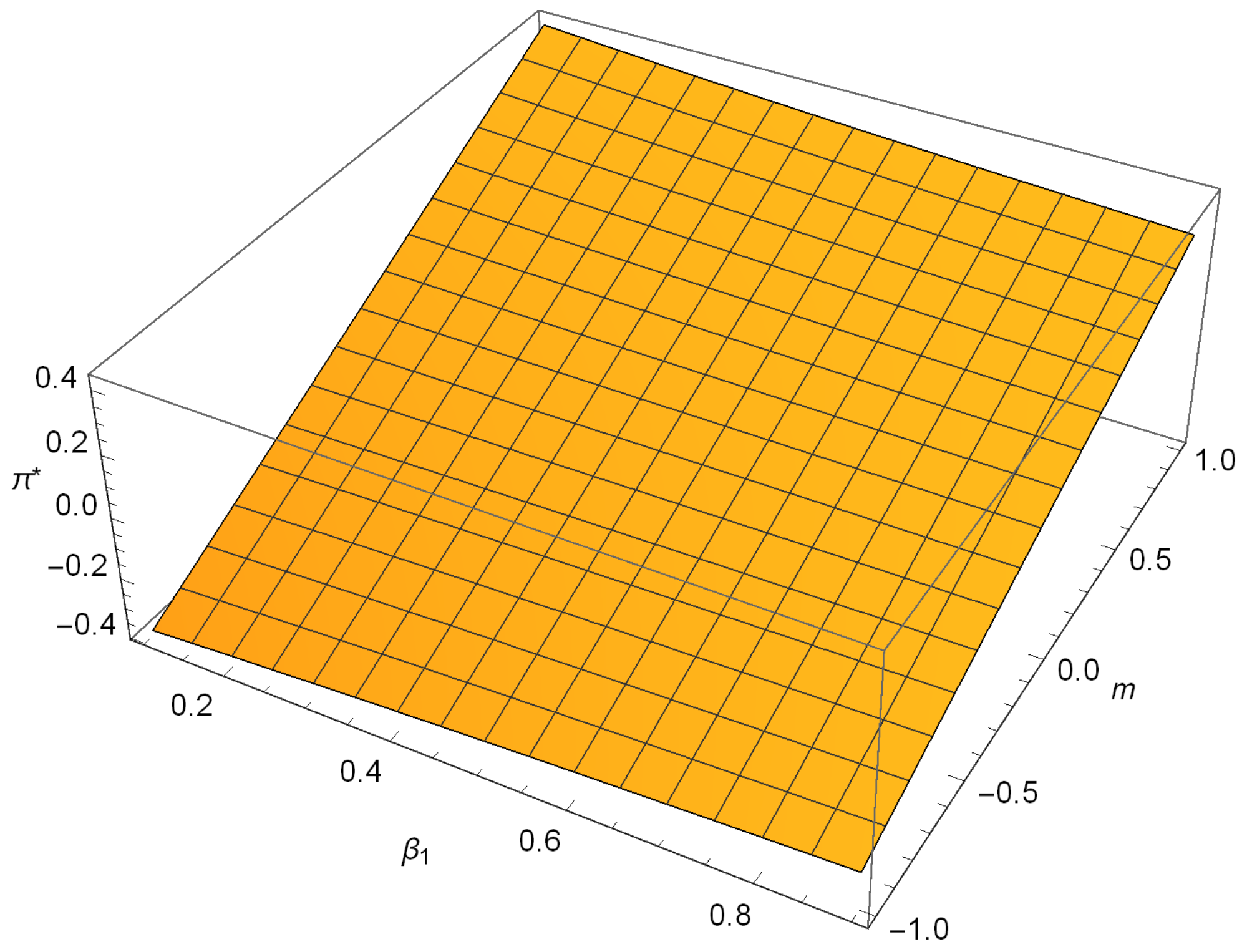
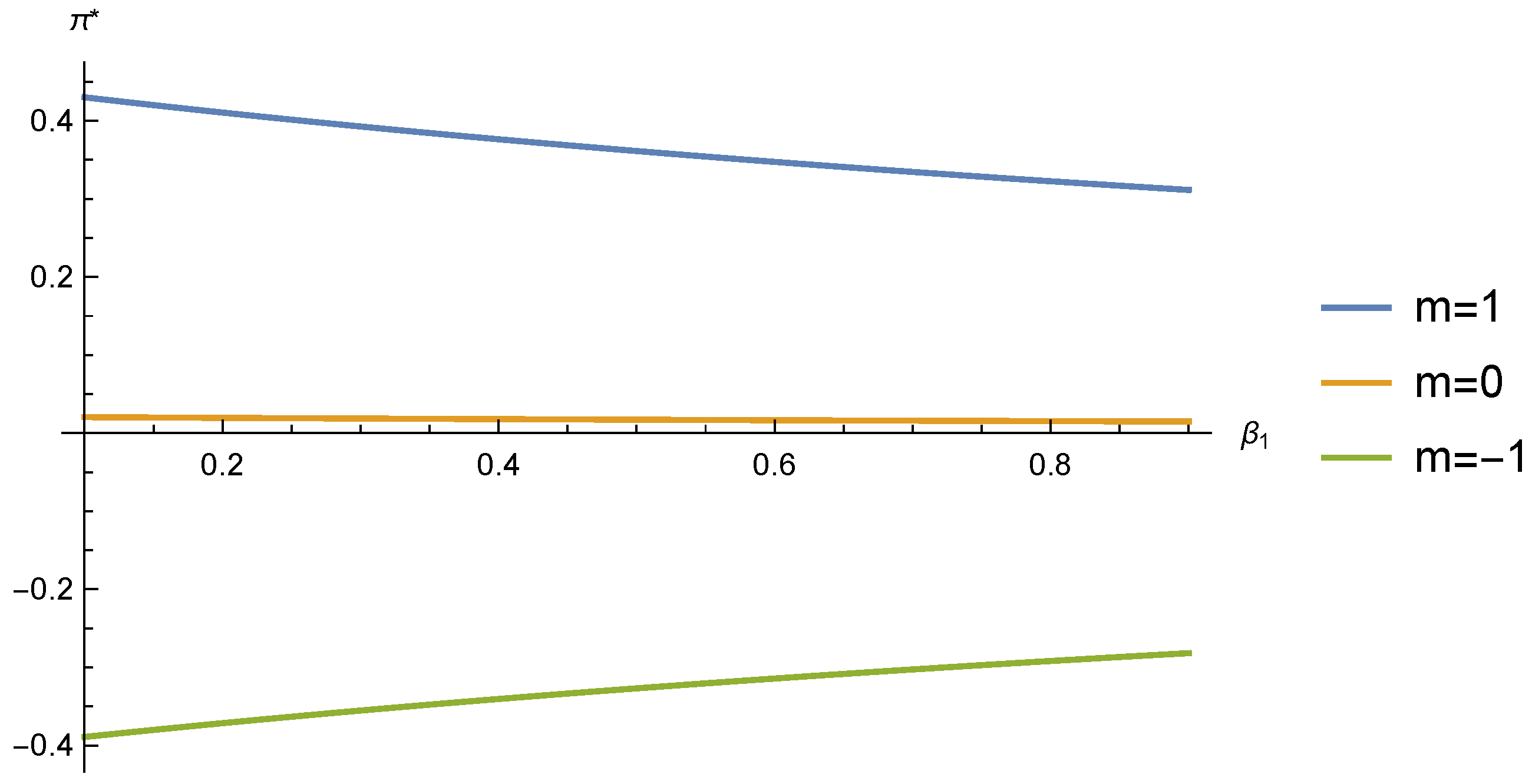
We first explored the impact of β 1 and m on π .  Figure 1 shows the impact of the parameters m and β 1 on the optimal investment policy π when t = 1 . For further clarity, we can see Figure 2. When m = 1 , the investment policy π > 0 decreases with β 1 , meaning the long position is scaled back as ambiguity aversion increases. When m = 1 , the investment policy π < 0 increases with β 1 (i.e., becomes less negative), indicating that the magnitude of the short position is reduced. This behavior reflects the essence of robust control: higher ambiguity aversion leads to smaller absolute exposures, whether long or short, pushing the strategy toward a conservative neutral position. When m = 0 , the exchange rate does not fluctuate much; therefore, as β 1 increases, the insurer’s investment strategy does not change significantly. In the case β 1 = 0 , the distortion parameter is ϕ 1 to zero. This corresponds to full confidence in the reference model P , where the insurer follows the classical non-robust strategy.
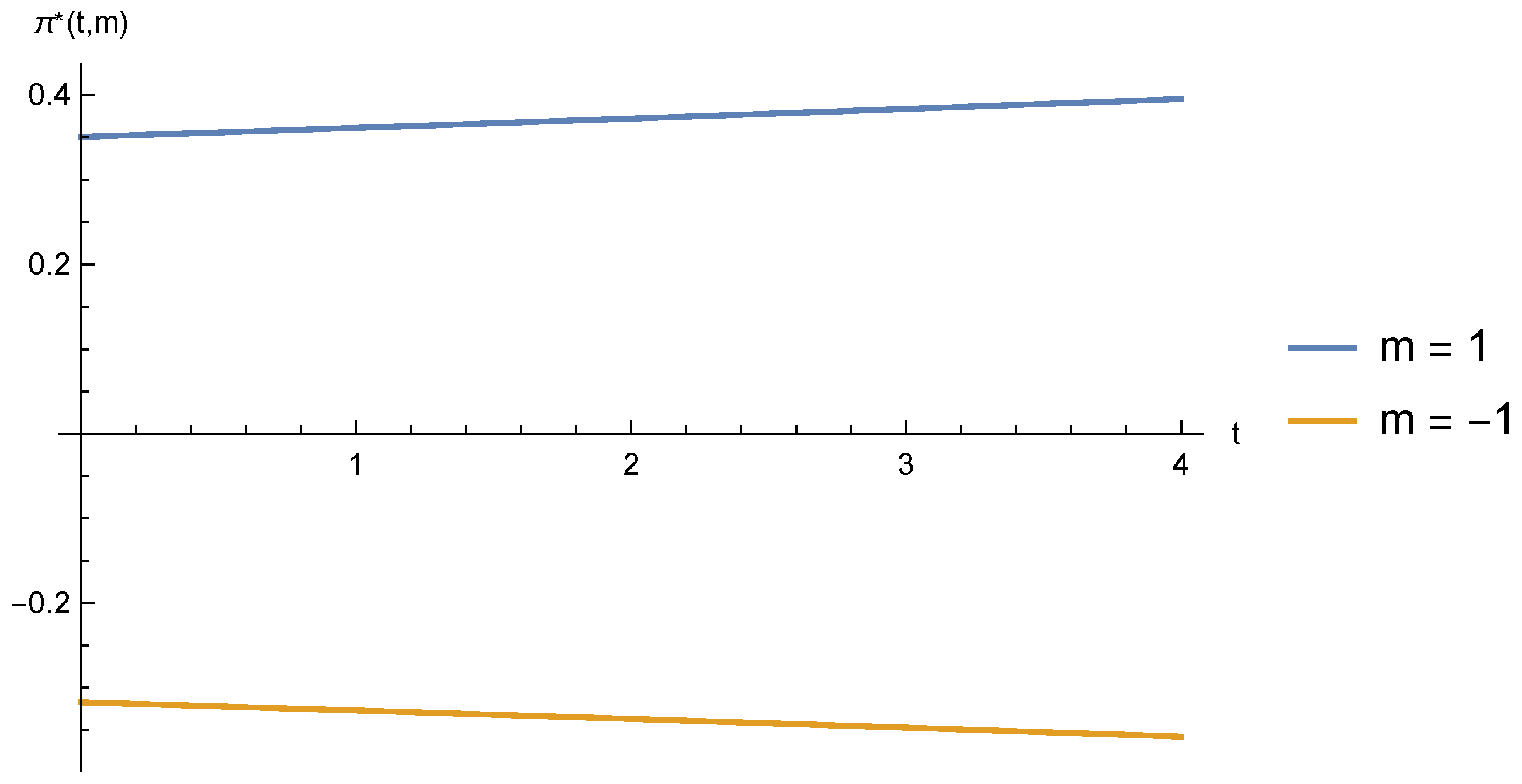
Figure 3 shows the impact of time t on the optimal investment π when m = 1 and m = 1 . When m = 1 , the exchange growth rate will be positive, which means the the market is very confident about the increasing of the exchange rate. In this case, as time t approaches to the terminal time T, the insurer tends to spend more money on the foreign stock market. But when m = 1 , the exchange growth rate will be negative for a while, and as time t approaches to the terminal time T, the ambiguity-averse insurer prefers increasing the amount of short selling.
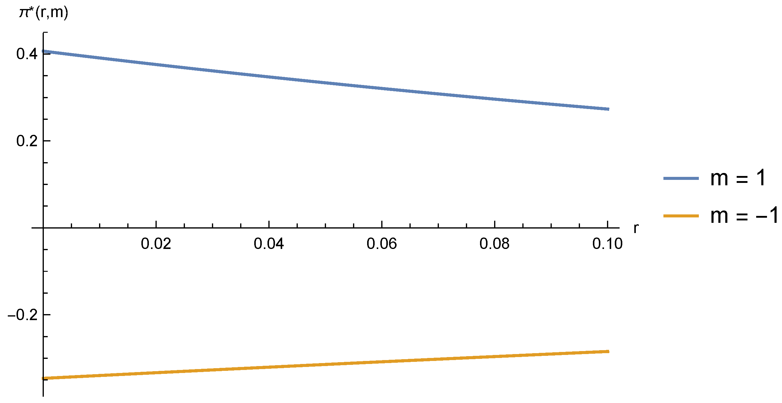
Figure 4 shows the impact of the interest rate r on the optimal investment π when m = 1 and m = 1 at time t = 1 . When m = 1 , the market is confident about the increasing of the exchange rate. A rise in the risk-free rate r makes the domestic risk-free asset relatively more attractive, leading the insurer to reduce its long exposure; hence, π decreases with r. But conversely, when m = 1 , which implies an expected depreciation of the exchange rate, the optimal strategy involves a short position ( π < 0 ). As r increases, the insurer scales back the size of the short position (i.e., | π | decreases) because the higher return on the risk-free asset diminishes the incentive to maintain a large leveraged short position.
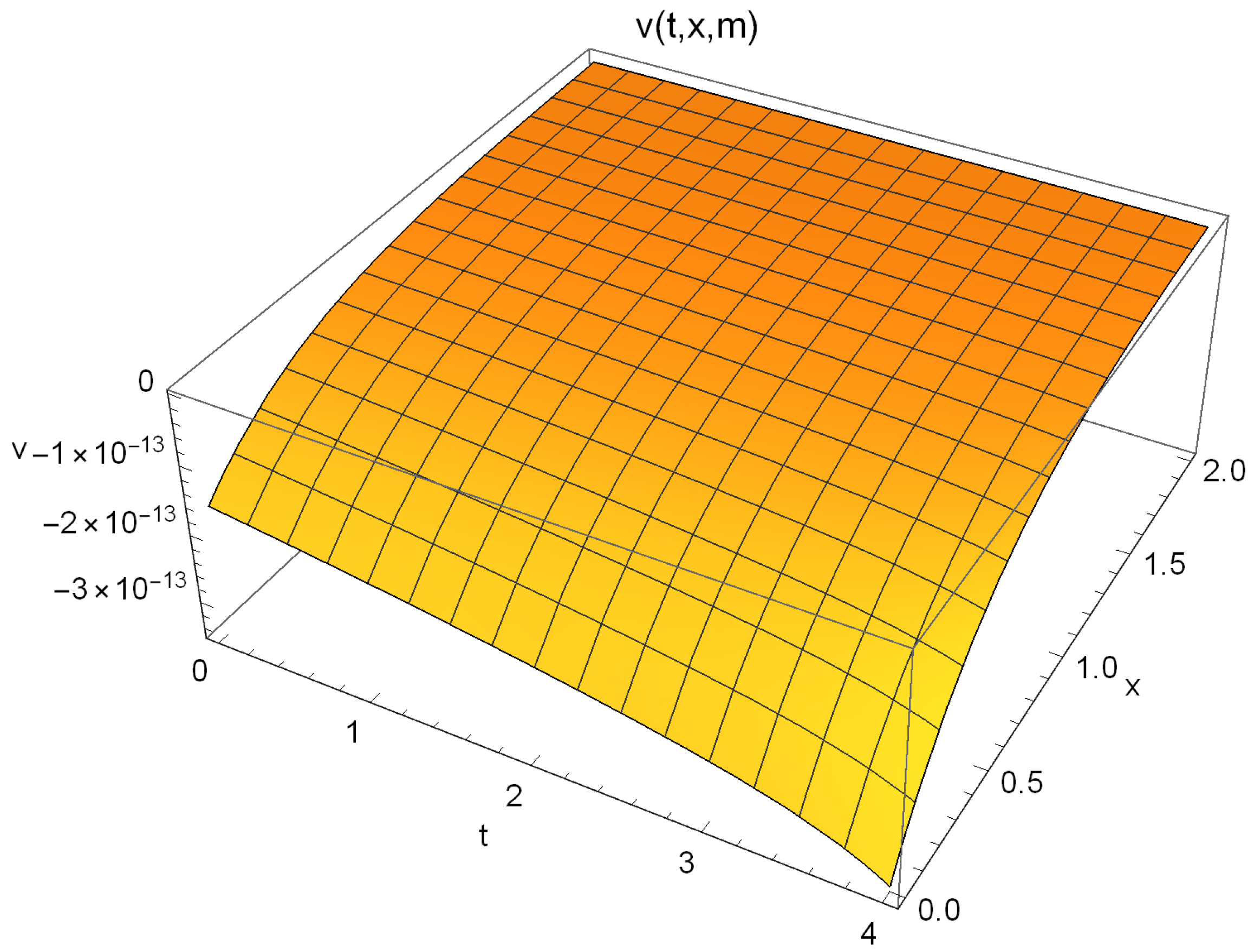
Figure 5 shows the impact of t and x on the optimal value function under fixed m = 1 . The value function exhibits a positive relationship with initial surplus x while declining as time t progresses, a pattern that aligns with fundamental economic intuition. Moreover, the temporal sensitivity of the value function diminishes alongside growth in the insurer’s initial surplus. On the contrary, as the time horizon draws near maturity (i.e., t approaches T), the effect of wealth on the value function becomes increasingly prominent.
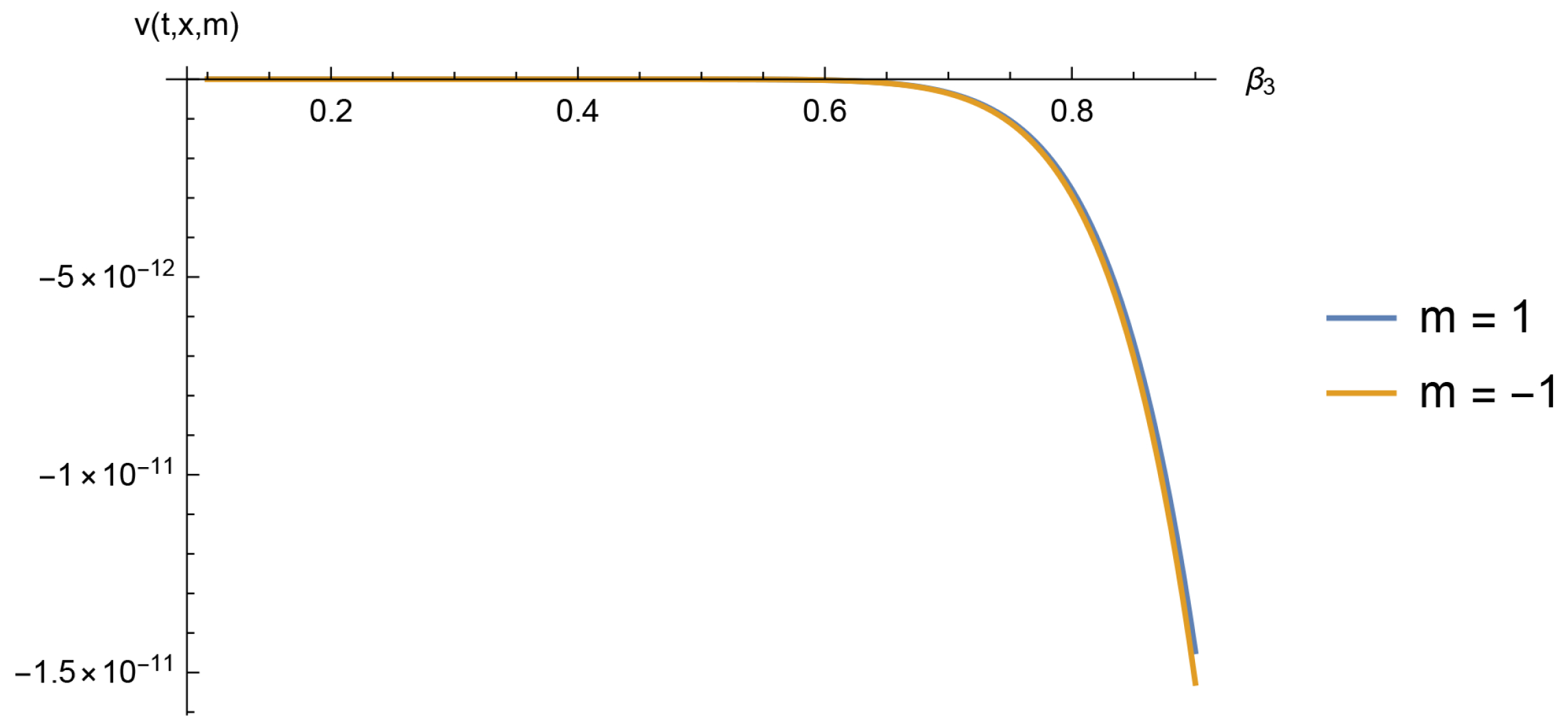
Figure 6 illustrates when t = 1 and x = 1 , and the impact of ambiguity aversion toward claim intensity β 3 on the insurer’s value function under different market signals m = 1 and m = 1 . A higher β 3 consistently lowers the value function in both market states, reflecting the welfare loss from increased doubt about the claim-arrival model. The two curves are nearly indistinguishable, indicating that the damaging effect of claim ambiguity aversion is almost identical regardless of whether the market signal is optimistic m = 1 or pessimistic m = 1 . This near-overlap implies that uncertainty in underwriting impairs firm value to a similar extent in both bull and bear markets. While the value function under m = 1 remains slightly higher—owing to the higher baseline return offered by a positive exchange-rate signal—the marginal deterioration caused by higher β 3 is virtually the same across market regimes. Hence, although a favorable market state provides a higher level of value, it does not alter the sensitivity of the insurer’s welfare to underwriting model uncertainty.
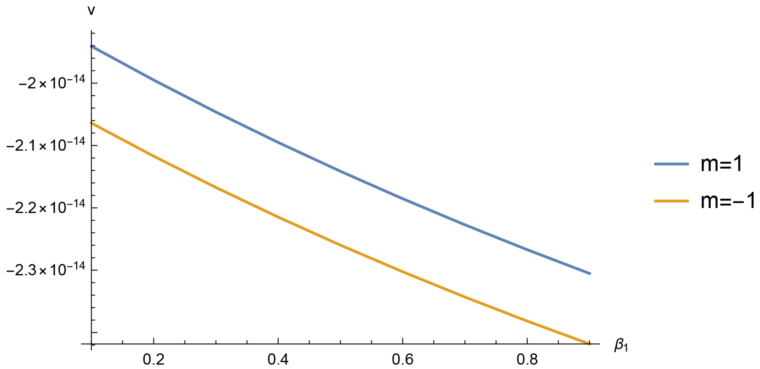
Figure 7 illustrates when t = 1 and x = 1 and how the value function varies with the ambiguity-aversion parameter β 1 for two fixed market states m = 1 and m = 1 . In both cases, the value function decreases monotonically as β 1 rises. A larger β 1 means that the insurer has less confidence in the estimated total excess return of the foreign risky asset; to guard against model misspecification, the insurer adopts a more conservative investment posture, which reduces the utility. For any given β 1 , the value function is higher when m = 1 than when m = 1 because a positive market signal provides a better investment opportunity, even under the same robustness constraint.
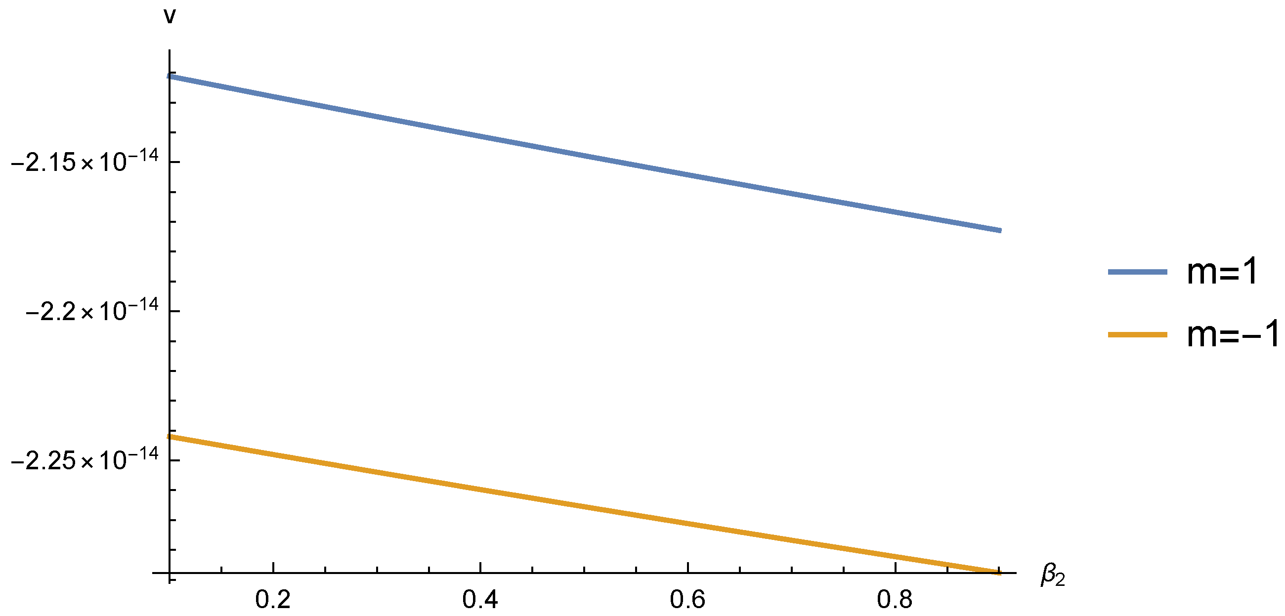
Figure 8 shows, similarly to Figure 7, a monotonic decline of the value function with respect to β 2 when t = 1 and x = 1 . The economic interpretation, however, is different: β 2 captures ambiguity about the mean reverting dynamics of the exchange rate itself. A higher β 2 indicates that the insurer distrusts the predictive power of the Ornstein–Uhlenbeck model for future exchange rate movements. Consequently, the insurer becomes less responsive to the current signal m ( t ) , leading to a more cautious strategy and a lower expected utility.

5. Conclusions

This paper investigated the robust optimal investment problem in the foreign stock market for an ambiguity-averse insurer, modeling the exchange rate as a diffusion process with a stochastic drift that follows an O-U process. By solving the corresponding HJB equation, we derived explicit expressions for the optimal investment policy and the value function. The optimal policy is mainly affected by the risk-free interest rate, the drift of the stock price, the current value of the O-U drift process, the time, the stock volatility, and the ambiguity-aversion coefficient toward stock risk β 1 . Interestingly, it does not depend on the ambiguity regarding the O-U drift dynamics β 2 or the claim process β 3 , although these do affect the value function.
From a policy perspective, the robustness dampens the insurer’s response to the exchange-rate signals derived from the drift process m: a higher ambiguity aversion effectively increases risk aversion, leading to more conservative investment even under strong bullish or bearish signals. These results offer practical insights for insurers managing foreign investments under model uncertainty.


Author Contributions

Methodology, L.T. and X.Z.; validation, Y.T. and L.T.; writing—original draft preparation, Y.T.; writing—review and editing, L.T. and X.Z.; visualization, X.Z.; funding acquisition, L.T. All authors have read and agreed to the published version of the manuscript.

Funding

This work was supported by the National Natural Science Foundation of China (No. 12201104 and 12201174), the Fundamental Research Funds for the Central Universities (No. 2232025D-41).

Data Availability Statement

The data presented in this study were simulated and constructed for analytical purposes. As these are not real-world observational data, they are available from the authors upon request. No public repository hosts these simulated data.

Acknowledgments

We appreciate the anonymous reviewers for their constructive comments, which have significantly improved this manuscript.

Conflicts of Interest

The authors declare no conflicts of interest.

Appendix A

The appendix provides the analysis for the case where W t 1 and W t 2 are two standard Brownian motions, with
E [ d W t 1 d W t 2 ] = ρ d t ,
where ρ ( 1 , 1 ) and ρ 0 . All other model assumptions, objective functions, and solution methodologies remain consistent with the main text.

Appendix A.1. Model Specification Under Correlation

The dynamics of the foreign risky asset price S t f and the exchange rate Q t are as specified in the main text:
d S t f = S t f ( μ f d t + σ f d W t 1 ) , d Q t = Q t ( μ Q + m ( t ) ) d t + σ Q d W t 2 .
With correlation ρ , the insurer’s surplus process must be adjusted. Defining the effective total variance
Σ 2 : = σ f 2 + σ Q 2 + 2 ρ σ f σ Q ,
the surplus dynamics become
d X t = ( p + r X t ) d t + π t μ f + μ Q r + m ( t ) d t + π t Σ 2 d W t i = 1 N t Y i ,
where W t is a standard Brownian motion. Following the same Girsanov transformation as in the main text, under an alternative measure Q , the surplus process is
d X t = ( p + r X t ) d t + π t μ f + μ Q r + m ( t ) γ 1 ( t ) π t Σ 2 λ γ 3 ( t ) μ Y d t + π t Σ 2 d W 1 Q ( t ) R + y N ˜ Q ( d t , d y ) ,
with W 1 Q ( t ) being a standard Brownian motion under Q .

Appendix A.2. Optimal Strategy and Value Function

Following the same solution procedure as in the main text, the generalized optimal investment strategy is obtained as follows:
π = μ f + μ Q r + m e r ( T t ) Σ 2 ( q + β 1 ) .
The corresponding value function maintains the following form:
V ( t , x , m ) = 1 q l ( t ) exp q x e r ( T t ) + K ( t , m ) ,
where l ( t ) is identical to the solution in the main text, and K ( t , m ) = A ( t ) m 2 + B ( t ) m + C ( t ) with the coefficients determined by the ODE system
A ( t ) + 1 2 Σ 2 ( q + β 1 ) + 2 α A ( t ) 2 σ m 2 ( q + β 2 ) A ( t ) 2 = 0 , B ( t ) + μ f + μ Q r Σ 2 ( q + β 1 ) + α B ( t ) 2 σ m 2 ( q + β 2 ) A ( t ) B ( t ) = 0 , C ( t ) + ( μ f + μ Q r ) 2 2 Σ 2 ( q + β 1 ) + σ m 2 A ( t ) 1 2 σ m 2 ( q + β 2 ) B ( t ) 2 = 0 ,
which is subject to A ( T ) = B ( T ) = C ( T ) = 0 .

Appendix A.3. Numerical Analysis

Now, we will examine the sensitivity of both the optimal investment strategy π and the corresponding value function V to the correlation coefficient ρ using the same parameter values as specified in the main text (see Table 1).
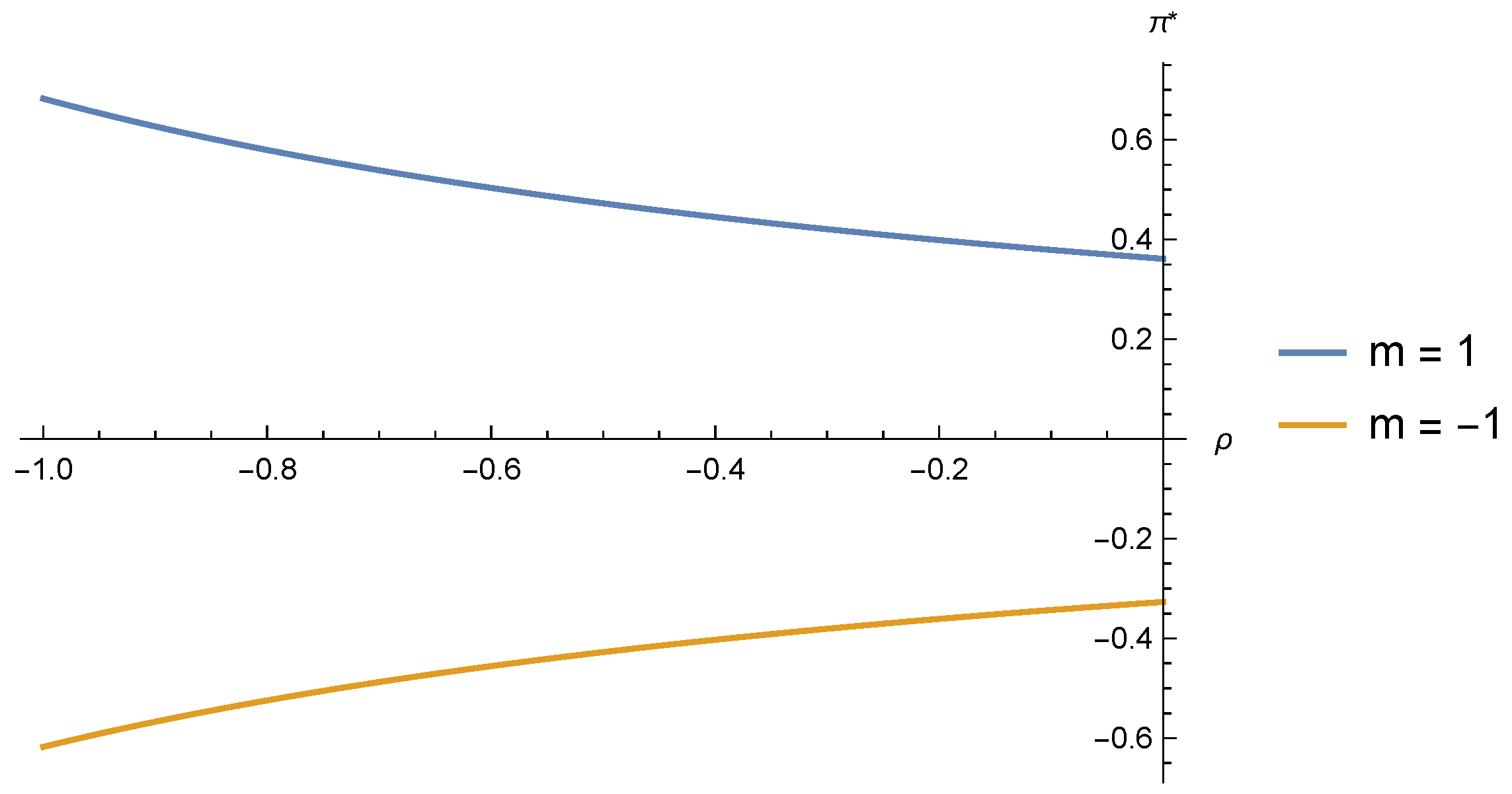
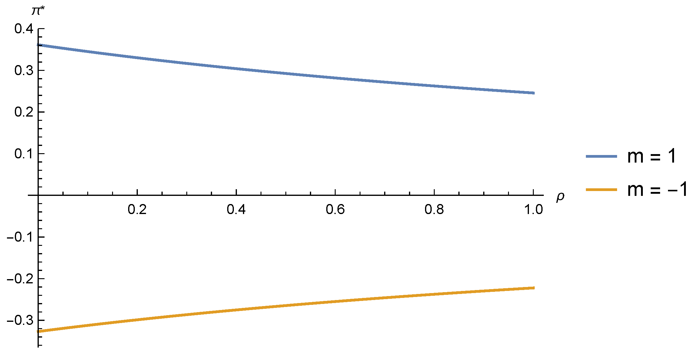
Figure A1 and Figure A2 depict the optimal investment proportion π against the correlation coefficient ρ over the intervals ( 1 , 0 ) and ( 0 , 1 ) for two distinct states represented by m = 1 and m = 1 , respectively. In both figures, | π | decreases monotonically as ρ increases. This trend arises because, in the negative correlation regime (Figure A1), as ρ becomes less negative (moving from —1 toward 0), the beneficial hedging effect weakens. The foreign asset and the exchange rate move less inversely, which increases the combined volatility of the position. Facing this rising uncertainty, the insurer optimally reduces the size of its investment, leading to a smaller | π | . In the positive correlation regime (Figure A2), as ρ increases further (from 0 toward 1), the two risk sources move more in unison, amplifying the portfolio’s total swings. This heightened volatility represents a greater model risk. To safeguard against this, the insurer adopts an even more conservative stance, further scaling down the investment and causing | π | to continue its decline.
Figure A1. The effect of ρ ( 1 , 0 ) on π when m = 1 and m = 1 .
Axioms 15 00030 g0a1
Figure A2. The effect of ρ ( 0 , 1 ) on π when m = 1 and m = 1 .
Axioms 15 00030 g0a2
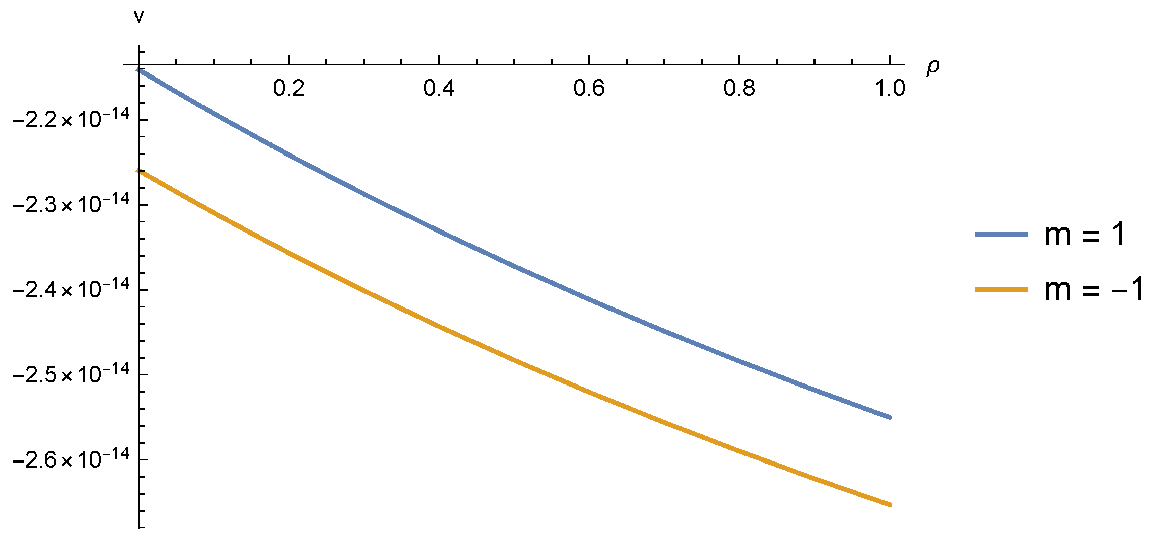
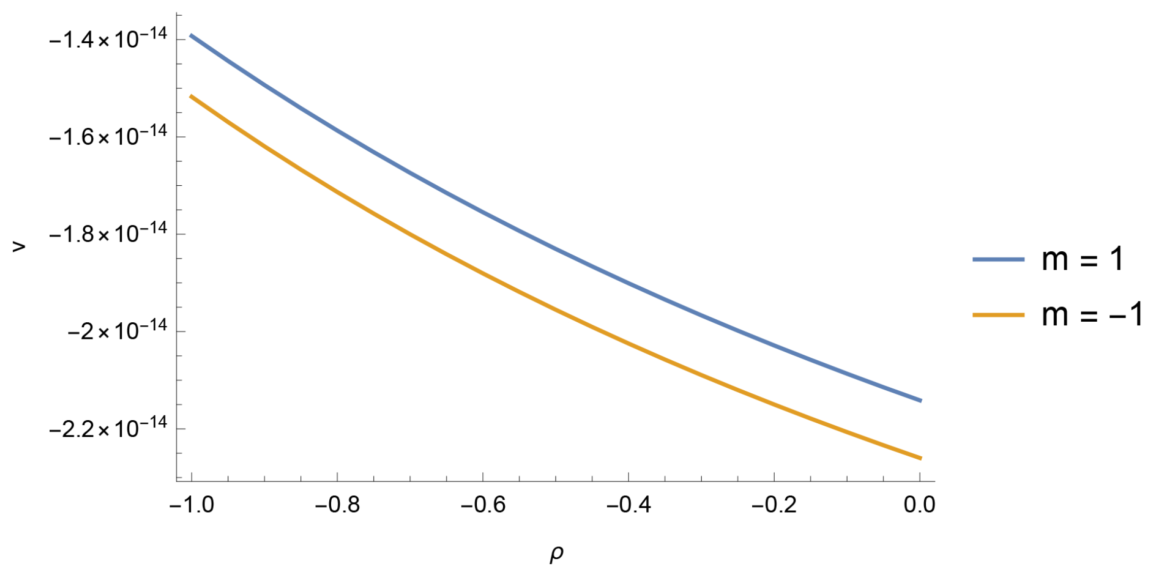
Figure A3 and Figure A4 illustrate the relationship between the value function V and the correlation coefficient ρ for the two market states m = 1 and m = 1 . We can see that the curve corresponding to the favorable state ( m = 1 ) consistently lies above that of the unfavorable state ( m = 1 ), demonstrating that a market with a positive risk premium inherently offers a higher robust welfare guarantee than one requiring a short position. When ρ < 0 (Figure A3), a larger absolute value of ρ leads to a stronger hedging effect of asset fluctuations, lower portfolio volatility, and thus a higher value function; as ρ approaches 0, the hedging effect gradually weakens, portfolio volatility rises, and the value function decreases accordingly. When ρ > 0 (Figure A4), a larger ρ intensifies the synchronous fluctuation of assets, weakens the portfolio diversification effect, increases volatility, and results in a decline in the value function.
Figure A3. The effect of ρ ( 1 , 0 ) on V when m = 1 and m = 1 .
Axioms 15 00030 g0a3
Figure A4. The effect of ρ ( 0 , 1 ) on V when m = 1 and m = 1 .
Axioms 15 00030 g0a4

References

  1. Merton, R.C. Lifetime Portfolio Selection under Uncertainty: The Continuous-Time Case. Rev. Econ. Stat. 1969, 51, 247–257. [Google Scholar] [CrossRef] [Scilit]
  2. Browne, S. Optimal Investment Policies for a Firm with a Random Risk Process: Exponential Utility and Minimizing the Probability of Ruin. Math. Oper. Res. 1995, 20, 937–958. [Google Scholar] [CrossRef] [Scilit]
  3. Guo, C.; Zhuo, X.; Constantinescu, C.; Pamen, O.M. Optimal Reinsurance-Investment Strategy under Risks of Interest Rate, Exchange Rate and Inflation. Methodol. Comput. Appl. Probab. 2018, 20, 1477–1502. [Google Scholar] [CrossRef] [Scilit]
  4. Zhou, Q.; Guo, J. Optimal Investment Strategy for an Insurer in Two Currency Markets. Chin. J. Appl. Probab. Stat. 2025, 41, 1–16. [Google Scholar]
  5. Amin, K.I.; Jarrow, R.A. Pricing Foreign Currency Options under Stochastic Interest Rates. J. Int. Money Financ. 1991, 10, 310–329. [Google Scholar] [CrossRef] [Scilit]
  6. Hansen, L.P.; Sargent, T.J. Robust Control and Model Uncertainty. Am. Econ. Rev. 2001, 91, 60–66. [Google Scholar] [CrossRef] [Scilit]
  7. Maenhout, P.J. Robust Portfolio Rules and Asset Pricing. Rev. Financ. Stud. 2004, 17, 951–983. [Google Scholar] [CrossRef] [Scilit]
  8. Maenhout, P.J. Robust Portfolio Rules and Detection-Error Probabilities for a Mean-Reverting Risk Premium. J. Econ. Theory 2006, 128, 136–163. [Google Scholar] [CrossRef] [Scilit]
  9. Flor, C.R.; Larsen, L.S. Robust Portfolio Choice with Stochastic Interest Rates. Ann. Financ. 2014, 10, 243–265. [Google Scholar] [CrossRef] [Scilit]
  10. Yi, B.; Viens, F.; Li, Z.; Zeng, Y. Robust Optimal Strategies for an Insurer with Reinsurance and Investment under Benchmark and Mean-Variance Criteria. Scand. Actuar. J. 2015, 2015, 725–751. [Google Scholar] [CrossRef] [Scilit]
  11. Li, M.; Deng, Y.; Huang, Y.; Ou, H. Optimal Strategies for an Ambiguity-Averse Insurer under a Jump-Diffusion Model and Defaultable Risk. Math. Probl. Eng. 2020, 2020, 6207805. [Google Scholar] [CrossRef] [Scilit]
  12. Bauerle, N.; Leimcke, G. Robust Optimal Investment and Reinsurance Problems with Learning. Scand. Actuar. J. 2021, 2021, 82–109. [Google Scholar] [CrossRef] [Scilit]
  13. Wang, N.; Siu, T.K.; Fan, K. Robust Reinsurance and Investment Strategies under Principal-Agent Framework. Ann. Oper. Res. 2024, 336, 981–1011. [Google Scholar] [CrossRef] [Scilit]
  14. Feng, Y.; Siu, T.K.; Zhu, J. Optimal Payout Strategies When Bruno de Finetti Meets Model Uncertainty. Insur. Math. Econ. 2024, 116, 148–164. [Google Scholar] [CrossRef] [Scilit]
  15. Guan, G.; Wang, X. Time-Consistent Reinsurance and Investment Strategies for an AAI under Smooth Ambiguity Utility. Scand. Actuar. J. 2020, 2020, 677–699. [Google Scholar] [CrossRef] [Scilit]
  16. Polak, P.; Ulrych, U. Dynamic currency hedging with non-Gaussianity and ambiguity. Quant. Financ. 2024, 24, 305–327. [Google Scholar] [CrossRef] [Scilit]
  17. Schmidli, H. On Minimizing the Ruin Probability by Investment and Reinsurance. Ann. Appl. Probab. 2002, 12, 890–907. [Google Scholar] [CrossRef] [Scilit]
  18. Pressacco, F.; Serafini, P.; Ziani, L. Mean-Variance Efficient Strategies in Proportional Reinsurance under Group Correlation in a Gaussian Framework. Eur. Actuar. J. 2011, 1, 433–454. [Google Scholar] [CrossRef] [Scilit]
  19. Pham, H. Continuous-Time Stochastic Control and Optimization with Financial Applications; Springer Science & Business Media: Berlin, Germany, 2009; Volume 61. [Google Scholar]
  20. Schmidli, H. Stochastic Control in Insurance; Springer Science & Business Media: Berlin, Germany, 2007. [Google Scholar]
  21. Rishel, R. Optimal Portfolio Management with Partial Observations and Power Utility Function. In Stochastic Analysis, Control, Optimization and Applications: A Volume in Honor of W.H. Fleming; McEneaney, W.M., Yin, G.G., Zhang, Q., Eds.; Birkhäuser: Boston, MA, USA, 1999; pp. 605–619. [Google Scholar]
  22. Liang, Z.; Yuen, K.C. Optimal Dynamic Reinsurance with Dependent Risks: Variance Premium Principle. Scand. Actuar. J. 2016, 2016, 18–36. [Google Scholar] [CrossRef] [Scilit]
  23. Gerber, H. An Introduction to Mathematical Risk Theory; S.S. Huebner Foundation for Insurance Education, Wharton School, University of Pennsylvania: Philadelphia, PA, USA, 1979. [Google Scholar]
  24. Li, D.; Zeng, Y.; Yang, H. Robust Optimal Excess-of-Loss Reinsurance and Investment Strategy for an Insurer in a Model with Jumps. Scand. Actuar. J. 2018, 2018, 145–171. [Google Scholar] [CrossRef] [Scilit]
  25. Zheng, X.; Zhou, J.; Sun, Z. Robust Optimal Portfolio and Proportional Reinsurance for an Insurer under a CEV Model. Insur. Math. Econ. 2016, 67, 77–87. [Google Scholar] [CrossRef] [Scilit]
  26. Anderson, E.W.; Hansen, L.P.; Sargent, T.J. A Quartet of Semigroups for Model Specification, Robustness, Prices of Risk, and Model Detection. J. Eur. Econ. Assoc. 2003, 1, 68–123. [Google Scholar] [CrossRef] [Scilit]
  27. Branger, N.; Larsen, L.S. Robust Portfolio Choice with Uncertainty about Jump and Diffusion Risk. J. Bank. Financ. 2013, 37, 5036–5047. [Google Scholar] [CrossRef] [Scilit]
  28. Mataramvura, S.; Øksendal, B. Risk Minimizing Portfolios and HJBI Equations for Stochastic Differential Games. Stochastics 2008, 80, 317–337. [Google Scholar] [CrossRef] [Scilit]
  29. Yong, J.M.; Zhou, X.Y. Stochastic Controls: Hamiltonian Systems and HJB Equations; Springer: New York, NY, USA, 1999. [Google Scholar]
  30. Hale, J.K. Ordinary Differential Equations, 2nd ed.; Wiley-Interscience: New York, NY, USA, 1980. [Google Scholar]
Figure 1. The effect of m and β 1 on π when time t = 1 .
Axioms 15 00030 g001
Figure 2. The effect of β 1 on π when m = 1 , m = 0 , and m = 1 .
Axioms 15 00030 g002
Figure 3. The effect of time t on π when m = 1 and m = 1 .
Axioms 15 00030 g003
Figure 4. The effect of interest rate r on π when m = 1 and m = 1 at time t = 1 .
Axioms 15 00030 g004
Figure 5. The effect of t and x on V when m = 1 .
Axioms 15 00030 g005
Figure 6. The effect of β 3 on V when m = 1 and m = 1 at time t = 1 .
Axioms 15 00030 g006
Figure 7. The effect of β 1 on V when m = 1 and m = 1 at time t = 1 .
Axioms 15 00030 g007
Figure 8. The effect of β 2 on V when m = 1 and m = 1 at time t = 1 .
Axioms 15 00030 g008
Table 1. The parameters of model in numerical examples.
λ θ λ Y pr α μ f σ f μ Q σ m Tq β 1 β 2 β 3 σ Q t
20.321.30.03—10.080.2501420.50.40.611
Disclaimer/Publisher’s Note: The statements, opinions and data contained in all publications are solely those of the individual author(s) and contributor(s) and not of MDPI and/or the editor(s). MDPI and/or the editor(s) disclaim responsibility for any injury to people or property resulting from any ideas, methods, instructions or products referred to in the content.