Element-Oriented Construction Methods for Nullnorms on Bounded Lattices

Abstract

Nullnorms are aggregation functions with an annihilator and are generalizations of t-norms and t-conorms. After the introduction of the concept of nullnorms on bounded lattices by Karaçal et al., the studies on their construction methods in such structures have been initiated. Following the paper of Karaçal and Şanlı, in which proposed element-based construction methods for t-norms and t-conorms on bounded lattices, a natural research question emerged: Are there any element-based construction methods for nullnorms on a bounded lattice L? In this paper, we address this question and propose construction methods for nullnorms with an annihilator element $k\in L\setminus \{0,1\}$, depending on an element $\eta \in L\setminus \{0,k,1\}$, by examining the relationship between $\eta$ and k. The proposed methods are compared with some existing approaches in the literature and are shown to be distinct. These theoretical findings are further supported with illustrative examples.

1. Introduction

Nullnorms and t-operators were first introduced on the unit interval by Calvo et al. [1] and Mas et al. [2], and it was proven that they are equivalent on the unit interval in [3]. These operators are crucial in a wide range of fields, including fuzzy logic, fuzzy quantifiers, decision making, expert systems, and neural networks. Nullnorms are generalizations of t-norms and t-conorms since they allow the annihilator element k to be chosen from anywhere on the unit interval, and they are t-norms when $k=0$ and t-conorms when $k=1$. Nullnorms on the unit interval were discussed in many papers [4,5,6].

Karaçal et al. [7] introduced the concept of nullnorms with an annihilator element $k\in L\setminus \{0,1\}$ on the bounded lattice L based on the fact that a t-norm (or t-conorm) always exists on any bounded lattice L. While nullnorms are widely discussed in the literature [8,9,10,11,12,13,14,15,16,17], element-oriented construction methods for nullnorms on bounded lattices remain underexplored. This paper addresses this gap by proposing such methods for nullnorms on bounded lattices.

The paper is structured as follows. In Section 2, we review the concepts of bounded lattices, t-norms, t-conorms and nullnorms on bounded lattices. Section 3 presents the main results including the new element-based construction methods for nullnorms on a bounded lattice L based on the element $\eta$ by elaborating $\eta \in I_k$, $\eta \in (k,1)$ or $\eta \in (0,k)$. To exemplify these construction methods, we present several examples. Moreover, we demonstrate through the examples that our new construction methods differ from previously proposed methods.

2. Notations, Definitions and a Review of Previous Results

This section reviews related concepts.

Definition 1

([18]). The elements p and q in a bounded lattice L are called comparable if $p\le q$ or $q\le p$; otherwise, they are called incomparable and notated by $p\left|\right|q$, and also the set $I_a=\{p\in L:p|\left|a\right\}$ is defined.

Definition 2

([19]). A triangular norm (conorm) T (S) on a bounded lattice L, shortly t-norm (t-conorm), is an $L^2\to L$ increasing function satisfying commutativity, associativity and having a neutral element 1 (0).

Definition 3

([7]). A nullnorm $F:L^2\to L$ is a commutative, associative, non-decreasing function having an element $k\in L$ such that $F(p,0)=p$ for all $p\in [0,k]$, $F(p,1)=p$ for all $p\in [k,1]$, which is an annihilator (zero element) for F.

We recommend refs. [7,9,14,17] for more details about nullnorms on bounded lattices.

3. Element-Based Construction Methods of Nullnorms on Bounded Lattices

In this section, keeping in mind the paper of Karaçal and Şanlı in [20], in which they presented an element-based triangular norm construction, we introduce three nullnorms construction methods on a bounded lattice L in Theorems 1, 3 and 4, based on an arbitrary element $\eta \notin \{0,k,1\}$. Then, we compare our methods with those methods already in the literature and highlight the differences between our approach and the recalled ones. Finally, we provide some illustrative examples.

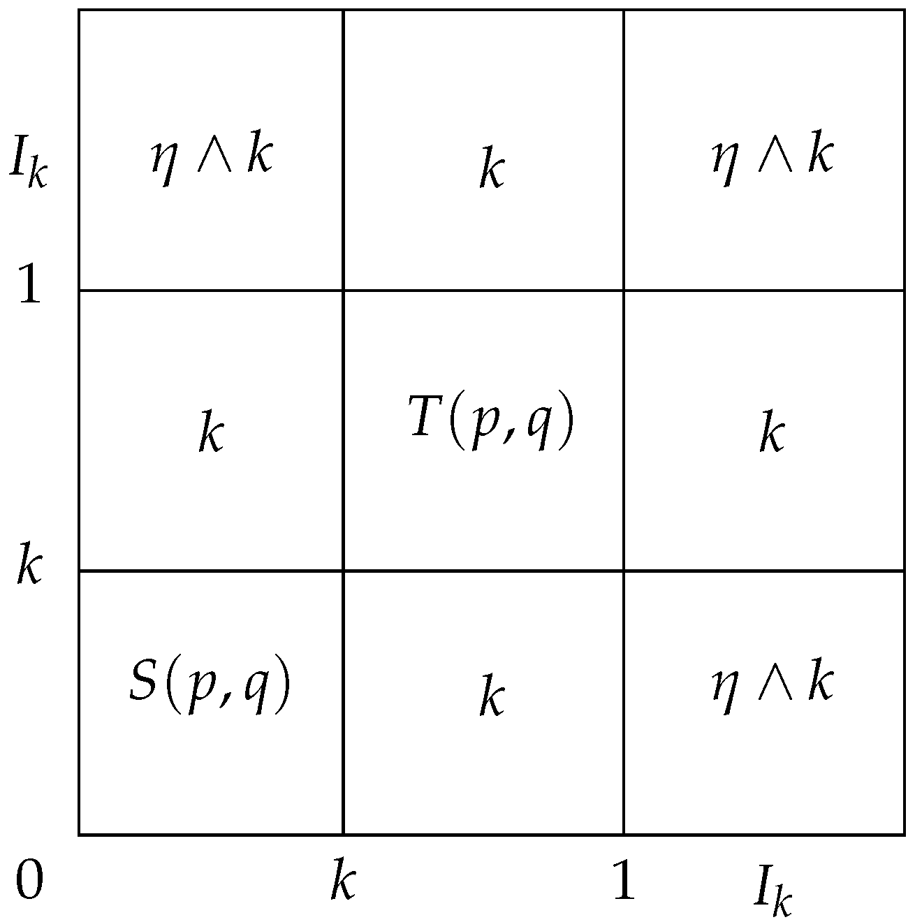
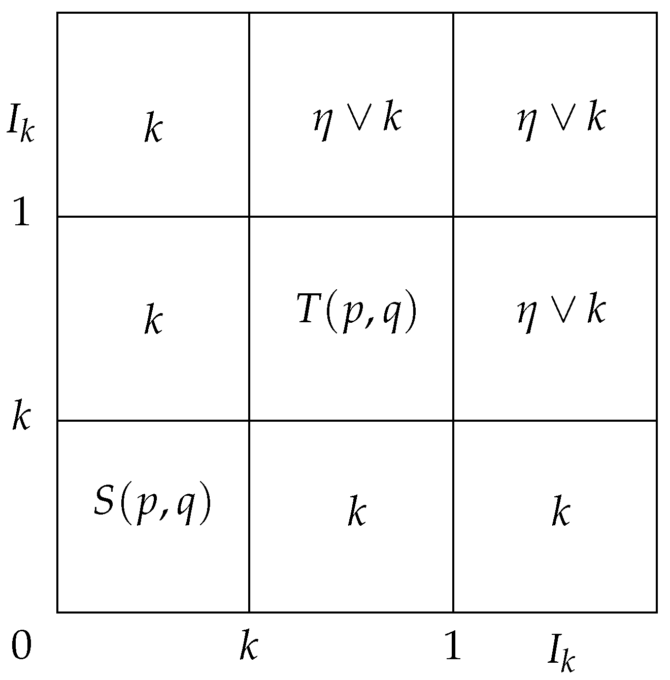
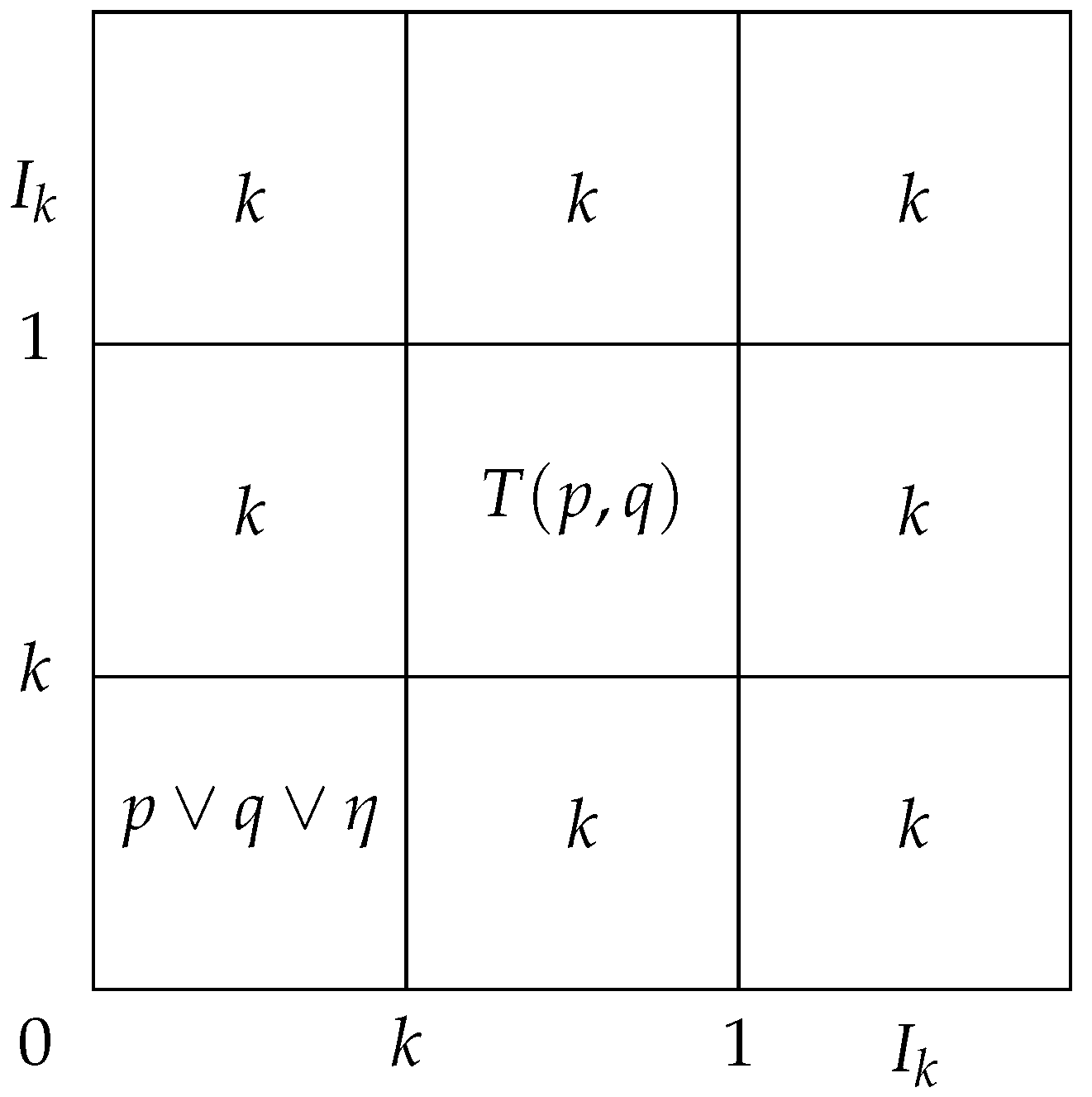
In the following theorem, Formula (1) produces a nullnorm on the bounded lattice L satisfying $p<q$ for all $p\in [0,k),q\in I_k$ when $\eta \in I_k$ is a fixed element. We can obtain the following nullnorm construction method by considering the t-conorm S on $[0,k]$ satisfying $S(\eta \wedge k,\eta \wedge k)=\eta \wedge k$ and the t-norm T on $[k,1]$.

Theorem 1.

Let $k\in L\setminus \{0,1\}$ be an element of bounded lattice L, $\eta \in I_k$, S be a t-conorm on $[0,k]$ satisfying $S(\eta \wedge k,\eta \wedge k)=\eta \wedge k$ and T be a t-norm on $[k,1]$. If $p<q$ for all $p\in [0,k),q\in I_k$, then the function $Z_1:L^2\to L$ defined by

$$Z_1(p,q)=\left\{\begin{array}{cc}S(p,q)\hfill & if(p,q)\in {[0,k)}^2,\hfill \\ T(p,q)\hfill & if(p,q)\in {[k,1]}^2,\hfill \\ \eta \wedge k\hfill & if(p,q)\in ([0,k)\cup I_k)\times I_k\cup I_k\times [0,k),\hfill \\ k\hfill & otherwise,\hfill \end{array}\right.$$

(1)

is a nullnorm on L with the annihilator element k.

Proof. 

By the definition of the function $Z_1$, it is clear that $Z_1$ is a commutative function with the annihilator element k. Now, in the following, let us check that the monotonicity and associativity hold.

(i)

Monotonicity: Let us show that for all elements $p,q\in L$ with $p\le q$, $Z_1(p,r)\le Z_1(q,r)$ for all $r\in L$. If p and q are both elements of $[0,k)$ or $\left\{k\right\}$ or $(k,1]$ or $I_k$, $Z_1(p,r)\le Z_1(q,r)$ is always satisfied for all $r\in L$ since $p\le q$. Then, the proof then considers all of the remaining cases.

1.

Let $p\in [0,k)$.

(1.1)

$q=k$ $(q\in (k,1\left]\right)$,

(1.1.1)

If $r\in [0,k)$, then $Z_1(p,r)=S(p,r)\le k=Z_1(q,r).$

(1.1.2)

If $r\in [k,1]$, then $Z_1(p,r)=k(\le T(q,r))=Z_1(q,r).$

(1.1.3)

If $r\in I_k$, then $Z_1(p,r)=\eta \wedge k\le k=Z_1(q,r).$

(1.2)

$q\in I_k$,

(1.2.1)

If $r\in [0,k)$, then $Z_1(p,r)=S(p,r)\le \eta \wedge k=Z_1(q,r).$

(1.2.2)

If $r\in [k,1]$, then $Z_1(p,r)=k=Z_1(q,r).$

(1.2.3)

If $r\in I_k$, then $Z_1(p,r)=\eta \wedge k=Z_1(q,r).$

2.

Let $p=k$,

(2.1)

$q\in (k,1]$,

(2.1.1)

If $r\in [0,k]\cup I_k$, then $Z_1(p,r)=k=Z_1(q,r).$

(2.1.2)

If $r\in [k,1]$, then $Z_1(p,r)=k\le T(q,r)=Z_1(q,r).$

3.

Let $p\in I_k$,

(3.1)

$q\in (k,1]$,

(3.1.1)

If $r\in [0,k)\cup I_k$, then $Z_1(p,r)=\eta \wedge k\le k=Z_1(q,r).$

(3.1.2)

If $r\in [k,1]$, then $Z_1(p,r)=k\le T(q,r)=Z_1(q,r).$

(ii)

Associativity: We demonstrate that $Z_1(p,Z_1(q,r))=Z_1(Z_1(p,q),r)$ for all $p,q,r\in L$. If $p=k$, the equality is satisfied; therefore, they are omitted. Again, taking that $Z_1$ is commutative into account for that proof, we consider all of the remaining cases as follows.

1.

Let $p\in [0,k)$.

(1.1)

$q\in [0,k)$,

(1.1.1)

If $r\in [0,k)$, then $Z_1(p,Z_1(q,r))=Z_1(p,S(q,r))=S(p,S(q,r))=S(S(p,q),r)=Z_1(S(p,q),r)=Z_1(Z_1(p,q),r).$

(1.1.2)

If $r\in (k,1]$, then $Z_1(p,Z_1(q,r))=Z_1(p,k)=k=Z_1(S(p,q),r)=Z_1(Z_1(p,q),r).$

(1.1.3)

If $r\in I_k$, then $Z_1(p,Z_1(q,r))=Z_1(p,\eta \wedge k)=S(p,\eta \wedge k)=\eta \wedge k=Z_1(S(p,q),r)=Z_1(Z_1(p,q),r).$

(1.2)

$q\in (k,1]$,

(1.2.1)

If $r\in [0,k)\cup I_k$, then $Z_1(p,Z_1(q,r))=Z_1(p,k)=k=Z_1(k,r)=Z_1(Z_1(p,q),r).$

(1.2.2)

If $r\in (k,1]$, then $Z_1(p,Z_1(q,r))=Z_1(p,T(q,r))=k=Z_1(k,r)=Z_1(Z_1(p,q),r).$

(1.3)

$q\in I_k$,

(1.3.1)

If $r\in [0,k)$, then $Z_1(p,Z_1(q,r))=Z_1(p,\eta \wedge k)=S(p,\eta \wedge k)=\eta \wedge k=S(\eta \wedge k,r)=Z_1(\eta \wedge k,r)=Z_1(Z_1(p,q),r).$

(1.3.2)

If $r\in (k,1]$, then $Z_1(p,Z_1(q,r))=Z_1(p,k)=k=Z_1(\eta \wedge k,r)=Z_1(Z_1(p,q),r).$

(1.3.3)

If $r\in I_k$, then $Z_1(p,Z_1(q,r))=Z_1(p,\eta \wedge k)=S(p,\eta \wedge k)=\eta \wedge k=Z_1(\eta \wedge k,r)=Z_1(Z_1(p,q),r).$

2.

Let $p\in (k,1]$.

(2.1)

$y\in [0,k)$,

(2.1.1)

If $r\in (k,1]$, then $Z_1(p,Z_1(q,r))=Z_1(p,k)=k=Z_1(k,r)=Z_1(Z_1(p,q),r).$

(2.1.2)

If $r\in I_k$, then $Z_1(p,Z_1(q,r))=Z_1(p,\eta \wedge k)=k=Z_1(k,r)=Z_1(Z_1(p,q),r).$

(2.2)

$q\in (k,1]$,

(2.2.1)

If $r\in I_k$, then $Z_1(p,Z_1(q,r))=Z_1(p,k)=k=Z_1(T(p,q),r)=Z_1(Z_1(p,q),r).$

(2.2.2)

If $r\in (k,1]$, then $Z_1(p,Z_1(q,r))=Z_1(p,T(q,r))=T(p,T(q,r)=T(T(p,q),r)=Z_1(T(p,q),r)=Z_1(Z_1(p,q),r).$

(2.3)

$q\in I_k$,

(2.3.1)

If $r\in I_k$, then $Z_1(p,Z_1(q,r))=Z_1(p,\eta \wedge k)=k=Z_1(k,r)=Z_1(Z_1(p,q),r).$

(2.3.2)

If $r\in (k,1]$, then $Z_1(p,Z_1(q,r))=Z_1(p,k)=k=Z_1(k,r)=Z_1(Z_1(p,q),r).$

3.

Let $p\in I_k$.

(3.1)

$q\in [0,k)$,

(3.1.1)

If $r\in I_k$, then $Z_1(p,Z_1(q,r))=Z_1(p,\eta \wedge k)=\eta \wedge k=Z_1(\eta \wedge k,r)=Z_1(Z_1(p,q),r).$

(3.2)

$q\in (k,1]$,

(3.2.1)

If $r\in I_k$, then $Z_1(p,Z_1(q,r))=Z_1(p,k)=k=Z_1(k,r)=Z_1(Z_1(p,q),r).$

(3.3)

$q\in I_k$,

(3.3.1)

If $r\in I_k$, then $Z_1(p,Z_1(q,r))=Z_1(p,\eta \wedge k)=\eta \wedge k=Z_1(\eta \wedge k,r)=Z_1(Z_1(p,q),r).$

Therefore, $Z_1$ is a nullnorm on L, whose annihilator element is k. □

The structure of the nullnorm $Z_1$ given in Formula (1) is summarized in Figure 1.

To illustrate Theorem 1, we provide the following example.

Example 1.

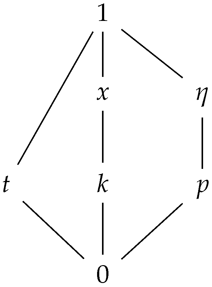
Let us consider $(L_1=\{0,k,p,t,x,\eta ,1\},\le )$ as shown in Figure 2; then, the nullnorm $Z_1$ on $L_1$ with annihilator element k is calculated as in

Table 1. The nullnorm $Z_1$ induced by Formula (1) in Theorem 1.

$Z_1$	0	k	p	t	x	$\eta$	1
0	0	k	0	0	k	0	k
k	k	k	k	k	k	k	k
p	0	k	0	0	k	0	0
t	0	k	0	0	k	0	k
x	k	k	k	k	k	k	x
$\eta$	0	k	0	0	k	0	0
1	k	k	0	k	x	0	1

, when $T=T_D$ and $S=S_D$.

By considering $T=T_{\wedge }$ and $S=S_{\vee }$ in Theorem 1, the following Corollary 1 is obtained.

Corollary 1.

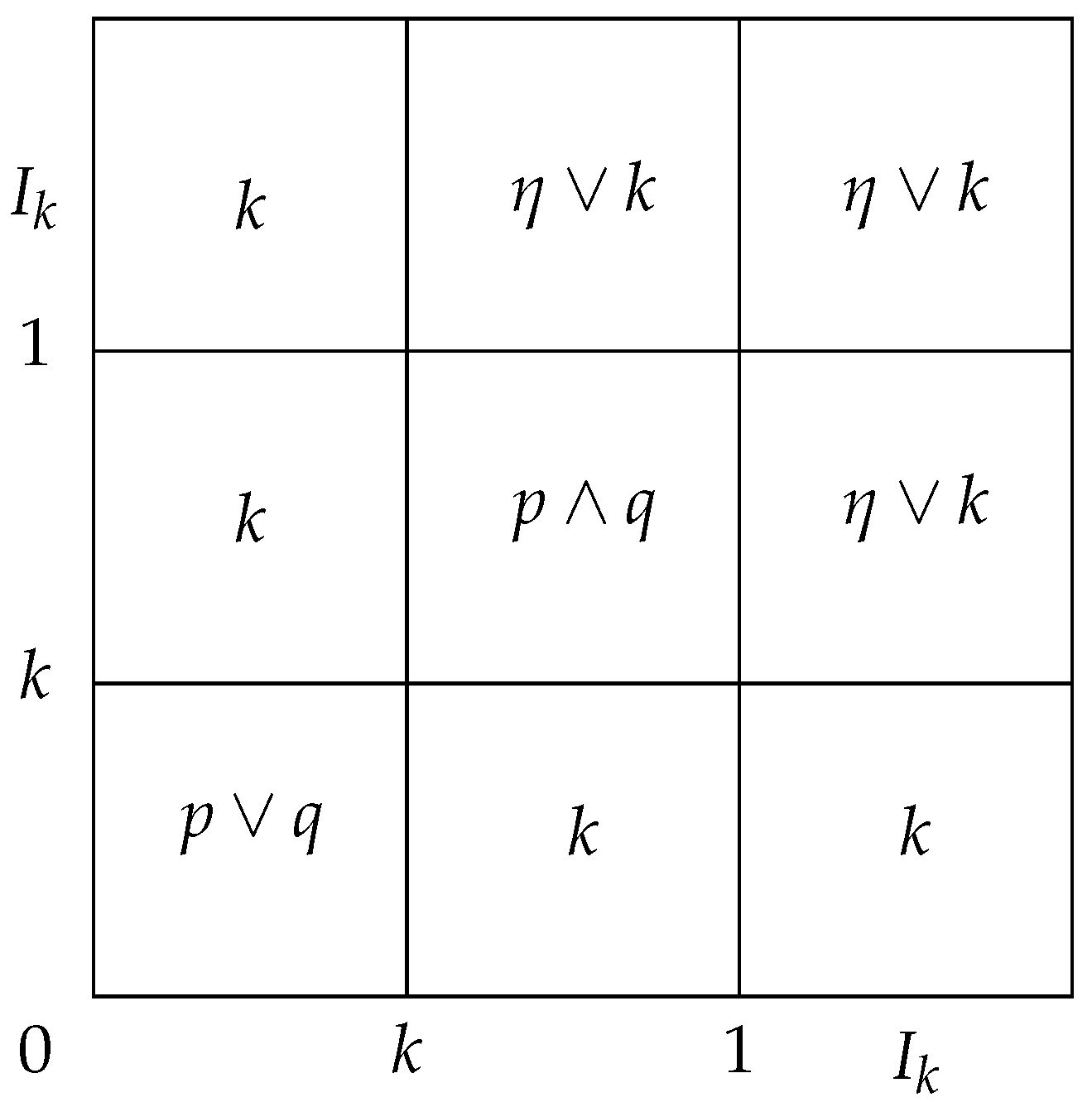
Let $k\in L\setminus \{0,1\}$ be an element of bounded lattice L and $\eta \in I_k$. If $p<q$ for all $p\in [0,k),q\in I_k$, then the function $Z^{\ast 1}:L^2\to L$ defined by

$$Z^{\ast 1}(p,q)=\left\{\begin{array}{cc}p\vee q\hfill & if(p,q)\in {[0,k)}^2,\hfill \\ p\wedge q\hfill & if(p,q)\in {[k,1]}^2,\hfill \\ \eta \wedge k\hfill & if(p,q)\in ([0,k)\cup I_k)\times I_k\cup I_k\times [0,k),\hfill \\ k\hfill & otherwise,\hfill \end{array}\right.$$

(2)

is a nullnorm on L with the annihilator element k.

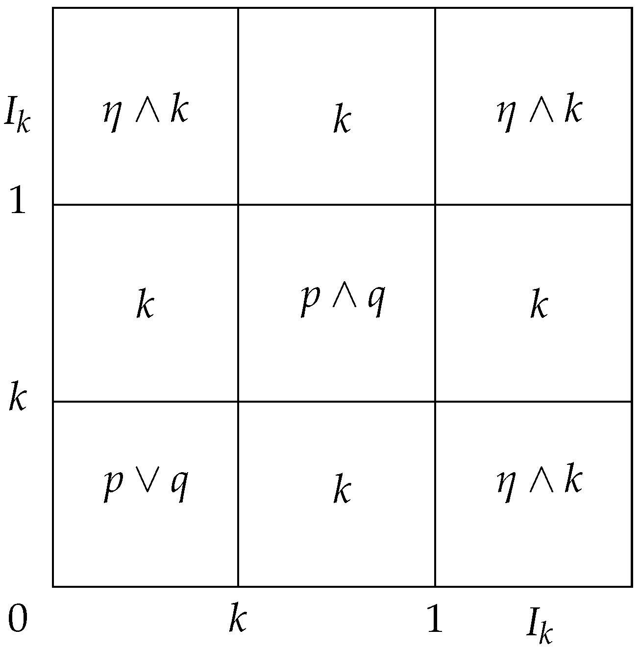
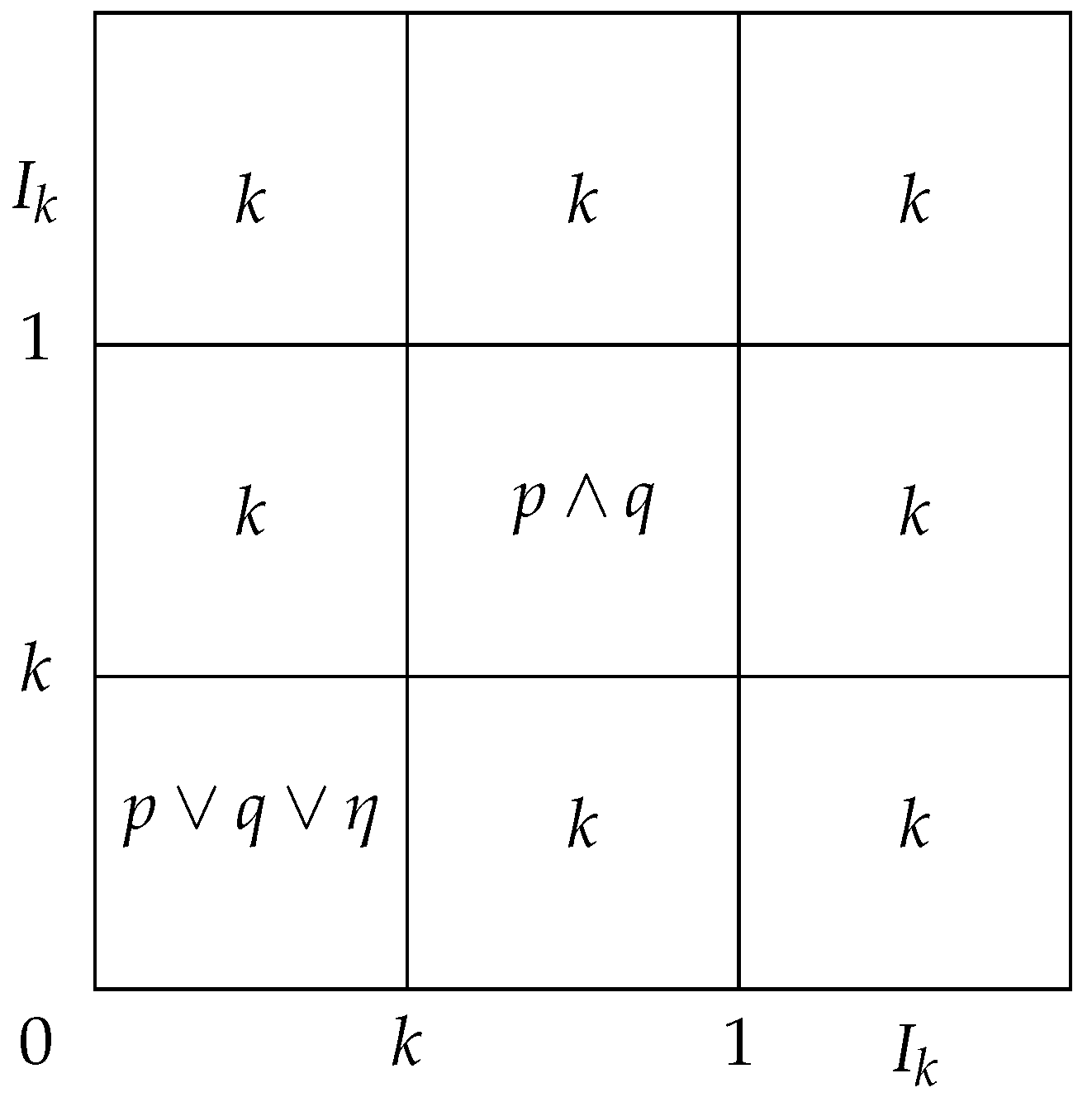
The structure of the nullnorm $Z^{\ast 1}$ given in Formula (2) is summarized in Figure 3.

Remark 1.

In Theorem 1, even if Formula (1) results in a nullnorm on the bounded lattice L, the lattice L may not satisfy $p<q$ for all $p\in [0,k),q\in I_k$. The function $Z_1$ in Theorem 1 is a nullnorm with the annihilator element k on the bounded lattice L. We illustrate this argument by an example as follows. In the following example, it is clear that the lattice $L_2$ does not satisfy the required conditions, even $Z_1$ is a nullnorm on $L_2$.

Example 2.

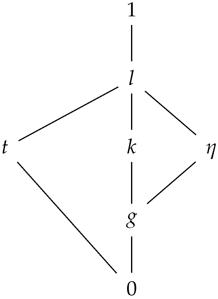
Consider the bounded lattice $(L_2=\{0,g,k,l,t,\eta ,1\},\le )$ characterized by the Hasse diagram in Figure 4. It is clear that $g\in [0,k)$, $t\in I_k$ and $g\nless t$ while the operator Z obtained by Formula (1) and given in

Table 2. The nullnorm Z induced by Formula (1) in Theorem 1.

Z	0	g	k	l	t	$\eta$	1
0	0	g	k	k	g	g	k
g	g	g	k	k	g	g	k
k	k	k	k	k	k	k	k
l	k	k	k	l	k	k	l
t	g	g	k	k	g	g	k
$\eta$	g	g	k	k	g	g	k
1	k	k	k	l	k	k	1

is a nullnorm with the annihilator element k on the bounded lattice $L_2$, when $T=T_{\wedge }$ and $S=S_{\vee }$.

Remark 2.

Observe that Formula (1) given in Theorem 1 may not construct a nullnorm on a bounded lattice L that does not satisfy the condition $p<q$ for all $p\in [0,k)$ and $q\in I_k$ given in Theorem 1; i.e., the condition can not be omitted in general. In the following, in order to show this fact, we give an example of a bounded lattice having some elements $p\in [0,k),q\in I_k$ such that $p\Vert q$, on which the operator $Z_1$ is not a nullnorm.

Example 3.

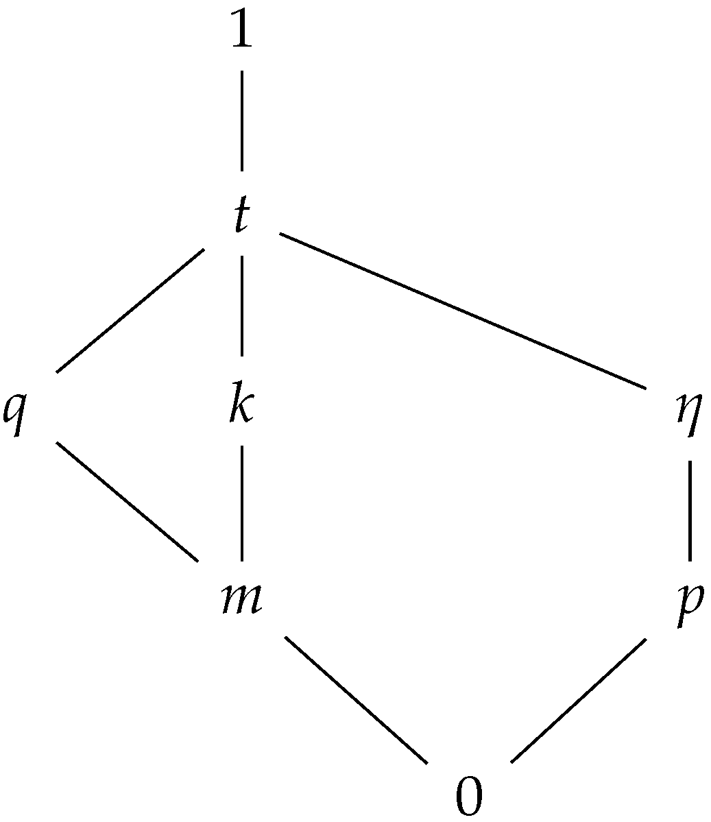
Consider the bounded lattice $(L_3=\{0,k,m,p,q,t,\eta ,1\},\le )$ described in Figure 5.

It is seen that $m\nless \eta$ and $m\nless p$ for the elements $m\in [0,k)$ and $\eta ,p\in I_k$. Considering the Formula (1) in Theorem 1, for the function $Z_1$ on $L_3$, we obtain $Z_1(m,0)=S(m,0)=m\nleqq 0=\eta \wedge k=Z_1(q,0)$ when $m<q$ for the elements $m,q\in L_3$. So, the monotonicity is violated. Therefore, $Z_1$ is not a nullnorm on $L_3$.

In general, the nullnorm $Z_1$ defined in Theorem 1 is different from the nullnorms $V_k^{\left(S\right)}$, $V_k^{\left(T\right)}$, $V_T^{S,R}$, $V_S^{T,F}$, $F_T$, $F_S$, $V_S^T$ and $V_T^S$ in refs. [7,9,14,17]. We illustrate this argument by the following Examples 4 and 5.

Example 4.

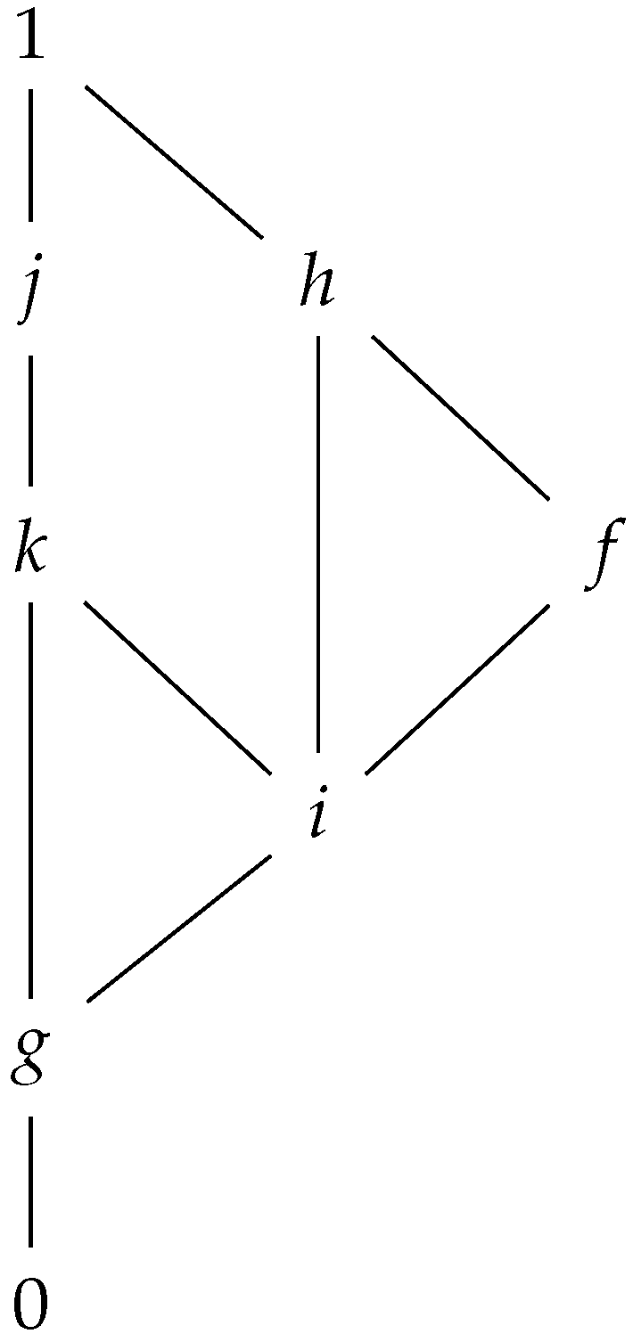
Consider the bounded lattice $(L_4=\{0,f,g,h,i,j,k,1\},\le )$ characterized by the Hasse diagram in Figure 6.

By using the construction methods in refs. [7,9,14,17] and Theorem 1 and put $h=\eta$, $T=T_{\wedge }$ and $S=S_{\vee }$, we have the following:

• $V_k^{\left(S\right)}(j,j)=k\ne j=j\wedge j=Z_1(j,j)$,
• $V_k^{\left(T\right)}(g,i)=k\ne i=g\vee i=Z_1(g,i)$,
• $V_S^{T,F}(h,f)=F(h\vee k,f\vee k)=F(1,1)\ne c=Z_1(h,f)$ (Since $F(1,1)\in [k,1])$,
• $F_T(f,j)=j\ne k=Z_1(f,j)$,
• $V_S^T(g,f)=k\ne i=h\wedge k=Z_1(g,f)$.

Therefore, it is clear that the nullnorm $Z_1$ defined by Formula (1) in Theorem 1 is different from the nullnorms $V_k^{\left(S\right)}$, $V_k^{\left(T\right)}$, $V_S^{T,F}$, $F_T$ and $V_S^T$ given in refs. [7,9,14,17].

Example 5.

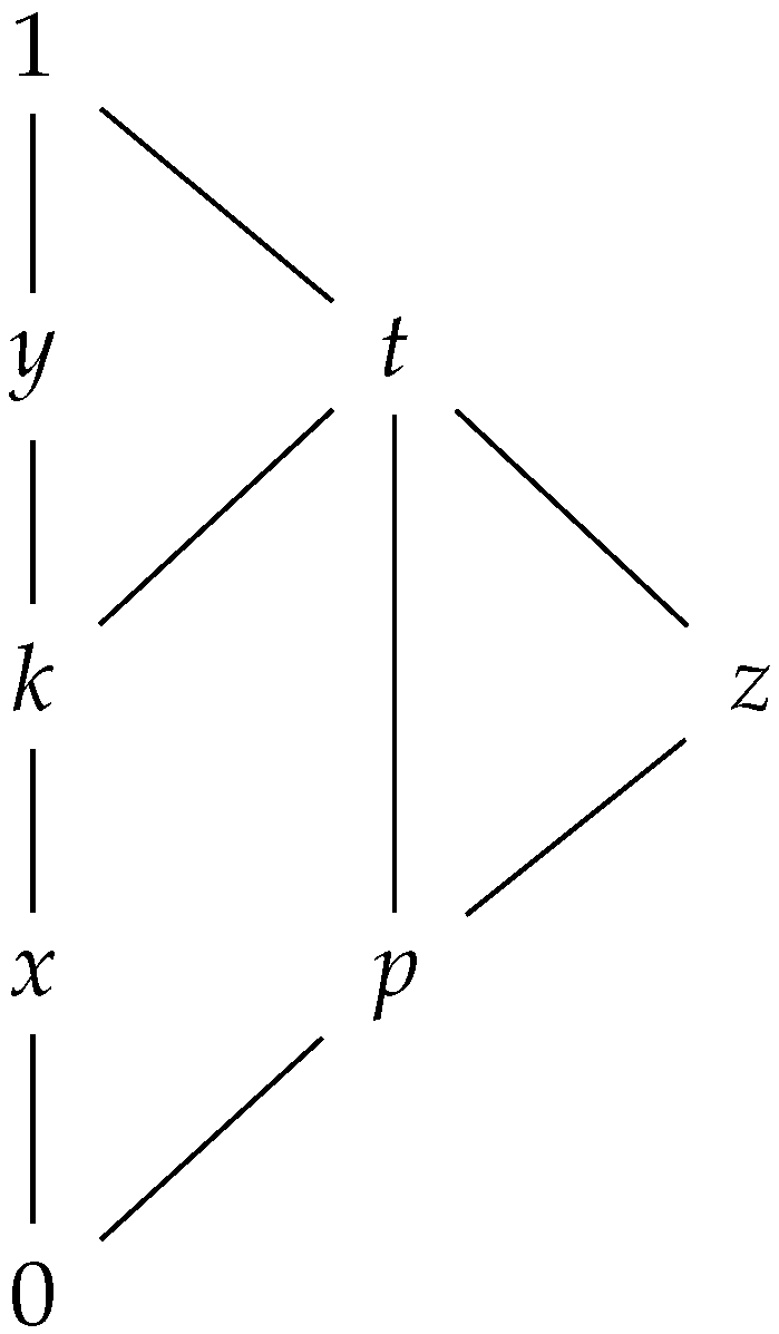
Consider the lattice $(L_5=\{0,k,p,t,x,y,z,1\},\le )$ described in Figure 7.

Let us apply the construction methods in refs. [7,9,14,17] and Theorem 1 and put $z=\eta$, $T=T_{\wedge }$ and $S=S_{\vee }$; then, we have the following:

• $V_T^{S,R}(x,p)=R(x\wedge k,p\wedge k)=R(x,0)\ne 0=z\wedge k=Z_1(x,p)$ (since $R(x,0)\in [x,k]$),
• $F_S(x,p)=x\ne 0=z\wedge k=Z_1(x,p)$,
• $V_T^S(x,p)=S(x\wedge k,p\wedge k)=S(x,0)=x\ne 0=z\wedge k=Z_1(x,p)$ (since $S(x,0)\in [x,k]$).

Thus, it is clearly seen that the nullnorm $Z_1$ defined by Formula (1) in Theorem 1 is different from the nullnorms $V_T^{S,R}$, $F_S$ and $V_T^S$ given in refs. [9,14,17].

Remark 3.

It should be noted that the nullnorm $Z_1$ obtained by Formula (1) and the nullnorm $V_k^{\left(S\right)}$ obtained by Theorem 4 in [7] are the same whenever the t-norm $T=T_D$ on $[k,1]$ in Formula (1) and the t-conorm S on $[0,k]$ in Theorem 4 in [7] satisfies the condition $S(\eta \wedge k,\eta \wedge k)=\eta \wedge k$ and $I_k=\left\{\eta \right\}$. 5Moreover, the nullnorm $Z_1$ obtained by Formula (1) coincides with the nullnorm $V_T^{S,R}$ obtained by Theorem 3.2 in [17] if the t-subconorm R on $[0,k]$ in Theorem 3.2 in [17] satisfies the condition $R(\eta \wedge k,\eta \wedge k)=\eta \wedge k$. In addition, the nullnorm $Z_1$ obtained by Formula (1) coincides with and the nullnorm $V_T^S$ obtained by Theorem 6 in [14] when the t-conorm S on $[0,k]$ in Theorem 6 in [14] satisfies the condition $S(\eta \wedge k,\eta \wedge k)=\eta \wedge k$ and $I_k=\left\{\eta \right\}$.

Based on the element-based construction approach provided by Formula (3) in Theorem 2, which relies on the existence of the element $\eta \in I_k$, we can derive another nullnorm construction method, acquired by considering a t-norm T on the interval $[k,1]$ such that $T(\eta \vee k,\eta \vee k)=\eta \vee k$, and the t-conorm S on the interval $[0,k]$.

Theorem 2.

Let $(L,\le ,0,1)$ be a bounded lattice, $k\in L\setminus \{0,1\}$, $\eta \in I_k$, S be a t-conorm on $[0,k]$ and T be a t-norm on $[k,1]$ satisfying $T(\eta \vee k,\eta \vee k)=\eta \vee k.$ If $p<q$ for all $p\in I_k,q\in (k,1]$, then the function $Z_2:L^2\to L$ defined by

$$Z_2(p,q)=\left\{\begin{array}{cc}S(p,q)\hfill & if(p,q)\in {[0,k)}^2,\hfill \\ T(p,q)\hfill & if(p,q)\in {[k,1]}^2,\hfill \\ \eta \vee k\hfill & if(p,q)\in ((k,1]\cup I_k)\times I_k\cup I_k\times (k,1],\hfill \\ k\hfill & otherwise,\hfill \end{array}\right.$$

(3)

is a nullnorm on L with the annihilator element k.

Proof. 

The proof follows easily from Theorem 1, and therefore it is omitted. □

The structure of the nullnorm $Z_2$ given in Formula (3) is summarized in Figure 8.

Example 6.

Consider the bounded lattice from Example 3, i.e., $(L_3=\{0,k,m,p,q,t,\eta ,1\},\le )$ as shown in Figure 5; then, the nullnorm $Z_2$ on $L_3$ with annihilator element k is obtained as in

Table 3. The nullnorm $Z_2$ induced by Formula (3) in Theorem 2.

$Z_2$	0	k	m	p	q	t	$\eta$	1
0	0	k	m	k	k	k	k	k
k	k	k	k	k	k	k	k	k
m	m	k	k	k	k	k	k	k
p	k	k	k	t	t	t	t	t
q	k	k	k	t	t	t	t	t
t	k	k	k	t	t	t	t	t
$\eta$	k	k	k	t	t	t	t	t
1	k	k	k	t	t	t	t	1

when $T=T_{\wedge }$ and $S=S_W$.

By considering $T=T_{\wedge }$ and $S=S_{\vee }$ in Theorem 2, the following Corollary 2 is obtained.

Corollary 2.

Let $(L,\le ,0,1)$ be a bounded lattice, $k\in L\setminus \{0,1\}$ and $\eta \in I_k$. If $p<q$ for all $p\in I_k,q\in (k,1]$, then the function $Z^2:L^2\to L$ defined by

$$Z^2(p,q)=\left\{\begin{array}{cc}p\vee q\hfill & (p,q)\in {[0,k)}^2,\hfill \\ p\wedge q\hfill & (p,q)\in {[k,1]}^2,\hfill \\ \eta \vee k\hfill & (p,q)\in ((k,1]\cup I_k)\times I_k\cup I_k\times (k,1],\hfill \\ k\hfill & otherwise,\hfill \end{array}\right.$$

(4)

is a nullnorm on L with the annihilator element k.

The structure of the nullnorm $Z^2$ given in Formula (4) is summarized in Figure 9.

Remark 4.

Observe that Formula (3) given in Theorem 2 may construct a nullnorm on a bounded lattice L that does not satisfy the condition $p<q$ for all $p\in I_k,q\in (k,1]$ given in Theorem 2. The function $Z_2$ is a nullnorm on L with the annihilator element k. In order to show this argument, in the following, an example of a bounded lattice not satisfying the mentioned condition is given in which the function $Z_2$ is a nullnorm defined by Formula (3) in Theorem 2.

Example 7.

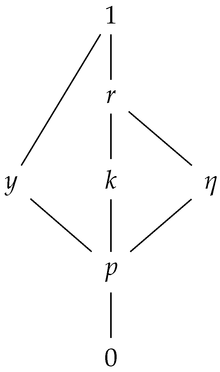
Consider the bounded lattice $(L_6=\{0,k,p,r,y,\eta ,1\},\le )$ characterized by the Hasse diagram in Figure 10.

The lattice $L_6$ does not satisfy the condition of Theorem 2 since $y\in I_k$ and $r\in (k,1]$ such that $y\nless k$. The function Z obtained by Formula (3) in Theorem 2 and given in

Table 4. The nullnorm Z induced by Formula (3) in Theorem 2.

Z	0	k	p	r	y	$\eta$	1
0	0	k	p	k	k	k	k
k	k	k	k	k	k	k	k
p	p	k	k	k	k	k	k
r	k	k	k	r	r	r	r
y	k	k	k	r	r	r	r
$\eta$	k	k	k	r	r	r	r
1	k	k	k	r	r	r	1

, when $T=T_{\wedge }$ and $S=S_W$, is a nullnorm on the bounded lattice $L_6$ with the annihilator element k.

Remark 5.

It should be noted that the nullnorm $Z_2$ obtained by Formula (3) and the nullnorm $V_k^{\left(T\right)}$ obtained by Theorem 4 in [7] are the same whenever the t-conorm $S=S_D$ on $[0,k]$ in Formula (3), the t-norm T on $[k,1]$ in Theorem 4 in [7] satisfies the condition $T(\eta \vee k,\eta \vee k)=\eta \vee k$ and $I_k=\left\{\eta \right\}$. Moreover, the nullnorm $Z_2$ obtained by Formula (3) coincides with the nullnorm $V_S^{T,F}$$\left(V_S^T\right)$ obtained by Theorem 3.3 (Theorem 6) in [17] ([14]), and the t-subnorm F (t- norm T) on $[k,1]$ in Theorem 3.3 (Theorem 6) in [17] ([14]) satisfies the condition $F(\eta \vee k,\eta \vee k)=\eta \vee k$$\left(T\right(\eta \vee k,\eta \vee k)=\eta \vee k)$ and $I_k=\left\{\eta \right\}$.

Now, in the following, we introduce a construction method for nullnorms with the annihilator element k based on the element $\eta \in (0,k)$. Our construction method exploits the existence of a t-norm T on the subinterval $[0,k]$. It should be pointed out that our construction method does not need any constraints here.

Theorem 3.

Let $(L,\le ,0,1)$ be a bounded lattice, $k\in L\setminus \{0,1\}$, $\eta \in (0,k)$ and T be a t-norm on $[k,1]$. Then, the function $Z_3:L^2\to L$ defined by

$$Z_3(p,q)=\left\{\begin{array}{cc}p\vee q\vee \eta \hfill & if(p,q)\in {(0,k)}^2,\hfill \\ T(p,q)\hfill & if(p,q)\in {[k,1]}^2,\hfill \\ p\vee q\hfill & if(p,q)\in \left\{0\right\}\times [0,k)\cup [0,k)\times \left\{0\right\},\hfill \\ k\hfill & otherwise,\hfill \end{array}\right.$$

(5)

is a nullnorm on L with the annihilator element k.

Proof. 

By the definition of the function $Z_3$, it is clear that $Z_3$ is a commutative function with the annihilator element k. Now, in the following, let us check that the monotonicity and associativity hold.

(i)

Monotonicity: Let us show that for all elements $p,q\in L$ with $p\le q$, $Z_3(p,r)\le Z_3(q,r)$ for all $r\in L$. If p and q are both elements of $\left\{0\right\}$ or $(0,k)$ or $\left\{k\right\}$ or $(k,1)$ or $I_k$, $Z_3(p,r)\le Z_3(q,r)$ is always satisfied for all $r\in L$ since $p\le q$. If $p=1$ or $r\in I_k$, the inequality is satisfied; therefore, they are omitted. The proof then considers all of the remaining cases.

1.

Let $p=0$.

(1.1)

$q\in (0,k)$,

(1.1.1)

If $r=0$, then $Z_3(p,r)=p\vee r\le q\vee r=Z_3(q,r).$

(1.1.2)

If $r\in (0,k)$, then $Z_3(p,r)=p\vee r\le q\vee r\vee \eta =Z_3(q,r).$

(1.1.3)

If $r\in [k,1)$, then $Z_3(p,r)=k=Z_3(q,r).$

(1.2)

$q\in \left\{k\right\}\cup I_k$,

(1.2.1)

If $r\in [0,k)$, then $Z_3(p,r)=p\vee r\le k=Z_3(q,r).$

(1.2.2)

If $r\in [k,1)$, then $Z_3(p,r)=k=Z_3(q,r).$

(1.3)

$q\in (k,1)$,

(1.3.1)

If $r\in [0,k)$, then $Z_3(p,r)=p\vee r\le k=Z_3(q,r).$

(1.3.2)

If $r\in [k,1)$, then $Z_3(p,r)=k\le T(q,r)=Z_3(q,r).$

2.

Let $p\in (0,k)$.

(2.1)

$q\in \left\{k\right\}\cup I_k$,

(2.1.1)

If $r=0$, then $Z_3(p,r)=p\vee r\le k=Z_3(q,r).$

(2.1.2)

If $r\in (0,k)$, then $Z_3(p,r)=p\vee r\vee \eta \le k=Z_3(q,r).$

(2.1.3)

If $r\in [k,1)$, then $Z_3(p,r)=k=Z_3(q,r).$

(2.2)

$q\in (k,1)$,

(2.2.1)

If $r=0$, then $Z_3(p,r)=p\vee r\le k=Z_3(q,r).$

(2.2.2)

If $r\in (0,k)$, then $Z_3(p,r)=p\vee r\vee \eta \le k=Z_3(q,r).$

(2.2.3)

If $r\in [k,1)$, then $Z_3(p,r)=k\le T(q,r)=Z_3(q,r).$

3.

Let $p=k$,

(3.1)

$q\in (k,1)$,

(3.1.1)

If $r\in [0,k]$, then $Z_3(p,r)=k=Z_3(q,r).$

(3.1.2)

If $r\in [k,1)$, then $Z_3(p,r)=k\le T(q,r)=Z_3(q,r).$

4.

Let $p\in I_k$,

(4.1)

$q\in (k,1)$,

(4.1.1)

If $r\in [0,k)$, then $Z_3(p,r)=k=Z_3(q,r).$

(4.1.2)

If $r\in [k,1)$, then $Z_3(p,r)=k\le T(q,r)=Z_3(q,r).$

(ii)

Associativity: We demonstrate that $Z_3(p,Z_3(q,r))=Z_3(Z_3(p,q),r)$ for all $p,q,r\in L$. If at least one of the elements $p,q,r$ belongs to the set $I_k\cup \left\{k\right\}$, the equality is satisfied; therefore, they are omitted. Again, taking that $Z_3$ is commutative into account, the proof considers all of the remaining cases.

1.

Let $p=0$.

(1.1)

$q=0$,

(1.1.1)

If $r\in [0,k)$, then $Z_3(p,Z_3(q,r))=Z_3(p,q\vee r)=p\vee q\vee r=Z_3(p\vee q,r)=Z_3(Z_3(p,q),r).$

(1.1.2)

If $r\in (k,1]$, then $Z_3(p,Z_3(q,r))=Z_3(p,k)=k=Z_3(p\vee q,r)=Z_3(Z_3(p,q),r).$

(1.2)

$q\in (0,k)$,

(1.2.1)

If $r=0$, then $Z_3(p,Z_3(q,r))=Z_3(p,q\vee r)=p\vee q\vee r=Z_3(p\vee q,r)=Z_3(Z_3(p,q),r).$

(1.2.2)

If $r\in (0,k)$, then $Z_3(p,Z_3(q,r))=Z_3(p,q\vee r\vee \eta )=p\vee q\vee r\vee \eta =Z_3(p\vee q,r)=Z_3(Z_3(p,q),r).$

(1.2.3)

If $r\in (k,1]$, then $Z_3(p,Z_3(q,r))=Z_3(p,k)=k=Z_3(p\vee q,r)=Z_3(Z_3(p,q),r).$

(1.3)

$q\in (k,1]$,

(1.3.1)

If $r\in [0,k)$, then $Z_3(p,Z_3(q,r))=Z_3(p,k)=k=Z_3(k,r)=Z_3(Z_3(p,q),r).$

(1.3.2)

If $r\in (k,1]$, then $Z_3(p,Z_3(q,r))=Z_3(p,T(q,r))=k=Z_3(k,r)=Z_3(Z_3(p,q),r).$

2.

Let $p\in (0,k)$.

(2.1)

$q=0$,

(2.1.1)

If $r\in (0,k)$, then $Z_3(p,Z_3(q,r))=Z_3(p,q\vee r)=p\vee q\vee r\vee \eta =Z_3(p\vee q,r)=Z_3(Z_3(p,q),r).$

(2.1.2)

If $r\in (k,1]$, then $Z_3(p,Z_3(q,r))=Z_3(p,k)=k=Z_3(p\vee q,r)=Z_3(Z_3(p,q),r).$

(2.2)

$q\in (0,k)$,

(2.2.1)

If $r\in (0,k)$, then $Z_3(p,Z_3(q,r))=Z_3(p,q\vee r\vee \eta )=p\vee q\vee r\vee \eta =Z_3(p\vee q\vee \eta ,r)=Z_3(Z_3(p,q),r).$

(2.2.2)

If $r\in (k,1]$, then $Z_3(p,Z_3(q,r))=Z_3(p,k)=k=Z_3(p\vee q\vee \eta ,r)=Z_3(Z_3(p,q),r).$

(2.3)

$q\in (k,1]$,

(2.3.1)

If $r\in (0,k)$, then $Z_3(p,Z_3(q,r))=Z_3(p,k)=k=Z_3(k,r)=Z_3(Z_3(p,q),r).$

(2.3.2)

If $r\in (k,1]$, then $Z_3(p,Z_3(q,r))=Z_3(p,T(q,r))=k=Z_3(k,r)=Z_3(Z_3(p,q),r).$

3.

Let $p\in (k,1]$.

(3.1)

$q=0$,

(3.1.1)

If $r\in (0,k)$, then $Z_3(p,Z_3(q,r))=Z_3(p,q\vee r)=k=Z_3(k,r)=Z_3(Z_3(p,q),r).$

(3.2)

$q\in (0,k)$,

(3.2.1)

If $r\in (k,1]$, then $Z_3(p,Z_3(q,r))=Z_3(p,k)=k=Z_3(k,r)=Z_3(Z_3(p,q),r).$

(3.3)

$q\in (k,1]$,

(3.3.1)

If $r\in (k,1]$, then $Z_3(p,Z_3(q,r))=Z_3(p,T(q,r))=T(p,T(q,r))=T(T(p,q),r)=Z_3(T(p,q),r)=Z_3(Z_3(p,q),r).$

We conclude that $Z_3$ is a nullnorm on L with the annihilator element k. □

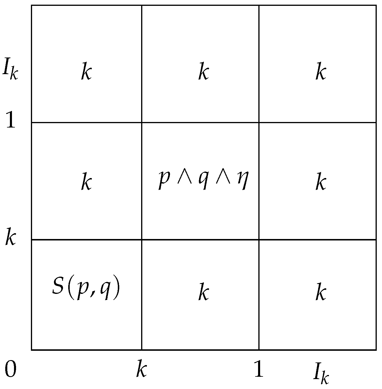
The structure of the nullnorm $Z_3$ given in Formula (5) is summarized in Figure 11.

Remark 6.

(i) If we take $S(p,q)=\left\{\begin{array}{cc}p\vee q\hfill & 0\in \{p,q\}\hfill \\ p\vee q\vee \eta \hfill & otherwise\hfill \end{array}\right.$ and $R(p\wedge k,q\wedge k)=k$ in ref. [17], the nullnorm $V_T^{S,R}$ coincides with the nullnorm $Z_3$ obtained by Formula (5).

• (ii) If we take $S(p,q)=\left\{\begin{array}{cc}p\vee q\hfill & 0\in \{p,q\}\hfill \\ p\vee q\vee \eta \hfill & otherwise\hfill \end{array}\right.$ and $F(p\vee k,q\vee k)=k$ in Formula [17], the nullnorm $V_s^{T,F}$ coincides with the nullnorm $Z_3$ obtained by Formula (5).

Now, we give the following examples in order to show that the nullnorm $Z_3$ defined by Formula (5) in Theorem 3 is different from those nullnorms obtained by the construction methods in the literature in general.

Example 8.

Consider the bounded lattice from Example 4, i.e., $(L_4=\{0,f,g,h,i,j,k,1\},\le )$ characterized by the Hasse diagram in Figure 6.

By using the construction methods in [7,9,14] and Theorem 3 and putting $g=\eta$, $T=T_{\wedge }$ as taken, we obtain the following:

• $V_k^{\left(S\right)}(j,j)=k\ne j=j\wedge j=T(j,j)=Z_3(j,j)$,
• $V_k^{\left(T\right)}(g,g)=k\ne g=g\vee g\vee g=Z_3(g,g)$,
• $F_T(j,f)=j\ne k=Z_3(f,j)$,
• $V_S^T(h,h)=T(h\vee k,h\vee k)=T(1,1)=1\ne k=Z_3(h,h)$.

Therefore, it is clear that the nullnorm $Z_3$ defined by Formula (5) in Theorem 3 is different from the nullnorms $V_k^{\left(S\right)}$, $V_k^{\left(T\right)}$, $F_T$ and $V_S^T$ given in refs. [7,9,14].

Example 9.

Consider the bounded lattice from Example 5, i.e., $(L_5=\{0,k,p,t,x,y,z,1\},\le ,0,1)$ characterized by the Hasse diagram in Figure 7.

Let us apply the construction methods in refs. [9,14] and Theorem 3, and putting $x=\eta$, $S=S_{\vee }$ as taken, we obtain the following:

• $F_S(x,p)=x\ne k=Z_3(x,p)$,
• $V_T^S(p,z)=S(p\wedge k,z\wedge k)=S(0,0)=0\ne k=Z_3(p,z)$.

Thus, it is clearly seen that the nullnorm $Z_3$ defined by Formula (5) in Theorem 3 is different from the nullnorms $F_S$ and $V_T^S$ given in refs. [9,14].

In the following Corollary 3, by taking $T=T_{\wedge }$ for the nullnorm $Z_3$ in Theorem 3, we obtain the following nullnorm $Z^3$ on L having an annihilator element k without any constraints.

Corollary 3.

Let $(L,\le ,0,1)$ be a bounded lattice, $k\in L\setminus \{0,1\}$ and $\eta \in (0,k)$. Then, the function $Z^3:L^2\to L$ defined by

$$Z^3(p,q)=\left\{\begin{array}{cc}p\vee q\vee \eta \hfill & if(p,q)\in {(0,k)}^2,\hfill \\ p\wedge q\hfill & if(p,q)\in {[k,1]}^2,\hfill \\ p\vee q\hfill & if(p,q)\in \left\{0\right\}\times [0,k)\cup [0,k)\times \left\{0\right\},\hfill \\ k\hfill & otherwise,\hfill \end{array}\right.$$

(6)

is a nullnorm on L with the annihilator element k.

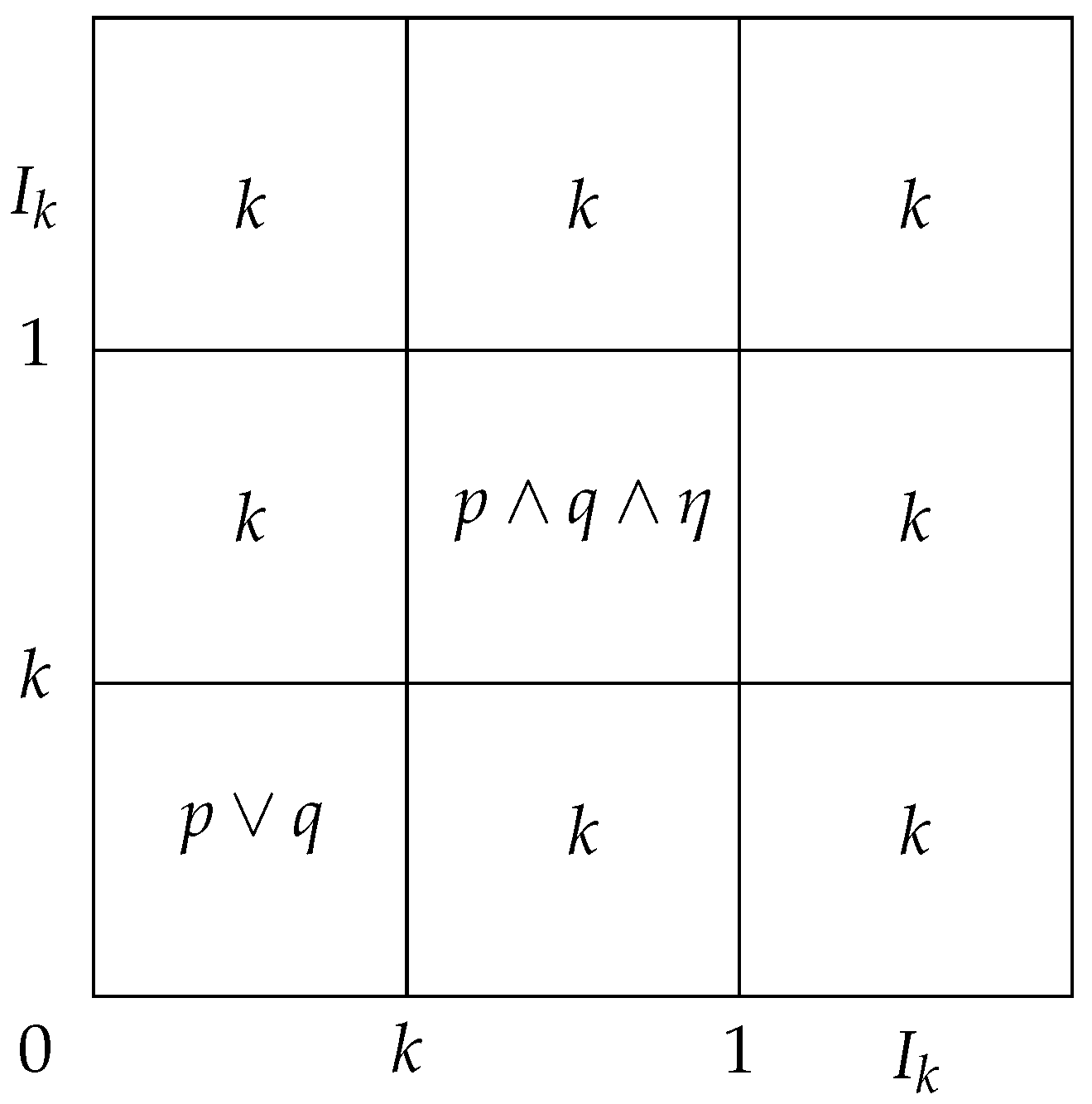
The structure of the nullnorm $Z^3$ given in Formula (6) is summarized in Figure 12.

Next, we present a construction method for nullnorms induced by the element $\eta \in (k,1)$, which utilizes the existence of a t-conorm on $[0,k]$.

Theorem 4.

Let $(L,\le ,0,1)$ be a bounded lattice, $k\in L\setminus \{0,1\}$, $\eta \in (k,1)$ and S be a t-conorm on $[0,k]$. Then, the function $Z_4:L^2\to L$ defined by

$$Z_4(p,q)=\left\{\begin{array}{cc}S(p,q)\hfill & if(p,q)\in {[0,k)}^2,\hfill \\ p\wedge q\wedge \eta \hfill & if(p,q)\in {[k,1)}^2,\hfill \\ p\wedge q\hfill & if(p,q)\in \left\{1\right\}\times [k,1]\cup [k,1]\times \left\{1\right\},\hfill \\ k\hfill & otherwise,\hfill \end{array}\right.$$

(7)

is a nullnorm on L with the annihilator element k.

Proof. 

The proof follows easily from Theorem 3, and therefore it is omitted. □

The structure of the nullnorm $Z_4$ given in Formula (7) is summarized in Figure 13.

In order to show that the nullnorm $Z_4$ defined by Formula (7) in Theorem 4 is different from the nullnorms obtained by the construction methods in the literature, we present the following examples.

Remark 7.

(i) If we take $T(p,q)=\left\{\begin{array}{cc}p\wedge q\hfill & 1\in \{p,q\}\hfill \\ p\wedge q\wedge \eta \hfill & otherwise\hfill \end{array}\right.$ and $R(p\wedge k,q\wedge k)=k$ in [17], the nullnorm $V_T^{S,R}$ coincides with the nullnorm $Z_4$ obtained by Formula (7).

• (ii) If we take $T(p,q)=\left\{\begin{array}{cc}p\wedge q\hfill & 1\in \{p,q\}\hfill \\ p\wedge q\wedge \eta \hfill & otherwise\hfill \end{array}\right.$ and $F(p\vee k,q\vee k)=k$ in ref. [17], the nullnorm $V_s^{T,F}$ coincides with the nullnorm $Z_4$ obtained by Formula (7).

Example 10.

Consider the bounded lattice from Example 4, i.e., $(L_4=\{0,f,g,h,i,j,k,1\},\le )$ characterized by the Hasse diagram in Figure 6.

By taking the construction methods in [7,9,14] into account alongside Theorem 4 and putting $j=\eta$, $T=T_{\wedge }$ as taken, we obtain the following:

• $V_k^{\left(S\right)}(j,j)=k\ne j=j\wedge j\wedge j=Z_4(j,j)$,
• $V_k^{\left(T\right)}(h,h)=T(h\vee k,h\vee k)=T(1,1)=1\ne k=Z_4(h,h)$,
• $F_T(i,f)=i\vee (f\wedge k)=i\vee i=i\ne k=Z_4(i,f)$,
• $V_S^T(f,f)=T(f\vee k,f\vee k)=T(1,1)=1\ne k=Z_4(f,f)$.

Therefore, it is clear that the nullnorm $Z_4$ defined by Formula (7) in Theorem 4 is different from the nullnorms $V_k^{\left(S\right)}$, $V_k^{\left(T\right)}$, $F_T$ and $V_S^T$ given in refs. [7,9,14].

Example 11.

Consider the bounded lattice from Example 5, i.e., $(L_5=\{0,k,p,t,x,y,z,1\},\le )$ characterized by the Hasse diagram in Figure 7.

Let us apply the construction methods in [9,14] and Theorem 4, and putting $y=\eta$, $S=S_{\vee }$ as taken, we obtain the following:

• $F_S(x,z)=x\ne k=Z_4(x,z)$,
• $V_T^S(z,z)=S(z\wedge k,z\wedge k)=S(0,0)=0\ne k=Z_4(z,z)$.

Thus, it is clearly seen that the nullnorm $Z_4$ defined by Formula (7) in Theorem 4 is different from the nullnorms $F_S$ and $V_T^S$ given in refs. [9,14].

In Theorem 4, putting the t-conorm $S=S_{\vee }$, we obtain the following element-based construction method for nullnorms via the element $\eta \in (k,1)$ of a lattice.

Corollary 4.

Let $(L,\le ,0,1)$ be a bounded lattice, $k\in L\setminus \{0,1\}$, $\eta \in (k,1)$. Then, the function $Z^4:L^2\to L$ defined by

$$Z^4(p,q)=\left\{\begin{array}{cc}p\vee q\hfill & if(p,q)\in {[0,k)}^2,\hfill \\ p\wedge q\wedge \eta \hfill & if(p,q)\in {[k,1)}^2,\hfill \\ p\wedge q\hfill & if(p,q)\in \left\{1\right\}\times (k,1]\cup (k,1]\times \left\{1\right\},\hfill \\ k\hfill & otherwise,\hfill \end{array}\right.$$

(8)

is a nullnorm on L with the annihilator element k.

The structure of the nullnorm $Z^4$ given in Formula (8) is summarized in Figure 14.

4. Conclusions

Nullnorms on bounded lattices, particularly their representations and constructions, have been the subject of intensive study in recent years. Representation issues were deeply studied, e.g., in [16], considering elements comparable with the given annihilator. We have introduced new construction methods for such situations in Theorems 1, 3 and 4. Representations dealing with elements incomparable with the considered annihilator were studied, e.g., in [21]. The authors there have observed that the difficulty in constructing nullnorms on bounded lattices lies just in the cases where there are elements incomparable with the considered annihilator k. This problem was discussed in our Corollaries 1 and 2, which can be seen as most important results of this paper. Observe that numerous examples transparently illustrate the obtained results, stressing the difference between our approaches and those in the existing literature. We believe that the presented methods may inspire the development of new construction techniques for other types of aggregation functions.

References

1. Calvo, T.; De Baets, B.; Fodor, J. The functional equations of Frank and Alsina for uninorms and nullnorm. Fuzzy Sets Syst. 2001, 120, 385–394. [Google Scholar] [CrossRef]
2. Mas, M.; Mayor, G.; Torrens, J. t-operators. Int. J. Uncertain. Fuzziness Knowl. Based Syst. 1999, 7, 31–50. [Google Scholar] [CrossRef]
3. Mas, M.; Mayor, G.; Torrens, J. The distributivity condition for uninorms and t-operators. Fuzzy Sets Syst. 2002, 128, 209–225. [Google Scholar] [CrossRef]
4. Drygaś, P. A characterization of idempotent nullnorms. Fuzzy Sets Syst. 2004, 145, 455–461. [Google Scholar] [CrossRef]
5. Qin, F.; Zhao, B. The distributive equations for idempotent uninorms and nullnorms. Fuzzy Sets Syst. 2005, 155, 446–458. [Google Scholar] [CrossRef]
6. Xie, A.; Liu, H. On the distributivity of uninorms over nullnorms. Fuzzy Sets Syst. 2013, 211, 62–72. [Google Scholar] [CrossRef]
7. Karaçal, F.; İnce, M.A.; Mesiar, R. Nullnorms on bounded lattices. Inf. Sci. 2015, 325, 227–236. [Google Scholar] [CrossRef]
8. Çaylı, G.D.; Karaçal, F. Some remarks on idempotent nullnorms on bounded lattices. In Aggregation Functions in Theory and in Practice; Springer International Publishing: Berlin/Heidelberg, Germany, 2018; pp. 31–39. [Google Scholar]
9. Çaylı, G.D. Nullnorms on bounded lattices derived from t-norms and t-conorms. Inf. Sci. 2020, 512, 1134–1154. [Google Scholar] [CrossRef]
10. Çaylı, G.D. Construction methods for idempotent nullnorms on bounded lattices. Appl. Math. Comput. 2020, 366, 124746. [Google Scholar] [CrossRef]
11. Çaylı, G.D. Some results about nullnorms on bounded lattices. Fuzzy Sets Syst. 2020, 386, 105–131. [Google Scholar] [CrossRef]
12. Çaylı, G.D. Construction of nullnorms on some special classes of bounded lattices. Int. J. Approx. Reason. 2021, 134, 111–128. [Google Scholar] [CrossRef]
13. Dan, Y.; Hu, B.Q.; De Baets, B. Nullnorms on bounded lattices constructed by means of closure and interior operators. Fuzzy Sets Syst. 2022, 439, 142–156. [Google Scholar] [CrossRef]
14. Ertuğrul, Ü. Construction of nullnorms on bounded lattices and an equivalence relation on nullnorms. Fuzzy Sets Syst. 2018, 334, 94–109. [Google Scholar] [CrossRef]
15. İnce, M.A.; Karaçal, F.; Mesiar, R. Medians and nullnorms on bounded lattices. Fuzzy Sets Syst. 2016, 289, 74–81. [Google Scholar] [CrossRef]
16. Sun, X.; Liu, H. Representation of nullnorms on bounded lattices. Inf. Sci. 2020, 539, 269–276. [Google Scholar] [CrossRef]
17. Xie, J.; Ji, W. New constructions of nullnorms on bounded lattices. J. Appl. Math. Phys. 2021, 9, 1–10. [Google Scholar] [CrossRef]
18. Birkhoff, G. Lattice Theory; American Mathematical Society Colloquium Publishers: Providence, RI, USA, 1967. [Google Scholar]
19. Klement, E.P.; Mesiar, R.; Pap, E. Triangular Norms; Kluwer Academic Publishers: Dordrecht, The Netherlands, 2000. [Google Scholar]
20. Karaçal, F.; Şanlı, Z. Some new construction methods of t-norms and t-conorms on bounded lattices. Fuzzy Sets Syst. 2022, 451, 84–93. [Google Scholar] [CrossRef]
21. Zhang, H.P.; Ouyang, Y.; Wang, Z.; De Baets, B. A complete representation theorem for nullnorms on bounded lattices with ample illustrations. Fuzzy Sets Syst. 2022, 439, 157–169. [Google Scholar] [CrossRef]
Figure 1. The structure of the nullnorm Z 1 .
Axioms 14 00856 g001
Figure 2. Hasse diagram of L 1 .
Axioms 14 00856 g002
Figure 3. The structure of the nullnorm Z 1 .
Axioms 14 00856 g003
Figure 4. Hasse diagram of L 2 .
Axioms 14 00856 g004
Figure 5. Hasse diagram of L 3 .
Axioms 14 00856 g005
Figure 6. Hasse diagram of L 4 .
Axioms 14 00856 g006
Figure 7. Hasse diagram of L 5 .
Axioms 14 00856 g007
Figure 8. The structure of the nullnorm Z 2 .
Axioms 14 00856 g008
Figure 9. The structure of the nullnorm Z 2 .
Axioms 14 00856 g009
Figure 10. Hasse diagram of L 6 .
Axioms 14 00856 g010
Figure 11. The structure of the nullnorm Z 3 .
Axioms 14 00856 g011
Figure 12. The structure of the nullnorm Z 3 .
Axioms 14 00856 g012
Figure 13. The structure of the nullnorm Z 4 .
Axioms 14 00856 g013
Figure 14. The structure of the nullnorm Z 4 .
Axioms 14 00856 g014