Article

Solving the Fornberg–Whitham Model Derived from Gilson–Pickering Equations by Analytical Methods

by
Donal O’Regan
1,
Safoura Rezaei Aderyani
2,
Reza Saadati
2,* and
Tofigh Allahviranloo
3
1
School of Mathematical and Statistical Sciences, University of Galway, University Road, H91 TK33 Galway, Ireland
2
School of Mathematics, Iran University of Science and Technology, Narmak, Tehran 13114-16846, Iran
3
Research Center of Performance and Productivity Analysis, Istinye University, 34010 Istanbul, Turkey
*
Author to whom correspondence should be addressed.
Axioms 2024, 13(2), 74; https://doi.org/10.3390/axioms13020074
Submission received: 17 November 2023 / Revised: 3 January 2024 / Accepted: 17 January 2024 / Published: 23 January 2024

Abstract

:
This paper focuses on obtaining traveling wave solutions of the Fornberg–Whitham model derived from Gilson–Pickering equations, which describe the prorogation of waves in crystal lattice theory and plasma physics by some analytical techniques, i.e., the exp-function method (EFM), the multi-exp function method (MEFM) and the multi hyperbolic tangent method (MHTM). We analyze and compare them to show that MEFM is the optimum method.

1. Introduction

Nonlinear partial differential equations (NPDEs) are a significant tool for the analysis of nonlinear physical processes and natural phenomena. Indeed, NPDEs play a major role in the description of the physical behavior of real-world processes and dynamical phenomena such as in ocean engineering, physics, fluid mechanics, geochemistry, plasma physics, optical fibers, geophysics, and many other scientific areas. Researchers have focused on finding the analytical or exact solutions to problems which contributes to the analysis of the actual system characteristics. A number of years ago, different efficient and significant methods were developed to obtain solutions, including: the trial equation method, the modified trial equation method [1], the direct algebraic method, the Sine-Gordon expansion method [2], the first integral method, the functional variable method [3], the rational ( G / G 2 ) -expansion method [4,5], the Nucci’s reduction method, the extended hyperbolic method [6], the generalized invariant subspace method [7], the new Kudryashov approach [8], and many others [9,10,11,12,13,14,15].
The EFM [16] proposed by Ji-Huan He and Xu-Hong Wu in 2006 provides us with a straightforward and effective method for obtaining generalized solitary wave solutions and periodic solutions of NLEEs. The method has been applied to many kinds of equations like the double sine-Gordon equation [17], Burger equations [18], Maccari’s system [19], the Klein-Gordon equation [20], the combined KdV-mKdV equation [21], variant Boussinesq equations [22], the Broer–Kaup–Kupershmidt equations [23], variable-coefficient equations [24], high-dimensional equations, discrete equations and so on [25,26,27]. In 2009, Dai et al. [28] generalized the EFM to solve stochastic equations. In 2010, Zhang [29] improved the EFM to obtain not only generalized solitary wave solutions and periodic solutions but also rational solutions. These studies show that the EFM is straightforward, concise, and its applications are promising. The EFM is only concerned about the traveling wave solutions of NPDEs. It is clear that there are multiple wave solutions to NPDEs, for instance, multiple solutions to several significant models like Hirota’s difference equation and the Kdv equation. Thus, there should be a similar technique for obtaining multiple wave solutions to NPDEs. In [30], the authors presented the MEFM, to compute the multiple solutions to the (3+1)-dimensional potential-Yu-Toda-Sasa-Fukuyama equation. The mentioned method is motivated because it is easy to use and also because of the capability of computer algebra systems and the method provides a direct and systematic solution procedure that generalizes Hirota’s perturbation method [31].
In this work, we analytically study the traveling wave solutions of the following Gilson–Pickering equation (GPE) as a nonlinear third-order PDE as
u t A u x x t + 2 B u x u u x x x C u u x D u x u x x = 0 , ( x , t ) ( a , b ) × ( 0 , T ] ,
where u is an unknown function that should be determined, and the subscripts denote the partial derivative, the parameters, A , B , and C are nonzero real numbers, and T is a final time.
Gilson and Pickering [32] first introduced the GPE in 1995. There are three types of special cases for the nonlinear GPE based on specific choices of its parameters. When A = 1 , C = 1 , D = 3 , and B = 0.5 , the GPE converts to the Fornberg–Whitham model, which was developed to analyze the qualitative characteristics of wave breakage and admits a wave of the highest height [32]. For A = 1 , C = 3 and D = 2 , the GPE corresponds to the Fuchssteiner-Fokas-Camassa-Holm model, which is a completely integrable NPDE that arises at various levels of approximation in shallow water theory in [33], and when A = 0 , C = 1 , D = 3 , and B = 0 , the GPE becomes the Rosenau-Hyman model, which occurs in the study of the influence of nonlinear dispersion on the structure of patterns in liquid drops [34]. The Camassa-Holm equation (CHE) constitutes the main form of the GPE [33]. The CHE is an NPDE capable of modeling waves in shallow water [33]. This PDE was introduced by Camassa and Holm [33] and has been demonstrated to have a robust mathematical structure. A significant property of this PDE is its acceptance of non-smooth and smooth solitary wave solutions that are solitons. One can enforce non-smooth or smooth solutions by twisting a parameter in the CHE. Peakons is the name given to the non-smooth solutions, which are solitons that have sharp cusps (or peaks). This leads to a discontinuous derivative of the soliton. Hence, these peakons are solutions merely in the distributional or weak sense. Interested readers can find further analyses regarding the physical and mathematical background of the CHE in the work [33]. Some analytical and numerical methods are also available for finding the solutions of the GPE. Irshad and Tauseef [35] employed the tanh-coth method for the numerical solution of GPE. Fan et al. [36] applied the G / G -expansion scheme for solving the GPE. Chen et al. [37] adopted the qualitative theory of polynomial differential system to study travelling wave solutions of the GPE, whereas Khakzad and Garshasbi [38] combined a meshfree technique with the Crank–Nicolson scheme to simulate the CHE. Saffarian and Zabihi [39] used a not-a-knot meshfree technique to approximate the GPE, while Ali and Mehanna [40] implemented the finite difference (FD) method to solve the GPE. Bilal et al. [41] developed the G / G 2 -expansion and expansion function methods to derive new exact wave structures of the GPE. Kamal Ali et al. [42] considered the 1 / G -expansion and generalized exponential rational function approaches based on a homogeneous balance technique to construct solitary wave solutions of the GPE. Yokuş et al. [43] constructed the soliton solutions of the GPE with the help of the sinh-Gordon function. Rezazadeh et al. [44] considered the exponential rational function and the Jacobi elliptic functions schemes to find new wave surfaces of the GPE. Samir et al. [45] implemented a modified extended mapping technique to obtain solitary wave solutions of the GPE.
The GP problem explains wave propagation in plasma physics and crystal lattice theory. From the surface of the Sun to the heliopause, plasma fills the distance between the planets. Without a doubt, plasma exists in low quantities around distant stars and across much interstellar or intergalactic space. There are astrophysical plasmas in the accretion disks that surround stars and compact objects like white dwarfs, neutron stars, and black holes in binary star systems. Since plasmas may exist in a wide variety of temperatures and densities, they have many applications in the academic and industrial worlds. Plasma spraying, etching in microelectronics, metal cutting, and welding are commonplace in industrial and extractive metallurgy; fuel ignition and exhaust cleaning are used frequently in cars; supersonic combustion engines are used in aerospace engineering [46,47,48].
In this paper, the authors develope several soliton wave solutions for the GP problem. These sorts of solutions are required for the theory of crystal lattices and for studying wave motion in plasma. On the researched model, several analytical techniques including the exp function method, the multi-exp function method and the multi-hyperbolic tangent method [49,50] will be effectively applied which formulate a solution algorithm for calculating multiple wave solutions to the GP model containing one-soliton, two-soliton and three-soliton-type solutions.

2. Analysis of the MEFM, the EFM and the MHTM

2.1. The Procedure of EFM

Here, we propose the basic idea of the EFM as follows [49,50]:
  • Step 1: Consider the general nonlinear partial differential equation of the type:
N ( u , u x , u t , u t t , u x x , u x x x , ) = 0 .
  • Step 2: Let:
Ξ = α x + β t , u = U ( Ξ ) ,
where β and α are fixed.
  • Step 3: Rewrite (1) as
N ˜ ( U , U , U , U , ) = 0 ,
where the prime denotes the derivative with respect to Ξ .
  • Step 4: Consider the wave solutions as:
U ( Ξ ) = n = c d a n e n Ξ m = p q b m e m Ξ = a c e c Ξ + + a d e d Ξ b p e p Ξ + + b q e q Ξ ,
in which q ,   d ,  c and p are positive integers and also a n and b n are constants that are not known and to be determined later.
  • Step 5: To choose the value of p and c, (and similarly d and q), we should balance the linear term of highest (lowest) order of Equation (4) with the highest (lowest) order nonlinear term.

2.2. The Procedure of the MEFM

In this Subsection, we formulate the MEFM [49,50] by considering
N ( x , t , u t , u x , u t t , u x x , ) = 0 ,
where u = u ( x , t ) .
  • Step 1: Assume
Ξ i = c i e Ξ i , Ξ i = ω i t + S i x ,
where Ξ i = Ξ i ( x , t ) , i [ 1 , n ] , and ω i , c i , and S i are wave frequencies, optional constants, and angular wave numbers, accordingly. Notice
Ξ i , x = S i Ξ i , Ξ i , t = ω i Ξ i , i [ 1 , n ] .
  • Step 2: Now, let
u ( x , t ) : = K ( Ξ 1 , Ξ 2 , , Ξ n ) H ( Ξ 1 , Ξ 2 , , Ξ n ) , K : = r , s = 1 n i , j = 0 M P r s , i j Ξ r i Ξ s j , H : = r , s = 1 n i , j = 0 N Q r s , i j Ξ r i Ξ s j ,
where Q r s , i j and P r s , i j are fixed to be determined from (5).
We now have
N ˜ ( t , x , Ξ 1 , Ξ 2 , , Ξ n ) = 0 .
  • Step 3: By dissolving a system of linear equations, we have
u ( x , t ) = K ( c 1 exp ( S 1 x ω 1 t ) , , c n exp ( S n x ω n t ) ) H ( c 1 exp ( S 1 x ω 1 t ) , , c n exp ( S n x ω n t ) ) .

2.3. The Procedure of the MHTM

Here, it is enough to replace the exp function presented in Section 2.2 by tanh.

3. Comparing the EFM, the MEFM and the MHTM to Solve Nonlinear PDEs

The aim of this section is to study and compare the results of the EFM with results obtained from the MEFM, and then we present a comparison of the MEFM and the MHTM.

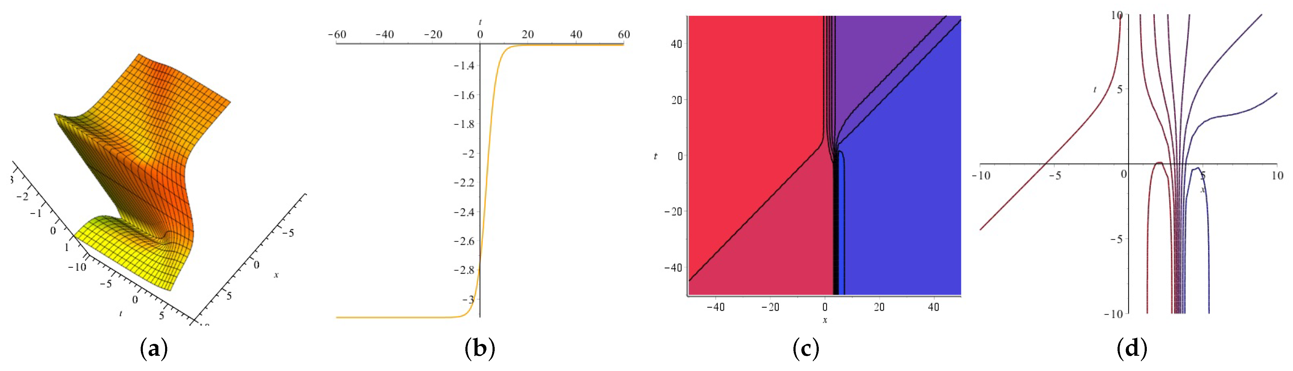
3.1. Mathematical Analysis of the EFM for the Fornberg–Whitham Model

Here, we implement the EFM to obtain analytic and approximate solutions for the special case of the following Gilson–Pickering equation (GPE), i.e., a nonlinear third-order PDE given by [51]
u t A u x x t + 2 B u x u u x x x C u u x D u x u x x = 0 , ( x , t ) ( ϵ , ϵ ) × ( 0 , T ] ,
with
u ( x , 0 ) = ϖ ( x ) , ϵ x ϵ , u ( ϵ , t ) = u ( ϵ , t ) = 0 t ( 0 , T ] ,
where u is an unknown function to be determined, the subscripts denote the partial derivative, the parameters A , D , B and C are arbitrary constants, the function ϖ represents a continuous function, and T is a final time.
We note three special cases for the nonlinear GPE based on particular choices of its parameters:
The Fornberg–Whitham model ( A = 1 , B = 0.5 , C = 1 , and D = 3 in (11)),
The Fuchssteiner-Fokas-Camassa-Holm model ( A = 1 , C = 3 , and D = 2 in (11)),
The Rosenau-Hyman model ( A = 0 , B = 0 , C = 1 , and D = 3 in (11)).
Here, we only consider the first case. Then, by setting A = 1 , B = 0.5 , C = 1 , and D = 3 in the GPE (11) we obtain,
u t u x x t + u x u u x x x + u u x 3 u x u x x = 0 ,
Now, by introducing Ξ defined in (2), then (12) becomes an ODE of the form:
β U α 2 β U + α U α 3 U U + α U U 3 α 3 U U = 0 ,
or
( β + α 3 α 3 U + α U ) U + ( α 2 β α 3 U ) U = 0 .
Integrating Equation (14) and one has:
α 2 U 2 + ( α + β ) U α 3 ( U ) 2 ( α U + β ) α 2 U = 0 .
Based on Equation (4), it is possible to choose different values of c , d , p and q. It is seen that when the equation has multiple solutions (like solitons) the Exp–function method is able to give us these solutions with the aid of using different c , d , p and q. It is worth mentioning that different parameters may lead to equivalent solutions. For convenience, we examine the following cases:
  • Case one ( c = p = 1 , and q = d = 1 ):
Now, Equation (4) reduces to
U ( Ξ ) = a 1 e Ξ + a 0 + a 1 e Ξ b 1 e Ξ + b 0 + b 1 e Ξ ,
Substituting Equation (16) in to Equation (15), and with the help of Maple, we obtain:
α a 1 2 b 1 2 + 2 α a 1 b 1 3 + 2 β a 1 b 1 3 = 0 ,
2 α 3 a 1 2 b 1 b 0 2 α 3 a 1 a 0 b 1 2 + 2 α 2 β a 1 b 1 2 b 0 2 α 2 β a 0 b 1 3 + 2 α a 1 2 b 1 b 0 + 2 α a 1 a 0 b 1 2 + 6 α a 1 b 1 2 b 0 + 2 α a 0 b 1 3 + 6 β a 1 b 1 2 b 0 + 2 β a 0 b 1 3 = 0 ,
8 α 3 a 1 2 b 1 b 1 4 α 3 a 1 2 b 0 2 + 8 α 3 a 1 a 0 b 1 b 0 8 α 3 a 1 a 1 b 1 2 4 α 3 a 0 2 b 1 2 + 8 α 2 β a 1 b 1 2 b 1 8 α 2 β a 1 b 1 3 + 2 α a 1 2 b 1 b 1 + α a 1 2 b 0 2 + 4 α a 1 a 0 b 1 b 0 + 2 α a 1 a 1 b 1 2 + 6 α a 1 b 1 2 b 1 + 6 α a 1 b 1 b 0 2 + α a 0 2 b 1 2 + 6 α a 0 b 1 2 b 0 + 2 α a 1 b 1 3 + 6 β a 1 b 1 2 b 1 + 6 β a 1 b 1 b 0 2 + 6 β a 0 b 1 2 b 0 + 2 β a 1 b 1 3 = 0 ,
14 α 3 a 1 2 b 0 b 1 + 28 α 3 a 1 a 0 b 1 b 1 2 α 3 a 1 a 0 b 0 2 + 4 α 3 a 1 a 1 b 1 b 0 + 2 α 3 a 0 2 b 1 b 0 18 α 3 a 0 a 1 b 1 2 + 4 α 2 β a 1 b 1 b 0 b 1 2 α 2 β a 1 b 0 3 + 10 α 2 β a 0 b 1 2 b 1 + 2 α 2 β a 0 b 1 b 0 2 14 α 2 β a 1 b 1 2 b 0 + 2 α a 1 2 b 0 b 1 + 4 α a 1 a 0 b 1 b 1 + 2 α a 1 a 0 b 0 2 + 4 α a 1 a 1 b 1 b 0 + 12 α a 1 b 1 b 0 b 1 + 2 α a 1 b 0 3 + 2 α a 0 2 b 1 b 0 + 2 α a 0 a 1 b 1 2 + 6 α a 0 b 1 2 b 1 + 6 α a 0 b 1 b 0 2 + 6 α a 1 b 1 2 b 0 + 12 β a 1 b 1 b 0 b 1 + 2 β a 1 b 0 3 + 6 β a 0 b 1 2 b 1 + 6 β a 0 b 1 b 0 2 + 6 β a 1 b 1 2 b 0 = 0 ,
16 α 3 a 1 2 b 1 2 8 α 3 a 1 a 0 b 0 b 1 + 32 α 3 a 1 a 1 b 1 b 1 + 16 α 3 a 0 2 b 1 b 1 8 α 3 a 0 a 1 b 1 b 0 16 α 3 a 1 2 b 1 2 8 α 2 β a 1 b 0 2 b 1 + 16 α 2 β a 0 b 1 b 0 b 1 8 α 2 β a 1 b 1 b 0 2 + α a 1 2 b 1 2 + 4 α a 1 a 0 b 0 b 1 + 4 α a 1 a 1 b 1 b 1 + 2 α a 1 a 1 b 0 2 + 6 α a 1 b 1 b 1 2 + 6 α a 1 b 0 2 b 1 + 2 α a 0 2 b 1 b 1 + α a 0 2 b 0 2 + 4 α a 0 a 1 b 1 b 0 + 12 α a 0 b 1 b 0 b 1 + 2 α a 0 b 0 3 + α a 1 2 b 1 2 + 6 α a 1 b 1 2 b 1 + 6 α a 1 b 1 b 0 2 + 6 β a 1 b 1 b 1 2 + 6 β a 1 b 0 2 b 1 + 12 β a 0 b 1 b 0 b 1 + 2 β a 0 b 0 3 + 6 β a 1 b 1 2 b 1 + 6 β a 1 b 1 b 0 2 = 0 ,
18 α 3 a 1 a 0 b 1 2 + 4 α 3 a 1 a 1 b 0 b 1 + 2 α 3 a 0 2 b 0 b 1 + 28 α 3 a 0 a 1 b 1 b 1 2 α 3 a 0 a 1 b 0 2 14 α 3 a 1 2 b 1 b 0 14 α 2 β a 1 b 0 b 1 2 + 10 α 2 β a 0 b 1 b 1 2 + 2 α 2 β a 0 b 0 2 b 1 + 4 α 2 β a 1 b 1 b 0 b 1 2 α 2 β a 1 b 0 3 + 2 α a 1 a 0 b 1 2 + 4 α a 1 a 1 b 0 b 1 + 6 α a 1 b 0 b 1 2 + 2 α a 0 2 b 0 b 1 + 4 α a 0 a 1 b 1 b 1 + 2 α a 0 a 1 b 0 2 + 6 α a 0 b 1 b 1 2 + 6 α a 0 b 0 2 b 1 + 2 α a 1 2 b 1 b 0 + 12 α a 1 b 1 b 0 b 1 + 2 α a 1 b 0 3 + 6 β a 1 b 0 b 1 2 + 6 β a 0 b 1 b 1 2 + 6 β a 0 b 0 2 b 1 + 12 β a 1 b 1 b 0 b 1 + 2 β a 1 b 0 3 = 0 ,
8 α 3 a 1 a 1 b 1 2 4 α 3 a 0 2 b 1 2 + 8 α 3 a 0 a 1 b 0 b 1 + 8 α 3 a 1 2 b 1 b 1 4 α 3 a 1 2 b 0 2 8 α 2 β a 1 b 1 3 + 8 α 2 β a 1 b 1 b 1 2 + 2 α a 1 a 1 b 1 2 + 2 α a 1 b 1 3 + α a 0 2 b 1 2 + 4 α a 0 a 1 b 0 b 1 + 6 α a 0 b 0 b 1 2 + 2 α a 1 2 b 1 b 1 + α a 1 2 b 0 2 + 6 α a 1 b 1 b 1 2 + 6 α a 1 b 0 2 b 1 + 2 β a 1 b 1 3 + 6 β a 0 b 0 b 1 2 + 6 β a 1 b 1 b 1 2 + 6 β a 1 b 0 2 b 1 = 0 ,
Solving the system of algebraic equations, simultaneously yields:
β = β , b 1 = b 1 , a 1 = 0 , b 0 = b 0 , a 0 = 0 , b 1 = b 1 , a 1 = 0 , ,
β = β , b 1 = 0 , a 1 = a 1 , b 0 = 0 , a 0 = a 0 , b 1 = 0 , a 1 = a 1 ,
β = β , b 1 = 0 , a 1 = 0 , b 0 = 0.5 α a 0 β + α , a 0 = a 0 , b 1 = 0.5 a 1 α β + α a 1 = a 1 ,
β = β , b 1 = 0 , a 1 = 0 , b 0 = 0 , a 0 = 0 , b 1 = b 1 , a 1 = a 1 ,
β = α ( 2 α 2 1 ) α 2 1 , b 1 = b 1 , a 1 = 2 b 1 α 2 α 2 1 , b 0 = b 0 , a 0 = 2 α 2 b 0 α 2 1 , b 1 = 0 , a 1 = 0 ,
β = α α 2 1 , b 1 = 0 , a 1 = 0 , b 0 = b 0 , a 0 = 0 , b 1 = b 1 , a 1 = 6 b 1 α 2 4 α 4 5 α 2 + 1 ,
and putting our obtained results into Equation (16), we obtain the following generalized solution of Equation (15) as:
U ( Ξ ) = 0 ,
U ( Ξ ) = a 1 e Ξ + a 0 0.5 a 1 α β + α e Ξ 0.5 α a 0 β + α ,
U ( Ξ ) = 2 α 2 b 0 α 2 1 + 2 b 1 α 2 α 2 1 e Ξ b 0 + b 1 e Ξ ,
U ( Ξ ) = 6 b 1 α 2 4 α 4 5 α 2 + 1 e Ξ b 1 e Ξ + b 0 ,
Substituting Equation (8) into our obtained results we obtain:
u ( x , t ) = 0 ,
u ( x , t ) = a 1 e α x + β t + a 0 0.5 a 1 α β + α e α x + β t 0.5 α a 0 β + α ,
u ( x , t ) = 2 α 2 b 0 α 2 1 + 2 b 1 α 2 α 2 1 e ( α x α ( 2 α 2 1 ) α 2 1 t ) b 0 + b 1 e ( α x α ( 2 α 2 1 ) α 2 1 t ) ,
u ( x , t ) = 6 b 1 α 2 4 α 4 5 α 2 + 1 e α x + α α 2 1 t b 1 e α x + α α 2 1 t + b 0 ,
Figure 1, displays the 3D and 2D with the plots of Equation (18), for α = 0.5 , b 0 = 5 , and b 1 = 4.5 .
  • Case two ( c = p = 2 , and q = d = 2 ):
Here, Equation (4) reduces to
U ( Ξ ) = a 2 e 2 Ξ + a 1 e Ξ + a 0 + a 1 e Ξ + a 2 e 2 Ξ b 2 e 2 Ξ + b 1 e Ξ + b 0 + b 1 e Ξ + b 2 e 2 Ξ .
There are some free parameters in Equation (20), we set b 1 = 0 , and b 1 = 0 , for convenience, and the trial function, Equation (20) is simplified as
U ( Ξ ) = a 2 e 2 Ξ + a 1 e Ξ + a 0 + a 1 e Ξ + a 2 e 2 Ξ b 2 e 2 Ξ + b 0 + b 2 e 2 Ξ .
Substituting Equation (21) into Equation (15), and with Maple, we obtain:
1 2 α a 2 2 b 2 2 + α a 2 b 2 3 + β a 2 b 2 3 = 0 ,
α 3 a 2 a 1 b 2 2 α 2 β a 1 b 2 3 + α a 2 a 1 b 2 2 + α a 1 b 2 3 + β a 1 b 2 3 = 0 ,
α a 0 b 2 3 + β a 0 b 2 3 + 1 2 α a 1 2 b 2 2 2 α 3 a 1 2 b 2 2 + 4 α 2 β a 2 b 2 2 b 0 + 4 α 3 a 2 2 b 2 b 0 4 α 3 a 0 b 2 2 a 2 4 α 2 β a 0 b 2 3 + 3 α a 2 b 2 2 b 0 + 3 β a 2 b 2 2 b 0 + α a 2 2 b 2 b 0 + α a 2 a 0 b 2 2 = 0 ,
14 α 3 a 2 a 1 b 2 b 0 9 α 3 a 2 a 1 b 2 2 9 α 3 a 1 a 0 b 2 2 + 5 α 2 β a 1 b 2 2 b 0 9 α 2 β a 1 b 2 3 + 2 α a 2 a 1 b 2 b 0 + α a 2 a 1 b 2 2 + α a 1 a 0 b 2 2 + 3 α a 1 b 2 2 b 0 + α a 1 b 2 3 + 3 β a 1 b 2 2 b 0 + β a 1 b 2 3 = 0 ,
α a 2 b 2 3 + β a 2 b 2 3 8 α 3 a 2 2 b 0 2 8 α 3 a 0 2 b 2 2 + 1 2 α a 2 2 b 0 2 + 1 2 α a 0 2 b 2 2 + 16 α 3 a 2 a 0 b 2 b 0 + 16 α 2 β a 2 b 2 2 b 2 + 2 α a 2 a 0 b 2 b 0 + 16 α 3 a 2 2 b 2 b 2 16 α 3 a 2 b 2 2 a 2 + 8 α 3 a 1 2 b 2 b 0 16 α 3 a 1 b 2 2 a 1 16 α 2 β a 2 b 2 3 + 3 α a 2 b 2 2 b 2 + 3 α a 2 b 2 b 0 2 + 3 α a 0 b 2 2 b 0 + 3 β a 2 b 2 2 b 2 + 3 β a 2 b 2 b 0 2 + 3 β a 0 b 2 2 b 0 + α a 2 2 b 2 b 2 + α a 2 a 2 b 2 2 + α a 1 2 b 2 b 0 + α a 1 a 1 b 2 2 = 0 ,
46 α 3 a 2 a 1 b 2 b 2 9 α 3 a 2 a 1 b 0 2 + 14 α 3 a 2 a 1 b 2 b 0 + 14 α 3 a 1 a 0 b 2 b 0 25 α 3 a 1 a 2 b 2 2 25 α 3 a 0 a 1 b 2 2 + 21 α 2 β a 1 b 2 2 b 2 + 5 α 2 β a 1 b 2 b 0 2 11 α 2 β a 1 b 2 2 b 0 + 2 α a 2 a 1 b 2 b 2 + α a 2 a 1 b 0 2 + 2 α a 2 a 1 b 2 b 0 + 2 α a 1 a 0 b 2 b 0 + α a 1 a 2 b 2 2 + 3 α a 1 b 2 2 b 2 + 3 α a 1 b 2 b 0 2 + α a 0 a 1 b 2 2 + 3 α a 1 b 2 2 b 0 + 3 β a 1 b 2 2 b 2 + 3 β a 1 b 2 b 0 2 + 3 β a 1 b 2 2 b 0 = 0 ,
2 α a 2 a 0 b 2 b 2 + 2 α a 2 a 2 b 2 b 0 + 6 α a 2 b 2 b 0 b 2 + 2 α a 1 a 1 b 2 b 0 + 6 β a 2 b 2 b 0 b 2 + 56 α 3 a 0 b 2 a 2 b 2 + 8 α 3 a 2 a 2 b 2 b 0 + 8 α 3 a 1 a 1 b 2 b 0 + 20 α 2 β a 0 b 2 2 b 2 + 4 α 2 β a 0 b 2 b 0 2 28 α 2 β a 2 b 2 2 b 0 + α a 2 2 b 0 b 2 + α a 2 a 0 b 0 2 + α a 1 2 b 2 b 2 + α a 0 2 b 2 b 0 + α a 0 a 2 b 2 2 + 3 α a 0 b 2 2 b 2 + 3 α a 0 b 2 b 0 2 + 3 α a 2 b 2 2 b 0 28 α 3 a 2 2 b 0 b 2 4 α 3 a 2 a 0 b 0 2 + 28 α 3 a 1 2 b 2 b 2 + 4 α 3 a 0 2 b 2 b 0 36 α 3 a 2 b 2 2 a 0 4 α 2 β a 2 b 0 3 + 3 β a 0 b 2 2 b 2 + 3 β a 0 b 2 b 0 2 + 3 β a 2 b 2 2 b 0 + 8 α 2 β a 2 b 2 b 0 b 2 + α a 2 b 0 3 + β a 2 b 0 3 2 α 3 a 1 2 b 0 2 18 α 3 a 1 2 b 2 2 = 0 ,
34 α 3 a 2 a 1 b 0 b 2 + 62 α 3 a 2 a 1 b 2 b 2 α 3 a 2 a 1 b 0 2 + 62 α 3 a 1 a 0 b 2 b 2 α 3 a 1 a 0 b 0 2 2 α 3 a 1 a 2 b 2 b 0 2 α 3 a 0 a 1 b 2 b 0 49 α 3 a 1 a 2 b 2 2 + 26 α 2 β a 1 b 2 b 0 b 2 α 2 β a 1 b 0 3 + 13 α 2 β a 1 b 2 2 b 2 3 α 2 β a 1 b 2 b 0 2 + 2 α a 2 a 1 b 0 b 2 + 2 α a 2 a 1 b 2 b 2 + α a 2 a 1 b 0 2 + 2 α a 1 a 0 b 2 b 2 + α a 1 a 0 b 0 2 + 2 α a 1 a 2 b 2 b 0 + 6 α a 1 b 2 b 0 b 2 + α a 1 b 0 3 + 2 α a 0 a 1 b 2 b 0 + α a 1 a 2 b 2 2 + 3 α a 1 b 2 2 b 2 + 3 α a 1 b 2 b 0 2 + 6 β a 1 b 2 b 0 b 2 + β a 1 b 0 3 + 3 β a 1 b 2 2 b 2 + 3 β a 1 b 2 b 0 2 = 0 ,
1 2 α a 0 2 b 0 2 + 1 2 α a 2 2 b 2 2 32 α 3 a 2 2 b 2 2 + α a 0 b 0 3 32 α 3 a 2 2 b 2 2 + 1 2 α a 2 2 b 2 2 + β a 0 b 0 3 16 α 3 a 0 a 2 b 2 b 0 + 64 α 3 a 2 b 2 a 2 b 2 + 64 α 3 a 1 b 2 a 1 b 2 16 α 2 β a 2 b 0 2 b 2 16 α 2 β a 2 b 2 b 0 2 16 α 3 a 2 a 0 b 0 b 2 + 2 α a 2 a 0 b 0 b 2 + 2 α a 2 a 2 b 2 b 2 + 2 α a 1 a 1 b 2 b 2 + 2 α a 0 a 2 b 2 b 0 + 6 α a 0 b 2 b 0 b 2 + 6 β a 0 b 2 b 0 b 2 + 32 α 2 β a 0 b 2 b 0 b 2 + 3 α a 2 b 2 b 0 2 + 3 β a 2 b 2 b 2 2 + 3 β a 2 b 0 2 b 2 + 3 β a 2 b 2 2 b 2 + 3 β a 2 b 2 b 0 2 8 α 3 a 1 2 b 0 b 2 + 32 α 3 a 0 2 b 2 b 2 8 α 3 a 1 2 b 2 b 0 + 3 α a 2 b 2 b 2 2 + 3 α a 2 b 0 2 b 2 + 3 α a 2 b 2 2 b 2 + α a 1 2 b 0 b 2 + α a 1 a 1 b 0 2 + α a 0 2 b 2 b 2 + α a 1 2 b 2 b 0 + α a 2 a 2 b 0 2 = 0 ,
49 α 3 a 2 a 1 b 2 2 2 α 3 a 2 a 1 b 0 b 2 2 α 3 a 1 a 0 b 0 b 2 + 62 α 3 a 1 a 2 b 2 b 2 α 3 a 1 a 2 b 0 2 + 62 α 3 a 0 a 1 b 2 b 2 α 3 a 0 a 1 b 0 2 34 α 3 a 1 a 2 b 2 b 0 + 13 α 2 β a 1 b 2 b 2 2 3 α 2 β a 1 b 0 2 b 2 + 26 α 2 β a 1 b 2 b 0 b 2 α 2 β a 1 b 0 3 + α a 2 a 1 b 2 2 + 2 α a 2 a 1 b 0 b 2 + 2 α a 1 a 0 b 0 b 2 + 2 α a 1 a 2 b 2 b 2 + α a 1 a 2 b 0 2 + 3 α a 1 b 2 b 2 2 + 3 α a 1 b 0 2 b 2 + 2 α a 0 a 1 b 2 b 2 + α a 0 a 1 b 0 2 + 2 α a 1 a 2 b 2 b 0 + 6 α a 1 b 2 b 0 b 2 + α a 1 b 0 3 + 3 β a 1 b 2 b 2 2 + 3 β a 1 b 0 2 b 2 + 6 β a 1 b 2 b 0 b 2 + β a 1 b 0 3 = 0 ,
36 α 3 a 0 b 2 2 a 2 + 4 α 3 a 0 2 b 0 b 2 4 α 3 a 0 a 2 b 0 2 + 28 α 3 a 1 2 b 2 b 2 28 α 3 a 2 2 b 2 b 0 4 α 2 β a 2 b 0 3 + 2 α a 0 a 2 b 2 b 2 + 6 α a 2 b 2 b 0 b 2 + 6 β a 2 b 2 b 0 b 2 + 2 α a 2 a 2 b 0 b 2 + 2 α a 1 a 1 b 0 b 2 + 8 α 3 a 2 a 2 b 0 b 2 + 8 α 3 a 1 a 1 b 0 b 2 + 56 α 3 a 2 b 2 a 0 b 2 28 α 2 β a 2 b 0 b 2 2 + 20 α 2 β a 0 b 2 b 2 2 + 4 α 2 β a 0 b 0 2 b 2 + 3 α a 2 b 0 b 2 2 + 3 α a 0 b 2 b 2 2 + 3 α a 0 b 0 2 b 2 + 3 β a 2 b 0 b 2 2 + 3 β a 0 b 2 b 2 2 + α a 2 a 0 b 2 2 + α a 0 2 b 0 b 2 + α a 0 a 2 b 0 2 + α a 1 2 b 2 b 2 + α a 2 2 b 2 b 0 + 3 β a 0 b 0 2 b 2 + 8 α 2 β a 2 b 2 b 0 b 2 + α a 2 b 0 3 + β a 2 b 0 3 18 α 3 a 1 2 b 2 2 2 α 3 a 1 2 b 0 2 + 1 2 α a 1 2 b 2 2 + 1 2 α a 1 2 b 0 2 = 0 ,
25 α 3 a 2 a 1 b 2 2 25 α 3 a 1 a 0 b 2 2 + 14 α 3 a 1 a 2 b 0 b 2 + 14 α 3 a 0 a 1 b 0 b 2 + 46 α 3 a 1 a 2 b 2 b 2 9 α 3 a 1 a 2 b 0 2 11 α 2 β a 1 b 0 b 2 2 + 21 α 2 β a 1 b 2 b 2 2 + 5 α 2 β a 1 b 0 2 b 2 + α a 2 a 1 b 2 2 + α a 1 a 0 b 2 2 + 2 α a 1 a 2 b 0 b 2 + 3 α a 1 b 0 b 2 2 + 2 α a 0 a 1 b 0 b 2 + 2 α a 1 a 2 b 2 b 2 + α a 1 a 2 b 0 2 + 3 α a 1 b 2 b 2 2 + 3 α a 1 b 0 2 b 2 + 3 β a 1 b 0 b 2 2 + 3 β a 1 b 2 b 2 2 + 3 β a 1 b 0 2 b 2 = 0 ,
α a 2 b 2 3 + β a 2 b 2 3 8 α 3 a 0 2 b 2 2 8 α 3 a 2 2 b 0 2 + 1 2 α a 0 2 b 2 2 + 1 2 α a 2 2 b 0 2 + 16 α 3 a 0 a 2 b 0 b 2 + 16 α 2 β a 2 b 2 b 2 2 + 2 α a 0 a 2 b 0 b 2 + 3 β a 2 b 0 2 b 2 16 α 3 a 2 b 2 2 a 2 16 α 3 a 1 b 2 2 a 1 + 8 α 3 a 1 2 b 0 b 2 + 16 α 3 a 2 2 b 2 b 2 16 α 2 β a 2 b 2 3 + 3 α a 0 b 0 b 2 2 + 3 α a 2 b 2 b 2 2 + 3 α a 2 b 0 2 b 2 + 3 β a 0 b 0 b 2 2 + 3 β a 2 b 2 b 2 2 + α a 1 2 b 0 b 2 + α a 2 2 b 2 b 2 + α a 2 a 2 b 2 2 + α a 1 a 1 b 2 2 = 0 .
Solving the system of algebraic equations simultaneously yields:
{ β = α 4 α 2 1 , b 2 = 0 , a 2 = 0 , a 1 = 0 , b 0 = b 0 , a 0 = 0 , b 2 = 1 24 a 2 ( 64 α 4 20 α 2 + 1 ) α 2 , a 2 = a 2 , a 1 = 0 , } ,
β = β , b 2 = b 2 , a 2 = 0 , a 1 = 0 , b 0 = b 0 , a 0 = 0 , a 1 = 0 , b 2 = b 2 , a 2 = 0 , ,
β = β , b 2 = 0 , a 2 = 0 , a 1 = 0 , b 0 = 0 , a 0 = 0 , a 1 = a 1 , b 2 = b 2 , a 2 = a 2 ,
β = 1 2 α ( a 0 + 2 b 0 ) b 0 , b 2 = 0 , a 2 = 0 , a 1 = 0 , b 0 = b 0 , a 0 = a 0 , a 1 = 0 , b 2 = b 2 , a 2 = a 0 b 2 b 0 ,
{ β = α ( 8 α 2 1 ) 4 α 2 1 , b 2 = 0 , a 2 = 0 , a 1 = 0 , b 0 = 1 8 a 0 ( 4 α 2 1 ) α 2 , a 0 = a 0 , a 1 = 0 , b 2 = 1 16 a 2 ( 64 α 4 20 α 2 + 1 ) α 2 ( 8 α 2 + 1 ) , a 2 = a 2 } ,
β = 1 2 α ( a 2 + 2 b 2 ) b 2 , b 2 = b 2 , a 2 = a 2 b 2 b 2 , a 1 = 0 , , b 0 = 0 , a 0 = 0 , a 1 = 0 , b 2 = b 2 , a 2 = a 2 , ,
β = 1 2 α ( a 2 + 2 b 2 ) b 2 , b 2 = b 2 , a 2 = a 2 , a 1 = 0 , b 0 = b 0 , b 0 = b 0 , a 1 = 0 , b 2 = b 2 a 2 = a 2 b 2 b 2 ,
β = β , b 2 = 0 , a 2 = a 2 , a 1 = a 1 , b 0 = 0 , a 0 = a 0 , a 1 = a 1 , b 2 = 0 , a 2 = a 2 ,
and putting our obtained results into Equation (21), we obtain the generalized solution of Equation (15) as follows:
U ( Ξ ) = a 2 e 2 Ξ 1 24 a 2 ( 64 α 4 20 α 2 + 1 ) α 2 e 2 Ξ + b 0 ,
U ( Ξ ) = 0 ,
U ( Ξ ) = a 2 e 2 Ξ + a 1 e Ξ b 2 e 2 Ξ ,
U ( Ξ ) = a 0 b 2 b 0 e 2 Ξ + a 0 b 2 e 2 Ξ + b 0 ,
U ( Ξ ) = a 2 e 2 Ξ + a 0 1 16 a 2 ( 64 α 4 20 α 2 + 1 ) α 2 ( 8 α 2 + 1 ) e 2 Ξ + 1 8 a 0 ( 4 α 2 1 ) α 2 ,
U ( Ξ ) = a 2 e 2 Ξ + a 2 b 2 b 2 e 2 Ξ b 2 e 2 Ξ + b 2 e 2 Ξ ,
U ( Ξ ) = a 2 b 2 b 2 e 2 Ξ + a 2 b 0 b 2 + a 2 e 2 Ξ b 2 e 2 Ξ + b 0 + b 2 e 2 Ξ ,
and putting Equation (8) into our obtained results we obtain:
u ( x , t ) = a 2 e 2 ( α x + α 4 α 2 1 t ) 1 24 a 2 ( 64 α 4 20 α 2 + 1 ) α 2 e 2 ( α x + α 4 α 2 1 t ) + b 0 ,
u ( x , t ) = 0 ,
u ( x , t ) = a 2 e 2 ( α x + β t ) + a 1 e α x + β t b 2 e 2 ( α x + β t ) ,
u ( x , t ) = a 0 b 2 b 0 e 2 ( α x 1 2 α ( a 0 + 2 b 0 ) b 0 t ) + a 0 b 2 e 2 ( α x 1 2 α ( a 0 + 2 b 0 ) b 0 t ) + b 0 ,
u ( x , t ) = a 2 e 2 ( α x α ( 8 α 2 1 ) 4 α 2 1 t ) + a 0 1 16 a 2 ( 64 α 4 20 α 2 + 1 ) α 2 ( 8 α 2 + 1 ) e 2 ( α x α ( 8 α 2 1 ) 4 α 2 1 t ) + 1 8 a 0 ( 4 α 2 1 ) α 2 ,
u ( x , t ) = a 2 e 2 ( α x 1 2 α ( a 2 + 2 b 2 ) b 2 t ) + a 2 b 2 b 2 e 2 ( α x 1 2 α ( a 2 + 2 b 2 ) b 2 t ) b 2 e 2 ( α x 1 2 α ( a 2 + 2 b 2 ) b 2 t ) + b 2 e 2 ( α x 1 2 α ( a 2 + 2 b 2 ) b 2 t ) ,
u ( x , t ) = a 2 b 2 b 2 e 2 ( α x 1 2 α ( a 2 + 2 b 2 ) b 2 t ) + a 2 b 0 b 2 + a 2 e 2 ( α x 1 2 α ( a 2 + 2 b 2 ) b 2 t ) b 2 e 2 ( α x 1 2 α ( a 2 + 2 b 2 ) b 2 t ) + b 0 + b 2 e 2 ( α x 1 2 α ( a 2 + 2 b 2 ) b 2 t ) .
Figure 2 displays the 3D and 2D with the plots of Equation (26), for α = 0.5 , a 2 = 2.5 , b 2 = 3.5 , and b 2 = 3 . And also, Figure 3 displays the 3D and 2D with the plots of Equation (27), for α = 0.5 , a 2 = 3 , b 2 = 3.5 , and b 0 = 5 .
  • Case three ( c = p = 2 , and q = d = 1 ):
Here, Equation (4) reduces to
U ( Ξ ) = a 2 e 2 Ξ + a 1 e Ξ + a 0 + a 1 e Ξ b 2 e 2 Ξ + b 1 e Ξ + b 0 + b 1 e Ξ .
By the same manipulation as illustrated above, we obtain:
β = β , b 1 = b 1 , a 1 = 0 , b 0 = b 0 , a 0 = 0 , b 1 = b 1 , a 1 = 0 , a 2 = 0 , b 2 = b 2 ,
β = α α 2 1 , b 1 = 0 , a 1 = 0 , b 0 = 0 , a 0 = 0 , b 1 = b 1 , a 1 = 0 , b 2 = b 2 , a 2 = a 2 ,
{ β = α 4 α 2 1 , b 1 = 0 , a 1 = 0 , b 0 = b 0 , b 1 = 0 , a 0 = 0 , a 1 = 0 , b 2 = 1 24 a 2 ( 64 α 4 20 α 2 + 1 ) α 2 , a 2 = a 2 } ,
β = β , b 1 = 0 , a 1 = 0 , b 0 = 0 , a 0 = 0 , b 1 = 0 , a 1 = a 1 , b 2 = b 2 , a 2 = a 2 ,
β = 1 2 α ( a 1 + 2 b 1 ) b 1 , b 1 = 0 , a 1 = 0 , b 0 = 0 , a 0 = 0 , b 1 = b 1 , a 1 = a 1 , b 2 = b 2 , a 2 = a 1 b 2 b 1 ,
β = α ( 2 α 2 1 ) α 2 1 , b 1 = 0 , a 1 = 0 , b 0 = 0 , a 0 = 0 , b 1 = 1 2 a 1 ( α 2 1 ) α 2 , a 1 = a 1 , b 2 = b 2 , a 2 = a 2 ,
{ β = α ( 8 α 2 1 ) 4 α 2 1 , b 1 = 0 , a 1 = 0 , b 0 = 1 8 a 0 ( 4 α 2 1 ) α 2 , a 0 = a 0 , b 1 = 0 , a 1 = 0 , b 2 = 1 16 a 2 ( 64 α 4 20 α 2 + 1 ) α 2 ( 8 α 2 + 1 ) , a 2 = a 2 } ,
β = 1 2 α ( a 0 + 2 b 0 ) b 0 , b 1 = 0 , a 1 = 0 , b 0 = b 0 , a 0 = a 0 , b 1 = b 1 , a 1 = a 0 b 1 b 0 , b 2 = b 2 , a 2 = a 0 b 2 b 0 ,
β = β , b 1 = 0 , a 1 = a 1 , b 0 = 0 , a 0 = a 0 , b 1 = 0 , a 1 = a 1 , b 2 = 0 , a 2 = a 2 ,
β = 1 2 α ( a 2 + 2 b 2 ) b 2 , b 1 = b 1 , a 1 = a 2 b 1 b 2 , b 0 = 0 , a 0 = 0 , b 1 = 0 , a 1 = 0 , b 2 = b 2 , a 2 = a 2 ,
{ β = 1 2 α ( a 1 + 2 b 1 ) b 1 , b 1 = b 1 , a 1 = a 1 , b 0 = b 0 , a 0 = a 1 b 0 b 1 , b 1 = b 1 , a 1 = a 1 b 1 b 1 , b 2 = b 2 , a 2 = a 1 b 2 b 1 } .
and putting our obtained results into Equation (28), we obtain the following generalized solution of Equation (15) as:
U ( Ξ ) = 0 ,
U ( Ξ ) = a 2 e 2 Ξ b 2 e 2 Ξ + b 1 e Ξ ,
U ( Ξ ) = a 2 e 2 Ξ 1 24 a 2 ( 64 α 4 20 α 2 + 1 ) α 2 e 2 Ξ + b 0 ,
U ( Ξ ) = a 2 e 2 Ξ + a 1 e Ξ b 2 e 2 Ξ ,
U ( Ξ ) = a 1 b 2 b 1 e 2 Ξ + a 1 e Ξ b 2 e 2 Ξ + b 1 e Ξ ,
U ( Ξ ) = a 2 e 2 Ξ + a 1 e Ξ b 2 e 2 Ξ + 1 2 a 1 ( α 2 1 ) α 2 e Ξ ,
U ( Ξ ) = a 2 e 2 Ξ + a 0 1 16 a 2 ( 64 α 4 20 α 2 + 1 ) α 2 ( 8 α 2 + 1 ) e 2 Ξ + 1 8 a 0 ( 4 α 2 1 ) α 2 ,
U ( Ξ ) = a 0 b 2 b 0 e 2 Ξ + a 0 b 1 b 0 e Ξ b 2 e 2 Ξ + b 1 e Ξ + b 0 ,
U ( Ξ ) = a 2 e 2 Ξ + a 2 b 1 b 2 e Ξ b 2 e 2 Ξ + b 1 e Ξ ,
U ( Ξ ) = a 1 b 2 b 1 e 2 Ξ + a 1 b 1 b 1 e Ξ + a 1 b 0 b 1 + a 1 e Ξ b 2 e 2 Ξ + b 1 e Ξ + b 0 + b 1 e Ξ .
Substituting Equation (8) into our obtained results and we obtain:
u ( x , t ) = 0 ,
u ( x , t ) = a 2 e 2 ( α x + α α 2 1 t ) b 2 e 2 ( α x + α α 2 1 t ) + b 1 e α x + α α 2 1 t ,
u ( x , t ) = a 2 e 2 ( α x + α 4 α 2 1 t ) 1 24 a 2 ( 64 α 4 20 α 2 + 1 ) α 2 e 2 ( α x + α 4 α 2 1 t ) + b 0 ,
u ( x , t ) = a 2 e 2 ( α x + β t ) + a 1 e α x + β t b 2 e 2 ( α x + β t ) ,
u ( x , t ) = a 1 b 2 b 1 e 2 ( α x 1 2 α ( a 1 + 2 b 1 ) b 1 t ) + a 1 e α x 1 2 α ( a 1 + 2 b 1 ) b 1 t b 2 e 2 ( α x 1 2 α ( a 1 + 2 b 1 ) b 1 t ) + b 1 e α x 1 2 α ( a 1 + 2 b 1 ) b 1 t ,
u ( x , t ) = a 2 e 2 ( α x α ( 2 α 2 1 ) α 2 1 t ) + a 1 e α x α ( 2 α 2 1 ) α 2 1 t b 2 e 2 ( α x α ( 2 α 2 1 ) α 2 1 t ) + 1 2 a 1 ( α 2 1 ) α 2 e α x α ( 2 α 2 1 ) α 2 1 t ,
u ( x , t ) = a 2 e 2 ( α x α ( 8 α 2 1 ) 4 α 2 1 t ) + a 0 1 16 a 2 ( 64 α 4 20 α 2 + 1 ) α 2 ( 8 α 2 + 1 ) e 2 ( α x α ( 8 α 2 1 ) 4 α 2 1 t ) + 1 8 a 0 ( 4 α 2 1 ) α 2 ,
u ( x , t ) = a 0 b 2 b 0 e 2 ( α x 1 2 α ( a 0 + 2 b 0 ) b 0 t ) + a 0 b 1 b 0 e α x 1 2 α ( a 0 + 2 b 0 ) b 0 t b 2 e 2 ( α x 1 2 α ( a 0 + 2 b 0 ) b 0 t ) + b 1 e α x 1 2 α ( a 0 + 2 b 0 ) b 0 t + b 0 ,
u ( x , t ) = a 2 e 2 ( α x 1 2 α ( a 2 + 2 b 2 ) b 2 t ) + a 2 b 1 b 2 e ( α x 1 2 α ( a 2 + 2 b 2 ) b 2 t ) b 2 e 2 ( α x 1 2 α ( a 2 + 2 b 2 ) b 2 t ) + b 1 e ( α x 1 2 α ( a 2 + 2 b 2 ) b 2 t ) ,
u ( x , t ) = a 1 b 2 b 1 e 2 ( α x 1 2 α ( a 1 + 2 b 1 ) b 1 t ) + a 1 b 1 b 1 e α x 1 2 α ( a 1 + 2 b 1 ) b 1 t + a 1 b 0 b 1 + a 1 e ( α x 1 2 α ( a 1 + 2 b 1 ) b 1 t ) b 2 e 2 ( α x 1 2 α ( a 1 + 2 b 1 ) b 1 t ) + b 1 e α x 1 2 α ( a 1 + 2 b 1 ) b 1 t + b 0 + b 1 e ( α x 1 2 α ( a 1 + 2 b 1 ) b 1 t ) .
By modelling the propogation of waves in crystal lattice theory and plasma physics, we were able to present analytical research on their propogation. Here, we have considered only three case for the values of the positive integers c = d = p = q = 1 , c = d = p = q = 2 , and c = p = 2 , d = q = 1 . If we consider the other values of c , p , d , q , then, we can obtain more general solutions, which shows the novelty of our work. All the exact solutions attained in this article have been checked by using Maple 18 to the Fornberg–Whitham model and found to be appropriate. It has been shown that the applied method is effective because it provides a lot of new solutions. The solutions obtained by Bariza Boutarfa et al. [52] are re-derived when parameters are given some specific values.
We can similarly have a coth method (CHM) or tanh method (THM) for obtaining the exact solutions of NPDEs. The obtained results in [53] prove that the EFM and THM are effective and simple techniques to solve NPDEs, and by comparison, the authors detect that the EFM is more effective in finding exact solutions than THM. Note, EFM is concerned about travelling wave solutions to NPDEs. It is known that there exist multiple wave solutions to NPDEs, for example, multi-soliton solutions to many physically important equations like the Toda lattice equation, Hirota bilinear equations, the KdV equation and multiple periodic wave solutions to the Boussinesq equation. In the following subsection we formulate a solution algorithm for calculating multiple wave solutions to a (2+1)–dimensional NPDE.

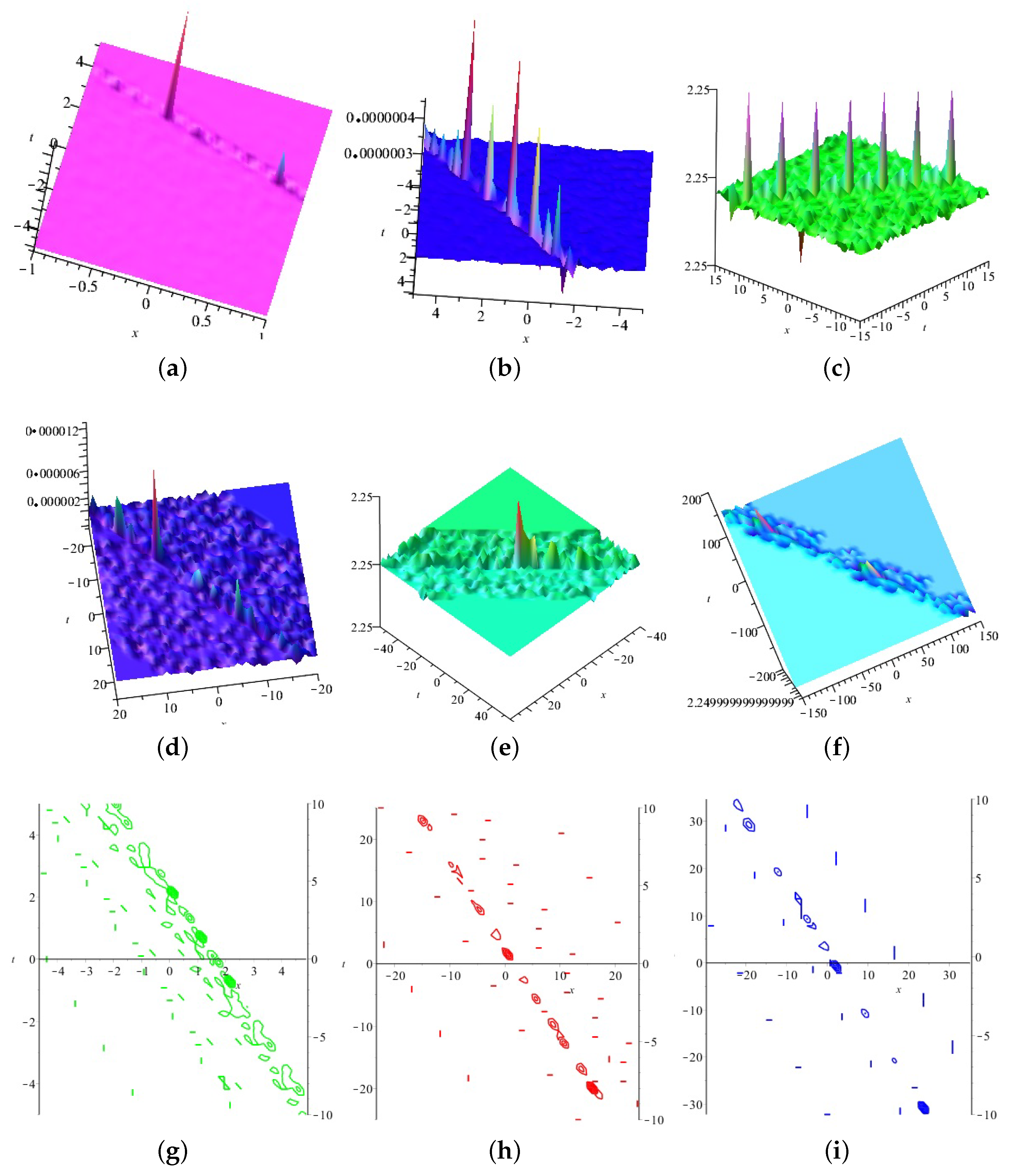
3.2. Mathematical Analysis of MEFM for a (2+1)-Dimensional Equation

In this subsection, we use the MEFM to obtain novel analytical solutions for the following (2+1)-dimensional equation [54]
u y t + u x x x t + 3 u x u x t + 3 u x x u t = 0 .
  • One wave solutions for (38):
First, present Ξ 1 = Ξ 1 ( x , y , t ) as
Ξ 1 = ϖ 1 exp ( S 1 x + R 1 y ω 1 t ) ,
where ϖ 1 , S 1 , R 1 , and ω 1 are constants. Now, Ξ 1 has the following relations
Ξ 1 , x = S 1 Ξ 1 , Ξ 1 , y = R 1 Ξ 1 , Ξ 1 , t = ω 1 Ξ 1 .
Therefore, we assume
H ( Ξ 1 ) = Q 0 + Q 1 Ξ 1 ,
K ( Ξ 1 ) = P 0 + P 1 Ξ 1 ,
where P 0 , P 1 , Q 0 , and Q 1 are fixed to be determined from (38). Thus, we obtain
u ( x , t ) = K ( Ξ 1 ) H ( Ξ 1 ) = P 0 + P 1 Ξ 1 Q 0 + Q 1 Ξ 1 .
By inserting (43) in (38), we have:
P 1 = Q 1 P 0 Q 0 , ω 1 : arbitrary .
Therefore, we obtain
u ( x , t ) = P 0 + Q 1 P 0 Q 0 exp ( S 1 x + R 1 y ω 1 t ) Q 0 + Q 1 exp ( S 1 x + R 1 y ω 1 t ) .
Equation (44) is displayed in Figure 4 for S 1 = Q 1 = 0.70 , R 1 = P 0 = 0.90 , Q 0 = 0.40 , ω 1 = 0.5 , (a) is three dimensional with y = z = 2 , (b) exploits the t-curve with x = y = z = 2 , and (c) and (d) are the contour plots.
  • Two wave solutions for (38):
Now, consider Ξ i = Ξ i ( x , y , t ) , i = 1 , 2 , as
Ξ i = ϖ i exp ( S i x + R i y ω i t ) , i = 1 , 2
where S i ,   ϖ i ,   ω i , and R i , are fixed. We have
Ξ i , t = ω i Ξ i , Ξ i , y = R i Ξ 1 , Ξ i , x = S i Ξ i , i = 1 , 2 .
Therefore, we assume
K ( Ξ 1 , Ξ 2 ) = 2 ( S 1 Ξ 1 + S 2 Ξ 2 + P 12 ( S 1 + S 2 ) Ξ 1 Ξ 2 ) ,
H ( Ξ 1 , Ξ 2 ) = 1 + Ξ 1 + Ξ 2 + P 12 Ξ 1 Ξ 2 ,
where P 12 is a constant to be determined from (38). Therefore, we have
u ( x , t ) = 2 ( S 1 Ξ 1 + S 2 Ξ 2 + P 12 ( S 1 + S 2 ) Ξ 1 Ξ 2 ) 1 + Ξ 1 + Ξ 2 + P 12 Ξ 1 Ξ 2 .
Now, by inserting (49) into (38) and solving the system of linear equations, we have:
P 12 : arbitrary , S 1 = ( R 1 ) 1 3 ( 1 ) 1 3 , S 2 = ( R 2 ) 1 3 ( 1 ) 1 3 , S 3 : arbitrary , ω 2 : arbitrary , ω 1 = ω 2 [ 2 ( R 1 ) 2 3 ( 1 ) 1 3 ( R 2 ) 2 3 P 12 R 1 ( R 2 ) 1 3 ( 1 ) 1 3 + ( R 1 ) 1 3 ( 1 ) 1 3 P 12 R 2 R 1 ( R 2 ) 1 3 ( 1 ) 1 3 ( R 1 ) 1 3 ( 1 ) 1 3 R 2 ] / [ 2 ( R 1 ) 2 3 ( 1 ) 1 3 ( R 2 ) 2 3 + P 12 R 1 ( R 2 ) 1 3 ( 1 ) 1 3 ( R 1 ) 1 3 ( 1 ) 1 3 P 12 R 2 R 1 ( R 2 ) 1 3 ( 1 ) 1 3 ( R 1 ) 1 3 ( 1 ) 1 3 R 2 ]
By setting the above values in (49),
u ( x , t ) = 2 ( S 1 Ξ 1 ( R 2 ) 1 3 ( 1 ) 1 3 Ξ 2 + P 12 ( ( R 1 ) 1 3 ( 1 ) 1 3 ( R 2 ) 1 3 ( 1 ) 1 3 ) Ξ 1 Ξ 2 ) 1 + Ξ 1 + Ξ 2 + P 12 Ξ 1 Ξ 2 .
where Ξ i is defined in (45).
The real part of Equation (50) is displayed in Figure 5 with values R 2 = 0.80 , R 1 = 0.70 , R 3 = 0.50 , P 12 = 0.50 , ω 2 = 1.50 , (a) is three dimensional with y = z = 2 , (b) exploits the t-curve with x = 2 , and (c) and (d) are the contour plots.
The imaginary part of Equation (51) is displayed in Figure 6 with values R 2 = 0.80 , R 1 = 0.70 , R 3 = 0.50 , P 12 = 0.50 , ω 2 = 1.50 , (a) is three dimensional with y = z = 2 , (b) exploits the t-curve with x = 2 , and (c) and (d) are the contour plots.
Also, we obtain
P 12 : arbitrary , S 1 = ( R 1 ) 1 3 ( 1 ) 2 3 , S 2 = ( R 2 ) 1 3 ( 1 ) 2 3 , S 3 : arbitrary , ω 2 : arbitrary , ω 1 = ω 2 [ 2 ( R 1 ) 2 3 ( 1 ) 2 3 ( R 2 ) 2 3 + P 12 R 1 ( R 2 ) 1 3 ( 1 ) 2 3 ( R 1 ) 1 3 ( 1 ) 2 3 P 12 R 2 + R 1 ( R 2 ) 1 3 ( 1 ) 2 3 + ( R 1 ) 1 3 ( 1 ) 2 3 R 2 ] / [ 2 ( R 1 ) 2 3 ( 1 ) 2 3 ( R 2 ) 2 3 P 12 R 1 ( R 2 ) 1 3 ( 1 ) 2 3 + ( R 1 ) 1 3 ( 1 ) 2 3 P 12 R 2 + R 1 ( R 2 ) 1 3 ( 1 ) 2 3 + ( R 1 ) 1 3 ( 1 ) 2 3 R 2 ]
By setting the above values in (49), we obtain
u ( x , t ) = 2 ( S 1 Ξ 1 ( R 2 ) 1 3 ( 1 ) 1 3 Ξ 2 + P 12 ( ( R 1 ) 1 3 ( 1 ) 1 3 ( R 2 ) 1 3 ( 1 ) 1 3 ) Ξ 1 Ξ 2 ) 1 + Ξ 1 + Ξ 2 + P 12 Ξ 1 Ξ 2 .
where Ξ i is defined in (45).
The real part of Equation (51) is displayed in Figure 7 with values R 2 = 0.80 , R 1 = 0.70 , R 3 = 0.50 , P 12 = 0.50 , ω 2 = 1.50 , (a) is three dimensional with y = z = 2 , (b) exploits the t-curve with x = 2 , and (c) and (d) are the contour plots.
The imaginary part of Equation (51) is displayed in Figure 8 with values R 2 = 0.80 , R 1 = 0.70 , R 3 = 0.50 , P 12 = 0.50 , ω 2 = 1.50 , (a) is three dimensional with y = z = 2 , (b) exploits the t-curve with x = 2 , and (c) and (d) are the contour plots.
In addition, we have
P 12 : R 1 R 2 R 1 7 R 2 S 1 = ( R 2 ) 1 3 , S 2 = ( R 2 ) 1 3 , S 3 : arbitrary , ω 2 : arbitrary , ω 1 = 0 .
By setting the above values in (49), we obtain
u ( x , t ) = 2 ( ( R 2 ) 1 3 Ξ 1 + ( R 2 ) 1 3 Ξ 2 + R 1 R 2 R 1 7 R 2 ( ( R 2 ) 1 3 + ( R 2 ) 1 3 ) Ξ 1 Ξ 2 ) 1 + Ξ 1 + Ξ 2 + R 1 R 2 R 1 7 R 2 Ξ 1 Ξ 2 .
where Ξ i is defined in (45).
Equation (52) is displayed in Figure 9 with values R 2 = 0.80 , R 1 = 0.70 , R 3 = 0.50 , P 12 = 0.50 , ω 2 = 1.50 , (a) is three dimensional with y = z = 2 , (b) exploits the t-curve with x = 2 , and (c) and (d) are the contour plots.
In addition, we obtain
P 12 : 3 ( R 2 ) 2 3 ( 1 ) 2 3 S 1 + 3 S 1 2 ( R 2 ) 1 3 ( 1 ) 1 3 + S 1 3 + R 1 R 1 + S 1 3 3 S 1 2 ( R 2 ) 1 3 ( 1 ) 1 3 + 3 ( R 2 ) 2 3 ( 1 ) 2 3 S 1 S 1 = arbitrary , S 2 = ( R 2 ) 1 3 ( 1 ) 1 3 , S 3 : arbitrary , ω 2 : arbitrary , ω 1 = 0 .
By letting the above values in (49),
u ( x , t ) = 2 ( S 1 Ξ 1 + ( R 2 ) 1 3 ( 1 ) 1 3 Ξ 2 + P 12 ( S 1 + ( R 2 ) 1 3 ( 1 ) 1 3 ) Ξ 1 Ξ 2 ) 1 + Ξ 1 + Ξ 2 + P 12 Ξ 1 Ξ 2 .
where Ξ i is defined in (45).
Equation (53) is displayed in Figure 10 with values R 2 = 0.80 , R 1 = 0.70 , R 3 = 0.50 , P 12 = 0.50 , ω 2 = 1.50 , (a) is three dimensional with y = z = 2 , (b) exploits the t-curve with x = 2 , and (c) and (d) are the contour plots.
  • Three wave solutions for (38):
Consider Ξ i = Ξ i ( x , y , t ) , i = 1 , 2 , 3 , as
Ξ i = ϖ i exp ( S i x + R i y ω i t ) , i = 1 , 2 , 3
in which R i ,   ϖ i , ω i , and S i , are fixed. Now, Ξ i has the following relations
Ξ i , y = R i Ξ 1 , Ξ i , x = S i Ξ i , Ξ i , t = ω i Ξ i , i = 1 , 2 , 3 .
Therefore, we assume
K ( Ξ 1 , Ξ 2 , Ξ 3 ) = 2 ( S 1 Ξ 1 + S 2 Ξ 2 + S 3 Ξ 3 + P 12 ( S 1 + S 2 ) Ξ 1 Ξ 2 + P 13 ( S 1 + S 3 ) Ξ 1 Ξ 3 + P 23 ( S 2 + S 3 ) Ξ 2 Ξ 3 + P 12 P 13 P 23 ( S 1 + S 2 + S 3 ) Ξ 1 Ξ 2 Ξ 3 ) ,
and
H ( Ξ 1 , Ξ 2 , Ξ 3 ) = 1 + Ξ 1 + Ξ 2 + Ξ 3 + P 12 Ξ 1 Ξ 2 + P 13 Ξ 1 Ξ 3 + P 23 Ξ 2 Ξ 3 + P 12 P 13 P 23 Ξ 1 Ξ 2 Ξ 3 ,
where P 12 , P 13 , and P 23 are fixed to be specified from (38). Thus,
u ( x , t ) = [ 2 ( S 1 Ξ 1 + S 2 Ξ 2 + S 3 Ξ 3 + P 12 ( S 1 + S 2 ) Ξ 1 Ξ 2 + P 13 ( S 1 + S 3 ) Ξ 1 Ξ 3 + P 23 ( S 2 + S 3 ) Ξ 2 Ξ 3 + P 12 P 13 P 23 ( S 1 + S 2 + S 3 ) Ξ 1 Ξ 2 Ξ 3 ) ] / 1 + Ξ 1 + Ξ 2 + Ξ 3 + P 12 Ξ 1 Ξ 2 + P 13 Ξ 1 Ξ 3 + P 23 Ξ 2 Ξ 3 + P 12 P 13 P 23 Ξ 1 Ξ 2 Ξ 3 .
Now, by setting (56) into (38) and solving the system of linear equations, we have:
P 12 = 0 , P 13 = S 1 S 2 + S 1 S 3 S 2 S 3 S 3 2 P 23 S 1 S 2 S 1 S 3 + S 2 S 3 S 3 2 , P 23 : arbitrary , ω 1 = ( P 23 S 2 + P 23 S 3 + S 2 S 3 ) ω 3 P 23 S 2 + P 23 S 3 S 2 + S 3 , ω 2 = ( P 23 S 2 + P 23 S 3 + S 2 S 3 ) ω 3 P 23 S 2 + P 23 S 3 S 2 + S 3 , ω 3 : arbitrary , R 1 = S 1 3 , R 2 = S 2 3 , R 3 = S 3 3 .
Therefore, we obtain
u ( x , t ) = [ 2 ( S 1 Ξ 1 + S 2 Ξ 2 + S 3 Ξ 3 + ( S 1 S 2 + S 1 S 3 S 2 S 3 S 3 2 P 23 S 1 S 2 S 1 S 3 + S 2 S 3 S 3 2 ) ( S 1 + S 3 ) Ξ 1 Ξ 3 + P 23 ( S 2 + S 3 ) Ξ 2 Ξ 3 ] / 1 + Ξ 1 + Ξ 2 + Ξ 3 + ( S 1 S 2 + S 1 S 3 S 2 S 3 S 3 2 P 23 S 1 S 2 S 1 S 3 + S 2 S 3 S 3 2 ) Ξ 1 Ξ 3 + P 23 Ξ 2 Ξ 3 ,
where Ξ i is defined in (54).
Equation (57) is displayed in Figure 11, with values P 23 = 1.50 , S 2 = 0.70 , S 1 = 0.50 , S 3 = 0.90 , ω 3 = 0.50 , (a) is three dimensional with y = z = 2 , (b) exploits the t-curve with x = 2 , and (c) and (d) are the contour plots.
Also, we obtain
P 12 = 0 , P 13 : arbitrary , P 23 : S 1 2 S 1 S 2 + S 2 S 3 S 3 2 S 1 2 S 1 S 2 S 2 S 3 S 3 2 , ω 1 = ( P 13 S 1 + P 13 S 3 + S 1 S 3 ) ω 3 P 13 S 1 + P 13 S 3 S 1 + S 3 , ω 2 = 0 , ω 3 : arbitrary , R 1 = S 1 3 , R 2 = 3 S 2 S 1 2 + 3 S 2 2 S 1 S 2 3 , R 3 = S 3 3 .
Therefore, we obtain
u ( x , t ) = [ 2 ( S 1 Ξ 1 + S 2 Ξ 2 + S 3 Ξ 3 + P 13 ( S 1 + S 3 ) Ξ 1 Ξ 3 + S 1 2 S 1 S 2 + S 2 S 3 S 3 2 S 1 2 S 1 S 2 S 2 S 3 S 3 2 ( S 2 + S 3 ) Ξ 2 Ξ 3 ] / 1 + Ξ 1 + Ξ 2 + Ξ 3 + P 13 Ξ 1 Ξ 3 + S 1 2 S 1 S 2 + S 2 S 3 S 3 2 S 1 2 S 1 S 2 S 2 S 3 S 3 2 Ξ 2 Ξ 3 .
where Ξ i is defined in (54).
Equation (58) is displayed in Figure 12, with values P 23 = 1.50 , S 2 = 0.70 , S 1 = 0.50 , S 3 = 0.90 , ω 3 = 0.50 , (a) is three dimensional with y = z = 2 , (b) exploits the t-curve with x = 2 , and (c) and (d) are the contour plots.
In addition, we obtain
P 12 : arbitrary , P 13 = S 1 S 3 S 1 + S 3 , P 23 : S 2 S 3 S 2 + S 3 , ω 1 = 0 , ω 2 = 0 , ω 3 : arbitrary , R 1 = S 1 3 , R 2 = S 2 3 , R 3 = S 3 3 .
Therefore, we obtain
u ( x , t ) = [ 2 ( S 1 Ξ 1 + S 2 Ξ 2 + S 3 Ξ 3 + P 12 ( S 1 + S 2 ) Ξ 1 Ξ 2 + ( P 13 ) ( S 1 + S 3 ) Ξ 1 Ξ 3 + ( S 2 S 3 S 2 + S 3 ) ( S 2 + S 3 ) Ξ 2 Ξ 3 + P 12 ( S 1 S 3 S 1 + S 3 ) ( S 2 S 3 S 2 + S 3 ) ( S 1 + S 2 + S 3 ) Ξ 1 Ξ 2 Ξ 3 ) ] / [ 1 + Ξ 1 + Ξ 2 + Ξ 3 + P 12 Ξ 1 Ξ 2 + ( S 1 S 3 S 1 + S 3 ) Ξ 1 Ξ 3 + ( S 2 S 3 S 2 + S 3 ) Ξ 2 Ξ 3 + P 12 ( S 1 S 3 S 1 + S 3 ) ( S 2 S 3 S 2 + S 3 ) Ξ 1 Ξ 2 Ξ 3 ] .
where Ξ i is defined in (54).
Equation (59) is displayed in Figure 13, with values P 23 = 1.50 , S 2 = 0.70 , S 1 = 0.50 , S 3 = 0.90 , ω 3 = 0.50 , (a) is three dimensional with y = z = 2 , (b) exploits the t-curve with x = 2 , and (c) and (d) are the contour plots.
In addition, we obtain
P 12 = 4 S 1 2 4 S 1 S 2 + S 2 2 S 3 2 4 S 1 2 + 4 S 1 S 2 + S 2 2 S 3 2 , P 13 = 4 S 1 2 4 S 1 S 3 S 2 2 + S 3 2 4 S 1 2 + 4 S 1 S 3 S 2 2 + S 3 2 , P 23 : arbitrary , ω 1 : arbitrary ω 2 = 0 , ω 3 : 0 , R 1 = S 1 3 , R 2 = 1 4 S 2 ( S 2 2 + 3 S 3 2 ) , R 3 = 1 4 S 3 ( 3 S 2 2 + S 3 2 ) .
Therefore, we obtain
u ( x , t ) = [ 2 ( S 1 Ξ 1 + S 2 Ξ 2 + S 3 Ξ 3 + ( 4 S 1 2 4 S 1 S 2 + S 2 2 S 3 2 4 S 1 2 + 4 S 1 S 2 + S 2 2 S 3 2 ) ( S 1 + S 2 ) Ξ 1 Ξ 2 + ( 4 S 1 2 4 S 1 S 3 S 2 2 + S 3 2 4 S 1 2 + 4 S 1 S 3 S 2 2 + S 3 2 ) ( S 1 + S 3 ) Ξ 1 Ξ 3 + P 23 ( S 2 + S 3 ) Ξ 2 Ξ 3 + ( 4 S 1 2 4 S 1 S 2 + S 2 2 S 3 2 4 S 1 2 + 4 S 1 S 2 + S 2 2 S 3 2 ) P 13 P 23 ( S 1 + S 2 + S 3 ) Ξ 1 Ξ 2 Ξ 3 ) ] / [ 1 + Ξ 1 + Ξ 2 + Ξ 3 + ( 4 S 1 2 4 S 1 S 2 + S 2 2 S 3 2 4 S 1 2 + 4 S 1 S 2 + S 2 2 S 3 2 ) Ξ 1 Ξ 2 + ( 4 S 1 2 4 S 1 S 3 S 2 2 + S 3 2 4 S 1 2 + 4 S 1 S 3 S 2 2 + S 3 2 ) Ξ 1 Ξ 3 + P 23 Ξ 2 Ξ 3 + ( 4 S 1 2 4 S 1 S 2 + S 2 2 S 3 2 4 S 1 2 + 4 S 1 S 2 + S 2 2 S 3 2 ) ( 4 S 1 2 4 S 1 S 3 S 2 2 + S 3 2 4 S 1 2 + 4 S 1 S 3 S 2 2 + S 3 2 ) P 23 Ξ 1 Ξ 2 Ξ 3 ] .
where Ξ i is defined in (54).
Equation (60) is displayed in Figure 14, with values P 23 = 1.50 , S 2 = 0.70 , S 1 = 0.50 , S 3 = 0.90 , ω 1 = 0.50 , (a) is three dimensional with y = z = 2 , (b) exploits the t-curve with x = 2 , and (c) and (d) are the contour plots.
In addition, we have
P 12 = ( P 13 S 1 2 S 2 P 13 S 1 2 S 3 P 13 S 1 S 2 2 + 2 P 13 S 1 S 2 S 3 P 13 S 1 S 3 2 P 13 S 2 2 S 3 + P 13 S 2 S 3 2 P 23 S 1 2 S 2 P 23 S 1 2 S 3 + P 23 S 1 S 2 2 + 2 P 23 S 1 S 2 S 3 + P 23 S 1 S 3 2 P 23 S 2 2 S 3 P 23 S 2 S 3 2 ) / ( ( S 1 + S 2 ) ( P 13 P 23 S 1 S 2 + P 13 P 23 S 1 S 3 + P 13 P 23 S 2 S 3 + P 13 P 23 S 3 2 S 1 S 2 + S 1 S 3 + S 2 S 3 S 3 2 ) ) , P 13 : arbitrary , P 23 : arbitrary , ω 1 = ω 2 ( P 23 S 2 + P 23 S 3 S 2 + S 3 ) ( S 1 P 13 + S 3 P 13 + S 1 S 3 ) ( P 23 S 2 + P 23 S 3 + S 2 S 3 ) ( S 1 P 13 + S 3 P 13 S 1 + S 3 ) ω 2 = : arbitrary , ω 3 = ω 2 ( P 23 S 2 + P 23 S 3 S 2 + S 3 ) P 23 S 2 + P 23 S 3 + S 2 S 3 , R 1 = S 1 3 , R 2 = S 2 3 , R 3 = S 3 3 .
Therefore, we obtain
u ( x , t ) = [ 2 ( S 1 Ξ 1 + S 2 Ξ 2 + S 3 Ξ 3 + P 12 ( S 1 + S 2 ) Ξ 1 Ξ 2 + P 13 ( S 1 + S 3 ) Ξ 1 Ξ 3 + P 23 ( S 2 + S 3 ) Ξ 2 Ξ 3 + P 12 P 13 P 23 ( S 1 + S 2 + S 3 ) Ξ 1 Ξ 2 Ξ 3 ) ] / 1 + Ξ 1 + Ξ 2 + Ξ 3 + P 12 Ξ 1 Ξ 2 + P 13 Ξ 1 Ξ 3 + P 23 Ξ 2 Ξ 3 + P 12 P 13 P 23 Ξ 1 Ξ 2 Ξ 3 .
where Ξ i is defined in (54).
Equation (60) is displayed in Figure 15, with values P 23 = 1.50 , S 2 = 0.70 , S 1 = 0.50 , S 3 = 0.90 , ω 2 = 0.50 , (a) is three dimensional with y = z = 2 , (b) exploits the t-curve with x = 2 , and (c) and (d) are the contour plots.
Clearly, the MEFM in the case of i = 1 becomes the so-called the EFM presented by Wu and He. We can similarly have a multiple coth method or a multiple tanh method for obtaining multiple wave solutions to NPDEs. Now, we apply the MEFM and the MHTM to obtain the exact solution of the following (2+1)–dimensional equation [54]
u t + 3 u x + 3 u y = 0 .
Next, for this particular case, we want to compare the two methods with each other.

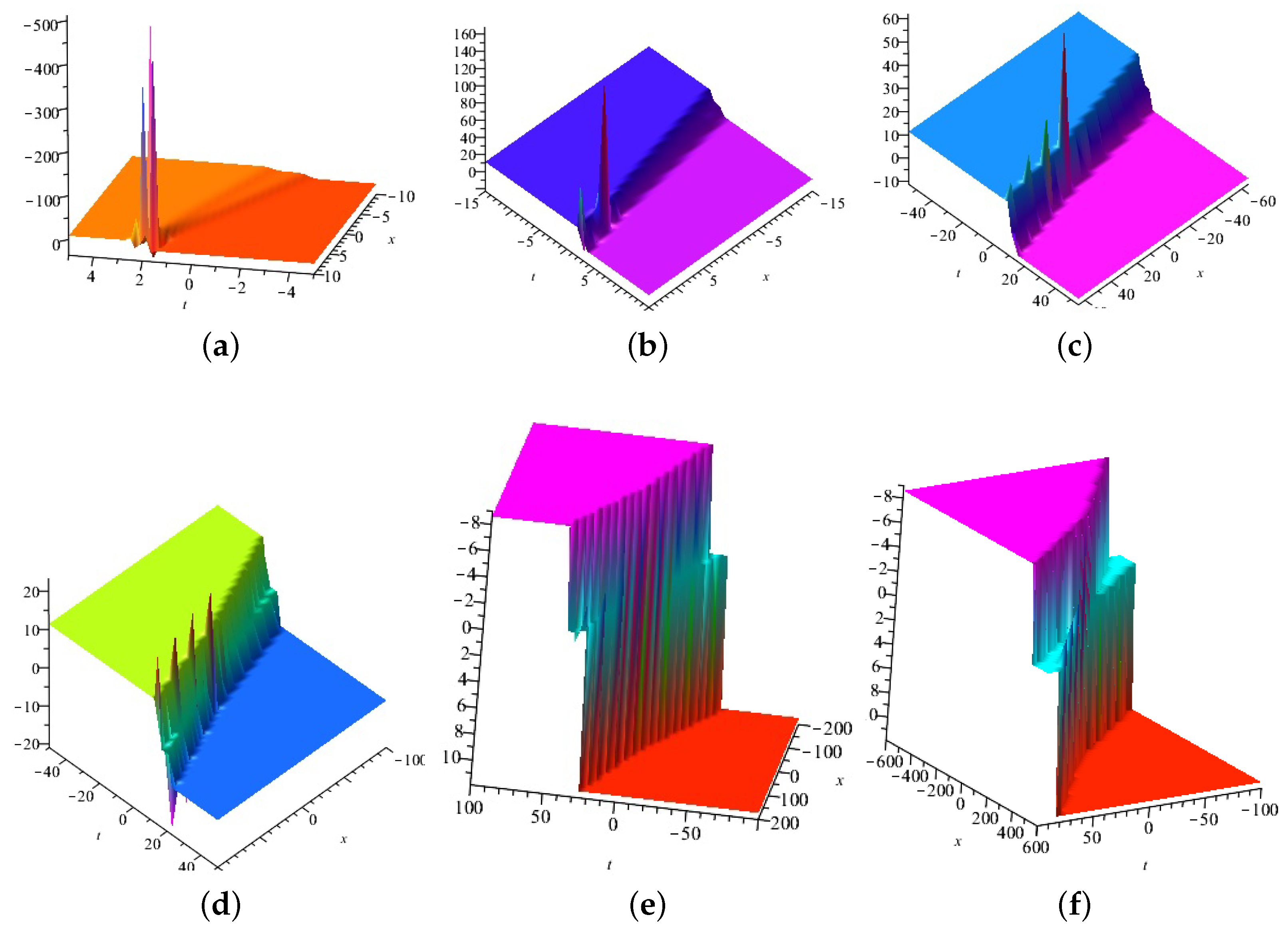
3.3. Mathematical Analysis of the MEFM for (61)

In this Subsection, we use the MEFM to obtain novel solutions for (61).
  • One wave solutions for (61):
In a similar way, we have
P 1 = P 0 Q 1 Q 0 , S 1 : arbitrary , w 1 : arbitrary .
With the above values, we have
u ( x , t ) = P 0 + P 0 Q 1 Q 0 Ξ 1 Q 0 + Q 1 Ξ 1 .
where Ξ 1 is defined in (65).
  • Two wave solutions for (61):
In a similar way, we have
P 12 : arbitrary , ω 1 = 3 S 1 + 3 R 1 , ω 2 = 3 S 2 + 3 R 2 .
With the above values, we have
u ( x , t ) = 2 ( S 1 Ξ 1 + S 2 Ξ 2 + P 12 ( S 1 + S 2 ) Ξ 1 Ξ 2 ) 1 + Ξ 1 + Ξ 2 + P 12 Ξ 1 Ξ 2 .
where Ξ i is defined in (45).
  • Three wave solutions for (61):
In a similar way, we have
P 12 = arbitrary , P 13 = arbitrary , P 23 : 0 ω 1 = 3 S 1 + 3 R 1 , ω 2 = 3 S 2 + 3 R 2 , ω 3 = 3 S 3 + 3 R 3 , R 1 = arbitrary , R 2 = arbitrary , R 3 = arbitrary , S 1 = arbitrary , S 2 = arbitrary , S 3 = arbitrary .
With the above values, we have
u ( x , t ) = [ 2 ( S 1 Ξ 1 + S 2 Ξ 2 + S 3 Ξ 3 + P 12 ( S 1 + S 2 ) Ξ 1 Ξ 2 + P 13 ( S 1 + S 3 ) Ξ 1 Ξ 3 ) ] / 1 + Ξ 1 + Ξ 2 + Ξ 3 + P 12 Ξ 1 Ξ 2 + P 13 Ξ 1 Ξ 3 ,
where Ξ i defined in (54).

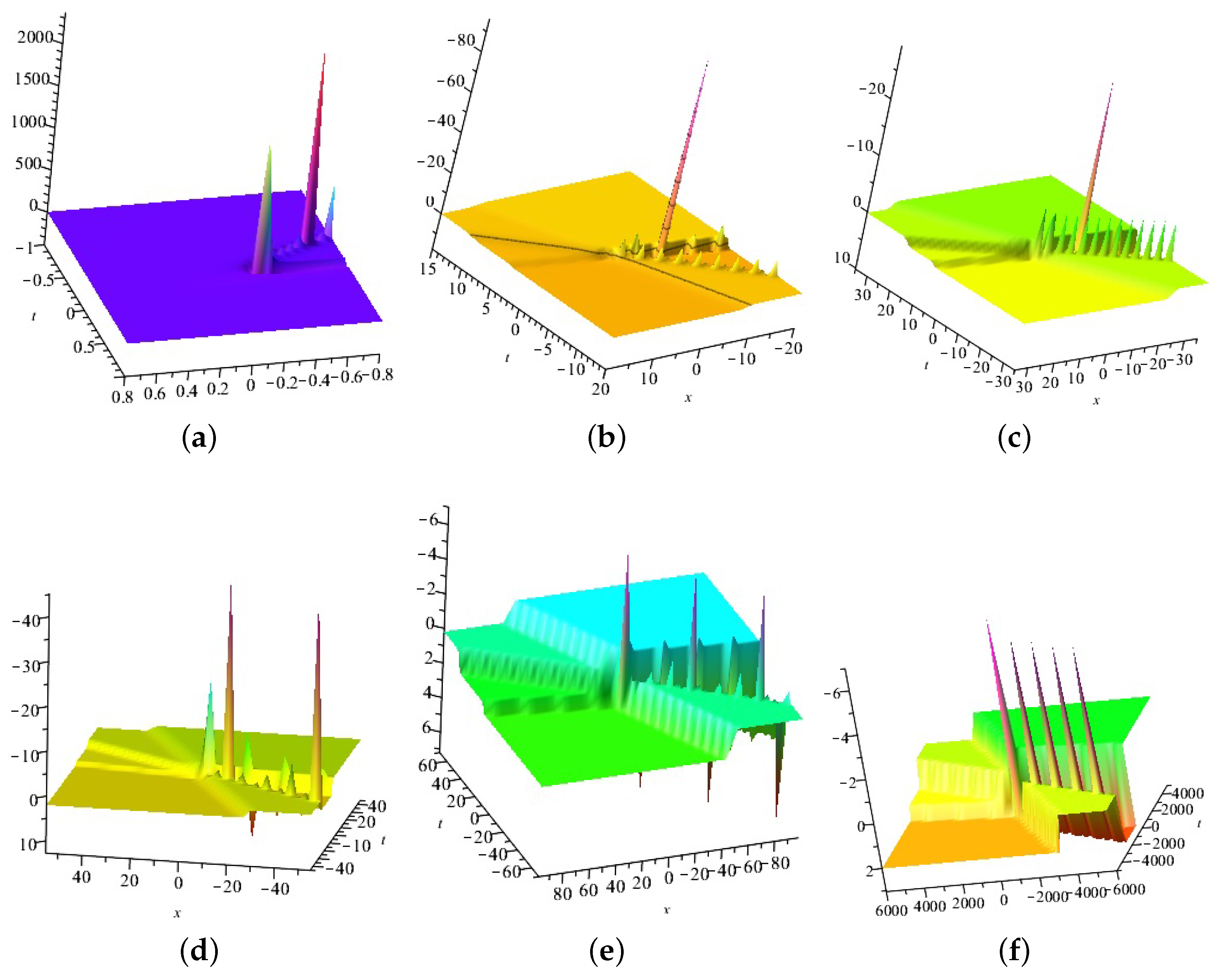
3.4. Mathematical Analysis of the MHTM for (61)

In this Subsection, we use the MHTM to obtain novel analytical solutions for the (2+1)-dimensional NPDE given by (61).
  • One wave solutions for (61):
Consider Ξ 1 = Ξ 1 ( x , y , t ) as
Ξ 1 = ϖ 1 tanh ( S 1 x + R 1 y ω 1 t ) ,
where ϖ 1 , S 1 , R 1 , and ω 1 are fixed. Therefore, we assume
K ( Ξ 1 ) = P 0 + P 1 Ξ 1 ,
H ( Ξ 1 ) = Q 0 + Q 1 Ξ 1 ,
where P 0 , P 1 , Q 0 , and Q 1 are fixed to be determined from (38). Thus, we obtain
u ( x , t ) = K ( Ξ 1 ) H ( Ξ 1 ) = P 0 + P 1 Ξ 1 Q 0 + Q 1 Ξ 1 .
By setting (68) into (61) and solving the system of linear equations, we have:
P 1 = Q 1 P 0 Q 0 , ω 1 : arbitrary .
Thus, we obtain
u ( x , t ) = P 0 + Q 1 P 0 Q 0 tanh ( S 1 x + R 1 y ω 1 t ) Q 0 + Q 1 tanh ( S 1 x + R 1 y ω 1 t ) .
Equation (69) is displayed in Figure 16 for S 1 = 0.90 , R 1 = 0.90 , Q 1 = 0.70 , Q 0 = 0.40 , P 0 = 0.90 , ω 1 = 0.5 , in diverse domains.
  • Two wave solutions for (61):
Consider Ξ i = Ξ i ( x , y , t ) , i = 1 , 2 , as
Ξ i = ϖ i tanh ( S i x + R i y ω i t ) , i = 1 , 2
where S i , ω i ,   ϖ i , and R i , are fixed. Therefore, we assume
K ( Ξ 1 , Ξ 2 ) = 2 ( S 1 Ξ 1 + S 2 Ξ 2 + P 12 ( S 1 + S 2 ) Ξ 1 Ξ 2 ) ,
H ( Ξ 1 , Ξ 2 ) = 1 + Ξ 1 + Ξ 2 + P 12 Ξ 1 Ξ 2 ,
where P 12 is a constant to be determined from (38). Therefore, we have
u ( x , t ) = 2 ( S 1 Ξ 1 + S 2 Ξ 2 + P 12 ( S 1 + S 2 ) Ξ 1 Ξ 2 ) 1 + Ξ 1 + Ξ 2 + P 12 Ξ 1 Ξ 2 .
By setting (73) into (61), we have:
P 12 : arbitrary , ω 1 = 3 S 1 + 3 R 1 , ω 2 = 3 S 2 + 3 R 2 .
By inserting the above values in (49), we obtain
u ( x , t ) = 2 ( S 1 Ξ 1 + S 2 Ξ 2 + P 12 ( S 1 + S 2 ) Ξ 1 Ξ 2 ) 1 + Ξ 1 + Ξ 2 + P 12 Ξ 1 Ξ 2 .
where Ξ i is defined in (70).
The Equation (74) is displayed in Figure 17 with values R 1 : = 0.80 , R 2 = 0.50 , S 1 = 0.60 , S 2 = 0.9 , P 12 = 0.70 , in different domains.
  • Three wave solutions for (61):
Consider Ξ i = Ξ i ( x , y , t ) , i = 1 , 2 , 3 , as
Ξ i = ϖ i tanh ( S i x + R i y ω i t ) , i = 1 , 2 , 3
in which ω i , S i ,   ϖ i , and R i , are fixed. Therefore, we assume
K ( Ξ 1 , Ξ 2 , Ξ 3 ) = 2 ( S 1 Ξ 1 + S 2 Ξ 2 + S 3 Ξ 3 + P 12 ( S 1 + S 2 ) Ξ 1 Ξ 2 + P 13 ( S 1 + S 3 ) Ξ 1 Ξ 3 + P 23 ( S 2 + S 3 ) Ξ 2 Ξ 3 + P 12 P 13 P 23 ( S 1 + S 2 + S 3 ) Ξ 1 Ξ 2 Ξ 3 ) ,
and
H ( Ξ 1 , Ξ 2 , Ξ 3 ) = 1 + Ξ 1 + Ξ 2 + Ξ 3 + P 12 Ξ 1 Ξ 2 + P 13 Ξ 1 Ξ 3 + P 23 Ξ 2 Ξ 3 + P 12 P 13 P 23 Ξ 1 Ξ 2 Ξ 3 ,
where P 12 , P 13 , and P 23 are fixed to be specified from (61). Thus, we obtain
u ( x , t ) = [ 2 ( S 1 Ξ 1 + S 2 Ξ 2 + S 3 Ξ 3 + P 12 ( S 1 + S 2 ) Ξ 1 Ξ 2 + P 13 ( S 1 + S 3 ) Ξ 1 Ξ 3 + P 23 ( S 2 + S 3 ) Ξ 2 Ξ 3 + P 12 P 13 P 23 ( S 1 + S 2 + S 3 ) Ξ 1 Ξ 2 Ξ 3 ) ] / 1 + Ξ 1 + Ξ 2 + Ξ 3 + P 12 Ξ 1 Ξ 2 + P 13 Ξ 1 Ξ 3 + P 23 Ξ 2 Ξ 3 + P 12 P 13 P 23 Ξ 1 Ξ 2 Ξ 3 .
By setting (76) into (61), we obtain:
P 12 = arbitrary , P 13 = arbitrary , P 23 : 0 ω 1 = 3 S 1 + 3 R 1 , ω 2 = 3 S 2 + 3 R 2 , ω 3 = 3 S 3 + 3 R 3 , R 1 = arbitrary , R 2 = arbitrary , R 3 = arbitrary , S 1 = arbitrary , S 2 = arbitrary , S 3 = arbitrary .
Therefore, we obtain
u ( x , t ) = [ 2 ( S 1 Ξ 1 + S 2 Ξ 2 + S 3 Ξ 3 + P 12 ( S 1 + S 2 ) Ξ 1 Ξ 2 + P 13 ( S 1 + S 3 ) Ξ 1 Ξ 3 ) ] / 1 + Ξ 1 + Ξ 2 + Ξ 3 + P 12 Ξ 1 Ξ 2 + P 13 Ξ 1 Ξ 3 .
where Ξ i is defined in (75).
Equation (77) is displayed in Figure 18, with values P 13 = 0.50 , P 12 = 3.50 , S 1 = 0.60 , S 2 = 0.50 , S 3 = 0.90 , R 1 = 0.20 , R 2 = 0.90 , R 3 = 0.70 , ω 3 = 0.50 , in diverse domains.

3.5. Discussion

We now compare the MEFM and the MHTM for NPDE (61). First, we examine the one wave solution for both methods. In this case, we obtain the following similar results for the two mentioned methods:
P 1 = Q 1 P 0 Q 0 , ω 1 : arbitrary .
Now, we consider the following solutions:
5 35 2 exp ( 0.8 x + 0.3 y 0.9 t ) 0.2 0.7 exp ( 0.8 x + 0.3 y 0.9 t ) ,
and
5 35 2 tanh ( 0.8 x + 0.3 y 0.9 t ) 0.2 0.7 tanh ( 0.8 x + 0.3 y 0.9 t ) .
In Figure 19, the (a), (b), (c) display the 2D with the diagrams of Equation (79) and the (d), (e), and (f) display the 2D with the diagrams of Equation (78) and also, the (g), (h), (f) display the 2D with the diagrams of differences between the (a), (d), (b), (e), and (c), (f). According to the (g), (h), (f), the differences obtained between the two methods is minor. But as you can see, the MEFM has a more accurate behavior than the MHTM. Figure 20 displays the 2D with the contour plots of Equations (78) and (79) and confirm the recent claim.
Next, we examine the two wave solution for both methods. In this case, we obtain the following similar results for the two mentioned methods:
P 12 : arbitrary , ω 1 = 3 S 1 + 3 R 1 , ω 2 = 3 S 2 + 3 R 2 .
Now, we consider the following solutions:
[ 2 ( S 1 Ξ 1 + S 2 Ξ 2 + P 12 ( S 1 + S 2 ) Ξ 1 Ξ 2 ) ] / [ 2 ( S 1 Ξ 1 + S 2 Ξ 2 + P 12 ( S 1 + S 2 ) Ξ 1 Ξ 2 ) ]
where
Ξ i = ϖ i exp ( S i x + R i y ω i t ) , i = 1 , 2
and
[ 2 ( S 1 Ξ 1 + S 2 Ξ 2 + P 12 ( S 1 + S 2 ) Ξ 1 Ξ 2 ) ] / [ 2 ( S 1 Ξ 1 + S 2 Ξ 2 + P 12 ( S 1 + S 2 ) Ξ 1 Ξ 2 ) ]
where
Ξ i = ϖ i tanh ( S i x + R i y ω i t ) , i = 1 , 2 .
Here, we set S 1 = 0.6 , S 2 = 0.9 , R 1 = 0.8 , R 2 = 0.5 and P 12 = 0.7 . Now, in Figure 21, the (e),(f),(g) display the 3D with the diagrams of Equation (80) and the (a),(b),(c) display the 3D with the diagrams of Equation (81). In Figure 22, the (d),(e),(f) display the contour plots of (80) and the (a),(b),(c) display the contour plots of Equation (81). We can observe that the results gained by the MEFM have higher accuracy than those of the MHTM. Also, the MEFM has a smoother behavior than the MHTM.
Now, we examine the three wave solution for both methods. In this case, we obtain the following similar results for the two mentioned methods:
P 12 = arbitrary , P 13 = arbitrary , P 23 : 0 ω 1 = 3 S 1 + 3 R 1 , ω 2 = 3 S 2 + 3 R 2 , ω 3 = 3 S 3 + 3 R 3 , R 1 = arbitrary , R 2 = arbitrary , R 3 = arbitrary , S 1 = arbitrary , S 2 = arbitrary , S 3 = arbitrary .
With the above values, we have
u ( x , t ) = [ 2 ( S 1 Ξ 1 + S 2 Ξ 2 + S 3 Ξ 3 + P 12 ( S 1 + S 2 ) Ξ 1 Ξ 2 + P 13 ( S 1 + S 3 ) Ξ 1 Ξ 3 ) ] / 1 + Ξ 1 + Ξ 2 + Ξ 3 + P 12 Ξ 1 Ξ 2 + P 13 Ξ 1 Ξ 3 ,
where
Ξ i = ϖ i exp ( S i x + R i y ω i t ) , i = 1 , 2 , 3
and
u ( x , t ) = [ 2 ( S 1 Ξ 1 + S 2 Ξ 2 + S 3 Ξ 3 + P 12 ( S 1 + S 2 ) Ξ 1 Ξ 2 + P 13 ( S 1 + S 3 ) Ξ 1 Ξ 3 ) ] / 1 + Ξ 1 + Ξ 2 + Ξ 3 + P 12 Ξ 1 Ξ 2 + P 13 Ξ 1 Ξ 3 ,
where
Ξ i = ϖ i tanh ( S i x + R i y ω i t ) , i = 1 , 2 , 3 .
Here, we set S 1 = 0.6 , S 2 = 0.5 , S 3 = 0.9 , R 1 = 0.2 , R 2 = 0.9 , R 3 = 0.7 and P 13 = 0.5 , P 12 = 1.5 . Now, in Figure 23, the (e), (f), (g) display the 3D with the diagrams of Equation (82) and (a), (b), (c) display the 3D with the diagrams of Equation (83). In Figure 24, the (g), (e), (f) display the contour plots of Equation (82) and the (a), (b), (c) display the contour plots of Equation (83). As you can observe, the MEFM provides more accurate and detailed results.
Now, according to Figure 19, Figure 20, Figure 21, Figure 22, Figure 23 and Figure 24, we can conclude that the MEFM provides a better description of NPDEs in specific domains. In addition, the numerical results of Equations (78)–(83) are displayed in Table 1, and they confirm the recent claims.
According to the Table 1, we calculate the differences between obtained solutions for fixed t , y and different values of x , in Table 2. As you can observe, the range of these differences obtained by MEFM changes between 0 and 0.003 for one-wave solutions. And for MHTM, these changes are between 0.04 and 0.07. This means that in MEFM, with small changes in the input, it causes small changes in the output and therefore we can conclude in this situation that this method shows more stable behavior than MHTM. In the same way, we have similar results for the three wave solutions.

4. Conclusions

In this present study, to solve the nonlinear PDEs that contain some high nonlinear terms, several relatively novel analytical techniques entitled the “exp function method (EFM)”, “multi-exp function method (MEFM)”, and “multi hyperbolic tangent method (MHTM)” are applied, analyzed and compared to each other. In our situation we showed that MEFM is a better method in comparison with the two other methods. The presented methods have many merits and advantages. Calculations in the govering methods are simple and straightforward. The reliability of the methods and the reduction in the size of computation give these methods a wider applicability and the results show that the MEFM is a powerful mathematical tool for solving systems of nonlinear partial differential equations. Indeed, the MEFM is motivated because it is easy to use and also because of the capability of computer algebra systems and the method provides a direct and systematic solution procedure that generalizes Hirota’s perturbation scheme. With the help of Maple, applying the approach to the NPDEs yield exact explicit one-wave, two-wave and three-wave solutions, which include one-soliton, two-soliton and three-soliton-type solutions.

Author Contributions

D.O. methodology, writing—original draft preparation. S.R.A. methodology, writing–original draft preparation. R.S. supervision and project administration. T.A. editing and methodology. All authors conceived of the study, participated in its design and coordination, drafted the manuscript, participated in the sequence alignment. All authors have read and agreed to the published version of the manuscript.

Funding

This research received no external funding.

Data Availability Statement

Here by we confirm that there is no available and applicable data for this research. The research process is independent from any dataset.

Conflicts of Interest

The authors declare no potential conflict of interests.

References

  1. Aderyani, S.R.; Saadati, R.; Vahidi, J.; Allahviranloo, T. The exact solutions of the conformable time-fractional modified nonlinear Schrödinger equation by the Trial equation method and modified Trial equation method. Adv. Math. Phys. 2022, 2022, 4318192. [Google Scholar] [CrossRef]
  2. Aderyani, S.R.; Saadati, R.; Vahidi, J.; Mlaiki, N.; Abdeljawad, T. The exact solutions of conformable time-fractional modified nonlinear Schrödinger equation by Direct algebraic method and Sine-Gordon expansion method. AIMS Math. 2022, 7, 10807–10827. [Google Scholar] [CrossRef]
  3. Aderyani, S.R.; Saadati, R.; Vahidi, J.; Gómez-Aguilar, J.F. The exact solutions of conformable time-fractional modified nonlinear Schrödinger equation by first integral method and functional variable method. Opt. Quantum Electron. 2022, 54, 218. [Google Scholar] [CrossRef]
  4. Aderyani, S.R.; Saadati, R.; O’Regan, D.; Inc, M. Soliton Solutions of the Nonlinear Time Fractional Harry Dym Equation in the Caputo Sense and the Symmetric Regularized Long Wave Equation in the Conformable Sense. Res. Sq. 2023. [Google Scholar] [CrossRef]
  5. Aderyani, S.R.; Saadati, R.; O’Regan, D.; Alshammari, F.S. Describing Water Wave Propagation Using the G G 2 –Expansion Method. Mathematics 2022, 11, 191. [Google Scholar] [CrossRef]
  6. Mirzazadeh, M.; Sharif, A.; Hashemi, M.S.; Akgül, A.; El Din, S.M. Optical solitons with an extended (3 + 1)-dimensional nonlinear conformable Schrödinger equation including cubic–quintic nonlinearity. Results Phys. 2023, 49, 106521. [Google Scholar] [CrossRef]
  7. Chu, Y.M.; Inc, M.; Hashemi, M.S.; Eshaghi, S. Analytical treatment of regularized Prabhakar fractional differential equations by invariant subspaces. Comput. Appl. Math. 2022, 41, 271. [Google Scholar] [CrossRef]
  8. Malik, S.; Hashemi, M.S.; Kumar, S.; Rezazadeh, H.; Mahmoud, W.; Osman, M.S. Application of new Kudryashov method to various nonlinear partial differential equations. Opt. Quantum Electron. 2023, 55, 8. [Google Scholar] [CrossRef]
  9. Xie, X.; Wang, T.; Zhang, W. Existence of solutions for the (p, q)-Laplacian equation with nonlocal Choquard reaction. Appl. Math. Lett. 2023, 135, 108418. [Google Scholar] [CrossRef]
  10. Qin, X.; Liu, Z.; Liu, Y.; Liu, S.; Yang, B.; Yin, L.; Liu, M.; Zheng, W. User OCEAN personality model construction method using a BP neural network. Electronics 2022, 11, 3022. [Google Scholar] [CrossRef]
  11. Liu, M.; Gu, Q.; Yang, B.; Yin, Z.; Liu, S.; Yin, L.; Zheng, W. Kinematics Model Optimization Algorithm for Six Degrees of Freedom Parallel Platform. Appl. Sci. 2023, 13, 3082. [Google Scholar] [CrossRef]
  12. Ye, R.; Liu, P.; Shi, K.; Yan, B. State damping control: A novel simple method of rotor UAV with high performance. IEEE Access 2020, 8, 214346–214357. [Google Scholar] [CrossRef]
  13. Madina, B.; Gumilyov, L.N. Determination of the most effective location of environmental hardenings in concrete cooling tower under far-source seismic using linear spectral dynamic analysis results. J. Res. Sci. Eng. Technol. 2020, 8, 22–24. [Google Scholar] [CrossRef]
  14. Aslanova, F. A comparative study of the hardness and force analysis methods used in truss optimization with metaheuristic algorithms and under dynamic loading. Journal of Research in Science. Eng. Technol. 2020, 8, 25–33. [Google Scholar] [CrossRef]
  15. Muhamad, K.A.; Tanriverdi, T.; Mahmud, A.A.; Baskonus, H.M. Interaction Characteristics of the Riemann Wave Propagation in the (2 + 1)-Dimensional Generalized Breaking Soliton System. Int. J. Comput. Math. 2023, 100, 1340–1355. [Google Scholar] [CrossRef]
  16. He, J.H.; Wu, X.H. Exp-function method for nonlinear wave equations. Chaos Solitons Fractals 2006, 30, 700–708. [Google Scholar] [CrossRef]
  17. Rezazadeh, H.; Zabihi, A.; Davodi, A.G.; Ansari, R.; Ahmad, H.; Yao, S.W. New optical solitons of double Sine-Gordon equation using exact solutions methods. Results Phys. 2023, 49, 106452. [Google Scholar] [CrossRef]
  18. Guo, T.; Zaky, M.A.; Hendy, A.S.; Qiu, W. Pointwise error analysis of the BDF3 compact finite difference scheme for viscous Burgers’ equations. Appl. Numer. Math. 2023, 185, 260–277. [Google Scholar] [CrossRef]
  19. Yiasir Arafat, S.M.; Fatema, K.; Rayhanul Islam, S.M.; Islam, M.E.; Ali Akbar, M.; Osman, M.S. The mathematical and wave profile analysis of the Maccari system in nonlinear physical phenomena. Opt. Quantum Electron. 2023, 55, 136. [Google Scholar] [CrossRef]
  20. Wang, K. New fractal soliton solutions for the coupled fractional Klein-Gordon equation with β-fractional derivative. Fractals 2023, 31, 2350003. [Google Scholar] [CrossRef]
  21. Vivas-Cortez, M.; Akram, G.; Sadaf, M.; Arshed, S.; Rehan, K.; Farooq, K. Traveling wave behavior of new (2+1)-dimensional combined KdV–mKdV equation. Results Phys. 2023, 45, 106244. [Google Scholar] [CrossRef]
  22. Yao, S.W.; Zafar, A.; Urooj, A.; Tariq, B.; Shakeel, M.; Inc, M. Novel solutions to the coupled KdV equations and the coupled system of variant Boussinesq equations. Results Phys. 2023, 45, 106249. [Google Scholar] [CrossRef]
  23. Shakir, A.P.; Sulaiman, T.A.; Ismael, H.F.; Shah, N.A.; Eldin, S.M. Multiple fusion solutions and other waves behavior to the Broer-Kaup-Kupershmidt system. Alex. Eng. J. 2023, 74, 559–567. [Google Scholar] [CrossRef]
  24. Cheng, C.D.; Tian, B.; Zhou, T.Y.; Shen, Y. Wronskian solutions and Pfaffianization for a (3+1)-dimensional generalized variable-coefficient Kadomtsev-Petviashvili equation in a fluid or plasma. Phys. Fluids 2023, 35, 037101. [Google Scholar] [CrossRef]
  25. Shakeel, M.; Shah, N.A.; Chung, J.D. Modified Exp-Function Method to Find Exact Solutions of Microtubules Nonlinear Dynamics Models. Symmetry 2023, 15, 360. [Google Scholar] [CrossRef]
  26. Shakeel, M.; Alaoui, M.K.; Zidan, A.M.; Shah, N.A. Closed form solutions for the generalized fifth-order KDV equation by using the modified exp-function method. J. Ocean. Eng. Sci. 2022, in press. [Google Scholar] [CrossRef]
  27. Zulfiqar, A.; Ahmad, J.; Ul-Hassan, Q.M. Analysis of some new wave solutions of fractional order generalized Pochhammer-chree equation using exp-function method. Opt. Quantum Electron. 2022, 54, 735. [Google Scholar] [CrossRef]
  28. Pan, X.J.; Dai, C.Q. Explicit solutions of a generalized wick-type stochastic Korteveg–de Vries equation. Phys. Scr. 2009, 80, 065006. [Google Scholar] [CrossRef]
  29. Zhang, S. Exp-function method: Solitary, periodic and rational wave solutions of nonlinear evolution equations. Nonlinear Sci. Lett. A 2010, 2, 143–146. [Google Scholar]
  30. Ma, W.X.; Huang, T.; Zhang, Y. A multiple exp-function method for nonlinear differential equations and its application. Phys. Scr. 2010, 82, 065003. [Google Scholar] [CrossRef]
  31. Yajima, N. Application of Hirota’s Method to a Perturbed System. J. Phys. Soc. Jpn. 1982, 51, 1298–1302. [Google Scholar] [CrossRef]
  32. Gilson, C.; Pickering, A. Factorization and Painlevé analysis of a class of nonlinear third-order partial differential equations. J. Phys. A Math. Gen. 1995, 28, 2871. [Google Scholar] [CrossRef]
  33. Whitham, G.B. Linear and Nonlinear Waves; John Wiley and Sons: Hoboken, NJ, USA, 2011. [Google Scholar]
  34. Camassa, R.; Holm, D.D. An integrable shallow water equation with peaked solitons. Phys. Rev. Lett. 1993, 71, 1661. [Google Scholar] [CrossRef]
  35. Irshad, A.; Mohyud, S.T. Tanh-Coth Method for Nonlinear Differential Equations. Stud. Nonlinear Sci. 2012, 3, 24–48. [Google Scholar]
  36. Fan, X.; Yang, S.; Zhao, D. Travelling wave solutions for the Gilson-Pickering equation by using the simplified G/G-expansion method. Int. J. Nonlinear Sci. 2009, 8, 368–373. [Google Scholar]
  37. Chen, A.; Huang, W.; Tang, S. Bifurcations of travelling wave solutions for the Gilson–Pickering equation. Nonlinear Anal. Real World Appl. 2009, 10, 2659–2665. [Google Scholar] [CrossRef]
  38. Garshasbi, M.; Khakzad, M. The RBF collocation method of lines for the numerical solution of the CH- equation. J. Adv. Res. Dyn. Control Syst. 2015, 4, 65–83. [Google Scholar]
  39. Zabihi, F.; Saffarian, M. A not-a-knot meshless method with radial basis functions for numerical solutions of Gilson–Pickering equation. Eng. Comput. 2018, 34, 37–44. [Google Scholar] [CrossRef]
  40. Ali, K.K.; Mehanna, M.S. Traveling wave solutions and numerical solutions of Gilson–Pickering equation. Results Phys. 2021, 28, 104596. [Google Scholar] [CrossRef]
  41. Bilal, M.; Seadawy, A.R.; Younis, M.; Rizvi, S.T.R.; El-Rashidy, K.; Mahmoud, S.F. Analytical wave structures in plasma physics modelled by Gilson-Pickering equation by two integration norms. Results Phys. 2021, 23, 103959. [Google Scholar] [CrossRef]
  42. Ali, K.K.; Dutta, H.; Yilmazer, R.; Noeiaghdam, S. On the new wave behaviors of the Gilson-Pickering equation. Front. Phys. 2020, 8, 54. [Google Scholar] [CrossRef]
  43. Yokuş, A.; Durur, H.; Abro, K.A.; Kaya, D. Role of Gilson–Pickering equation for the different types of soliton solutions: A nonlinear analysis. Eur. Phys. J. Plus 2020, 135, 1–19. [Google Scholar] [CrossRef]
  44. Rezazadeh, H.; Jhangeer, A.; Tala-Tebue, E.; Hashemi, M.S.; Sharif, S.; Ahmad, H.; Yao, S.W. New wave surfaces and bifurcation of nonlinear periodic waves for Gilson-Pickering equation. Results Phys. 2021, 24, 104192. [Google Scholar] [CrossRef]
  45. Samir, I.; Badra, N.; Ahmed, H.M.; Arnous, A.H.; Ghanem, A.S. Solitary wave solutions and other solutions for Gilson–Pickering equation by using the modified extended mapping method. Results Phys. 2022, 36, 105427. [Google Scholar] [CrossRef]
  46. Hu, X.; Jin, Y.; Zhou, K. Optimal System and Group Invariant Solutions of the Whitham-Broer-Kaup System. Adv. Math. Phys. 2019, 2019, 1892481. [Google Scholar] [CrossRef]
  47. Abouelregal, A.E.; Akgöz, B.; Civalek, Ö. Magneto-thermoelastic interactions in an unbounded orthotropic viscoelastic solid under the Hall current effect by the fourth-order Moore-Gibson-Thompson equation. Comput. Math. Appl. 2023, 141, 102–115. [Google Scholar] [CrossRef]
  48. Abouelregal, A.E.; Ersoy, H.; Civalek, Ö. Solution of Moore-Gibson-Thompson equation of an unbounded medium with a cylindrical hole. Mathematics 2021, 9, 1536. [Google Scholar] [CrossRef]
  49. Aderyani, S.R.; Saadati, R.; Vahidi, J. Multiple exp-function method to solve the nonlinear space–time fractional partial differential symmetric regularized long wave (SRLW) equation and the (1 + 1)-dimensional Benjamin–Ono equation. Int. J. Mod. Phys. B 2022, 37, 2350213. [Google Scholar] [CrossRef]
  50. Aderyani, S.R.; Saadati, R.; O’Regan, D.; Alshammari, F.S. Existence, Uniqueness and Stability Analysis with the Multiple Exp Function Method for NPDEs. Mathematics 2022, 10, 4151. [Google Scholar] [CrossRef]
  51. Lai, S.; Luo, K. Wave breaking to a shallow water wave equation involving the Fornberg-Whitham model. J. Differ. Equ. 2023, 344, 509–521. [Google Scholar] [CrossRef]
  52. Boutarfa, B.; Akgül, A.; Inc, M. New approach for the Fornberg–Whitham type equations. J. Comput. Appl. Math. 2017, 312, 13–26. [Google Scholar] [CrossRef]
  53. Yu, Z.; Shi, X.; Qiu, X.; Zhou, J.; Chen, X.; Gou, Y. Optimization of postblast ore boundary determination using a novel sine cosine algorithm-based random forest technique and Monte Carlo simulation. Eng. Optim. 2021, 53, 1467–1482. [Google Scholar] [CrossRef]
  54. Polyanin, A.D.; Zaitsev, V.F. Handbook of Nonlinear Partial Differential Equations; Chapman and Hall/CRC: Boca Raton, FL, USA, 2016. [Google Scholar]
Figure 1. The 3D and 2D with the plots of Equation (18), for α = 0.5 , b 0 = 5 , b 1 = 4.5 . (a) 3D with the plots of Equation (18), for α = 0.5 , b 0 = 5 b 1 = 4.5 . (b) 2D with the plots of Equation (18), for α = 0.5 , b 0 = 5 .
Axioms 13 00074 g001
Figure 2. The 3D and 2D with the plots of Equation (26), for α = 0.5 , a 2 = 2.5 , b 2 = 3.5 , b 2 = 3 . (a) The 3D with the plot of Equation (26). (b) The 2D with the plot of Equation (26).
Axioms 13 00074 g002
Figure 3. The 3D and 2D with the plots of Equation (27), for α = 0.5 , a 2 = 3 , b 2 = 3.5 , b 0 = 5 . (a) The 3D with the plot of Equation (27). (b) The 2D with the plot of Equation (27).
Axioms 13 00074 g003
Figure 4. The 3D, 2D and the contour plots for (44). (a) The 3D plot for (44). (b) The 2D plot for (44). (c) The contour plot for (44). (d) The contour plot for (44).
Axioms 13 00074 g004
Figure 5. The (ad) display the 3D, 2D and the contour plots for the real part of Equation (50).
Axioms 13 00074 g005
Figure 6. The (ad) display the 3D, 2D and the contour plots for the imaginary part of Equation (50).
Axioms 13 00074 g006
Figure 7. The (ad) display the 3D, 2D and the contour plots for the real part of Equation (51).
Axioms 13 00074 g007
Figure 8. The (ad) display the 3D, 2D and the contour plots for the imaginary part of Equation (51).
Axioms 13 00074 g008
Figure 9. The (ad) display the 3D, 2D and the contour plots for Equation (52).
Axioms 13 00074 g009
Figure 10. The (ad) display the 3D, 2D and the contour plots for Equation (53).
Axioms 13 00074 g010
Figure 11. The (ad) display the 3D, 2D and the contour plots for Equation (57).
Axioms 13 00074 g011
Figure 12. The (ad) display the 3D, 2D and the contour plots for Equation (58).
Axioms 13 00074 g012
Figure 13. The (ad) display the 3D, 2D and the contour plots for Equation (59).
Axioms 13 00074 g013
Figure 14. The (ad) display the 3D, 2D and the contour plots for Equation (60).
Axioms 13 00074 g014
Figure 15. The (ad) display the 3D, 2D and the contour plots for Equation (60).
Axioms 13 00074 g015
Figure 16. The (af) display the 3D with the plots of Equation (69) in different domains. And the (gi) display the contour plots for Equation (69) in different domains.
Axioms 13 00074 g016
Figure 17. The (af) display the 3D with the plots of Equation (74) in different domains.
Axioms 13 00074 g017
Figure 18. The (af) display the 3D with the plots of Equation (77) in different domains.
Axioms 13 00074 g018
Figure 19. The (ac) display the 2D with the diagrams of Equation (79) and the (df) display the 2D with the diagrams of Equation (78) and also, the (gi) display the 2D with the diagrams of differences between the (a,d), the (b,e), and the (c,f).
Axioms 13 00074 g019
Figure 20. The (ac) display the 2D with the contour plots of Equation (79) and the (df) display the 2D with the contour plots of Equation (78).
Axioms 13 00074 g020
Figure 21. The (df) display the 3D with the diagrams of (80) and the (ac) display the 3D with the diagrams of (81).
Axioms 13 00074 g021
Figure 22. The (df) display the contour plots of Equation (80) and the (ac) display the contour plots of Equation (81).
Axioms 13 00074 g022
Figure 23. The (df) display the 3D with the diagrams of Equation (82) and (ac) display the 3D with the diagrams of Equation (83).
Axioms 13 00074 g023
Figure 24. The (df) display the contour plots of Equation (82) and the (ac) display the contour plots of Equation (83).
Axioms 13 00074 g024
Table 1. Numerical results of Equations (78)–(83).
One-Wave SolutionTwo-Wave SolutionThree-Wave Solution
y = t = 0.20x u MEFM u MHTM u MEFM u MHTM u MEFM u MHTM
0.2024.9999999925.000000000.175385190.949521150.182260020.02165664
0.3025.0000000225.000000000.177261730.870769050.184347950.03003873
0.4025.0000000125.000000010.179149240.799987660.186452540.03870608
0.5025.0000000024.999999990.181047540.736047040.188573760.04767017
0.6024.9999999925.000000000.181047540.678021340.190711540.05694300
0.7024.9999999925.000000000.184875830.625144650.192865840.06653706
0.8025.0000000125.000000010.186905430.576777950.195036580.07646545
0.9025.0000000025.000000000.188745100.532383840.197223700.08674179
Table 2. According to the Table 1, we calculate the differences between obtained solutions for fixed t , y and different values of x .
One-Wave SolutionTwo-Waves OlutionThree-Wave Solution
y = t = 0.20x Δ u MEFM Δ u MHTM Δ u MEFM Δ u MHTM Δ u MEFM Δ u MHTM
0.20–0.300.000000010.000000000.001876540.078752100.002087930.00838209
0.30–0.400.000000010.000000010.001887510.070781390.002104590.00866735
0.40–0.500.000000010.000000020.001809830.063940620.002121220.00896409
0.50–0.600.000000010.000000010.000000000.058025700.002137780.00927283
0.60–0.700.000000000.000000000.0033828290.052876690.002154300.00959406
0.70–0.800.000000010.000000010.002029600.048366700.002170740.00992839
0.80–0.900.000000010.000000000.001839670.044394110.002187120.01027634
Disclaimer/Publisher’s Note: The statements, opinions and data contained in all publications are solely those of the individual author(s) and contributor(s) and not of MDPI and/or the editor(s). MDPI and/or the editor(s) disclaim responsibility for any injury to people or property resulting from any ideas, methods, instructions or products referred to in the content.

