Abstract
In this work, an analogue to the Pauli spin matrices is presented and investigated. The proposed Hermitian spin matrices exhibit four symmetries for spin-1/n particles. The spin projection operators are derived, and the electrodynamics for hypothetical spin-1/2 fermions are explored using the proposed spin matrices. The fermionic quantum Heisenberg model is constructed using the proposed spin matrices, and comparative studies against simulation results using the Pauli spin matrices are conducted. Further analysis of the key findings as well as discussions on extending the proposed spin matrix framework to describe hypothetical bosonic systems (spin-1 particles) are provided.
Keywords:
exotic particle dynamics; novel Hermitian spin matrices; Pauli matrices; electrodynamics; fermionic quantum Heisenberg model; bosonic spin systems MSC:
81T05; 81T11; 81T32; 81-10
1. Introduction
In this work, four novel Hermitian spin matrices are introduced as analogues to the Pauli spin matrices. The proposed spin matrices exhibit the following symmetrical relations with their respective basis using the novel spin matrices for particles with spin 1/n, where n > 0:
where , and the complex conjugate relation . Four possible symmetrical relations with their respective basis are then ascertained using the proposed spin matrices for n > 0. Although the analysis in this work could be carried out with any of the symmetrical relations given in Equation (1), the scope of the present manuscript is limited to Relation I. Thus, this work aims to explore hypothetical fermion dynamics using the proposed Hermitian spin matrices for Relation I in Equation (1) at n = 2.
Identifying and characterizing novel Hermitian operators is of primary interest in mathematical and computational physics. An example of research in this direction is seen in Dita (2005) [1]. In that work, the authors proposed an explicit parameterization for arbitrary n-dimensional Hermitian matrices on the Hilbert space, . These operators were considered as density matrices or Hamiltonians for finite-level quantum systems, where they provide a complete solution to the parametrization of the problem. In Dita (2005) [1], an interesting result was discovered when the author obtained an alternative parametrization of the Stiefel and Grassmann manifolds using these parameterized Hermitian operators. Similarly, in Allard and Härd (2001) [2], a complete Hermitian operator basis was proposed for any arbitrary spin quantum number. The authors in that work proposed the basis for application in nuclear magnetic resonance simulations. In Allard and Härd (2001) [2], the key advantage of the proposed Hermitian operator basis is that it makes the quantum mechanical master equation (Liouville–von Neumann equation) real-valued. Therefore, the physical observables obtained are real-valued since the Hermitian operator has real eigenvalues (similar to this work).
Besides focusing on purely Hermitian operators, research in the past decade has also been carried out on the non-Hermitian formulation of quantum mechanics [3,4,5]. Non-Hermitian physics has found various applications in phenomena related to optics, photonics and condensed matter systems. In the recent work of Ju et al. (2022) [6], the authors proposed a formalism to transform non-Hermitian Hamiltonians to Hermitian ones without altering the underlying physics. Another interesting work is presented in Fring and Tenney (2021) [7]. In that work, the authors explored exactly solvable time-dependent non-Hermitian quantum systems. They employed complex point transformations for constructing non-Hermitian first integrals, metric operators and time-dependent Dyson maps for non-Hermitian quantum systems. A similar line of investigation is pursued by Koussa et al. (2018) [8], where the time evolution of quantum systems was analyzed with respect to the time-dependent non-Hermitian Hamiltonian. This non-Hermitian Hamiltonian exhibits SU(1,1) and SU(2) dynamical symmetry. In Koussa et al. (2018) [8], the exact solutions to the Schrödinger equations for both symmetries with respect to the eigenstates of the pseudo-Hermitian operators were obtained. In a study by Luiz et al. (2020) [9], the unitarity of time evolution and the observability of non-Hermitian Hamiltonians were explored in the context of time-dependent Dyson maps. The authors in that work derived the time-dependent Dyson map for two instances. The first was via a constructed Schrödinger-like equation, while the second instance was carried out using a non-Hermitian Hamiltonian.
An interesting review on the investigation of non-Hermitian dynamics in magnetic systems is presented in Hurst and Flebus (2022) [10]. In that work, the authors describe non-Hermitian frameworks in magnonic and hybrid magnonic systems—e.g., magnon-qubit coupling schemes and cavity magnonic systems. The mentioned review also discusses recent advances in the dynamics of inherently lossy magnetic systems as well as systems with gain induced by the external application of spin currents. In Zhang et al. (2021) [11], the authors theoretically investigate the critical phases in steady states of non-unitary free fermion dynamics. The authors of that work explored the physics of such critical phases by developing solvable static/Brownian quadratic Sachdev-Ye-Kitaev chains with non-Hermitian dynamics. Another interesting research review on non-Hermitian dynamics of open Markovian quantum systems is seen in the study by Roccati et al. (2022) [12]. In that review, the authors outline some critical developments in the last two decades in studies related to non-Hermitian Hamiltonians and their connections to the Gorini–Kossakowski–Sudarshan–Lindblad master equation. Besides non-Hermitian quantum dynamics, pseudo-Hermitian systems have also been the subject of recent investigations. For instance, in the work of Cius et al. (2022) [13], the authors analyzed the pseudo-Hermitian dynamical Casimir effect. The authors present a novel non-Hermitian version of the effective Law’s Hamiltonian to describe the mentioned effect. Another example of pseudo-Hermitian frameworks is seen in He et al. (2023) [14]. In that work, the authors explored the topology of a pseudo-Hermitian Chern insulator defined using the basis of q-deformed Pauli matrices (related to deformed algebras). The key finding of that work was obtained for a completely nonequilibrium case where the quantum evolution after quenching was dictated by a Floquet pseudo-Hermitian Hamiltonian. Similarly, in Fring and Taira (2020) [15] the authors employed a pseudo-Hermitian approach to Goldstone’s theorem in non-Abelian and non-Hermitian quantum field theories. In that work, a detailed analysis of a non-Hermitian field theory with two complex scalar fields (with two components) exhibiting SU(2) symmetry was presented. Zhu et al. (2021) [16] demonstrated that several two- and three-dimensional pseudo-Hermitian phases could be constructed using q-deformed matrices. In addition to investigations related to topological bulk states, quantum metrics and non-Abelian tensor Berry connections, an experimental protocol was proposed for the empirical validation (of the proposed models). The following works provide current developments on research efforts in the direction of non-Hermitian and pseudo-Hermitian frameworks: Okuma and Sato, (2023) [17], Ashida et al., (2020) [5], Kunst and Dwivedi (2019) [18] and Feinberg and Riser, (2021) [19].
This paper is organized as follows: The second and third sections describe the properties of the proposed spin matrices and their respective projection operators. In the fourth section, the electrodynamics of hypothetical fermions are explored using the proposed spin matrices as operators in the Schrödinger–Pauli and Dirac equations. The fifth section compares spin chain simulation results using the proposed spin matrices and the Pauli spin matrices. The sixth section provides further analysis of bosonic systems. This paper ends with the key conclusions from this research along with some ideas on directions for future research.
2. Analogue Spin Matrices
Pauli spin matrices serve as quantum operators corresponding to observables for the spin of fermions in each spatial direction: . In this work, four spin matrices are proposed as analogues to the Pauli spin matrices, (see Equation (1)). The proposed spin matrices, , are constructed from the Pauli matrices as follows:
For a particle with spin , the proposed Hermitian spin matrices follow the complex conjugate transpose relations:
The proposed matrices in Relation I exhibit the following symmetry:
where , = . In addition, the identity matrix is represented as follows:
The parameter, n > 0, is real-valued. If the parameter, n, is complex-valued, then the proposed matrices will lose their Hermitian properties. Similar to the Pauli matrices, the following matrix properties apply to arbitrary n:
However, unlike the Pauli matrices, the proposed matrices are not involutory. The following relationships exist between the proposed matrices: and . This introduces the possibility of simplifying the analysis of three-dimensional observables to two dimensions. The proposed matrices have the following commutative properties:
The commutation relations for the proposed matrices, where , are as follows:
On the other hand, the anti-commutation relations for the proposed matrices, where , are as follows:
The anti-commutator operation for the squared spin matrices, and , is as follows:
The vector properties of the proposed spin matrices are proved in the Appendix A. Using the proposed matrices, an analogue to the gamma matrices in the Dirac basis is then constructed for Relation I:
The proposed time-like gamma matrix is then as follows:
As with the Pauli matrices, all the proposed gamma matrices are Hermitian. Hence, these matrices yield real eigenvalues (real quantum energy states). The anticommutation relations for the proposed gamma matrices are as follows:
As with the conventional gamma matrices, the matrix properties for n = 2 are as follows:
3. Spin Projection Operators
In this section, the spin projection operators are obtained for the exotic fermions using the proposed spin matrices. A formulation for spin projection operators for fermions with spin- at n = 2 is provided. The two-component spinor is then employed to represent the quantum state of a fermion using the proposed spin matrices. The spin projection operator, S1, is expressed as follows:
where is the reduced Planck’s constant. The eigenvalues for S1 are and . The eigenvectors for S1 are and . The eigenspinor representations are then as follows:
The spin projection operator, S2, is expressed as follows:
The eigenvectors for S2 are and , and the eigenspinor representations are then as follows:
The spin projection operator, S3, is expressed as follows:
The eigenvectors for S3 are and , and the eigenspinor representations are then as follows:
An interesting difference with the Pauli spin projection operators is that for the operator S1, the spin state contains a small imaginary contribution of 3.92523 × 10⁻¹⁷i.
4. Electrodynamics
In this section, the non-relativistic electrodynamics of exotic fermions are explored using the Schrödinger–Pauli equation [20,21]. The Schrödinger–Pauli equation is presented using the proposed spin matrices at n = 2:
where m is the fermion mass, is the vector form of the momentum operator, is the magnetic vector potential, q is the fermion’s electric change, is the electric scalar potential, is the Hamiltonian (using the proposed spin matrices) and is the quantum state. The spin matrices are represented as the following vector: . By implementing the proposed spin matrices, the Schrödinger–Pauli equation yields solutions for the Hamiltonian, . Considering that the fermion (at n = 2) is subjected to a constant magnetic field within the Landau gauge [22],
where B is the uniform magnetic field. Solving the Schrödinger–Pauli equation for gives the following Hamiltonian operators:
This analysis is extended using the Landau symmetric gauge, where the magnetic vector potential is given as follows:
Solving the Schrödinger–Pauli equation within the Landau symmetric gauge using the spin matrix, , gives the following Hamiltonian operators:
In the context of relativistic quantum electrodynamics, the following Dirac equation is considered to determine the rest energy of the fermion placed in the electric potential, :
where m is the mass of the fermion, c is the speed of light and is the proposed gamma matrices. As with the conventional gamma matrices in the Dirac basis, it can be shown using Equation (25) that the rest energy of the hypothetical fermion at is equivalent to the energy of a particle placed in the electric potential, .
5. Simulation with Spin Chains
The proposed spin matrices are compared with the Pauli spin matrices by analyzing their respective behaviors in the context of a spin chain using the spin quantum Heisenberg model [23,24]. The one-dimensional Heisenberg model is utilized where magnetic interactions take place specifically between adjacent dipoles:
where J is the coupling constant, h is the external magnetic field, and the dipoles are described as the quantum operator acting on the Kronecker product of dimensions, 2N. Considering the coupling constant, , to be real-valued, the Hamiltonian operator is represented as follows:
where is the kth Pauli matrix on the jth lattice point with periodic boundary conditions. The Pauli matrices, , is defined as . In this work, the Heisenberg XXX model with is employed, where the coupling constants conform to the following equivalence: . The simulation is carried out using the Python programming language. To simplify the simulation, a qubit system is considered where the number of spins in the chain is limited to two. The following parameters are fixed in the simulation: coupling constant, J = 1 × 10⁻¹⁹ and B = 1 × 10⁻¹⁹ T. The simulation is performed at three temperature values: T1 = 10 K (low), T2 = 1000 K (medium), T4 = 10,000 K (high) and T4 = 100,000 K (very high). The spectrum of the Hamiltonian (i.e., energy states, , is then obtained for each spin state: . The configuration probability for each spin state, , is determined as follows:
where Z is the partition function and kB is the Boltzmann constant:
Computational experiments were performed by executing the simulation using Pauli matrices and the proposed spin matrices. The simulation routine for the spin chain used in this work is given in Algorithm 1:
| Algorithm 1: One-dimensional half-spin Heisenberg model |
START
|
Figure 1 provides the state probabilities generated from the simulations using the proposed spin matrices and Pauli matrices at different temperatures.
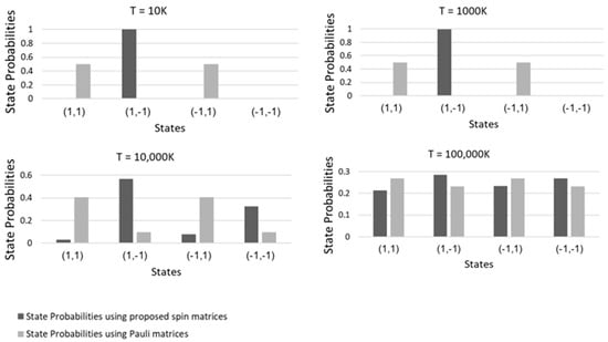
Figure 1.
State probabilities from simulations using the proposed spin matrices and Pauli matrices at different temperatures.
In Figure 1, the comparison of the state probabilities obtained using the proposed spin matrices and those generated using the proposed spin matrices for temperatures T = 100,000 K, 10,000 K, 1000 K and 10 K is shown. It can be observed that the overall dynamics of the system are similar to that of spin chains using Pauli matrices where the particles experience losses in magnetic spin orientation at higher temperatures, while the restoration of orientation rises at lower temperatures. To measure the difference between the state probabilities of the proposed matrices and the Pauli matrices, the Bures metric (or the Bures distance) is employed [25]. The Bures metric measures the statistical distance between two quantum states represented by their respective density matrices, . The Bures distance is measured as follows:
Figure 2 shows the Bures distance for the density states produced using the proposed matrices versus the Pauli matrices in the spin chain simulations using the Heisenberg spin model.
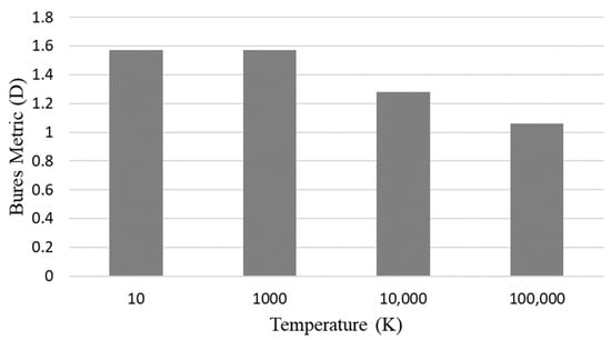
Figure 2.
Bures distance for the density states generated using the proposed matrices versus the Pauli matrices.
It can be seen in Figure 1 that at very high temperatures (T = 100,000 K), simulations undertaken using both sets of matrices generate similar state probabilities. At T = 100,000 K, the results show a somewhat equal distribution of probabilities among the four states. Despite this general similarity, the exact values of the state probabilities generated by the simulations using the Pauli matrices are distinct from those obtained using the proposed spin matrices (see Figure 1). However, as the temperature is lowered, the simulations conducted using the proposed spin matrices favor the state (1, −1). On the other hand, the simulations carried out using the Pauli matrices lean toward equal probabilities between states (1, 1) and (−1, 1) as the temperature is lowered (). This behavior is captured accurately using the Bures metric. The state probabilities (density matrices) generated by the simulations using the proposed spin matrices differ significantly from those obtained using the Pauli spin matrices as the temperature is lowered, where the Bures distance (D) reaches its maximum value.
6. Analysis
Another key distinctive feature of the proposed spin matrices compared to the Pauli matrices is that they introduce a different type of algebra in relation to their commuting and anti-commuting properties (see Section 2). As seen in Section 3, the proposed spin matrices also produce spin states that contain a constant small imaginary contribution of 3.92523 × 10⁻¹⁷ i. The electrodynamics exploration conducted in Section 4 using the Schrödinger–Pauli equation and the proposed spin matrices yielded different Hamiltonian expressions compared to that using Pauli matrices. The computation of the rest energy of a theoretical fermion using the proposed gamma matrices is consistent with the analysis of the Dirac equation performed using conventional gamma matrices. As per this line of reasoning, it is also possible to construct higher spin systems (e.g., for bosons) using the proposed spin matrices. For instance, a set of Hermitian spin-1 matrices for triplet states using the proposed spin matrices at n = 1 is constructed. The spin projection operator, S1, is expressed as follows:
The eigenvalues for S1 are , and . The eigenvectors for S1 are , and . The eigenspinor representations are then as follows:
The spin projection operator, S2, is expressed as follows:
The eigenvalues for S2 are , and . The eigenvectors for S1 are , and . The eigenspinor representations are then as follows:
The spin projection operator, S3, is expressed as follows:
The eigenvalues for S3 are , and . The eigenvectors for S1 are , and . The eigenspinor representations are then as follows:
The proposed spin matrices allow theoretical explorations of particles with arbitrary spins by defining the appropriate n. In Figure 1, it can be observed that the spin states obtained by the simulations of the quantum Heisenberg model using the proposed spin matrices differ from those generated using the Pauli spin matrices. Since the system of proposed spin matrices is completely Hermitian, real eigenstates (energy states) are consistently obtained. As observed in Section 2, the relationships and could be established. This introduces the possibility of reducing the conventional three-dimensional observable on spin systems to a two-dimensional one. Considering this reduction in the dimension, the proposed spin matrices may have applications in describing two-dimensional quasiparticles—e.g., anyons and the fractional quantum Hall effect [26,27]. It is also conjectured that the proposed spin matrices and their underlying symmetry may have applications in the particle physics of more exotic forms of matter—e.g., dark matter. The analysis presented in this work provides another perspective on the magnetic properties (spin) of quantum particles. The proposed gamma matrices generated within the Majorana or Weyl basis may have applications in the design of superconductors [28,29].
7. Conclusions & Future Work
In this work, a novel basis of four Hermitian spin matrices constructed using Pauli matrices for arbitrary spin, 1/n, is proposed. The primary strength of the proposed spin matrices is their Hermitian property (similar to the Pauli matrices). This property plays a central role in generating physical observables by providing real-valued solutions to the energy eigenstates of quantum systems. This was demonstrated in this work by applying the proposed spin matrices to the Pauli equation and the spin chain simulation (using the Heisenberg model). Another strength of the proposed spin matrices is that it could be used to generate gamma matrices for applications in relativistic quantum mechanics. Additionally, the symmetry property of the proposed spin matrices could be generalized to particles with arbitrary spins. Another key advantage of the proposed spin matrices is their potential to describe two-dimensional observables in three-dimensional spatial settings. In addition to providing a means to perform more simplified analyses on quantum systems, they may also be a gateway towards understanding the behaviors of quasiparticles (anyons). However, a weakness of the proposed spin matrices is that they are not involutory (unlike the Pauli matrices).
Future work could be directed towards exploring other spin state systems (where ) as provided in this section. An in-depth investigation of the key characteristics of all the relations in Equation (1) could be performed. Generalizations of the proposed matrices to produce analogues to the Gell-Mann matrices to theoretically investigate particle physics involving strong interactions could be conducted. In addition, the proposed gamma matrices and their formulations in the Weyl and Majorana basis could also be carried out. Finally, the implications of the proposed gamma matrices on quantum interactions via field theory would be an interesting avenue for potential research.
Funding
This research received no external funding.
Data Availability Statement
Data is contained within the article.
Conflicts of Interest
The author declares no conflict of interest.
Appendix A. Vector Properties
The proposed spin matrices could be defined as a 3-vector, , where the following theorems hold:
Theorem A1.
Let = or = and an arbitrary vector, . Then, for the 3-vector, , defined using Relations I and II, the dot product ( exists.
Proof.
(). Since , thus . Therefore, () = (. □
Theorem A2.
Let = or = and an arbitrary vector, . Then, for the 3-vector, , defined using Relations I and II, the dot product exists.
Proof.
2 () (). Since , thus . Therefore,
Since and 2,
□
Theorem A3.
Let a be an arbitrary vector, . Then, for the 3-vector, , defined using Relations III and IV, the dot product exists.
Proof.
. Since = or = , then: . □
Theorem A4.
Let a be an arbitrary vector, . Then, for the 3-vector, , defined using Relations III and IV, the dot product ( exists.
Proof.
Since , and ,
Since = = , thus
□
Theorem A5.
Let a be an arbitrary vector, a, such that and the 3-vector . For Relations I-IV, the exponential vector (Euler’s formula analogue) with an arbitrary angle, , follows the relation exp.
Proof.
The exponent is expressed in the form of a Taylor series:
Using Theorems A2 and A4 for even values, 2p:
Using Theorems A1 and A3 for odd values, 2q + 1:
□
References
- Dita, P. Finite-level systems, Hermitian operators, isometries and a novel parametrization of Stiefel and Grassmann manifolds. J. Phys. A Math. Gen. 2005, 38, 2657. [Google Scholar] [CrossRef]
- Allard, P.; Härd, T. A complete hermitian operator basis set for any spin quantum number. J. Magn. Reson. 2001, 153, 15–21. [Google Scholar] [CrossRef]
- Moiseyev, N. Non-Hermitian Quantum Mechanics; Cambridge University Press: Cambridge, UK, 2011. [Google Scholar]
- Bender, C.M. Making sense of non-Hermitian Hamiltonians. Rep. Prog. Phys. 2007, 70, 947–1018. [Google Scholar] [CrossRef]
- Ashida, Y.; Gong, Z.; Ueda, M. Non-hermitian physics. Adv. Phys. 2020, 69, 249–435. [Google Scholar] [CrossRef]
- Ju, C.Y.; Miranowicz, A.; Minganti, F.; Chan, C.T.; Chen, G.Y.; Nori, F. Einstein’s quantum elevator: Hermitization of non-Hermitian Hamiltonians via a generalized vielbein formalism. Phys. Rev. Res. 2022, 4, 023070. [Google Scholar] [CrossRef]
- Fring, A.; Tenney, R. Exactly solvable time-dependent non-Hermitian quantum systems from point transformations. Phys. Lett. A 2021, 410, 127548. [Google Scholar] [CrossRef]
- Koussa, W.; Mana, N.; Djeghiour, O.K.; Maamache, M. The pseudo-Hermitian invariant operator and time-dependent non-Hermitian Hamiltonian exhibiting a SU (1, 1) and SU (2) dynamical symmetry. J. Math. Phys. 2018, 59, 072103. [Google Scholar] [CrossRef]
- Luiz, F.; A de Ponte, M.; Moussa, M.H.Y. Unitarity of the time-evolution and observability of non-Hermitian Hamiltonians for time-dependent Dyson maps. Phys. Scr. 2020, 95, 065211. [Google Scholar] [CrossRef]
- Hurst, H.M.; Flebus, B. Non-Hermitian physics in magnetic systems. J. Appl. Phys. 2022, 132, 220902. [Google Scholar] [CrossRef]
- Zhang, P.; Jian, S.K.; Liu, C.; Chen, X. Emergent Replica Conformal Symmetry in Non-Hermitian SYK $ _2 $ Chains. Quantum 2021, 5, 579. [Google Scholar] [CrossRef]
- Roccati, F.; Palma, G.M.; Ciccarello, F.; Bagarello, F. Non-Hermitian Physics and Master Equations. Open Syst. Inf. Dyn. 2022, 29, 2250004. [Google Scholar] [CrossRef]
- Cius, D.; Andrade, F.M.; de Castro, A.S.M.; Moussa, M.H.Y. Enhancement of photon creation through the pseudo-Hermitian Dynamical Casimir Effect. Phys. A Stat. Mech. Appl. 2022, 593, 126945. [Google Scholar] [CrossRef]
- He, P.; Zhu, Y.-Q.; Wang, J.-T.; Zhu, S.-L. Quantum quenches in a pseudo-Hermitian Chern insulator. Phys. Rev. A 2023, 107, 012219. [Google Scholar] [CrossRef]
- Fring, A.; Taira, T. Pseudo-Hermitian approach to Goldstone’s theorem in non-Abelian non-Hermitian quantum field theories. Phys. Rev. D 2020, 101, 045014. [Google Scholar] [CrossRef]
- Zhu, Y.-Q.; Zheng, W.; Zhu, S.-L.; Palumbo, G. Band topology of pseudo-Hermitian phases through tensor Berry connections and quantum metric. Phys. Rev. B 2021, 104, 205103. [Google Scholar] [CrossRef]
- Okuma, N.; Sato, M. Non-Hermitian Topological Phenomena: A Review. Annu. Rev. Condens. Matter Phys. 2023, 14, 83–107. [Google Scholar] [CrossRef]
- Kunst, F.K.; Dwivedi, V. Non-Hermitian systems and topology: A transfer-matrix perspective. Phys. Rev. B 2019, 99, 245116. [Google Scholar] [CrossRef]
- Feinberg, J.; Riser, R. Pseudo-hermitian random matrix theory: A review. J. Phys. Conf. Ser. 2021, 2038, 012009. [Google Scholar] [CrossRef]
- Niederle, J.; Nikitin, A.G. Extended supersymmetries for the Schrödinger–Pauli equation. J. Math. Phys. 1999, 40, 1280–1293. [Google Scholar] [CrossRef]
- Mourad, J.; Sazdjian, H. The two-fermion relativistic wave equations of constraint theory in the Pauli–Schrödinger form. J. Math. Phys. 1994, 35, 6379–6406. [Google Scholar] [CrossRef]
- Blasi, A.; Piguet, O.; Sorella, S. Landau gauge and finiteness. Nucl. Phys. B 1991, 356, 154–162. [Google Scholar] [CrossRef]
- Dahbi, Z.; Oumennana, M.; Mansour, M. Intrinsic decoherence effects on correlated coherence and quantum discord in XXZ Heisenberg model. Opt. Quantum Electron. 2023, 55, 412. [Google Scholar] [CrossRef]
- Mohamed, A.-B.A.; Rahman, A.; Aldosari, F. Thermal quantum memory, Bell-non-locality, and entanglement behaviors in a two-spin Heisenberg chain model. Alex. Eng. J. 2023, 66, 861–871. [Google Scholar] [CrossRef]
- Spehner, D.; Orszag, M. Geometric quantum discord with Bures distance. New J. Phys. 2013, 15, 103001. [Google Scholar] [CrossRef]
- Manna, S.; Pal, B.; Wang, W.; Nielsen, A.E. Anyons and fractional quantum Hall effect in fractal dimensions. Phys. Rev. Res. 2020, 2, 023401. [Google Scholar] [CrossRef]
- Stern, A. Anyons and the quantum Hall effect—A pedagogical review. Ann. Phys. 2008, 323, 204–249. [Google Scholar] [CrossRef]
- Stanescu, T.D.; Tewari, S. Majorana fermions in semiconductor nanowires: Fundamentals, modeling, and experiment. J. Phys. Condens. Matter 2013, 25, 233201. [Google Scholar] [CrossRef]
- Yan, Q.; Li, H.; Zeng, J.; Sun, Q.-F.; Xie, X.C. A Majorana perspective on understanding and identifying axion insulators. Commun. Phys. 2021, 4, 239. [Google Scholar] [CrossRef]
Disclaimer/Publisher’s Note: The statements, opinions and data contained in all publications are solely those of the individual author(s) and contributor(s) and not of MDPI and/or the editor(s). MDPI and/or the editor(s) disclaim responsibility for any injury to people or property resulting from any ideas, methods, instructions or products referred to in the content. |
© 2023 by the author. Licensee MDPI, Basel, Switzerland. This article is an open access article distributed under the terms and conditions of the Creative Commons Attribution (CC BY) license (https://creativecommons.org/licenses/by/4.0/).