Article

Analysis of an SIRS Model in Two-Patch Environment in Presence of Optimal Dispersal Strategy

1
MS2 Discovery Interdisciplinary Research Institute, Wilfrid Laurier University, Waterloo, ON N2L 3C5, Canada
2
Department of Mathematics, Indian Institute of Engineering Science and Technology, Shibpur, Howrah 711103, India
*
Author to whom correspondence should be addressed.
Axioms 2024, 13(2), 94; https://doi.org/10.3390/axioms13020094
Submission received: 22 December 2023 / Revised: 24 January 2024 / Accepted: 26 January 2024 / Published: 30 January 2024

Abstract

:
Migration or dispersal of population plays an important role in disease transmission during an outbreak. In this work, we have proposed an SIRS compartmental epidemic model in order to analyze the system dynamics in a two-patch environment. Both the deterministic and fractional order systems have been considered in order to observe the impact of population dispersal. The following analysis has shown that we can have an infected system even if the basic reproduction number in one patch becomes less than unity. Moreover, higher dispersal towards a patch controls the infection level in the other patch to a greater extent. In the optimal control problem (both integer order and fractional), it is assumed that people’s dispersal rate will depend on the disease prevalence, and as such will be treated as a time-dependent control intervention. The numerical results reveal that there is a higher amount of recovery cases in both patches in the presence of optimal dispersal (both integer order and fractional). Not only that, implementation of people’s awareness reduces the infection level significantly even if people disperse at a comparatively higher rate. In a fractional system, it is observed that there will be a higher amount of recovery cases if the order of derivative is less than unity. The effect of fractional order is omnipotent in achieving a stable situation.

1. Introduction

Mathematical models can play an important role in analyzing and studying different epidemiological issues. From epidemiological models, one can predict not only the dynamics of a disease but also the long-term behavior derived from the dynamical nature of early invasions, or, in fact, the influence of immunization on disease transmission. The Susceptible-Infectious-Recovered model, popularly known as the SIR model, is a fundamental epidemiological model used to analyze and predict the spread of infectious diseases within a population [1]. This model partitions the populace into three compartments: people who are not yet infected but are in danger of contamination, people who are already infected with the disease and spread the sickness, and recovered people who have either endured contamination and acquired resistance or have capitulated to the illness.
Though the use of epidemiological models has skyrocketed with the growth of computing, there are a number of drawbacks when applying mathematical models. The SIR model assumes that individuals move through these compartments based on a set of differential equations capturing the dynamics of disease transmission. While the classic SIR model provides valuable insights into the general trends of an epidemic, it may oversimplify the complex spatial and temporal variations that often characterize real-world scenarios. To address this limitation, the concept of patch transfer has been introduced. It is undeniable that the inclusion of population dispersal in an epidemiological model makes it more realistic. Patch transfer extends the traditional SIR model by incorporating spatial heterogeneity into the analysis. Instead of treating the entire population as a homogeneous unit, the region under consideration is divided into patches, each representing a distinct subpopulation with its own set of infection dynamics. This approach allows for a more nuanced understanding of how infectious diseases spread across different geographical areas or social groups.
Incorporating patch transfer into the SIR model involves accounting for the movement of individuals between patches to reflect the mobility patterns observed in real-world populations [2,3,4]. This addition enables researchers to explore how factors such as traveling, migration, and social interactions contribute to the spatial transmission of infectious diseases. By combining the classic SIR model with patch transfer, researchers can gain a more accurate and realistic representation of the dynamics of disease spread in diverse and interconnected populations. This enhanced model is particularly valuable for addressing public health challenges in regions with complex geographical and social structures, providing a more comprehensive foundation for designing effective intervention strategies and mitigating the impact of infectious diseases. A two-patch epidemic system refers to a mathematical model which is used to study the spread and dynamics of infectious diseases among two connected populations. In this system, two populations are connected by migration or movement; the spread of an infectious disease in one population can impact the other population. A two-patch epidemic system acts as a useful tool for studying the transmission dynamics of infectious diseases in various contexts, including the global spread of pandemics, the transmission of diseases between animal and human populations, and the impact of vaccination programs on disease spread [5,6]. Let us consider a real-life scenario of the cross-border spread of infectious diseases. Imagine that an infectious disease outbreak occurs in two neighboring countries, Country A and Country B. These countries have different population densities, healthcare infrastructures, and social behavioral patterns. People frequently travel between these countries for work, tourism, and other reasons. Features of both the countries are as follows:
Country A:
  • Higher population density
  • Advanced healthcare facilities
  • Urban areas with dense social interactions
Country B:
  • Lower population density
  • Limited healthcare facilities
  • Rural areas with less frequent social interactions
The infectious disease can spread within each country, with transmission rates influenced by population density [7] and healthcare accessibility. People move between the two countries, facilitating the cross-border spread of the disease. Individuals infected in Country A may travel to Country B, introducing the disease to new areas. Conversely, individuals from Country B may travel to Country A, contributing to the spread of the disease in more densely populated regions. The model helps public health officials understand how the movement of people between different regions influences the overall spread of the disease. Each nation can develop strategies in order to manage and contain the epidemic while considering the distinct qualities of both urban and rural areas, as well as the effects of cross-border exchanges.
On the other hand, fractional calculus is a branch of mathematics that deals with the generalization of derivatives and integrals to non-integer orders [8]. In recent years, it has been increasingly applied to epidemic models in order to capture the complex dynamics of infectious diseases [9,10]. The use of fractional calculus in epidemic systems has shown several effects, some of which are highlighted below:
  • Increased accuracy: the use of fractional calculus in epidemic models can provide a more accurate representation of the dynamics of infectious diseases. This is because it can capture long-term memory effects, which are not accounted for in traditional integer-order differential equations.
  • Increased complexity: fractional calculus introduces a new level of complexity to epidemic models, making them more challenging to analyze. This complexity can lead to the emergence of new behavioral patterns that are not present in traditional models.
  • Improved control strategies: fractional calculus can help design more effective control strategies for infectious diseases. This is because it can capture the impact of interventions such as vaccination campaigns and social distancing measures on the long-term dynamics of the disease [11].
  • New insights into disease dynamics: the use of fractional calculus in epidemic models can provide new insights into the dynamics of infectious diseases. For example, it can help in order to explain why some diseases exhibit periodic outbreaks or why they show complex oscillatory behavior.
In real-life examples, the patch transfer concept in the SIR model helps capture the dynamics of an infectious disease spreading across borders while considering the distinct features of different regions and the movement of individuals between them. Using mathematical models, researchers can better understand how diseases spread and how interventions such as vaccination programs or travel restrictions can impact disease transmission. Additionally, the two-patch epidemic system can help policymakers to make informed decisions about how to allocate resources and respond to disease outbreaks in different populations. Overall, the two-patch epidemic system is an important tool for understanding the spread and dynamics of infectious diseases in interconnected populations and has the potential to inform public health interventions and policies aimed at controlling and preventing the spread of infectious diseases.
Today, fractional calculus is becoming increasingly popular for model simulation and for studying the complex nature of disease transmission. The use of fractional calculus in epidemic models can provide a more accurate and nuanced understanding of the dynamics of infectious diseases. It can help design more effective control strategies and offer new insights into the behavior of infectious diseases. Considering all of the above facts, we have constructed our model in the Caputo differential framework. In this context, the works of Das and Samanta [9,12,13] on fractional order dynamics should be noted. Several academics have recently made substantial additions to the numerous SIR models in both integer and fractional order systems.
There are many examples of infectious diseases in which people’s movement has played a key role in the spread of the virus [14,15]. Consider the example of SARS; it had spread over almost all of China and several other regions of the world solely as a result of human movement. Moreover, the world has recently witnessed the pandemic situation caused by the COVID-19 coronavirus. Each and every country imposed strict restrictions on non-pharmaceutical interventions and people’s migration, whether within states or between countries. Numerous articles on COVID-19 have already been published, demonstrating how control measures and public awareness have reduced the disease load [16,17,18]. Epidemic models intended to explain the dynamic behavior of disease propagation between patches have been presented and analyzed by Takeuchi et al. [19], Wang and Wang [20], Wang and Mulone [21], and Wang and Zhao [22,23]. Other articles have been published in which researchers focused on epidemiological models in a two-patch environment under optimal treatment and vaccination [4,24]. Multi-city epidemic models were suggested by Wan and Cui [25] and Arino and Vanden Driessche [26] in order to investigate the dynamics of infectious illnesses. Another transport-related pandemic model with entrance and exit checks was examined by Liu et al. [27]. In his study, Chen proposed an epidemic model with adaptive dispersal rates in order to observe how proper adaptation helps reduce disease load in connected groups or patches [28]. The impact of population dispersal among ‘n’ patches on the transmission of a disease was examined by Arino and Driessche [26]. According to their numerical calculations, a disease that becomes endemic will not become extinct in two patches. It becomes extinct in two patches when people disperse within a certain range. Their simulation demonstrates how population dispersal might help in the eradication of endemic illnesses in isolated patches if the basic reproduction numbers of those patches are not very high and the contact rates between the two patches are not high either. Chen et al. [29] presented an SIR model that includes illnesses due to transport. Despite the publications mentioned above, further study is required on epidemic models involving population dispersal. In the current study, we have examined an epidemic model that accounts for population dispersal across different locations. To keep things simple, we have merely taken into account the population distribution between the two cities. It is considered that susceptible and recovered people are free to move between these two regions, while there are strict restrictions on the people who are diagnosed to be infected. The main aim of our work is to observe how the infection level changes in each of the patches when people disperse at the optimal rate, which is considered to be time-dependent. Moreover, we have not restricted ourselves to the deterministic approach, and have also analyzed the fractional-order system.
We have organized this article into several sections. Model formations in both the integer-order system and fractional system are presented in Section 2, followed by the establishment of the positivity and boundedness of the solutions of the integer-order system. Equilibrium analysis, sensitivity analysis, and stability analysis of the model are studied in Section 4, Section 5 and Section 6, respectively. Next, we have presented our numerical simulations for the system (integer and fractional) in Section 7 and Section 8, respectively. In Section 9, an optimal control problem has been proposed for both fractional and traditional integer-order systems, while the corresponding numerical studies of control problems are analyzed in Section 10 and Section 11, respectively. Finally, we have presented our conclusions in Section 12.

2. Model Formulation

This article deals with a compartmental SIRS model in a two-patch environment where the population in each patch is infected with a disease. The susceptible and recovered populations are allowed to disperse between the patches, while there are strict restrictions for the infected population, who cannot leave their respective patches. It is assumed that the infected individuals are advised to live in their own patches. The total population in Patch-i ( N i ( t ) ) for i = 1 , 2 is subdivided into the three following compartments in each patch: the susceptible population S i ( t ) , infected population I i ( t ) , and recovered population R i ( t ) (see Figure 1).
It is considered that the interaction between individuals is a mass action type and the population is homogeneously mixed in the environment; hence, the parameters β 1 and β 2 represent the disease transmission rates from susceptible to infected people in Patch-1 and Patch-2, respectively. The recruitment rate in Patch-1 is denoted by Λ 1 , whereas for Patch-2 it is Λ 2 . The natural mortality rates are parameterized by μ 1 and μ 2 , respectively, and are considered in each compartment of each patch. The parameters δ 1 and δ 2 denote the disease-induced death rates of Patch-1 and Patch-2, respectively, which are considered in the infected class of each patch only. The infected people gain immunity at a rate γ i in Patch-i (for i = 1 , 2 ) either by natural immunity or by clinical treatment and then move to recovered class; however, as it is considered that the recovery is only temporary, a portion of the recovered people becomes susceptible again in Patch-i with a rate η i for i = 1 , 2 . The term m represents the dispersal speed of the population between two patches. The parameters m 12 1 and m 21 1 are the probabilities of dispersion of the susceptible population from Patch-2 to Patch-1 and from Patch-1 to Patch-2, respectively, while m 12 2 and m 21 2 are the probabilities of dispersion of the recovered population from Patch-2 to Patch-1 and from Patch-1 to Patch-2, respectively. A diagram in Figure 1 is provided to show the epidemic model in a two-patch environment. It should be noted that in the absence of dispersal, i.e., when m = 0 , the population in each patch can evolve independently. Thus, the SIRS epidemic model with population-dispersal dynamics is described as follows:
d S 1 d t = Λ 1 β 1 S 1 I 1 μ 1 S 1 + η 1 R 1 + m ( m 12 1 S 2 m 21 1 S 1 ) , S 1 ( 0 ) > 0 , d I 1 d t = β 1 S 1 I 1 ( μ 1 + δ 1 ) I 1 γ 1 I 1 , I 1 ( 0 ) > 0 , d R 1 d t = γ 1 I 1 μ 1 R 1 η 1 R 1 + m ( m 12 2 R 2 m 21 2 R 1 ) , R 1 ( 0 ) > 0 , d S 2 d t = Λ 2 β 2 S 2 I 2 μ 2 S 2 + η 2 R 2 + m ( m 21 1 S 1 m 12 1 S 2 ) , S 2 ( 0 ) > 0 , d I 2 d t = β 2 S 2 I 2 ( μ 2 + δ 2 ) I 2 γ 2 I 2 , I 2 ( 0 ) > 0 , d R 2 d t = γ 2 I 2 μ 2 R 2 η 2 R 2 + m ( m 21 2 R 1 m 12 2 R 2 ) R 2 ( 0 ) > 0 .
Next, we consider the above SIRS model under the Caputo fractional order system framework. The main reasons behind our consideration are: (1) observing the impact of the long-term memory effect on the transmission dynamics of the SIRS model; (2) looking for better numerical results; and (3) studying the effect of fractional order to achieve a disease-free environment. When dealing with real-world problems, the Caputo derivative is very useful because it allows traditional initial and boundary conditions to be included in the formulation of the problem; moreover, the derivative of a constant is zero, which is not the case with the Riemann–Liouville fractional derivative. For this reason, we intend to consider the Caputo derivative.
D α 0 C S 1 = Λ 1 α β 1 α S 1 I 1 μ 1 α S 1 + η 1 α R 1 + m α ( m 12 1 S 2 m 21 1 S 1 ) , S 1 ( 0 ) > 0 D α 0 C I 1 = β 1 α S 1 I 1 ( μ 1 α + δ 1 α ) I 1 γ 1 α I 1 , I 1 ( 0 ) > 0 D α 0 C R 1 = γ 1 α I 1 μ 1 α R 1 η 1 α R 1 + m α ( m 12 2 R 2 m 21 2 R 1 ) , R 1 ( 0 ) > 0 D α 0 C S 2 = Λ 2 α β 2 α S 2 I 2 μ 2 α S 2 + η 2 α R 2 + m α ( m 21 1 S 1 m 12 1 S 2 ) , S 2 ( 0 ) > 0 D α 0 C I 2 = β 2 α S 2 I 2 ( μ 2 α + δ 2 α ) I 2 γ 2 α I 2 , I 2 ( 0 ) > 0 D α 0 C R 2 = γ 2 α I 2 μ 2 α R 2 η 2 α R 2 + m α ( m 21 2 R 1 m 12 2 R 2 ) , R 2 ( 0 ) > 0 .
Here, D α 0 C is the Caputo fractional derivative operator of order α . The system (2) is well balanced in the time dimension. For simplicity, we have omitted the power α in each parameter containing α . The system we intend to study is mentioned below:
D α 0 C S 1 = Λ 1 β 1 S 1 I 1 μ 1 S 1 + η 1 R 1 + m ( m 12 1 S 2 m 21 1 S 1 ) , S 1 ( 0 ) > 0 D α 0 C I 1 = β 1 S 1 I 1 ( μ 1 + δ 1 ) I 1 γ 1 I 1 , I 1 ( 0 ) > 0 D α 0 C R 1 = γ 1 I 1 μ 1 R 1 η 1 R 1 + m ( m 12 2 R 2 m 21 2 R 1 ) , R 1 ( 0 ) > 0 D α 0 C S 2 = Λ 2 β 2 S 2 I 2 μ 2 S 2 + η 2 R 2 + m ( m 21 1 S 1 m 12 1 S 2 ) , S 2 > 0 D α 0 C I 2 = β 2 S 2 I 2 ( μ 2 + δ 2 ) I 2 γ 2 I 2 , I 2 ( 0 ) > 0 D α 0 C R 2 = γ 2 I 2 μ 2 R 2 η 2 R 2 + m ( m 21 2 R 1 m 12 2 R 2 ) , R 2 ( 0 ) > 0 .
Here, S 1 ( 0 ) , I 1 ( 0 ) , R 1 ( 0 ) , S 2 ( 0 ) , I 2 ( 0 ) , R 2 ( 0 ) are the initial stages of system (3).
For an absolutely continuous function g C n ( [ 0 , + ) , I R ), D α 0 C is defined as
D α 0 C g ( t ) = 1 Γ ( n α ) 0 t g ( n ) ( s ) ( t s ) α n + 1 d s ,   α ( n 1 , n ) ,   n N d n d t n g ( t ) ,   α = n .
where, Γ ( · ) is the Gamma function, t 0 , and n is a natural number. In particular, for α 0 , 1 ,
D α 0 C g ( t ) = 1 Γ ( 1 α ) 0 t g ( s ) ( t s ) α d s .
For α = 1 , the model (2) is transformed into the model (1).

3. Positivity and Boundedness of System (1)

This section shows the biological relevance of the proposed deterministic system by proving the positivity and boundedness of the system variables with time.
Theorem 1.
Any solution of system (1) in R + 6 is positive for t > 0 .
Proof. 
The right-hand side of the model (1) is continuous and locally Lipschitzian on the domain R + 6 , which implies that a solution ( S 1 ( t ) , I 1 ( t ) , R 1 ( t ) , S 2 ( t ) , I 2 ( t ) , R 2 ( t ) ) of the system including the initial conditions exists uniquely on [ 0 , κ ) , where 0 < κ + . The second equation of system (1) with the initial conditions provides
d I 1 d t = { β 1 S 1 ( γ 1 + μ 1 + δ 1 ) } I 1 I 1 ( t ) = I 1 ( 0 ) exp [ 0 t { β 1 S 1 ( u ) ( γ 1 + μ 1 + δ 1 ) } d u ] > 0 , for I 1 ( 0 ) > 0 .
Similarly, we can show that I 2 ( t ) > 0 for all t > 0 . Now, we want to show that R 1 ( t ) > 0 , t [ 0 , κ ) . If this does not hold, then t 1 ( 0 , κ ) such that R 1 ( t 1 ) = 0 , R 1 ˙ ( t 1 ) 0 and R 1 ( t ) > 0 , t [ 0 , t 1 ) . Then, we need to show that R 2 ( t ) > 0 , t [ 0 , t 1 ) . If it does not hold, then t 2 ( 0 , t 1 ) such that R 2 ( t 2 ) = 0 , R 2 ˙ ( t 2 ) 0 and R 2 ( t ) > 0 , t [ 0 , t 2 ) . From the last equation of (1), we have
d R 2 d t | t = t 2 = γ 2 I 2 ( t 2 ) ( μ 2 + η 2 ) R 2 ( t 2 ) + m [ m 21 2 R 1 ( t 2 ) m 12 2 R 2 ( t 2 ) ] = γ 2 I 2 ( t 2 ) + m m 21 2 R 1 ( t 2 ) > 0 ,
which contradicts R 2 ˙ ( t 2 ) 0 . So, R 2 ( t ) > 0 , t [ 0 , t 1 ) , while from the third equation we obtain
d R 1 d t | t = t 1 = γ 1 I 1 ( t 1 ) ( μ 1 + η 1 ) R 1 ( t 1 ) + m [ m 12 2 R 2 ( t 1 ) m 21 2 R 1 ( t 1 ) ] = γ 1 I 1 ( t 1 ) + m m 12 2 R 2 ( t 1 ) > 0 ,
which contradicts R 1 ˙ ( t 1 ) 0 . Thus, R 1 ( t ) > 0 , t [ 0 , κ ) . From the previous steps, it follows that R 2 ( t ) > 0 , t [ 0 , κ ) .
Next, we want to prove that S 1 ( t ) > 0 , t [ 0 , κ ) . If this statement is not true, then t 3 ( 0 , κ ) such that S 1 ( t 3 ) = 0 , S 1 ˙ ( t 1 ) 0 and S 1 ( t ) > 0 , t [ 0 , t 3 ) . Thus, we need to prove that S 2 ( t ) > 0 , t [ 0 , t 3 ) . If this is not true, then t 4 ( 0 , t 3 ) such that S 2 ( t 4 ) = 0 , S 2 ˙ ( t 4 ) 0 and S 2 ( t ) 0 , t [ 0 , t 4 ) . From the fourth equation of (1), we have
d S 2 d t | t = t 4 = Λ 2 β 2 S 2 ( t 4 ) I 2 ( t 4 ) μ 2 S 2 ( t 4 ) + η 2 R 2 ( t 4 ) + m [ m 21 1 S 1 ( t 4 ) m 12 1 S 2 ( t 4 ) ] = Λ 2 + η 2 R 2 ( t 4 ) + m m 21 1 S 1 ( t 4 ) > 0 ,
which contradicts S 2 ˙ ( t 4 ) 0 . So, S 2 ( t ) > 0 , t [ 0 , t 3 ) . Lastly, from the first equation we have
d S 1 d t | t = t 3 = Λ 1 β 1 S 1 ( t 3 ) I 1 ( t 3 ) μ 1 S 1 ( t 3 ) + η 1 R 1 ( t 3 ) + m [ m 12 1 S 2 ( t 3 ) m 21 1 S 1 ( t 3 ) ] = Λ 1 + η 1 R 1 ( t 3 ) + m m 12 1 S 2 ( t 3 ) > 0 ,
which contradicts S 1 ˙ ( t 3 ) 0 . Thus, S 1 ( t ) > 0 , t [ 0 , κ ) . From the above-mentioned steps, we obtain S 2 ( t ) > 0 , t [ 0 , κ ) , where 0 < κ , hence, the theorem. □
Theorem 2.
Any solution of system (1) initiating from R + 6 is bounded with time.
Proof. 
Let us consider the overall population as N ( t ) = N 1 ( t ) + N 2 ( t ) = ( S 1 ( t ) + I 1 ( t ) + R 1 ( t ) ) + ( S 2 ( t ) + I 2 ( t ) + R 2 ( t ) ) . Then the time derivative along the solution trajectories for model (1) is obtained as follows:
d N d t = Λ 1 + Λ 2 μ 1 ( S 1 + I 1 + R 1 ) μ 2 ( S 2 + I 2 + R 2 ) δ 1 I 1 δ 2 I 2 Λ 1 + Λ 2 μ 1 N 1 μ 2 N 2 Λ μ N ,
where Λ = Λ 1 + Λ 2 and μ = min { μ 1 , μ 2 } . Now, using the notion of differential inequality for N ( t ) , we can derive the following result: 0 < N ( t ) Λ μ + N ( 0 ) Λ μ e μ t , where N ( 0 ) is the total population size at the initial time. Thus, 0 < lim t N ( t ) Λ μ + ϵ , for any ϵ > 0 .
The solutions of the system converge in the region Ω = ( S 1 , I 1 , R 1 , S 2 , I 2 , R 2 ) R + 6 : 0 < N ( t ) Λ μ + ϵ .  □

4. Equilibrium Analysis

In this section, we first derive the basic reproduction numbers in both the presence and absence of population dispersal, then analyze the endemic equilibrium states. In a susceptible environment, the number of newly infected individuals generated from a single infected person is represented by R 0 ; in this work, we have followed the process developed by van den Driessche and Watmough [30] to obtain R 0 . Let us denote p i = μ i + δ i + γ i for i = 1 , 2 and p j + 2 = μ j + η j for j = 1 , 2 .
Case I:
Consider the situation when there is no population dispersal between the patches ( m = 0 ) . For m = 0 , systems (1) and (2) possess a disease-free equilibrium (DFE) E 0 0 ( S 10 0 , 0 , 0 , S 20 0 , 0 , 0 ) where S 10 0 = Λ 1 μ 1 , S 20 0 = Λ 2 μ 2 . The basic reproduction numbers for Patch-1 and Patch-2 in this case are found to be R 10 0 = β 1 S 10 0 p 1 and R 20 0 = β 2 S 20 0 p 2 , respectively.
The Patch-2 infection-free equilibrium in absence of population dispersal is noted as E 1 0 ( S 11 0 , I 11 0 , R 11 0 , S 21 0 , 0 , 0 ) , where S 11 0 = p 1 β 1 , I 11 0 = μ 1 p 1 p 3 β 1 ( p 1 p 3 η 1 γ 1 ) ( R 10 0 1 ) , R 11 0 = γ 1 I 11 0 p 3 , S 21 0 = Λ 2 μ 2 , while the Patch-1 infection-free equilibrium is E 2 0 ( S 12 0 , 0 , 0 , S 22 0 , I 22 0 , R 22 0 ) , where S 12 0 = Λ 1 μ 1 , S 22 0 = p 2 β 2 , I 22 0 = μ 2 p 2 p 4 β 2 ( p 2 p 4 η 2 γ 2 ) ( R 20 0 1 ) , R 22 0 = γ 2 I 22 0 p 4 . This shows that feasibility of E 1 0 and E 2 0 occurs according to R 10 0 > 1 and R 20 0 > 1 , respectively.
The endemic equilibrium point in absence of population dispersal is E 0 ( S 1 0 , I 1 0 , R 1 0 , S 2 0 , I 2 0 , R 2 0 ) , where S 1 0 = p 1 β 1 , S 2 0 = p 2 β 2 , R 1 0 = γ 1 I 1 0 p 3 , R 2 0 = γ 2 I 2 0 p 4 , I 1 0 = μ 1 p 1 p 3 ( R 10 0 1 ) β 1 ( p 1 p 3 η 1 γ 1 ) and I 2 0 = μ 2 p 2 p 4 ( R 20 0 1 ) β 2 ( p 2 p 4 η 2 γ 2 ) . Thus, R 10 , R 20 > 1 leads to the feasibility of I 1 0 and I 2 0 , respectively.
Case II:
Next, we consider the situation in when people can disperse towards Patch-2 from Patch-1 but cannot move back to Patch-1 (i.e., m 12 1 = 0 = m 12 2 ). In this case, systems (1) and (2) possess a disease-free equilibrium (DFE) E 0 m 21 ( S 10 m 21 , 0 , 0 , S 20 m 21 , 0 , 0 ) , where S 10 m 21 = Λ 1 μ 1 + m m 21 1 , S 20 m 21 = Λ 1 m m 21 1 + Λ 2 ( μ 1 + m m 21 1 ) μ 2 ( μ 1 + m m 21 1 ) . Here, we obtain the basic reproduction number as R 0 m 21 = max { R 10 m 21 , R 20 m 21 } = max β 1 S 1 m 21 p 1 , β 2 S 2 m 21 p 2 .
The Patch-2 infection-free equilibrium when m 12 1 = m 12 2 = 0 is noted as E 1 m 21 ( S 11 m 21 , I 11 m 21 , R 11 m 21 , S 21 m 21 , 0 , R 21 m 21 ) , where S 11 m 21 = p 1 β 1 , I 11 m 21 = p 1 ( μ 1 + m m 21 1 ) ( p 3 + m m 21 2 ) β 1 { p 1 ( p 3 + m m 21 2 ) η 1 γ 1 } ( R 10 m 21 1 ) , R 11 m 21 = γ 1 I 11 m 21 p 3 + m m 21 2 , R 22 m 21 = m m 21 2 R 11 m 21 p 4 , S 21 m 21 = ( Λ 2 + η 2 R 22 m 21 + m m 21 1 S 11 m 21 ) μ 2 , while Patch-1 infection-free equilibrium is E 2 m 21 ( S 12 m 21 , 0 , 0 , S 22 m 21 , I 22 m 21 , R 22 m 21 ) , where S 12 m 21 = Λ 1 μ 1 + m m 21 1 , S 22 m 21 = p 2 β 2 , I 22 m 21 = μ 2 p 2 p 4 β 2 ( p 2 p 4 η 2 γ 2 ) ( R 20 m 21 1 ) , R 22 m 21 = γ 2 I 22 m 21 p 4 . This shows that the feasibility of E 1 m 21 and E 2 m 21 occurs according to R 10 m 21 > 1 and R 20 m 21 > 1 , respectively.
Let us denote, K 1 = [ p 1 p 4 m m 21 2 + p 4 ( p 1 p 3 η 1 γ 1 ) ] and K 2 = [ μ 2 p 2 β 1 ( R 20 m 21 1 ) + p 1 β 2 m m 21 1 ] .
The endemic equilibrium point here is E m 21 ( S 1 m 21 , I 1 m 21 , R 1 m 21 , S 2 m 21 , I 2 m 21 , R 2 m 21 ) , where S 1 m 21 = p 1 β 1 , S 2 m 21 = p 2 β 2 , R 1 m 21 = γ 1 I 1 m 21 p 3 + m m 21 2 , R 2 m 21 = m m 21 2 γ 1 I 1 m 21 + ( p 3 + m m 21 2 ) γ 2 I 2 m 21 p 4 ( p 3 + m m 21 2 ) , I 1 m 21 = p 1 ( μ 1 + m m 21 1 ) ( p 3 + m m 21 2 ) ( R 10 m 21 1 ) β 1 [ p 1 ( p 3 + m m 21 2 ) η 1 γ 1 ] , and  I 2 m 21 = K 1 K 2 + η 2 γ 1 β 2 p 1 ( μ 1 + m m 21 1 ) ( R 10 m 21 1 ) m m 21 2 β 1 β 2 ( p 2 p 4 η 2 γ 2 ) [ p 1 ( p 3 + m m 21 2 ) η 1 γ 1 ] .
Here, I 1 m 21 > 0 when R 10 m 21 > 1 and I 2 m 21 > 0 when η 2 γ 1 β 2 p 1 ( μ 1 + m m 21 1 ) ( R 10 m 21 1 ) m m 21 2 + [ p 1 p 4 m m 21 2 + p 4 ( p 1 p 3 η 1 γ 1 ) ] [ μ 2 p 2 β 1 ( R 20 m 21 1 ) + p 1 β 2 m m 21 1 ] > 0 . Thus, a disease can invade in Patch-2 even if the corresponding reproduction number lies below the unit value ( R 20 m 21 < 1 ).
Case III:
In the next situation, people can disperse towards Patch-1 from Patch-2 but cannot move back to Patch-2 (i.e., m 21 1 = 0 = m 21 2 ). In this case, systems (1) and (2) possess a disease-free equilibrium (DFE) E 0 m 12 ( S 10 m 12 , 0 , 0 , S 20 m 12 , 0 , 0 ) , where S 10 m 12 = Λ 1 ( μ 2 + m m 12 1 ) + Λ 2 m m 12 1 μ 1 ( μ 2 + m m 12 1 ) , S 20 m 12 = Λ 2 μ 2 + m m 12 1 . We obtain the basic reproduction number as R 0 m 12 = max { R 10 m 12 , R 20 m 12 } = max β 1 S 1 m 12 p 1 , β 2 S 2 m 12 p 2 .
The Patch-2 infection-free equilibrium when m 21 1 = m 21 2 = 0 is noted as E 1 m 12 ( S 11 m 12 , I 11 m 12 , R 11 m 12 , S 21 m 12 , 0 , 0 ) , where S 11 m 12 = p 1 β 1 , I 11 m 12 = μ 1 p 1 p 3 β 1 ( p 1 p 3 η 1 γ 1 ) ( R 10 m 12 1 ) , R 11 m 12 = γ 1 I 11 m 12 p 3 , S 21 m 12 = Λ 2 μ 2 + m m 12 1 , while the Patch-1 infection-free equilibrium is E 2 m 12 ( S 12 m 12 , 0 , R 12 m 12 , S 22 m 12 , I 22 m 12 , R 22 m 12 ) , where S 12 m 12 = ( Λ 1 + η 1 R 12 m 12 + m m 12 1 S 22 m 12 ) μ 1 , R 12 m 12 = m m 12 2 R 22 m 12 p 3 , S 22 m 12 = p 2 β 2 , I 22 m 12 = p 2 ( μ 2 + m m 12 1 ) ( p 4 + m m 12 2 ) β 2 { p 2 ( p 4 + m m 12 2 ) η 2 γ 2 } ( R 20 m 12 1 ) , R 22 m 12 = γ 2 I 22 m 12 p 4 + m m 12 2 . This shows that the feasibility of E 1 m 12 and E 2 m 12 occurs according to R 10 m 12 > 1 and R 20 m 12 > 1 , respectively.
Let us denote, K 3 = [ p 2 p 3 m m 12 2 + p 3 ( p 2 p 4 η 2 γ 2 ) ] and K 4 = [ μ 1 p 1 β 2 ( R 10 m 12 1 ) + p 2 β 1 m m 12 1 ] .
The endemic equilibrium point here is E m 12 ( S 1 m 12 , I 1 m 12 , R 1 m 12 , S 2 m 12 , I 2 m 12 , R 2 m 12 ) , where S 1 m 12 = p 1 β 1 , S 2 m 12 = p 2 β 2 , R 1 m 12 = ( p 4 + m m 12 2 ) γ 1 I 1 m 12 + m m 12 2 γ 2 I 2 m 12 p 3 ( p 4 + m m 12 2 ) , R 2 m 12 = γ 2 I 2 m 12 p 4 + m m 12 2 , I 2 m 12 = p 2 ( μ 2 + m m 12 1 ) ( p 4 + m m 12 2 ) ( R 20 m 12 1 ) β 2 [ p 2 ( p 4 + m m 12 2 ) η 2 γ 2 ] , and  I 1 m 21 = K 3 K 4 + η 1 γ 2 β 1 p 2 ( μ 2 + m m 12 1 ) ( R 20 m 12 1 ) m m 12 2 β 1 β 2 ( p 1 p 3 η 1 γ 1 ) [ p 2 ( p 4 + m m 12 2 ) η 2 γ 2 ] .
Here, I 2 m 12 > 0 when R 20 m 12 > 1 and I 1 m 12 > 0 when η 1 γ 2 β 1 p 2 ( μ 2 + m m 12 1 ) ( R 20 m 12 1 ) m m 12 2 + [ p 2 p 3 m m 12 2 + p 3 ( p 2 p 4 η 2 γ 2 ) ] [ μ 1 p 1 β 2 ( R 10 m 12 1 ) + p 2 β 1 m m 12 1 ] > 0 . Thus, a disease can invade in Patch-1 even if the corresponding reproduction number lies below the unit value ( R 10 m 12 < 1 ).
Case IV:
Lastly, we consider the situation where people from both patches can disperse (i.e., m 0 ). In this case, systems (1) and (2) possess a disease-free equilibrium (DFE) E 0 m ( S 10 m , 0 , 0 , S 20 m , 0 , 0 ) , where S 10 m = Λ 1 ( μ 2 + m m 12 1 ) + Λ 2 m m 12 1 μ 1 ( μ 2 + m m 12 1 ) + μ 2 m m 21 1 , S 20 m = Λ 1 m m 21 1 + Λ 2 ( μ 1 + m m 21 1 ) μ 1 ( μ 2 + m m 12 1 ) + μ 2 m m 21 1 .
Basic reproduction number
( R 0 m ) : To obtain R 0 m in the presence of population dispersal, we can consider x ( I 1 , I 2 ) . Then, we have d x d t = F ( x ) ν ( x ) , where
F ( x ) = β 1 S 1 I 1 β 2 S 2 I 2 , ν ( x ) = p 1 I 1 p 2 I 2 .
Here, F ( x ) and ν ( x ) contain the compartment containing the new infection term and the other terms, respectively; thus, at the disease-free equilibrium E 0 m we have
F = D F ( x ) E 0 m = β 1 S 10 m 0 0 β 2 S 20 m ; V = D ν ( x ) E 0 m = p 1 0 0 p 2 .
The spectral radius of the next generation matrix F V 1 is R 0 , and is provided by
R 0 m = max { R 10 m , R 20 m } = max β 1 S 10 m p 1 , β 2 S 20 m p 2 .
The endemic equilibrium point is E m ( S 1 m , I 1 m , R 1 m , S 2 m , I 2 m , R 2 m ) , where S 1 m = p 1 β 1 , S 2 m = p 2 β 2 , R 1 m = ( p 4 + m m 12 2 ) γ 1 I 1 m + m m 12 2 γ 2 I 2 m ( p 3 + m m 21 2 ) ( p 4 + m m 12 2 ) m 2 m 12 2 m 21 2 , R 2 m = m m 21 2 γ 1 I 1 m + ( p 3 + m m 21 2 ) γ 2 I 2 m ( p 3 + m m 21 2 ) ( p 4 + m m 12 2 ) m 2 m 12 2 m 21 2 .
Let us consider A 1 = ( p 3 + m m 21 2 ) ( p 4 + m m 12 2 ) m 2 m 21 2 m 12 2 > 0 , B 1 = Λ 1 μ 1 S 1 m + m ( m 12 1 S 2 m m 21 1 S 1 m ) , B 2 = Λ 2 μ 2 S 2 m + m ( m 21 1 S 1 m m 12 1 S 2 m ) , C 1 = η 1 γ 1 ( p 4 + m m 12 2 ) p 1 A 1 , C 2 = η 2 γ 2 ( p 3 + m m 21 2 ) p 2 A 1 . Then, we have I 1 m = A 1 B 2 η 1 γ 2 m m 12 2 A 1 B 1 C 2 C 1 C 2 η 1 η 2 γ 1 γ 2 m 2 m 21 2 m 12 2 and I 2 m = A 1 B 1 η 2 γ 1 m m 21 2 A 1 B 2 C 1 C 1 C 2 η 1 η 2 γ 1 γ 2 m 2 m 21 2 m 12 2 .
As C 1 C 2 η 1 η 2 γ 1 γ 2 m 2 m 21 2 m 12 2 > 0 , we have I 1 m > 0 when B 2 η 1 γ 2 m m 12 2 B 1 C 2 > 0 and I 2 m > 0 when B 1 η 2 γ 1 m m 21 2 B 2 C 1 > 0 .
When the population disperses among two patches, several different scenarios may occur: (IV.a), when Patch-1 shows SIRS epidemic dynamics but Patch-2 contains only the susceptible population; (IV.b), when Patch-2 shows SIRS epidemic dynamics but Patch-1 contains only susceptible population; (IV.c), when Patch-1 shows a SIRS epidemic dynamics but Patch-2 is infection-free; and (IV.d), when Patch-1 shows a SIRS epidemic dynamics but Patch-2 is infection-free.
(IV.a) 
Patch-2 infection-free equilibrium E 1 ( S 11 , I 11 , R 11 , S 21 , 0 , R 21 ) , where, S 11 = p 1 β 1 , R 21 = m m 21 2 R 11 p 4 + m m 12 2 , S 21 = 1 μ 2 + m m 12 1 Λ 2 + m m 21 1 S 11 + η 2 m m 21 2 R 11 p 4 + m m 12 2 , I 11 = A 1 R 11 γ 1 ( p 4 + m m 12 2 ) and R 11 = ( R 10 m 1 ) S 11 { ( μ 1 + m m 21 1 ) ( μ 2 + m m 12 1 ) m 2 m 12 1 m 21 1 } X 1 ( μ 2 + m m 12 1 ) .
Here, X 1 = η 1 + η 2 m 2 m 12 1 m 21 2 ( μ 2 + m m 12 1 ) ( p 4 + m m 12 2 ) p 1 A 1 γ 1 ( p 4 + m m 12 2 ) < 0 . Thus, R 11 > 0 only when R 10 m > 1 .
(IV.b) 
Patch-1 infection-free equilibrium E 2 ( S 12 , 0 , R 12 , S 22 , I 22 , R 22 ) . where S 22 = p 2 β 2 , R 12 = m m 12 2 R 22 p 3 + m m 21 2 , S 12 = [ ( Λ 1 + m m 12 1 S 22 ) ( p 3 + m m 21 2 ) + η 1 m m 12 2 R 22 ] ( μ 1 + m m 21 1 ) ( p 3 + m m 21 2 ) , I 22 = A 1 R 22 γ 2 ( p 3 + m m 21 2 ) . and  R 22 = ( R 20 m 1 ) S 22 { ( μ 1 + m m 21 1 ) ( μ 2 + m m 12 1 ) m 2 m 12 1 m 21 1 } X 2 ( μ 1 + m m 21 1 ) .
Here. X 2 = η 2 + η 1 m 2 m 21 1 m 12 2 ( μ 1 + m m 21 1 ) ( p 3 + m m 21 2 ) p 2 A 1 γ 2 ( p 3 + m m 21 2 ) < 0 . Thus, R 22 > 0 only when R 20 m > 1 .
Altogether, we have come up with equilibrium points for different situations that may occur due to population dispersal, before becoming infected or after recovery. It is observed here that even if the basic reproduction number of one patch becomes less than 1, the whole system may become infected. Moreover, it has been noted prominently from the model (2) that almost all parameters contain α as a power which implies that the reproduction number clearly depends on α for the fractional-order system.

5. Sensitivity Analysis

The basic reproduction number ( R 0 ) depends on system parameters such as the disease transmission rates ( β 1 , β 2 ) , dispersal speed ( m ) , probabilities of susceptibles to disperse between patches ( m 12 1 , m 21 1 ) , etc. However, not all of the parameters can be controlled, as they may depend only on environmental changes. A few parameters have more impact on disease propagation compared to others; thus, in this section the effect of β 1 , β 2 , m , m 12 1 , m 21 1 on R 0 is analyzed.
Now, R 0 = max { R 10 m , R 20 m } = max β 1 S 10 m p 1 , β 2 S 20 m p 2 , where p i = ( μ i + δ i + γ i ) for i = 1 , 2 and S 10 m = Λ 1 ( μ 2 + m m 12 1 ) + Λ 2 m m 12 1 μ 1 ( μ 2 + m m 12 1 ) + μ 2 m m 21 1 , S 20 m = Λ 1 m m 21 1 + Λ 2 ( μ 1 + m m 21 1 ) μ 1 ( μ 2 + m m 12 1 ) + μ 2 m m 21 1 . Let us denote K = μ 1 μ 2 + m ( μ 1 m 12 1 + μ 2 m 21 1 ) . Then, we have
R 10 m β 1 = S 10 m p 1 > 0 , R 20 m β 2 = S 20 m p 2 > 0 , R 10 m m = β 1 μ 2 ( Λ 2 μ 1 m 12 1 Λ 1 μ 2 m 21 1 ) p 1 K 2 , R 20 m m = β 2 μ 1 ( Λ 1 μ 2 m 21 1 Λ 2 μ 1 m 12 1 ) p 2 K 2 ,
R 10 m m 12 1 = β 1 m μ 2 [ Λ 2 μ 1 + m ( Λ 1 + Λ 2 ) m 21 1 ] p 1 K 2 > 0 , R 20 m m 12 1 = β 2 m μ 1 [ Λ 2 μ 1 + m ( Λ 1 + Λ 2 ) m 21 1 ] p 2 K 2 < 0 , R 10 m m 21 1 = β 1 m μ 2 [ Λ 1 μ 2 + m ( Λ 1 + Λ 2 ) m 12 1 ] p 1 K 2 < 0 , R 20 m m 21 1 = β 2 m μ 1 [ Λ 1 μ 2 + m ( Λ 1 + Λ 2 ) m 12 1 ] p 2 K 2 > 0 .
Now, the normalized forward sensitivity index for a parameter say κ , is provided as [31]:
Γ κ = κ R 0 m R 0 m κ
Then, the normalized forward sensitivity index for the parameters β 1 , β 2 , m , m 12 1 , and m 21 1 is:
Γ β 1 = R 10 m max ( R 10 m , R 20 m ) , Γ β 2 = R 20 m max ( R 10 m , R 20 m ) , Γ m 1 = m μ 2 ( Λ 2 μ 1 m 12 1 Λ 1 μ 2 m 21 1 ) K [ Λ 1 μ 2 + m ( Λ 1 + Λ 2 ) m 12 1 ] , Γ m 2 = m μ 1 ( Λ 1 μ 2 m 21 1 Λ 2 μ 1 m 12 1 ) K [ Λ 2 μ 1 + m ( Λ 1 + Λ 2 ) m 21 1 ] , Γ m 12 1 1 = μ 2 m m 12 1 [ Λ 2 μ 1 + m ( Λ 1 + Λ 2 ) m 21 1 ] K [ Λ 1 μ 2 + m ( Λ 1 + Λ 2 ) m 12 1 ] , Γ m 12 1 2 = μ 1 m m 12 1 K , Γ m 21 1 1 = μ 2 m m 21 1 K , Γ m 21 1 2 = μ 1 m m 21 1 [ Λ 1 μ 2 + m ( Λ 1 + Λ 2 ) m 12 1 ] K [ Λ 2 μ 1 + m ( Λ 1 + Λ 2 ) m 21 1 ] .
It is observed that R 10 m and R 20 m maintain monotonically increasing relation with β 1 and β 2 , respectively which is evident as the disease transmission rates of each patch mainly decide the invasion of infection on that patch. Moreover, the population dispersal speed ( m ) can also be considered as a contributory factor in disease propagation in the patches. Then it will be the movement probability of the population that will decide the infection fatality. For example, an increased dispersal speed will help to spread the infection in Patch-1 only when Λ 2 μ 1 m 12 1 > Λ 1 μ 2 m 21 1 holds. On the other hand, if Λ 1 μ 2 m 21 1 > Λ 2 μ 1 m 12 1 is satisfied, then an increasing dispersal speed will make Patch-2 infected. Moreover, if more people start to disperse towards Patch-1, then the chance of people becoming infected there will increase only and Patch-2 will remain safe. This holds the other way around also. So from the analysis, it is observed that regulation on the population dispersal speed will help to control the prevalence to a certain extent during a disease outbreak.

6. Stability Analysis

The local stability conditions for the equilibrium points of systems (1) and (2) are discussed in this section. The Routh–Hurwitz criterion helps to derive the stability conditions of the system (1), whereas the stability conditions for system (2) follow from the results stated in Theorem A2 of Appendix B. According to this criterion, an equilibrium point is said to be locally asymptotically stable (LAS) if its corresponding Jacobian matrix provides eigenvalues with negative real parts. Let p i = μ i + δ i + γ i for i = 1 , 2 and let p j + 2 = μ j + η j for j = 1 , 2 .
Case I:
Consider the case when the population at each patch is not allowed to disperse from one patch to another ( m = 0 ). Here, Patch-1 and Patch-2 act as independent regions.
Theorem 3.
In the absence of population dispersal, the disease-free equilibrium ( E 0 0 ) of the proposed system is locally asymptotically stable (LAS) for R 10 0 < 1 for Patch-1 and R 20 0 < 1 for Patch-2.
Proof. 
The Jacobian matrix of systems (1) and (2) in the absence of population dispersal is provided as follows:
J ¯ | E 0 0 = μ 1 β 1 S 10 0 η 1 0 0 0 0 β 1 S 10 0 p 1 0 0 0 0 0 γ 1 p 3 0 0 0 0 0 0 μ 2 β 2 S 20 0 η 2 0 0 0 0 β 2 S 20 0 p 2 0 0 0 0 0 γ 2 p 4
This provides the eigenvalues λ 1 = μ 1 , λ 2 = p 3 , λ 3 = μ 2 , λ 4 = p 4 , which are always negative; the other two eigenvalues are λ 5 = β 1 S 10 0 p 1 = 1 p 1 ( R 10 0 1 ) and λ 6 = β 2 S 20 0 p 2 = 1 p 2 ( R 20 0 1 ) . Thus, λ 5 and λ 6 will be negative only when R 10 0 < 1 R 20 0 < 1 . Moreover, the arguments of all eigenvalues will be π ( > α π / 2 ) if R 10 0 < 1 R 20 0 < 1 . Hence, E 0 0 is locally asymptotically stable for both systems when R 10 0 < 1 for Patch-1 and R 20 0 < 1 for Patch-2. □
Theorem 4.
In the absence of population dispersal, the endemic equilibrium ( E 0 ) of the proposed system is locally asymptotically stable (LAS) for R 10 0 > 1 for Patch-1 and R 20 0 > 1 for Patch-2.
Proof. 
At E 0 = ( S 1 0 , I 1 0 , R 1 0 , S 2 0 , I 2 0 , R 2 0 ) , the Jacobian matrix is
J ¯ | E 0 = β 1 I 1 0 μ 1 β 1 S 1 0 η 1 0 0 0 β 1 I 1 0 0 0 0 0 0 0 γ 1 p 3 0 0 0 0 0 0 β 2 I 2 0 μ 2 β 2 S 2 0 η 2 0 0 0 β 2 I 2 0 0 0 0 0 0 0 γ 2 p 4 .
The eigenvalues are roots of the following characteristic equation:
[ λ 3 + ( β 1 I 1 0 + μ 1 + p 3 ) λ 2 + { β 1 2 S 1 0 I 1 0 + p 3 ( β 1 I 1 0 + μ 1 ) } λ + β 1 I 1 0 ( p 1 p 3 η 1 γ 1 ) ] [ λ 3 + ( β 2 I 2 0 + μ 2 + p 4 ) λ 2 + { β 2 2 S 2 0 I 2 0 + p 4 ( β 2 I 2 0 + μ 2 ) } λ + β 2 I 2 0 ( p 2 p 4 η 2 γ 2 ) ] = 0 ,
which means that
either [ λ 3 + ( β 1 I 1 0 + μ 1 + p 3 ) λ 2 + { β 1 2 S 1 0 I 1 0 + p 3 ( β 1 I 1 0 + μ 1 ) } λ + β 1 I 1 0 ( p 1 p 3 η 1 γ 1 ) ] = 0 , or [ λ 3 + ( β 2 I 2 0 + μ 2 + p 4 ) λ 2 + { β 2 2 S 2 0 I 2 0 + p 4 ( β 2 I 2 0 + μ 2 ) } λ + β 2 I 2 0 ( p 2 p 4 η 2 γ 2 ) ] = 0
Thus, the eigenvalues have negative real parts if I 1 0 > 0 and I 2 0 > 0 , and the arguments of all the eigenvalues lie in the second or third quadrant, in this case as | arg λ | > α π 2 . Consequently, it can be stated that E 0 is locally asymptotically stable in both system (1) and system (2) when R 10 0 > 1 and R 20 0 < 1 hold. □
Similarly, we can analyze the stability of the system around E 1 0 and E 2 0 using the nature of eigenvalues of the corresponding Jacobian matrices.
Case II:
Consider the case when the population from Patch-1 can disperse towards Patch-2 but cannot move back to Patch-1 again ( m 12 1 = m 12 2 = 0 ).
Theorem 5.
If people are not allowed to disperse to Patch-1, then the disease-free equilibrium ( E 0 m 21 ) of systems (1) and (2) is locally asymptotically stable (LAS) for R 10 m 21 < 1 for Patch-1 and R 20 m 21 < 1 for Patch-2, i.e., R 0 m 21 < 1 .
Proof. 
The Jacobian matrix of systems (1) and (2) when people can not disperse to Patch-1 is provided as follows:
J ¯ | E 0 m 21 = μ 1 m m 21 1 β 1 S 10 m 21 η 1 0 0 0 0 β 1 S 10 m 21 p 1 0 0 0 0 0 γ 1 p 3 m m 21 2 0 0 0 m m 21 1 0 0 μ 2 β 2 S 20 m 21 η 2 0 0 0 0 β 2 S 20 m 21 p 2 0 0 0 m m 21 2 0 γ 2 p 4 = a 11 a 12 a 13 0 0 0 0 a 22 0 0 0 0 0 a 32 a 33 0 0 0 a 41 0 0 a 44 a 45 a 46 0 0 0 0 a 55 0 0 0 a 63 0 a 65 a 66 .
From the Jacobian matrix, we have the two eigenvalues λ 1 = a 22 = β 1 S 10 m 21 p 1 = p 1 ( R 10 m 21 1 ) and λ 2 = a 55 = β 2 S 20 m 21 p 2 = p 2 ( R 20 m 21 1 ) . The rest of the eigenvalues are λ 3 = a 11 = ( μ 1 + m m 21 1 ) , λ 4 = a 33 = ( p 3 + m m 21 2 ) , λ 5 = a 44 = μ 2 , and λ 6 = a 66 = p 4 , which are always negative. Thus, λ 1 < 0 and λ 2 < 0 when R 10 m 21 < 1 R 20 m 21 < 1 , respectively. For all eigenvalues, | arg λ | > α π 2 here; thus, E 0 m 21 is locally asymptotically stable for both systems when R 10 m 21 < 1 and R 20 m 21 < 1 hold simultaneously, i.e., R 0 m 21 = max { R 10 m 21 , R 20 m 21 } < 1 . □
Theorem 6.
The endemic equilibrium ( E m 21 ) of the proposed systems (1) and (2), if it exists, is locally asymptotically stable (LAS).
Proof. 
The Jacobian matrix at endemic equilibrium point E m 21 is provided as follows:
J ¯ | E m 21 = β 1 I 1 m 21 μ 1 m m 21 1 β 1 S 1 m 21 η 1 0 0 0 β 1 I 1 m 21 0 0 0 0 0 0 γ 1 p 3 m m 21 2 0 0 0 m m 21 1 0 0 β 2 I 2 m 21 μ 2 β 2 S 2 m 21 η 2 0 0 0 β 2 I 2 m 21 0 0 0 0 m m 21 2 0 γ 2 p 4 = a 11 a 12 a 13 0 0 0 a 21 0 0 0 0 0 0 a 32 a 33 0 0 0 a 41 0 0 a 44 a 45 a 46 0 0 0 a 54 0 0 0 0 a 63 0 a 65 a 66 .
The characteristic equation corresponding to J ¯ | E m 21 is λ 6 + G 1 λ 5 + G 2 λ 4 + G 3 λ 3 + G 4 λ 2 + G 5 λ + G 6 = 0 , where
G 1 = ( a 11 + a 33 + a 44 p 4 ) > 0 , G 2 = p 1 β 1 I 1 m 21 + p 2 β 2 I 2 m 21 + a 11 ( a 33 + a 44 p 4 ) + a 33 a 44 p 4 ( a 33 + a 44 ) > 0 , G 3 = β 1 I 1 m 21 [ p 1 ( m m 21 2 a 44 + μ 1 + p 4 ) + η 1 ( μ 1 + δ 1 ) ] + β 2 I 2 m 21 [ μ 2 p 2 + η 2 ( μ 2 + δ 2 ) p 2 ( a 11 + a 33 ) ] +   a 11 a 33 ( p 4 a 44 ) + p 4 a 44 ( a 11 + a 33 ) > 0 , G 4 = p 1 p 2 β 1 β 2 I 1 m 21 I 2 m 21 a 11 a 33 a 44 p 4 + β 1 I 1 m 21 [ a 44 p 1 p 4 ( a 44 + a 66 ) { μ 1 p 1 + η 1 ( μ 1 + δ 1 ) + p 1 m m 21 2 } ] +   β 2 I 2 m 21 [ p 2 a 11 a 33 { μ 2 p 2 + η 2 ( μ 2 + δ 2 ) } ( a 11 + a 33 ) ] > 0 , G 5 = β 1 I 1 m 21 [ μ 2 p 4 + β 2 I 2 m 21 ( p 2 + p 4 ) ] [ p 1 ( μ 1 + m m 21 2 ) + η 1 ( μ 1 + δ 1 ) ] + β 2 I 2 m 21 ( p 1 β 1 I 1 m 21 + a 11 a 33 ) { μ 2 p 2 +   η 2 ( μ 2 + δ 2 ) } > 0 , G 6 = β 1 β 2 I 1 m 21 I 2 m 21 { p 1 ( μ 1 + m m 21 2 ) + η 1 ( μ 1 + δ 1 ) } { μ 2 p 2 + η 2 ( μ 2 + δ 2 ) } > 0 .
Here, the characteristic equation provides all of the eigenvalues with negative real parts for feasible I 1 m 21 > 0 and I 2 m 21 > 0 . In addition, the arguments of all the eigenvalues lie in the second or third quadrant in this case, i.e., | arg λ | > α π 2 . Thus, it can be stated that E m 21 , whenever it exists, is locally asymptotically stable. □
Similarly, we can analyze the stability of the system around E 1 m 21 and E 2 m 21 using the nature of eigenvalues of the corresponding Jacobian matrices.
Case III:
Consider the case when the population from Patch-2 can disperse towards Patch-1 but cannot move back to Patch-2 again ( m 21 1 = m 21 2 = 0 ).
Theorem 7.
If people are not allowed to disperse to Patch-2, then the disease-free equilibrium ( E 0 m 12 ) of systems (1) and (2) is locally asymptotically stable (LAS) for R 10 m 12 < 1 for Patch-1 and R 20 m 12 < 1 for Patch-2, i.e., R 0 m 12 < 1 .
Proof. 
The Jacobian matrix of systems (1) and (2) when people can not disperse to Patch-2 is provided as follows:
J ¯ | E 0 m 12 = μ 1 β 1 S 10 m 12 η 1 m m 12 1 0 0 0 β 1 S 10 m 12 p 1 0 0 0 0 0 γ 1 p 3 0 0 m m 12 2 0 0 0 μ 2 m m 12 1 β 2 S 20 m 12 η 2 0 0 0 0 β 2 S 20 m 12 p 2 0 0 0 0 0 γ 2 p 4 m m 12 2 = a 11 a 12 a 13 a 14 0 0 0 a 22 0 0 0 0 0 a 32 a 33 0 0 a 36 0 0 0 a 44 a 45 a 46 0 0 0 0 a 55 0 0 0 0 0 a 65 a 66 .
Here, we have the two eigenvalues λ 1 = a 22 = β 1 S 10 m 12 p 1 = p 1 ( R 10 m 12 1 ) and λ 2 = a 55 = β 2 S 20 m 12 p 2 = p 2 ( R 20 m 12 1 ) . The rest of the eigenvalues are λ 3 = a 11 = μ 1 , λ 4 = a 33 = p 3 , λ 5 = a 44 = ( μ 2 + m m 12 1 ) , and λ 6 = a 66 = ( p 4 + m m 12 2 ) , which are always negative. The arguments of all the eigenvalues of the characteristic equation lie in the second or third quadrant, i.e., | arg λ | > α π 2 in this case. Thus, E 0 m 12 is locally asymptotically stable when R 10 m 12 < 1 and R 20 m 12 < 1 hold simultaneously for both system (1) and system (2), i.e., R 0 m 12 = max { R 10 m 12 , R 20 m 12 } < 1 . □
Theorem 8.
The endemic equilibrium ( E m 12 ) of the proposed systems (1) and (2), if it exists, is locally asymptotically stable (LAS).
Proof. 
The Jacobian matrix at endemic equilibrium point E m 12 is provided as follows:
J ¯ | E m 12 = β 1 I 1 m 12 μ 1 β 1 S 1 m 12 η 1 m m 12 1 0 0 β 1 I 1 m 12 0 0 0 0 0 0 γ 1 p 3 0 0 m m 12 2 0 0 0 β 2 I 2 m 12 μ 2 m m 12 1 β 2 S 2 m 12 η 2 0 0 0 β 2 I 2 m 12 0 0 0 0 0 0 γ 2 p 4 m m 12 2 = a 11 a 12 a 13 a 14 0 0 a 21 0 0 0 0 0 0 a 32 a 33 0 0 a 36 0 0 0 a 44 a 45 a 46 0 0 0 a 54 0 0 0 0 0 0 a 65 a 66 .
The characteristic equation corresponding to J ¯ | E m 12 is λ 6 + H 1 λ 5 + H 2 λ 4 + H 3 λ 3 + H 4 λ 2 + H 5 λ + H 6 = 0 , where
H 1 = ( a 11 + a 44 + a 66 p 3 ) > 0 , H 2 = p 1 β 1 I 1 m 12 + p 2 β 2 I 2 m 12 + a 11 ( a 44 + a 66 p 3 ) + a 44 a 66 p 3 ( a 44 + a 66 ) > 0 , H 3 = β 1 I 1 m 12 [ μ 1 p 1 + η 1 ( μ 1 + δ 1 ) p 1 ( a 44 + a 66 ) ] + β 2 I 2 m 12 [ p 2 ( m m 12 2 a 11 + μ 2 + p 3 ) + η 2 ( μ 2 + δ 2 ) ] +   a 11 a 44 ( p 3 a 66 ) + p 3 a 66 ( a 11 + a 44 ) > 0 , H 4 = p 1 p 2 β 1 β 2 I 1 m 12 I 2 m 12 a 11 a 44 a 66 p 3 + β 1 I 1 m 12 [ p 1 a 44 a 66 { μ 1 p 1 + η 1 ( μ 1 + δ 1 ) } ( a 44 + a 66 ) ] +   β 2 I 2 m 12 [ a 11 p 2 p 3 ( a 11 + a 33 ) { μ 2 p 2 + η 2 ( μ 2 + δ 2 ) + p 2 m m 12 2 } ] > 0 , H 5 = β 1 I 1 m 12 ( p 2 β 2 I 2 m 12 + a 44 a 66 ) { μ 1 p 1 + η 1 ( μ 1 + δ 1 ) } + β 2 I 2 m 12 [ μ 1 p 3 + β 1 I 1 m 12 ( p 1 + p 3 ) ] [ p 2 ( μ 2 + m m 12 2 ) +   η 2 ( μ 2 + δ 2 ) ] > 0 , H 6 = β 1 β 2 I 1 m 12 I 2 m 12 { p 2 ( μ 2 + m m 12 2 ) + η 2 ( μ 2 + δ 2 ) } { μ 1 p 1 + η 1 ( μ 1 + δ 1 ) } > 0 .
Here, the characteristic equation provides all of the eigenvalues with negative real parts for feasible I 1 m 12 > 0 and I 2 m 12 > 0 . Thus, all of the eigenvalues have negative real parts and the arguments of all the eigenvalues lie in the second or third quadrant. Therefore, | arg λ | > α π 2 , and it can be stated that E m 12 , whenever it exists, is locally asymptotically stable. □
Similarly, we can analyze the stability of the system around E 1 m 12 and E 2 m 12 using the nature of eigenvalues of the corresponding Jacobian matrices.
Case IV:
Consider the case when the population is allowed to disperse between the patches. Here, susceptible and recovered people can disperse among Patch-1 and Patch-2 ( m 0 ).
Theorem 9.
In the presence of population dispersal, the disease-free equilibrium ( E 0 m ) of systems (1) and (2) is locally asymptotically stable (LAS) for R 10 m < 1 and R 20 m < 1 , i.e., R 0 m < 1 .
Proof. 
The Jacobian matrix of systems (1) and (2) in the presence of population dispersal is provided as follows:
J ¯ | E 0 m = μ 1 m m 21 1 β 1 S 10 m η 1 m m 12 1 0 0 0 β 1 S 10 m p 1 0 0 0 0 0 γ 1 p 3 m m 21 2 0 0 m m 12 2 m m 21 1 0 0 μ 2 m m 12 1 β 2 S 20 m η 2 0 0 0 0 β 2 S 20 m p 2 0 0 0 m m 21 2 0 γ 2 p 4 m m 12 2 = a 11 a 12 a 13 a 14 0 0 0 a 22 0 0 0 0 0 a 32 a 33 0 0 a 36 a 41 0 0 a 44 a 45 a 46 0 0 0 0 a 55 0 0 0 a 63 0 a 65 a 66 .
From the Jacobian matrix we have the two eigenvalues λ 1 = a 22 = β 1 S 10 m p 1 = p 1 ( R 10 m 1 ) and λ 2 = a 55 = β 2 S 20 m p 2 = p 2 ( R 20 m 1 ) . Thus, λ 1 < 0 and λ 2 < 0 hold when R 10 m < 1 and R 20 m < 1 , respectively. The other eigenvalues are roots of the equation
λ 4 + P 1 λ 3 + P 2 λ 2 + P 3 λ + P 4 = 0 , where P 1 = ( a 11 + a 33 + a 44 + a 66 ) > 0 , P 2 = ( a 11 + a 44 ) ( a 33 + a 66 ) + ( a 11 a 44 a 14 a 41 ) + ( a 33 a 66 a 36 a 63 ) > 0 , P 3 = ( a 11 + a 44 ) ( a 33 a 66 a 36 a 63 ) ( a 33 + a 66 ) ( a 11 a 44 a 14 a 41 ) > 0 , P 4 = ( a 11 a 44 a 14 a 41 ) ( a 33 a 66 a 36 a 63 ) > 0 .
Here, all the roots will only have negative real parts, which leads to the conclusion that the arguments of all the eigenvalues should be greater than α π / 2 . Consequently, E 0 m is locally asymptotically stable when R 10 m < 1 and R 20 m < 1 , i.e., R 0 m = max { R 10 m , R 20 m } < 1 . □
Theorem 10.
The endemic equilibrium ( E m ) of the proposed system, if it exists, is locally asymptotically stable.
Proof. 
The Jacobian matrix at endemic equilibrium point E m is provided as follows:
J ¯ | E m = β 1 I 1 m μ 1 m m 21 1 β 1 S 1 m η 1 m m 12 1 0 0 β 1 I 1 m 0 0 0 0 0 0 γ 1 p 3 m m 21 2 0 0 m m 12 2 m m 21 1 0 0 β 2 I 2 m μ 2 m m 12 1 β 2 S 2 m η 2 0 0 0 β 2 I 2 m 0 0 0 0 m m 21 2 0 γ 2 p 4 m m 12 2 = a 11 a 12 a 13 a 14 0 0 a 21 0 0 0 0 0 0 a 32 a 33 0 0 a 36 a 41 0 0 a 44 a 45 a 46 0 0 0 a 54 0 0 0 0 a 63 0 a 65 a 66 .
The characteristic equation corresponding to J ¯ | E m 12 is λ 6 + F 1 λ 5 + F 2 λ 4 + F 3 λ 3 + F 4 λ 2 + F 5 λ + F 6 = 0 , where
F 1 = ( a 11 + a 33 + a 44 + a 66 ) > 0 , F 2 = a 11 ( a 33 + a 44 + a 66 ) + a 33 ( a 44 + a 66 ) + a 44 a 66 a 12 a 21 a 14 a 41 a 36 a 63 a 45 a 54 > 0 , F 3 = ( a 11 a 44 a 14 a 41 ) ( a 33 + a 66 ) ( a 11 + a 44 ) ( a 33 a 66 a 36 a 63 ) + a 11 a 45 a 54 + β 1 I 1 m [ μ 1 p 1 + η 1 ( μ 1 + δ 1 ) +   p 1 m m 21 2 p 1 ( a 44 + a 66 ) ] + β 2 I 2 m [ μ 2 p 2 + η 2 ( μ 2 + δ 2 ) + p 2 m m 12 2 p 2 a 33 ] > 0 , F 4 = { ( β 1 I 1 m + μ 1 ) ( β 2 I 2 m + μ 2 + m m 12 1 ) + m m 21 1 ( β 2 I 2 m + μ 2 ) } ( a 33 a 66 a 36 a 63 ) + β 1 I 1 m [ p 1 p 2 β 2 I 2 m +   ( β 2 I 2 m + μ 2 + m m 12 1 ) { μ 1 p 1 + η 1 ( μ 1 + δ 1 ) + p 1 ( p 4 + m m 12 2 + m m 21 2 ) } + p 1 p 4 m m 21 2 + ( p 4 + m m 12 2 ) { μ 1 p 1 + η 1 ( μ 1 + δ 1 ) } ] + β 2 I 2 m [ ( p 3 + m m 21 2 ) { μ 2 p 2 + η 2 ( μ 2 + δ 2 ) } + p 2 p 3 m m 12 2 ] > 0 , F 5 = β 2 I 2 m ( β 1 I 1 m + μ 1 ) [ ( p 3 + m m 21 2 ) { μ 2 p 2 + η 2 ( μ 2 + δ 2 ) } + p 2 p 3 m m 12 2 ] + β 2 I 2 m m m 21 1 [ m m 12 2 { μ 1 p 2 + η 1 ( μ 2 + δ 2 ) } +   ( p 3 + m m 21 2 ) { μ 2 p 2 + η 2 ( μ 2 + δ 2 ) } ] + β 1 I 1 m ( β 2 I 2 m + μ 2 ) [ ( p 4 + m m 12 2 ) { μ 1 p 1 + η 1 ( μ 1 + δ 1 ) } + p 1 p 4 m m 21 2 ] +   β 1 I 1 m m m 12 1 [ ( p 4 + m m 12 2 ) { μ 1 p 1 + η 1 ( μ 1 + δ 1 ) } + m m 21 2 { μ 2 p 1 + η 2 ( μ 1 + δ 1 ) } ] + β 1 β 2 I 1 m I 2 m [ p 1 ( p 2 p 4 η 2 γ 2 ) +   p 2 ( p 1 p 3 η 1 γ 1 ) + p 1 p 2 m ( m 12 2 + m 21 2 ) ] > 0 , F 6 = β 1 β 2 I 1 m I 2 m [ η 1 η 2 γ 1 γ 2 + p 1 p 2 { p 3 m m 12 2 + γ 1 ( p 4 + m m 12 2 ) } + p 1 ( p 3 + m m 21 2 ) { μ 2 p 2 + η 2 ( μ 2 + δ 2 ) } ] > 0 .
Here, the characteristic equation provides all of the eigenvalues with negative real parts for feasible I 1 m > 0 and I 2 m > 0 . Thus, it can be stated that E m , whenever it exists, is locally asymptotically stable if I 1 m > 0 and I 2 m > 0 , and the arguments of all the eigenvalues lie in the second or third quadrant (i.e., | arg λ | > α π 2 ). □
Theorem 11.
The equilibrium point E 1 of the proposed system is locally asymptotically stable for β 2 S 21 < p 2 .
Proof. 
The Jacobian matrix at endemic equilibrium point E 1 is provided as follows:
J ¯ | E 1 = β 1 I 11 μ 1 m m 21 1 β 1 S 11 η 1 m m 12 1 0 0 β 1 I 11 0 0 0 0 0 0 γ 1 p 3 m m 21 2 0 0 m m 12 2 m m 21 1 0 0 μ 2 m m 12 1 β 2 S 21 η 2 0 0 0 0 β 2 S 21 p 2 0 0 0 m m 21 2 0 γ 2 p 4 m m 12 2 = a 11 a 12 a 13 a 14 0 0 a 21 0 0 0 0 0 0 a 32 a 33 0 0 a 36 a 41 0 0 a 44 a 45 a 46 0 0 0 0 a 55 0 0 0 a 63 0 a 65 a 66 .
From the Jacobian matrix, we have one eigenvalue, λ 1 = a 55 = β 2 S 21 p 2 ; thus, λ 1 < 0 holds when β 2 S 21 < p 2 . The other eigenvalues are roots of the characteristic equation corresponding to J ¯ | E 1 , which is λ 5 + P 1 λ 4 + P 2 λ 3 + P 3 λ 2 + P 4 λ + P 5 = 0 , where
P 1 = ( a 11 + a 33 + a 44 + a 66 ) > 0 , P 2 = a 11 ( a 33 + a 66 ) + ( a 33 + a 44 ) a 66 + ( a 11 a 44 a 14 a 41 ) a 12 a 21 + ( a 33 a 66 a 36 a 63 ) > 0 , P 3 = ( a 11 a 44 a 14 a 41 ) ( a 33 + a 66 ) ( a 11 + a 44 ) ( a 33 a 66 a 36 a 63 ) + a 12 a 21 ( a 44 + a 66 ) +   a 21 ( a 12 a 33 a 13 a 32 ) > 0 , P 4 = A 1 [ ( μ 1 + m m 21 1 ) ( μ 2 + m m 12 1 ) m 2 m 12 1 m 21 1 ] + β 1 I 11 [ ( μ 2 + m m 12 1 ) { μ 1 p 1 + η 1 ( μ 1 + δ 1 ) + p 1 m m 21 2 } +   A 1 ( μ 2 + m m 12 1 ) + p 1 ( μ 2 + m m 12 1 ) ( p 4 + m m 12 2 ) + { μ 1 p 1 + η 1 ( μ 1 + δ 1 ) } ( p 4 + m m 12 2 ) + p 1 p 4 m m 21 2 ] > 0 , P 5 = β 1 I 11 [ ( μ 2 + m m 12 1 ) ( p 4 + m m 12 2 ) { μ 1 p 1 + η 1 ( μ 1 + δ 1 ) } + μ 2 p 1 p 4 m m 21 2 + { μ 2 p 1 + η 2 ( μ 1 + δ 1 ) } m 2 m 12 1 m 21 2 ] > 0 .
Here, the characteristic equation provides all of the eigenvalues with negative real parts for a feasible equilibrium point. Thus, it can be stated that E 1 is locally asymptotically stable if β 2 S 21 < p 2 , and the arguments of all the eigenvalues lie in the second or third quadrant (i.e., | arg λ | > α π 2 ). □
Theorem 12.
The equilibrium point E 2 of the proposed systems (1) and (2) is locally asymptotically stable for β 1 S 12 < p 1 .
Proof. 
The Jacobian matrix at endemic equilibrium point E 2 is provided as follows:
J ¯ | E 2 = μ 1 m m 21 1 β 1 S 12 η 1 m m 12 1 0 0 0 β 1 S 12 p 1 0 0 0 0 0 γ 1 p 3 m m 21 2 0 0 m m 12 2 m m 21 1 0 0 β 2 I 22 μ 2 m m 12 1 β 2 S 22 η 2 0 0 0 β 2 I 22 0 0 0 0 m m 21 2 0 γ 2 p 4 m m 12 2 = a 11 a 12 a 13 a 14 0 0 0 a 22 0 0 0 0 0 a 32 a 33 0 0 a 36 a 41 0 0 a 44 a 45 a 46 0 0 0 a 54 0 0 0 0 a 63 0 a 65 a 66 .
From the Jacobian matrix, we have one eigenvalue, λ 1 = a 22 = β 1 S 12 p 1 ; thus, λ 1 < 0 holds when β 1 S 12 < p 1 . The other eigenvalues are the roots of the characteristic equation corresponding to J ¯ | E 2 , which is λ 5 + Q 1 λ 4 + Q 2 λ 3 + Q 3 λ 2 + Q 4 λ + Q 5 = 0 , where
Q 1 = ( a 11 + a 33 + a 44 + a 66 ) > 0 , Q 2 = ( a 33 + a 66 ) ( a 11 + a 44 ) + ( a 11 a 44 a 14 a 41 ) a 45 a 54 + ( a 33 a 66 a 36 a 63 ) > 0 , Q 3 = ( a 11 a 44 a 14 a 41 ) ( a 33 + a 66 ) ( a 11 + a 44 ) ( a 33 a 66 a 36 a 63 ) + a 45 a 54 ( a 11 + a 33 ) +   a 54 ( a 45 a 66 a 46 a 65 ) > 0 , Q 4 = A 1 [ ( μ 1 + m m 21 1 ) ( μ 2 + m m 12 1 ) m 2 m 12 1 m 21 1 ] + β 2 I 22 [ ( μ 1 + m m 21 1 ) { μ 2 p 2 + η 2 ( μ 2 + δ 2 ) + p 2 m m 12 2 } +   A 1 ( μ 1 + m m 21 1 ) + p 2 ( μ 1 + m m 21 1 ) ( p 3 + m m 21 2 ) + { μ 2 p 2 + η 2 ( μ 2 + δ 2 ) } ( p 3 + m m 21 2 ) + p 2 p 3 m m 12 2 ] > 0 , Q 5 = a 54 [ ( μ 1 + m m 21 1 ) ( p 3 + m m 21 2 ) { μ 2 p 2 + η 2 ( μ 2 + δ 2 ) } + μ 1 p 2 p 3 m m 12 2 + { μ 1 p 2 + η 1 ( μ 2 + δ 2 ) } m 2 m 21 1 m 12 2 ] > 0 .
Here, the characteristic equation provides all of the eigenvalues with negative real parts for a feasible equilibrium point. Thus, it can be stated that E 2 is locally asymptotically stable if β 1 S 12 < p 1 , and the arguments of all the eigenvalues lie in the second or third quadrant (i.e., | arg λ | > α π 2 ). □

7. Numerical Simulation of System (1) without Implementation of Control Strategy

In this section, we validate the analytical results through numerical simulation. The scenarios presented here can help to visualize the dynamical behavior of the system in both the presence and absence of population dispersal. The parametric values used in this section are listed below in Table 1.
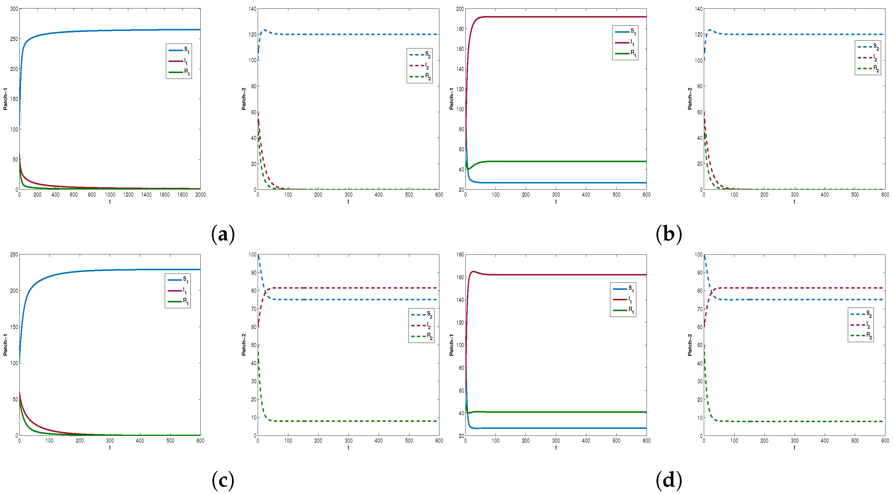
First, we discuss the situation when the population does not disperse between patches; Figure 2 depicts this scenario. Choosing ( β 1 , β 2 ) = ( 0.0003 , 0.00005 ) , it is observed that the system converges to an infection-free state for both the patches, we obtain a stable E 0 0 ( 166.67 , 0 , 0 , 240 , 0 , 0 ) , and the basic reproduction number ( R 0 ) becomes 0.62 (see Figure 2a). Now, if β 1 starts to increase, then E 0 0 becomes a saddle point and we can observe that the infection invades Patch-1. In Figure 2b, we obtain the basic reproduction number as R 0 = max { 6.25 , 0.2 } = 6.25 for β 1 = 0.003 and obtain a stable steady state containing an infection-free Patch-2 and infected Patch-1 E 1 0 ( 26.681 , 111.923 , 27.981 , 240 , 0 , 0 ) . On the other hand, if β 2 is increased instead of β 1 , then we can observe that the infection invades Patch-2. In Figure 2c, we obtain the basic reproduction number as R 0 = max { 0.625 , 1.999 } = 1.999 for β 2 = 0.0005 and obtain a stable steady state containing an infection-free Patch-1 and infected Patch-2 E 2 0 ( 166.67 , 0 , 0 , 120.084 , 108.931 , 10.893 ) . Now, if both β 1 and β 2 increase, then we have an infected system even if people do not disperse between the two patches. Figure 2d depicts the scenario at ( β 1 , β 2 ) = ( 0.003 , 0.0005 ) , where both Patch-1 and Patch-2 are infected with the disease and we obtain a stable E 0 ( 26.681 , 111.923 , 27.981 , 120.084 , 108.931 , 10.893 ) with R 0 = 6.25 ( > 1 ) .
Next, we discuss the case when the population from Patch-1 can disperse towards Patch-2 but cannot move back to Patch-1 again ( m 12 1 = m 12 2 = 0 ); Figure 3 depicts this scenario. Choosing ( β 1 , β 2 ) = ( 0.0003 , 0.00005 ) , it is observed that the system converges to an infection-free state for both patches, we obtain a stable E 0 m 21 ( 142.857 , 0 , 0 , 268.571 , 0 , 0 ) , and the basic reproduction number ( R 0 ) becomes 0.53 (see Figure 3a). From this situation, if β 1 starts to increase then E 0 m 21 becomes a saddle point and we can observe that the infection invades in Patch-1. In Figure 3b, we obtain the basic reproduction number as R 0 = max { 5.35 , 0.22 } = 6.25 for β 1 = 0.003 and obtain a stable steady state containing an infection-free Patch-2 and infected Patch-1 E 1 m 21 ( 26.681 , 107.574 , 23.905 , 247.727 , 0 , 2.391 ) . On the other hand, if β 2 is increased instead of β 1 , then we can observe that the infection invades in Patch-2, while Patch-1 remains infection-free. In Figure 3c, we obtain the basic reproduction number as R 0 = max { 0.54 , 2.24 } = 1.999 for β 2 = 0.0005 and obtain a stable steady state containing an infection-free Patch-1 and infected Patch-2 E 2 m 21 ( 142.857 , 0 , 0 , 120.084 , 134.885 , 13.488 ) . If both β 1 and β 2 increase, then we have an infected system even if people do not disperse between the two patches. Figure 3d depicts the scenario at ( β 1 , β 2 ) = ( 0.003 , 0.0005 ) , where both Patch-1 and Patch-2 are infected with the disease and we obtain a stable E m 21 ( 26.681 , 107.574 , 23.905 , 120.084 , 115.950 , 13.986 ) with R 0 = max { 5.35 , 2.24 } = 5.35 .
Next, we discuss the case when the population from Patch-2 can disperse towards Patch-1 but cannot move back to Patch-2 again ( m 21 1 = m 21 2 = 0 ); Figure 4 depicts this scenario. Choosing ( β 1 , β 2 ) = ( 0.0003 , 0.00005 ) , it is observed that the system converges to an infection-free state for both the patches, we obtain a stable E 0 m 12 ( 266.667 , 0 , 0 , 120 , 0 , 0 ) , and the basic reproduction number ( R 0 ) becomes 0.999 (see Figure 4a). Now, increasing the value of β 1 leads to instability as E 0 m 21 becomes saddle, and we can observe that the infection invades in Patch-1. In Figure 4b, we obtain the basic reproduction number as R 0 = max { 9.99 , 0.0999 } = 9.994 for β 1 = 0.003 and obtain a stable steady state containing an infection-free Patch-2 and infected Patch-1 E 1 m 12 ( 26.681 , 191.881 , 47.970 , 120 , 0 , 0 ) . On the other hand, if β 2 is increased instead of β 1 , then we can observe that the infection invades Patch-2 while Patch-1 remains infection-free. In Figure 4c, we obtain the basic reproduction number as R 0 = max { 0.999 , 1.599 } = 1.599 for β 2 = 0.0008 and obtain a stable steady state containing an infection-free Patch-1 and infected Patch-2 E 2 m 12 ( 229.293 , 0 , 0.248 , 75.053 , 81.479 , 7.949 ) . Now, if both β 1 and β 2 increase, then we have an infected system even if people do not disperse between the two patches. Figure 4d depicts the scenario at ( β 1 , β 2 ) = ( 0.003 , 0.0008 ) , where both Patch-1 and Patch-2 are infected with the disease and we obtain a stable E m 12 ( 26.681 , 161.999 , 40.748 , 75.053 , 81.479 , 7.949 ) with R 0 = max { 9.994 , 1.599 } = 9.994 .
Figure 5, shows the scenario when the population disperses between Patch-1 and Patch-2 ( m 0 ). Choosing ( β 1 , β 2 ) = ( 0.0003 , 0.00005 ) , it is observed that the system converges to an infection-free state for both patches, we obtain a stable E 0 m ( 246.154 , 0 , 0 , 144.615 , 0 , 0 ) , and the basic reproduction number ( R 0 ) becomes 0.923 (see Figure 5a). Now, this stable behavior of E 0 m switches with increasing value of β 1 as the equilibrium becomes saddle, and we obtain a scenario where the infection invades in Patch-1. In Figure 5b, we obtain the basic reproduction number as R 0 = max { 9.223 , 0.120 } = 9.994 for β 1 = 0.003 and obtain a stable steady state containing an infection-free Patch-2 and infected Patch-1 E 1 ( 26.681 , 190.103 , 42.360 , 124.734 , 0 , 4.133 ) . On the other hand, if β 2 is increased instead of β 1 , then we can observe that the infection invades Patch-2 while Patch-1 remains infection-free. In Figure 5c, we obtain the basic reproduction number as R 0 = max { 0.923 , 1.204 } = 1.204 for β 2 = 0.0005 and obtain a stable steady state containing an infection-free Patch-1 and infected Patch-2 E 2 m 12 ( 228.664 , 0 , 0.112 , 120.084 , 41.309 , 4.041 ) . Now, if both β 1 and β 2 increase, then we have an infected system even if people do not disperse between the two patches. Figure 5d depicts the scenario at ( β 1 , β 2 ) = ( 0.003 , 0.0005 ) , where both Patch-1 and Patch-2 are infected with the disease and we obtain a stable E m ( 26.681 , 187.033 , 41.699 , 120.084 , 8.371 , 4.885 ) with R 0 = max { 9.223 , 1.204 } = 9.223 . Moreover, from Figure 2d and Figure 5d it can be observed that although the infected population count has increased slightly in Patch-1 in the presence of population dispersal, it has significantly decreased in Patch-2. Moreover, the highest number of recovered individuals is obtained in Patch-1 ( R 1 ) when people can disperse between the patches.
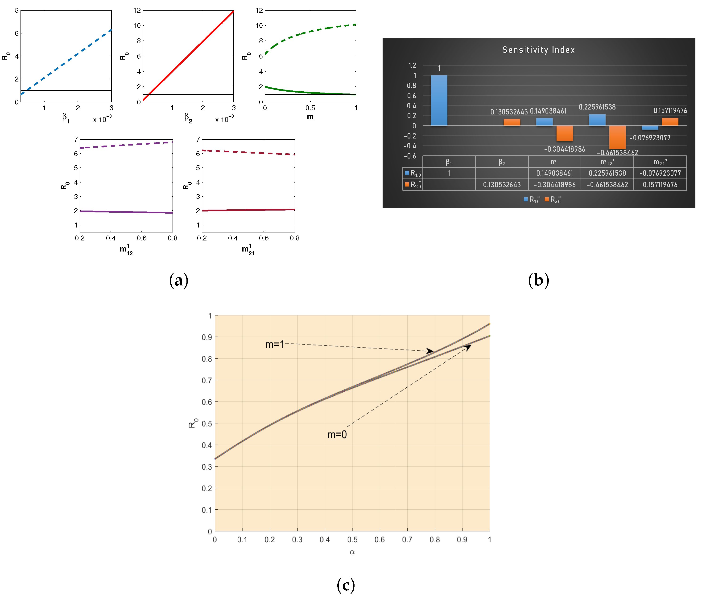
In Figure 6, we have analyzed the sensitivity of some of the system parameters in disease transmission, and have calculated corresponding sensitivity indices for the parametric values in Table 1 with m = 0.005 . The fact that the spread of the disease has a greater ascendancy for β 1 than β 2 can be observed in Figure 6a. Moreover, an increase in the disease transmission rates ( β 1 , β 2 ) actually proliferates the illness in a system, as the chances of spreading the infection become higher. On the other hand, for the chosen parametric values there is an inclination in the basic reproduction number for Patch-1 ( R 10 m ) and a declination for Patch-2 ( R 20 m ) with the increase in the population dispersal speed ( m ) . In addition, if more people move towards Patch-1 ( m 12 1 ) , then the prevalence of the illness in that patch is expanded, while in the other patch, the spread is somewhat more controlled. Furthermore, the inversely proportional relationship of m 21 1 with R 10 indicates that the epidemic situation in Patch-1 can be controlled by increasing people’s movement towards Patch-2. However, the infectivity in Patch-2 will increase in this case. Figure 6b contains the sensitivity indices for the parametric values in Table 1, which are calculated as follows: Γ β 1 = 1 , Γ β 2 = 0.130 , Γ m 1 = 0.149 , Γ m 2 = 0.304 , Γ m 12 1 1 = 0.226 , Γ m 12 1 2 = 0.462 , Γ m 21 1 1 = 0.077 and Γ m 21 1 2 = 0.157 , Γ α 1 = 0.3238 , Γ α 2 = 0.6290 . On the other hand, Figure 6c indicates that the spread of disease has an ascendency for increasing α .
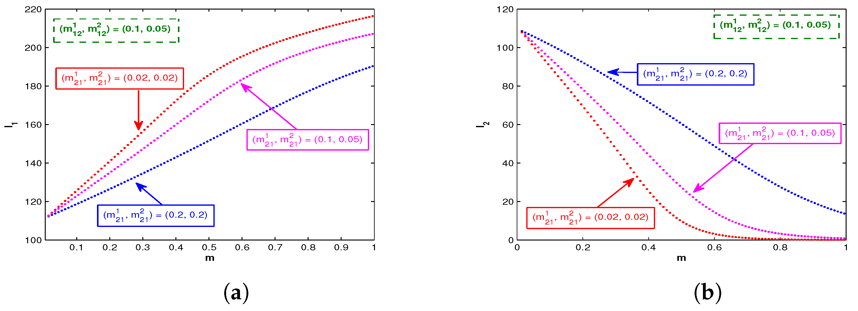
In Figure 7, we have plotted the count of infected people in Patch-1 ( I 1 ) and Patch-2 ( I 2 ) for different movement scenarios. We mainly considered three scenarios: (i) people move to Patch-2 in larger numbers ( m 12 1 < m 21 1 , m 12 2 < m 21 2 ) ; (ii) people move to Patch-1 with larger probabilities ( m 12 1 > m 21 1 , m 12 2 > m 21 2 ) ; and (iii) the probabilities are same for both patches ( m 12 1 = m 21 1 , m 12 2 = m 21 2 ) . Figure 7a shows that the count of infected people in Patch-1 is lowest when both susceptible and recovered people move to Patch-2, and that this situation leads to an inclination in the infectivity there (see Figure 7b). In fact, higher population dispersal probabilities (either of susceptible, recovered, or both) towards Patch-1 suppress the infection level in Patch-2 even for smaller dispersal speeds.

8. Numerical Simulation of System (2) without Implementation of Control Strategy

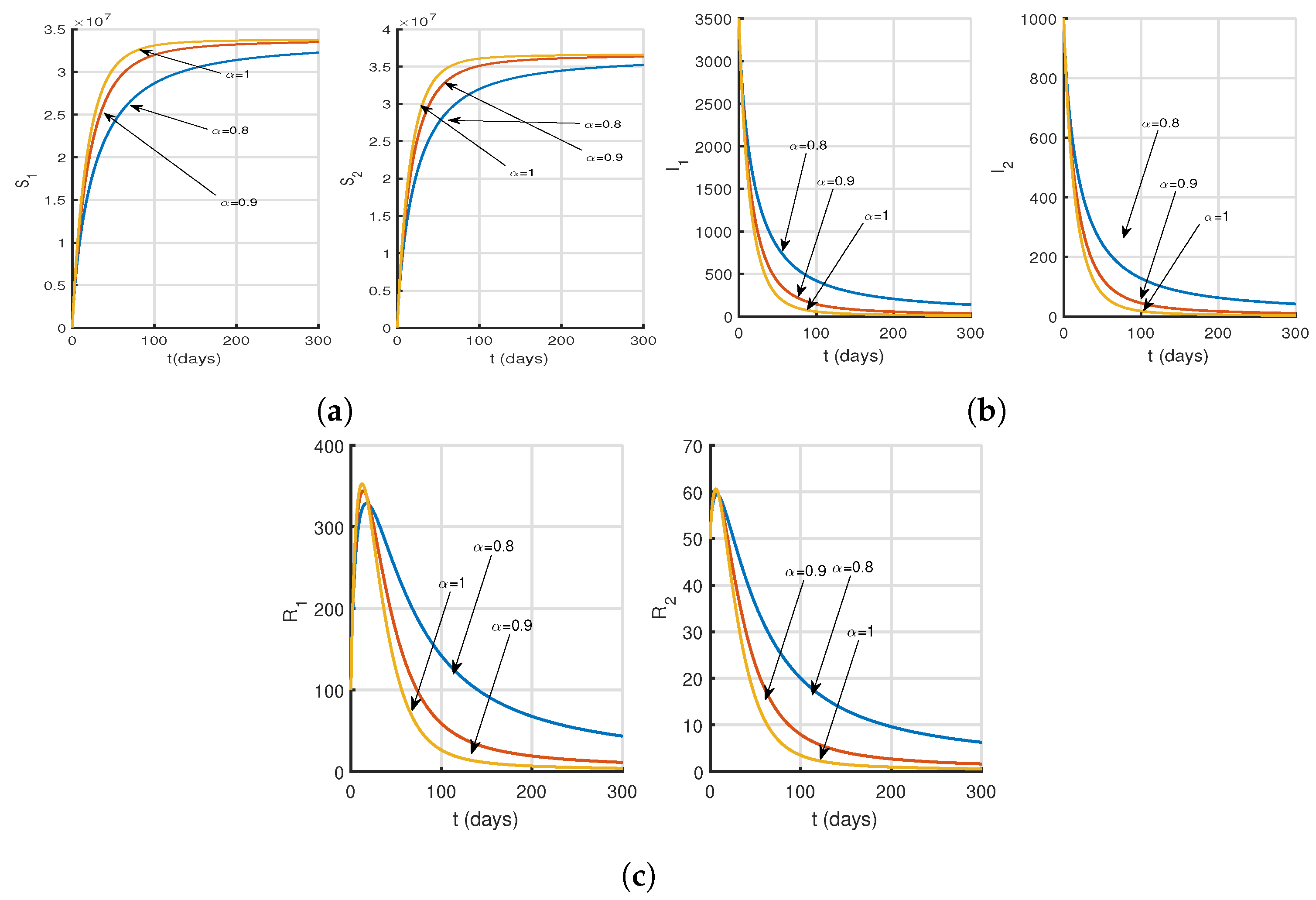
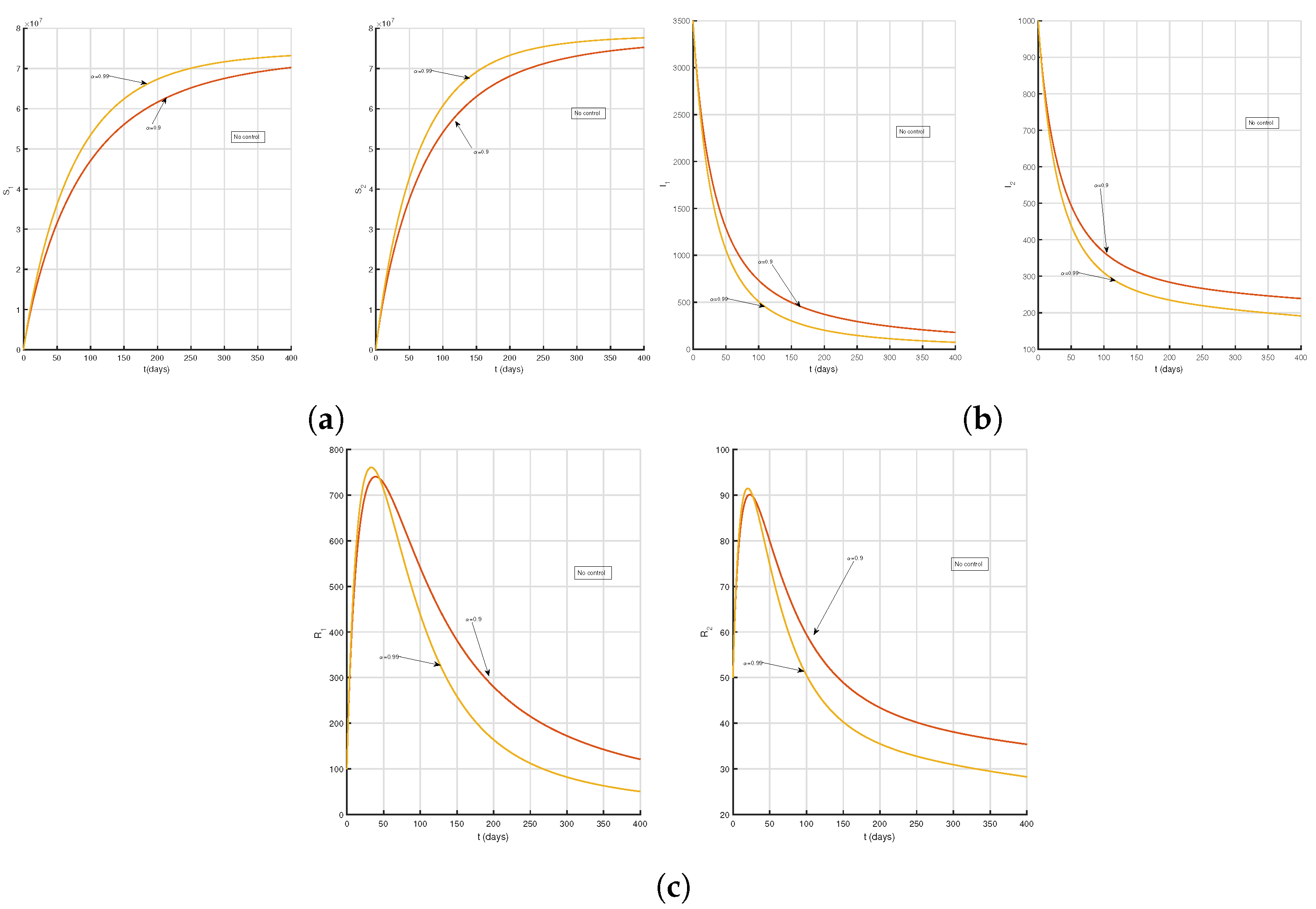
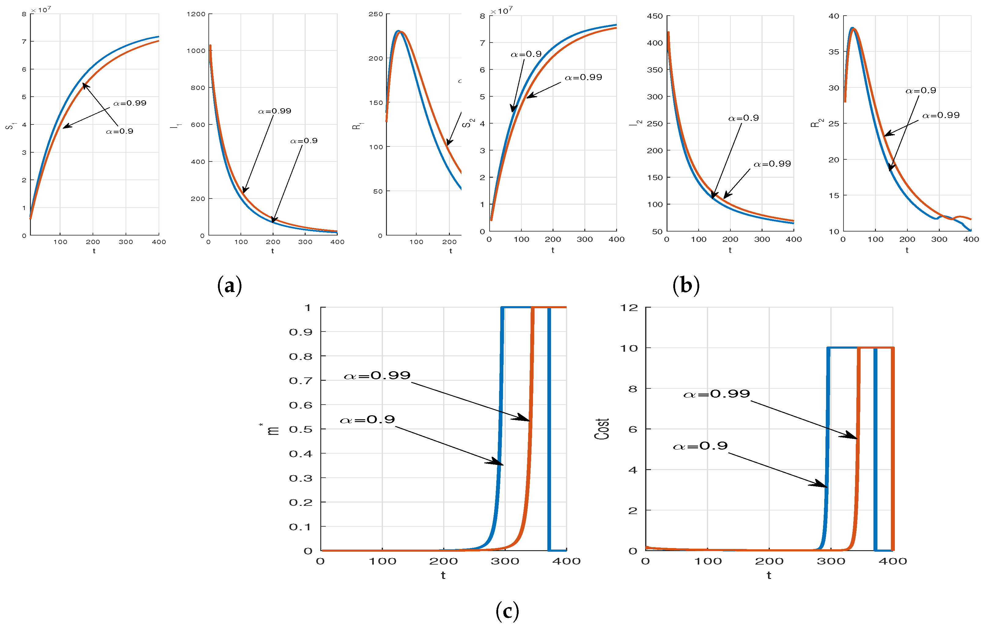
The numerical simulation of the system (2) is described in this section. We have used the FDE12 MatLab function, which is based on the Adams–Bashforth–Moulton algorithm introduced by Roberto Garrappa ([32]), and used a predictor-corrector method.
Case 1:
Consider the situation when there is no population dispersal between the patches (m = 0)
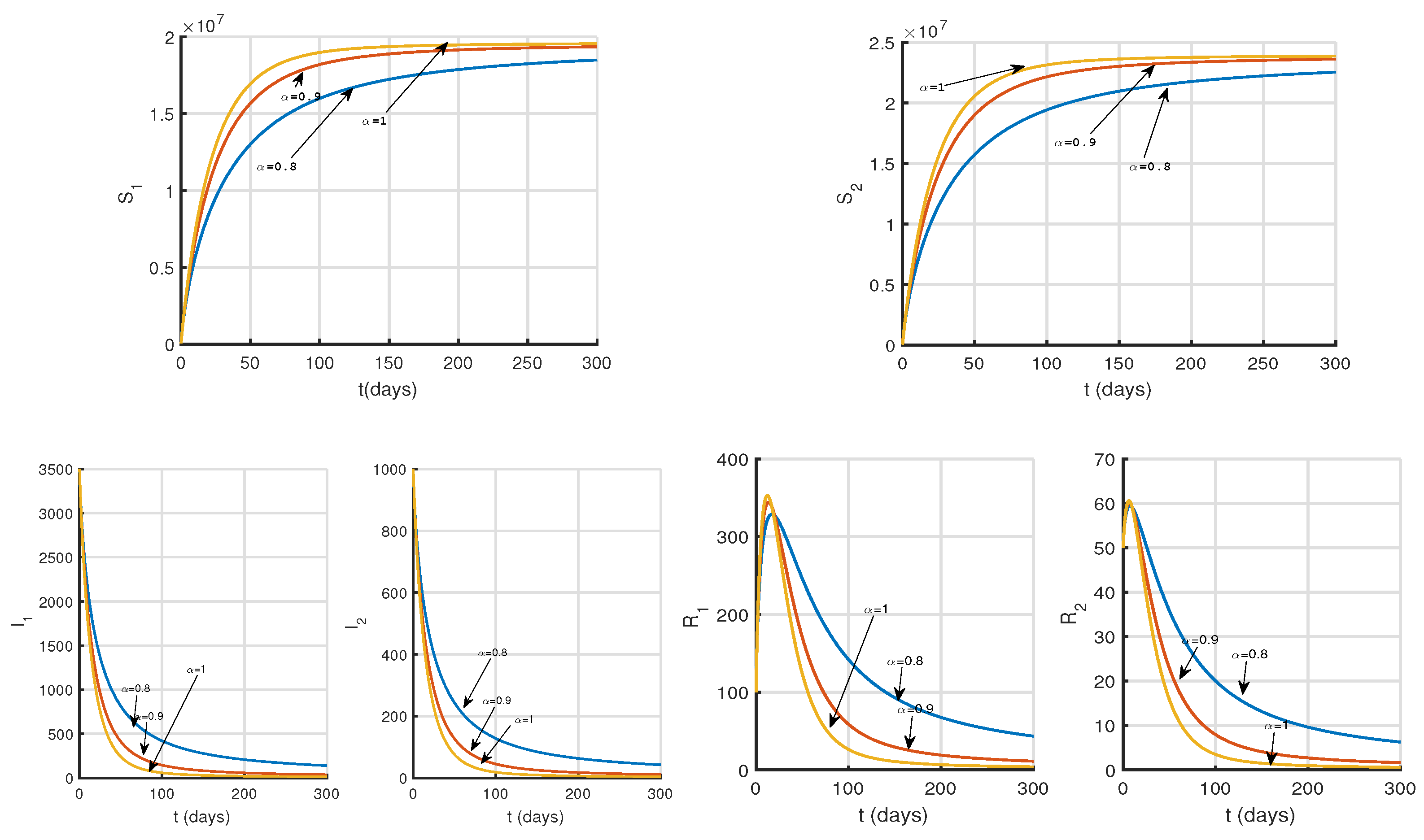
To analyze the dynamical behavior of all people, the values of the parameters in Table 1 are employed. The initial populations of both patches are taken in the following manner: S 1 = 50000 , I 1 = 2500 , R 1 = 50 , S 2 = 50000 , I 2 = 10000 , R 2 = 100 . Here, we are more concerned about the disease-free equilibrium. The population of the two patches has been considered as 100,000 people per patch, and we have taken t = 1 day as the time unit and T f = 300 . At first, we have considered μ 1 = 0.06 , μ 2 = 0.05 . From the direct calculation, we have R 0 = 0.1398 < 1 ; therefore, the disease-free equilibrium is stable (see Figure 8).
Case 2:
Consider the situation when there is population dispersal between the patches ( m 0 )
In this case, we fix m = 0.6 and consider Λ = 20 , Λ 2 = 25 , μ 1 = 0.19 , μ 2 = 0.15 ; then, we have R 0 = 0.1037 < 1 . The time series in Figure 9 shows the stability of the disease-free equilibrium.

9. Optimal Control Problem

The deterministic system (1) is further proposed with an effective control strategy to reduce the infection load. People’s movement between the two patches plays an important role in disease transmission. During an outbreak, people try to move back to their homes as soon as possible, and this behavior induces the transmission rate only. Furthermore, if people travel from a disease-prone area, it increases the chance of spreading the virus only. Imposing strict restrictions sometimes becomes necessary to control the continuous upsurge in transmission; thus, the dispersal speed of the population is considered as the control policy in this work, as it depends on the eruption of the infection and changes with time. Here, we study the characteristics of the applied time-dependent control policy mathematically. As the public authorities usually take immediate actions and impose strict restrictions only when the numbers of reported cases start to exceed the safe limit, instead of constant values, time-dependent dispersal rate function m ( t ) is considered here with 0 m ( t ) 1 . By implementing this control policy, the overall chances of becoming infected with the virus strain are lessened. Here, 1 indicates that people’s dispersal works with its fullest intensity, while 0 denotes full disconnection between the patches.
Our main focus is to determine the optimal control intervention with minimum implemented cost; hence, the region for the control intervention m ( t ) is provided as
Ψ = m ( t ) : m ( t ) [ 0 , 1 ] , t [ 0 , T f ] ,
where T f is the final time up to which the control policies are executed and m ( t ) is a measurable and bounded function.

Deduction of Total Cost Which Needs to Be Minimized Due to Dispersal

The total cost incurred to manage people’s emigration (or immigration) from (or to) the patches is provided by 0 T f [ w 1 I 1 ( t ) + w 2 I 2 ( t ) + w 3 m 2 ( t ) ] d t . The term ( w 1 I 1 ( t ) + w 2 I 2 ( t ) ) denotes the cost incurred in lost manpower because of the infected population in the patches. This is known as the opportunity loss, which includes productivity loss due to the infection. The term w 3 m 2 ( t ) represents the cost associated with managing the dispersal of population among the patches, which includes spreading information about the disease via different programs, informing the population about the importance of maintaining the proposed rules and regulations, etc. As this includes the cost of associated efforts towards convincing people, it is relatively higher. In this work, the nonlinearity term for the mitigation strategy is chosen up to the second order [33]. This work analyzes how the optimal control strategy representing people’s movement reduces the overall count of infected people in the system.
The following control problem is considered based on previous discussions, along with the cost functional J to be minimized [34]:
J [ m ( t ) ] = 0 T f w 1 I 1 ( t ) + w 2 I 2 ( t ) + w 3 m 2 ( t ) d t
subject to the model system
d S 1 d t = Λ 1 β 1 S 1 I 1 μ 1 S 1 + η 1 R 1 + m ( t ) ( m 12 1 S 2 m 21 1 S 1 ) , d I 1 d t = β 1 S 1 I 1 ( μ 1 + δ 1 ) I 1 γ 1 I 1 , d R 1 d t = γ 1 I 1 μ 1 R 1 η 1 R 1 + m ( t ) ( m 12 2 R 2 m 21 2 R 1 ) , d S 2 d t = Λ 2 β 2 S 2 I 2 μ 2 S 2 + η 2 R 2 + m ( t ) ( m 21 1 S 1 m 12 1 S 2 ) , d I 2 d t = β 2 S 2 I 2 ( μ 2 + δ 2 ) I 2 γ 2 I 2 , d R 2 d t = γ 2 I 2 μ 2 R 2 η 2 R 2 + m ( t ) ( m 21 2 R 1 m 12 2 R 2 )
with initial conditions S 1 ( 0 ) > 0 , I 1 ( 0 ) > 0 , R 1 ( 0 ) > 0 , S 2 ( 0 ) > 0 , I 2 ( 0 ) > 0 and R 2 ( 0 ) > 0 . We have already considered p i = ( μ i + δ i + γ i ) for i = 1 , 2 and p j = ( μ j 2 + η j 2 ) for j = 3 , 4 . The functional J denotes the total incurred cost as stated, and the integrand
L ( S 1 , I 1 , R 1 , S 2 , I 2 , R 2 , m ( t ) ) = w 1 I 1 ( t ) + w 2 I 2 ( t ) + w 3 m 2 ( t )
denotes the cost at time t. The positive parameters w 1 , w 2 , a n d w 3 are weight constants balancing the units of the integrand [33,35]. The optimal control interventions m exist in Ψ , and mainly minimize the cost functional J.
Theorem 13.
The optimal control intervention m in Ψ of the control systems (5) and (6) exists such that J ( m ) = min [ J ( m ) ] .
Proof. 
The proof is presented in Appendix A. □
Theorem 14.
For the optimal control m and corresponding optimal states ( S 1 m , I 1 m , R 1 m , S 2 m , I 2 m , R 2 m ) of system (6), there exist adjoint variables λ = λ 1 , λ 2 , λ 3 , λ 4 , λ 5 , λ 6 R 6 satisfying the canonical equations:
d λ 1 d t = λ 1 [ β 1 I 1 + μ 1 + m m 21 1 ] λ 2 [ β 1 I 1 ] λ 4 [ m m 21 1 ] , d λ 2 d t = w 1 + λ 1 [ β 1 S 1 ] λ 2 [ β 1 S 1 p 1 ] λ 3 [ γ 1 ] , d λ 3 d t = λ 1 [ η 1 ] + λ 3 [ p 3 + m m 21 2 ] λ 6 [ m m 21 2 ] , d λ 4 d t = λ 1 [ m m 12 1 ] + λ 4 [ β 2 I 2 + μ 2 + m m 12 1 ] λ 5 [ β 2 I 2 ] , d λ 5 d t = w 2 + λ 4 [ β 2 S 2 ] λ 5 [ β 2 S 2 p 2 ] λ 6 [ γ 2 ] , d λ 6 d t = λ 3 [ m m 12 2 ] λ 4 [ η 2 ] + λ 6 [ p 4 + m m 12 2 ] ,
with transversality conditions λ i ( T f ) = 0 for i = 1 , 2 , , 6 . The corresponding optimal control m which minimizes J ( m ) in Ψ is provided as follows:
m = min max 0 , ( λ 4 λ 1 ) ( m 12 1 S 2 m m 21 1 S 1 m ) + ( λ 6 λ 3 ) ( m 12 2 R 2 m m 21 2 R 1 m ) 2 w 3 , 1 .
Proof. 
The proof is presented in Appendix A. □
Now, the model system in the Caputo fractional system with the implemented control intervention is as follows:
D α 0 C S 1 = Λ 1 β 1 S 1 I 1 μ 1 S 1 + η 1 R 1 + m ( t ) ( m 12 1 S 2 m 21 1 S 1 ) , D α 0 C I 1 = β 1 S 1 I 1 ( μ 1 + δ 1 ) I 1 γ 1 I 1 , D α 0 C R 1 = γ 1 I 1 μ 1 R 1 η 1 R 1 + m ( t ) ( m 12 2 R 2 m 21 2 R 1 ) , D α 0 C S 2 = Λ 2 β 2 S 2 I 2 μ 2 S 2 + η 2 R 2 + m ( t ) ( m 21 1 S 1 m 12 1 S 2 ) , D α 0 C I 2 = β 2 S 2 I 2 ( μ 2 + δ 2 ) I 2 γ 2 I 2 , D α 0 C R 2 = γ 2 I 2 μ 2 R 2 η 2 R 2 + m ( t ) ( m 21 2 R 1 m 12 2 R 2 )
with initial conditions S 1 ( 0 ) > 0 , I 1 ( 0 ) > 0 , R 1 ( 0 ) > 0 , S 2 ( 0 ) > 0 , I 2 ( 0 ) > 0 , and R 2 ( 0 ) > 0 .
Theorem 15.
For the optimal control m and corresponding optimal states ( S 1 m , I 1 m , R 1 m , S 2 m , I 2 m , R 2 m ) of system (9), there exist adjoint variables λ = λ 1 , λ 2 , λ 3 , λ 4 , λ 5 , λ 6 R 6 satisfying the canonical equations:
D α 0 R L λ 1 = λ 1 [ β 1 I 1 + μ 1 + m m 21 1 ] λ 2 [ β 1 I 1 ] λ 4 [ m m 21 1 ] , D α 0 R L λ 2 = w 1 + λ 1 [ β 1 S 1 ] λ 2 [ β 1 S 1 p 1 ] λ 3 [ γ 1 ] , D α 0 R L λ 3 = λ 1 [ η 1 ] + λ 3 [ p 3 + m m 21 2 ] λ 6 [ m m 21 2 ] , D α 0 R L λ 4 = λ 1 [ m m 12 1 ] + λ 4 [ β 2 I 2 + μ 2 + m m 12 1 ] λ 5 [ β 2 I 2 ] , D α 0 R L λ 5 = w 2 + λ 4 [ β 2 S 2 ] λ 5 [ β 2 S 2 p 2 ] λ 6 [ γ 2 ] , D α 0 R L λ 6 = λ 3 [ m m 12 2 ] λ 4 [ η 2 ] + λ 6 [ p 4 + m m 12 2 ] ,
where D α 0 R L is the α-ordered Riemann–Liouville derivative with initial point 0 and transversality conditions λ i ( T f ) = 0 for i = 1 , 2 , , 6 . The corresponding optimal control m which minimizes J ( m ) in Ψ is provided as follows:
m = min max 0 , ( λ 4 λ 1 ) ( m 12 1 S 2 m m 21 1 S 1 m ) + ( λ 6 λ 3 ) ( m 12 2 R 2 m m 21 2 R 1 m ) 2 w 3 , 1 .
Proof. 
The proof is similar to the proof of Theorem 14 mentioned in the Appendix A.2 of Appendix A. □

10. Numerical Simulation of the Optimal Control Problem (6)

In the proposed system (6), we have considered the population dispersal speed ( m ) as the control intervention in order to analyze its impact on reducing the infection level. The control intervention is assumed to be time-independent, as it changes according to the disease prevalence, fatality, and governmental rules and restrictions. Through employing a forward–backward sweep approach, numerical simulations have been carried out to demonstrate the effects of different control strategies on the behavior of the system [36,37]. The parametric values are chosen from Table 1 along with β 1 = 0.003 , β 2 = 0.005 , m = 0.005 , and the positive weight constants are taken as w 1 = 1 , w 2 = 25 , and w 3 = 100 . Additionally, it is presumed that the control techniques will be used consistently for two months, or T f = 21 days. The initial population size is chosen as follows: S 1 ( 0 ) = 300 , I 1 ( 0 ) = 175 , R 1 ( 0 ) = 100 , S 2 ( 0 ) = 100 , I 2 ( 0 ) = 75 , R 2 ( 0 ) = 75 .
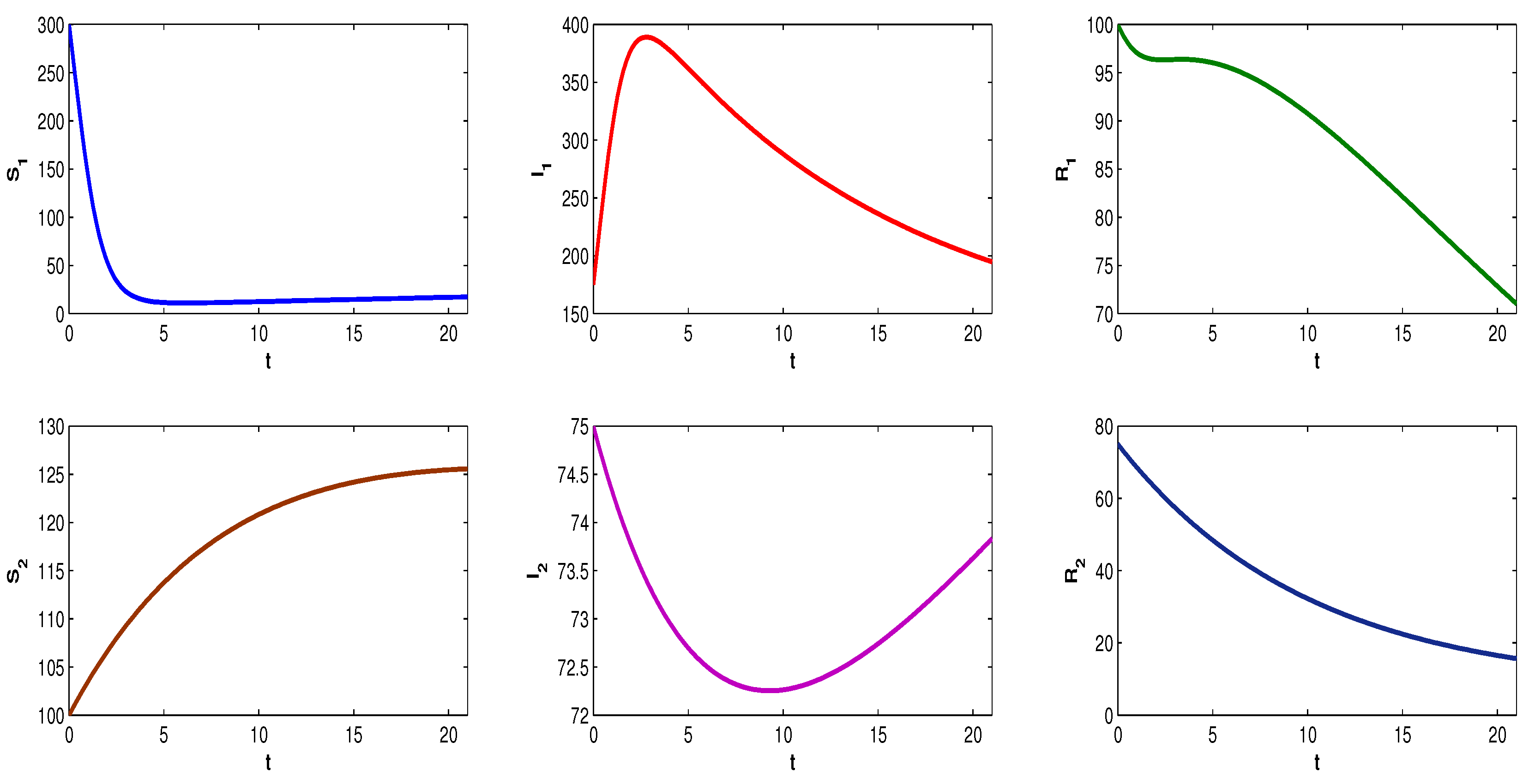
The dynamics of model (6) when the dispersal speed is chosen as a constant value instead of a time-dependent control measure are shown in Figure 10. In this scenario, the population size is ( 17.20 , 194.74 , 71.02 , 125.56 , 73.83 , 15.66 ) at T f = 21 .
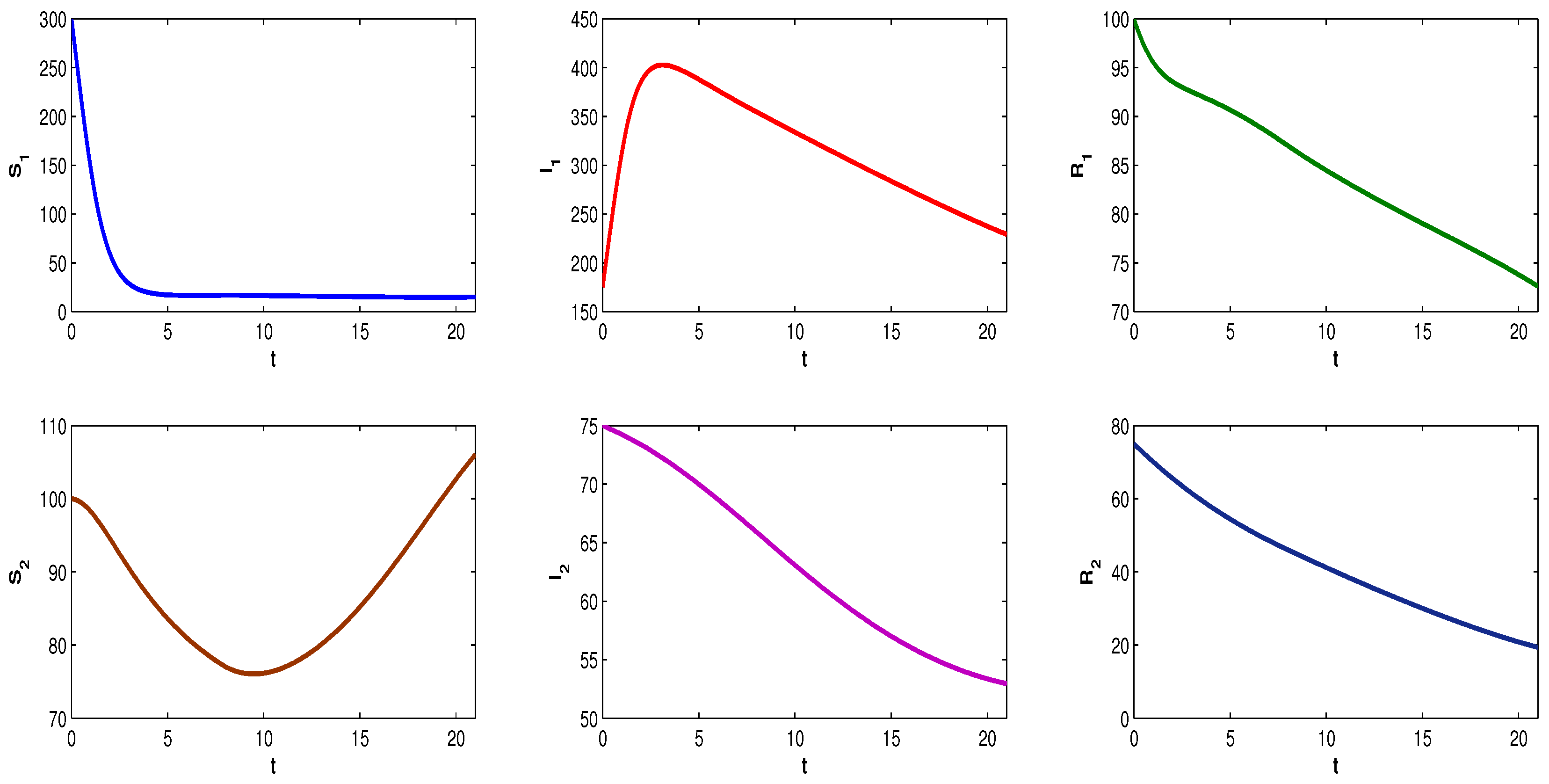
If the control strategy is properly implemented through people’s dispersal (or migration) strategy, the burden of the infection may be managed more effectively. Hence, we have emphasized the fact that susceptible and recovered people move or disperse between Patch-1 and Patch-2 according to disease severity, allowing the increased disease transmission to be curbed. The population trajectories in the presence of the control strategy are shown in Figure 11, and at T f = 21 , the population is represented as ( 14.92 , 229.11 , 72.59 , 106.01 , 52.95 , 19.34 ) . In this situation, the count of the infected population increases in Patch-1 and declines in Patch-2. Surprisingly, we find the highest number of recovery cases in both patches. Higher recovery results in a slightly lower susceptible population count in the patches than in the scenario where dispersal speed is not used as a control approach. Figure 12b reveals the optimal graphs of the control intervention, where can be seen that its intensity remains at the highest level for almost 10 days, then starts to diminish in the last few days.
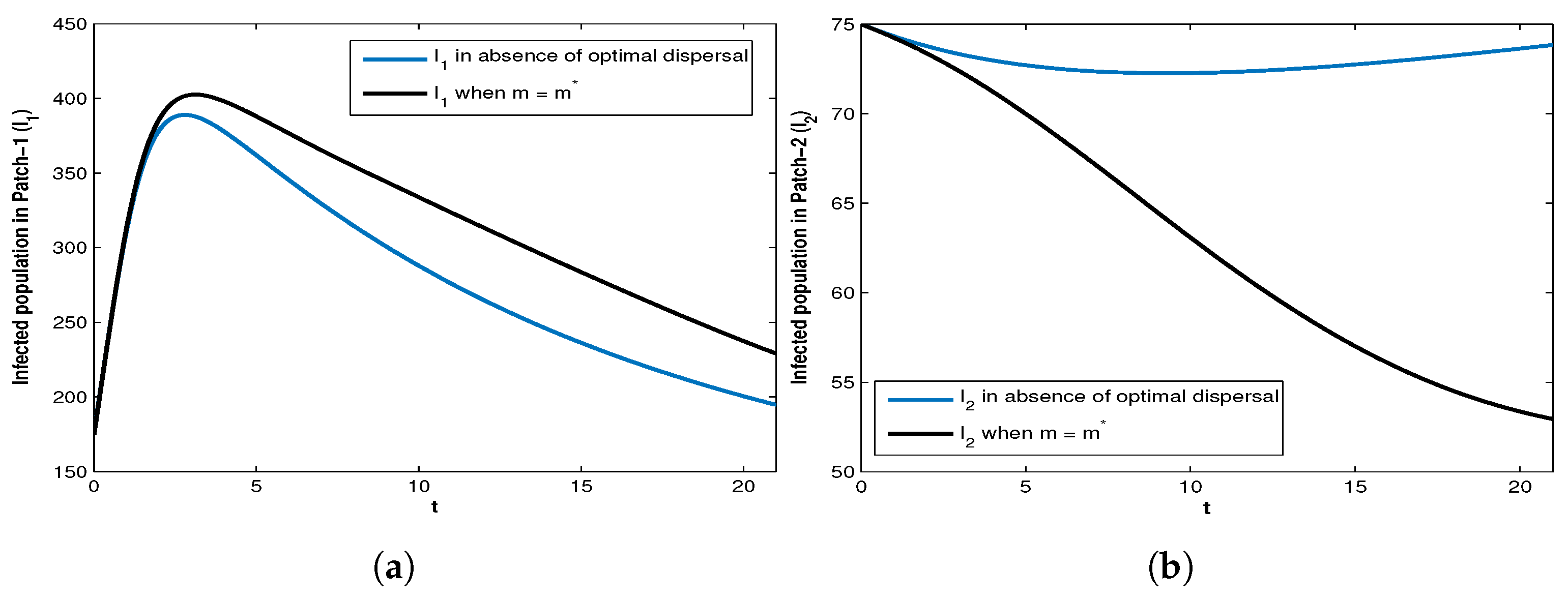
The significance of an implemented control measure is determined by how cost-effective it is. Figure 12 and Figure 13 illustrate the impact of the time-dependent control measure ( m ( t ) ) on the cost design analysis ( J ) (Figure 12a) and the infected population count of both patches ( I 1 , I 2 ) (Figure 13). Without the control measure, the cost is due to the impact of the disease load on the production loss. When the control measure is not implemented, the infected population in Patch-1 is high enough, as is that in Patch-2; in fact, it is at its maximum count, which results in higher opportunity loss and leads to a rise in the economic burden. It is shown in Figure 13a that although there is a small inclination in I 1 in the presence of optimal dispersal, we have the fewest number of infected people in Patch-2 in the presence of this control policy, and this situation makes the optimal cost much lower. This finding indicates that implementing the control strategy results in a lower cost profile than not implementing the intervention. Thus, it may be said that the control policy is financially viable.

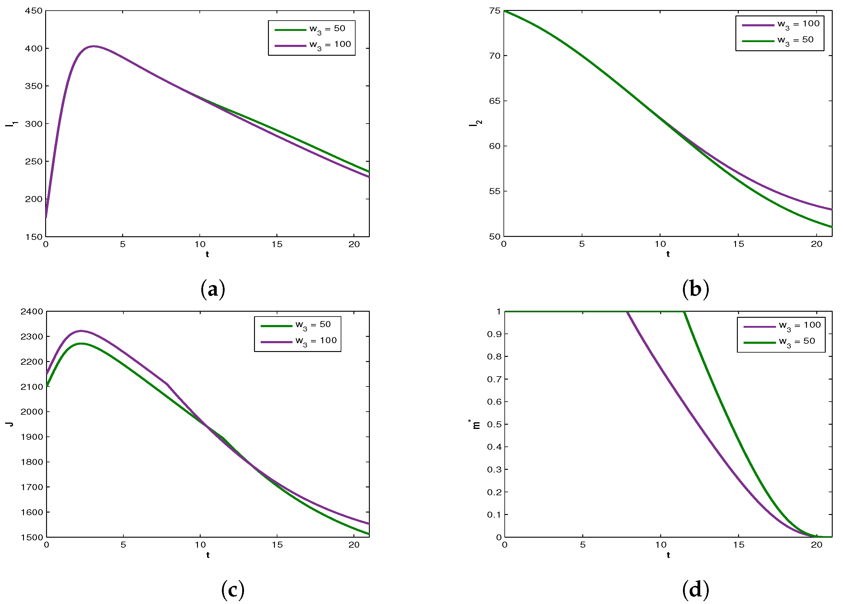
10.1. Effect of the Weight Constant w 3 on the Optimal Control Policy

When determining the weight that needs to be applied to a particular control, weight constants are essential. Here, we vary the weight constant w 3 in order to identify its effectiveness. Figure 14c illustrates that placing higher weight on migration results in an upsurge in overall cost. Moreover, increasing w 3 decreases the infection level in Patch-1 but spreads the infectivity in Patch-2 (see Figure 14a,b). It can be seen in Figure 14d that if the related weight ( w 3 ) is larger, then more effort on the part of the control is needed to lower the cost and total number of infected people.

10.2. Effect of Behavioral Changes and People’s Awareness on Disease Transmission When m 0

In this work, we have mainly focused on the dynamical behavior of an SIRS model in which the population disperses between two patches. In Figure 15, we have tried to show how the infection level is affected when people’s behavioral changes, mainly the population’s awareness towards preventive measures or precautionary measures, are taken into consideration in the presence of optimal dispersal. It can be observed that the count of the infected population in both patches ( I 1 , I 2 ) is reduced when people start to pay attention to restrictions and precautions. Figure 15c shows that if people adopt proper behavioral changes, then a comparatively lower effort in terms of the control policy is required to reduce the count of infected individuals in the system.

11. Numerical Simulation of the Optimal Control Problem (9)

In this section, we discuss the effect of optimal control on the disease transmission dynamics. We can set the dispersal rate (m) under the control such that the cost function is minimized. Here, we have assumed that w 1 = 10 , w 2 = 10 , w 3 = 100 , and Λ 1 = 12 , Λ 2 = 15 . All other parametric values are taken from Table 1. We performed the simulation for α = 0.9 , α = 0.99 . We have assumed t = 1 day as a time unit and T f = 400 .
We have developed a fractional order optimal control problem using an iterative approach (Euler’s forward and backward) in the MatLab interface [32,38]. The procedure is summarized below. A two-point boundary value problem with a set of fractional-order differential equations defines the optimality of the system (9). The initial value system (9) is an initial value problem and the adjoint system is a boundary value problem. The state system is solved using the forward iteration approach, while the co-state system is solved using the backward iteration method using the Matlab code presented below.
The state system (9) is solved using the following iterative scheme:
S 1 ( i ) = [ Λ β S 1 ( i 1 ) I 1 ( i 1 ) μ 1 S 1 ( i 1 ) + η 1 R 1 ( i 1 ) + m ( i 1 ) ( m 12 1 S 2 ( i 1 ) m 21 1 S 1 ( i 1 ) ) ] h α j = 1 i c ( j ) S ( i j ) I 1 ( i ) = [ β 1 S 1 ( i 1 ) I 1 ( i 1 ) ( μ 1 + δ 1 + γ 1 ) I 1 ( i 1 ) ] h α j = 1 i c ( j ) I 1 ( i j ) R 1 ( i ) = [ γ 1 I 1 ( i 1 ) μ 1 R 1 ( i 1 ) η 1 R 1 ( i 1 ) + m ( i 1 ) ( m 12 2 R 2 ( i 1 ) m 21 2 R 1 ( i 1 ) ) ] h α j = 1 i c ( j ) R 1 ( i j ) S 2 ( i ) = [ Λ 2 β 2 S 2 ( i 1 ) I 2 ( i 1 ) μ 2 S 2 ( i 1 ) + η 2 R 2 ( i 1 ) + m ( i 1 ) ( m 21 1 S 1 ( i 1 ) m 12 1 S 2 ( i 1 ) ) ] h ε j = 1 i c ( j ) S 2 ( i j ) I 2 ( i 1 ) = [ β 2 S 2 ( i 1 ) I 2 ( i 1 ) ( μ 2 + δ 2 ) I 2 ( i 1 ) γ 2 I 2 ( i 1 ) ] h α j = 1 i c ( j ) I 2 ( i j ) R 2 = [ γ 2 I 2 μ 2 R 2 η 2 R 2 + m ( t ) ( m 21 2 R 1 m 12 2 R 2 ) ] h α j = 1 i c ( j ) R 2 ( i j )
where c ( 0 ) = 1 , c ( j ) = ( 1 1 + α j ) c ( j 1 ) , j 1 , and h α is the length of the time step; moreover, S 1 ( i ) is the value of S 1 ( t ) at i t h iteration. The last term of each of the above system of equations stands for memory. The adjoint system (10) is solved using the backward iteration method with terminal conditions λ i ( T f ) = 0 , i = 1 , 2 , 3 , 4 with the following iterative scheme:
λ 1 ( i ) = [ λ 1 ( i 1 ) [ β 1 I 1 ( i 1 ) + μ 1 + m ( i 1 ) m 21 1 ] λ 2 ( i 1 ) [ β 1 I 1 ( i 1 ) ] λ 4 ( i 1 ) [ m m 21 1 ] ] h α j = 1 i c ( j ) λ 1 ( i j ) λ 2 ( i ) = [ w 1 + λ 1 ( i 1 ) [ β 1 S 1 ( i 1 ) ] λ 2 [ β 1 S 1 ( i 1 ) p 1 ] λ 3 ( i 1 ) γ 1 ] h α j = 1 i c ( j ) λ 2 ( i j ) λ 3 ( i ) = [ λ 1 ( i 1 ) [ η 1 ] + λ 3 ( i 1 ) [ p 3 + m ( i 1 ) m 21 2 ] λ 6 ( i 1 ) [ m m 21 2 ] ] h α j = 1 i c ( j ) λ 3 ( i j ) λ 4 ( i ) = [ λ 1 ( i 1 ) [ m ( i 1 ) m 12 1 ] + λ 4 [ β 2 I 2 + μ 2 + m ( i 1 ) m 12 1 ] λ 5 ( i 1 ) [ β 2 I 2 ( i 1 ) ] ] h α j = 1 i c ( j ) λ 4 ( i j ) λ 5 ( i ) = [ w 2 + λ 4 ( i 1 ) [ β 2 S 2 ( i 1 ) ] λ 5 ( i 1 ) [ β 2 S 2 ( i 1 ) p 2 ] λ 6 ( i 1 ) [ γ 2 ] ] h α j = 1 i c ( j ) λ 5 ( i j ) λ 6 ( i ) = [ λ 3 ( i 1 ) [ m ( i 1 ) m 12 2 ] λ 4 ( i 1 ) [ η 2 ] + λ 6 ( i 1 ) [ p 4 + m ( i 1 ) m 12 2 ] ] h α j = 1 i c ( j ) λ 6 ( i j )
where p j = ( μ j 2 + η j 2 ) for j = 3 , 4 . The system below updates the optimal control:
m ( i ) = min max 0 , ( λ 4 ( i 1 ) λ 1 ( i 1 ) ) ( m 12 1 S 2 ( i 1 ) m 21 1 S 1 ( i 1 ) ) + ( λ 6 ( i 1 ) λ 3 ( i 1 ) ) ( m 12 2 R 2 ( i 1 ) m 21 2 R 1 ( i 1 ) ) 2 w 3 , 1 .
We have developed MatLab code using the above algorithm and chose h = 0.02 throughout the numerical simulations. The number of infected people in both patches can be gradually reduced by controlling m . The optimal value of the migration rate quickly approaches 1 as the order of the derivative α increases. The effect of the other parameters has already been mentioned in Section 10. In this section, we have only observed the impact of the order of derivatives in the control system. Figure 16 depicts the time series of the S, I, and R variables for α = 0.9 , 0.99 . Figure 17 provides a comparison of the time series of the system variables along with the control variable and cost function. It is apparent that the optimal stage can be archived quickly for a lower value of α .

12. Conclusions

When it comes to population dispersal, infectious diseases tend to be a cause for concern. In densely populated areas, respiratory diseases such as flu or COVID-19 have a tendency to be highly infectious, as they can spread very quickly. There are several other aspects that causes high transmission. It includes mode of transmission, period of infectivity, efficacy of implemented preventative measures, etc., which can be taken into account. In order to control the spread of disease during population movement or traveling, public health is essential. The migration of people, which has increased with time and growing socioeconomic conditions, expanding tourism, etc., acts as a contributing factor. This movement alleviates the spread of an infectious disease; thus, analyzing an epidemic model in the presence of population dispersal is of utmost importance.
In this work, a compartmental SIRS model has been proposed in a two-patch environment, where it is assumed that only susceptible and recovered populations are allowed to disperse between the patches. A deterministic model and a fractional-order system are analyzed here in order to observe the detailed dynamical scenario. Four situations are taken into consideration while analyzing the equilibrium points of the system: (i) no dispersal between the patches; (ii) people can travel from Patch-1 to Patch-2 but cannot move back to Patch-1; (iii) people can travel from Patch-2 to Patch-1 but cannot move back to Patch-2; and (iv) people can freely disperse between the two patches. In these cases, we respectively reach a disease-free equilibrium state, an infection-free Patch-2 and infected Patch-1 state, an infection-free Patch-1 and infected Patch-2 state, and an infected state in which both patches are infected. The numerical scenario shows that the disease transmission rates in both patches play significant roles in the stability of the system, as adjusting these parameters decides whether the disease will invade the patch or not. It is notable that although the infected population count increases slightly in Patch-1 in the presence of population dispersal, it significantly decreases in Patch-2. For the chosen parametric values, the results depict that there is an inclination in the basic reproduction number for Patch-1 ( R 10 m ) and a declination for Patch-2 ( R 20 m ) with the increase in the population dispersal speed ( m ) . In the later part of the paper, a corresponding optimal control problem is formulated in which the dispersal speed of the population is considered to be time-dependent instead of a constant value. The numerical scenario reveals that the count of the infected population increases in Patch-1 and declines in Patch-2 in the presence of optimal dispersal, and that the highest number of recovery cases has been obtained in both patches.
In the model simulation, fractional order has a noticeable impact. It is noteworthy that when the derivative order decreases, the recovery rate increases. Both patches have a comparable rise in the infected population, although at a lower derivative rate. In the control situation, the order of derivatives is less, and the optimal state is reached faster. These effects can be quite useful when trying to fit actual data into real-life scenarios.
While the model proposed here has shown some interesting dynamical behavior, there are many remaining items that can be implemented later as an extension of this work. In this work, we have only dealt with the deterministic and fractional approaches; environmental stochasticity has not been incorporated here. It would be interesting to explore whether Gaussian noise plays a significant role in this dispersed epidemic model. Secondly, we have only considered scenarios in which susceptible and recovered people are allowed to move between two patches; any asymptomatic or pre-symptomatic stage has not been considered here. It is quite evident that people belonging to these stages shall also move between the patches, and so the future researchers can possibly observe the impact of this movement on the dynamics of the system. Moreover, a certain amount of time is required for a person to be infected with a certain type of virus. As it is not an instantaneous process, consideration of a delay parameter can make the model more realistic. The present work can be studied further by incorporating the facts mentioned above in order to observe various realistic dynamical behaviors.
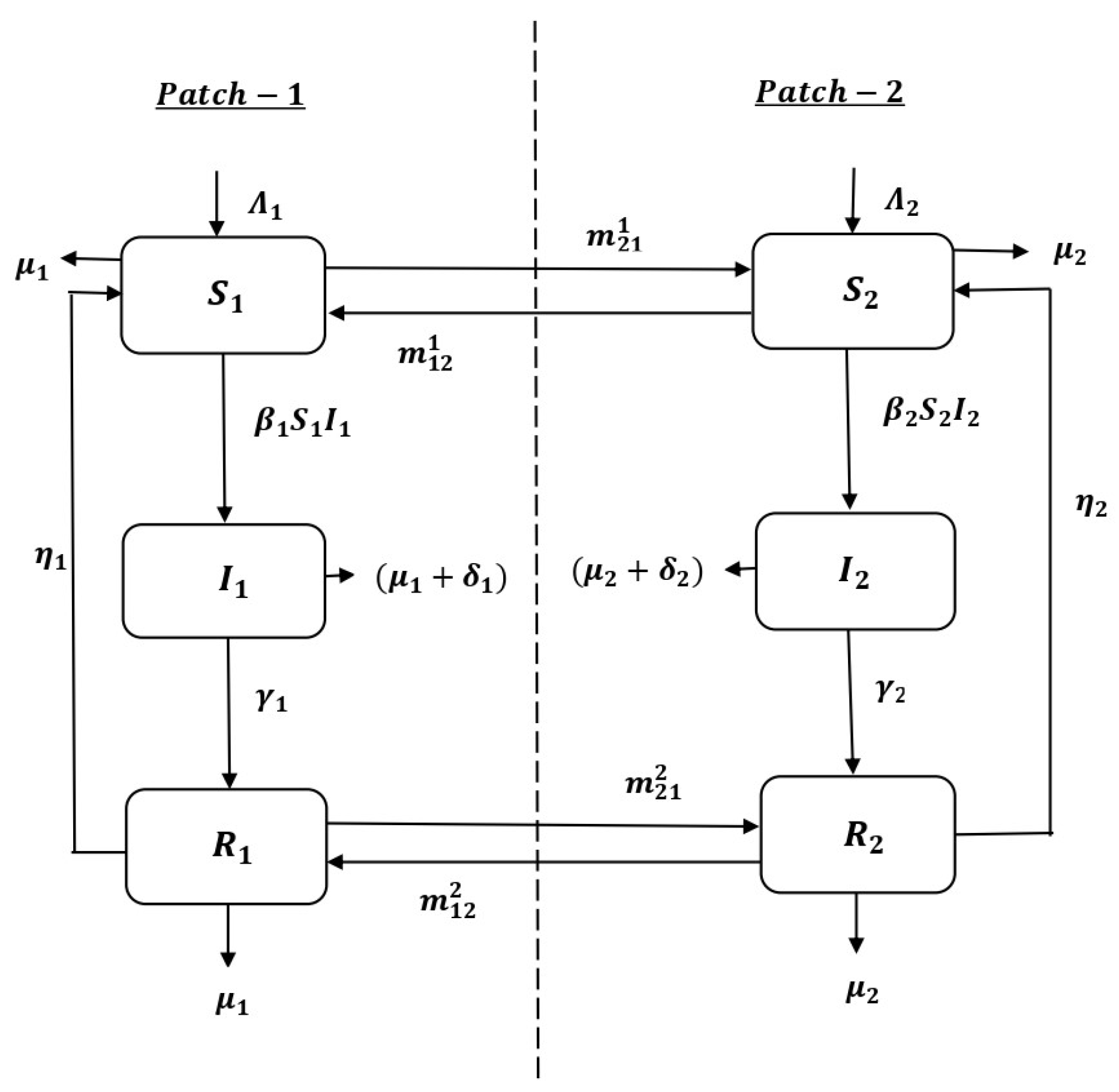
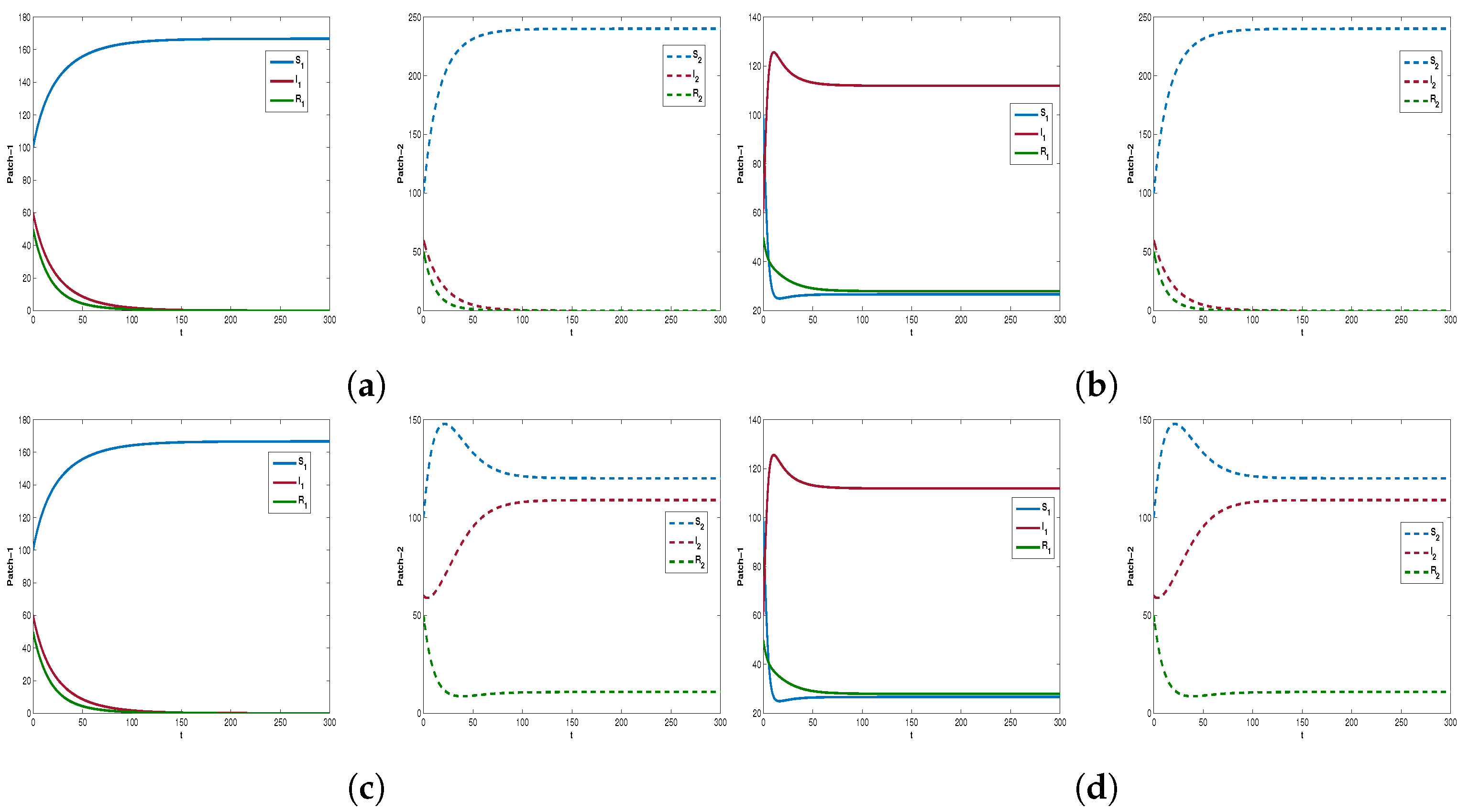
Author Contributions

All the authors have participate equally in all the aspects of this paper: conceptualization, methodology, investigation, formal analysis, writing—original draft preparation, writing—review and editing. All authors have read and agreed to the published version of the manuscript.

Funding

This research received no external funding.

Data Availability Statement

The data used to support the findings of the study are available within the article.

Acknowledgments

The authors are grateful to the anonymous referees, for their careful reading, valuable comments, and helpful suggestions, which have helped to significantly improve the presentation of this work.

Conflicts of Interest

The authors state that they do not have any conflicts of interest in respect of this study.

Appendix A

Appendix A.1. Existence of Optimal Control Functions

Here, the existence of optimal control interventions which minimize the cost functional within a finite time interval are provided.
Proof of Theorem 13.
In model (6), the overall population N = N 1 ( t ) + N 2 ( t ) is assumed to be N = S 1 + I 1 + R 1 + S 2 + I 2 + R 2 .
Thus , we have d N d t ( Λ 1 + Λ 2 ) μ 1 N 1 μ 2 N 2 Λ μ N 0 < N ( t ) Λ μ + N ( 0 ) Λ μ e μ t
where Λ = Λ 1 + Λ 2 , μ = min { μ 1 , μ 2 } and N ( 0 ) = S 1 ( 0 ) + I 1 ( 0 ) + R 1 ( 0 ) + S 2 ( 0 ) + I 2 ( 0 ) + R 2 ( 0 ) . Because t , 0 < N ( t ) Λ μ + ϵ , for any ϵ > 0 .
Here, system (6) has a bounded solution when control interventions are present in the system and the right side functions of the system are Lipschitzian in Ψ . Thus, control system (6) has a non-trivial solution in Ψ per the P i c a r d - L i n d e l o ¨ f theorem [39].
Here, Ψ is a closed convex set within which the control variables lie, and system (6) can be written as linear in control variable m with coefficients depending on the state variables. Moreover, the integrand L ( S 1 , I 1 , R 1 , S 2 , I 2 , R 2 , m ) is convex because of the quadratic nature of the control variables m. Now,
L ( S 1 , I 1 , R 1 , S 2 , I 2 , R 2 , m ) = w 1 I 1 + w 2 I 2 + w 2 m 2 w 3 m 2 .
Let h ( m ) = w 3 m 2 ; then, we have h ( m ) as a continuous function and L ( S 1 , I 1 , R 1 , S 2 , I 2 , R 2 , m ) h ( m ) . Moreover, | | m | | 1 h ( m ) when | | m | | . Thus, the results of [35,40] lead us to conclude that there exists a control variable m such that J ( m ) = min [ J ( m ) ] . □

Appendix A.2. Characterization of Control Interventions

Pontryagin’s Principle helps to find the control interventions of an optimal system [40,41]. Assuming that the Hamiltonian function is
H ( S 1 , I 1 , R 1 , S 2 , I 2 , R 2 , m , λ ) = L ( S 1 , I 1 , R 1 , S 2 , I 2 , R 2 , m ) + λ 1 d S 1 d t + λ 2 d I 1 d t + λ 3 d R 1 d t + λ 4 d S 2 d t + λ 5 d I 2 d t + λ 6 d R 2 d t
So , H = w 1 I 1 + w 2 I 2 + w 3 m 2 + λ 1 [ Λ 1 β 1 S 1 I 1 μ 1 S 1 + η 1 R 1 + m ( t ) ( m 12 1 S 2 m 21 1 S 1 ) ] + λ 2 [ β 1 S 1 I 1 p 1 I 1 ] + λ 3 [ γ 1 I 1 p 3 R 1 + m ( t ) ( m 12 2 R 2 m 21 2 R 1 ) ] + λ 4 [ Λ 2 β 2 S 2 I 2 μ 2 S 2 + η 2 R 2 + m ( t ) ( m 21 1 S 1 m 12 1 S 2 ) ] + λ 5 [ β 2 S 2 I 2 p 2 I 2 ] + λ 6 [ γ 2 I 2 p 4 R 2 + m ( t ) ( m 21 2 R 1 m 12 2 R 2 ) ] ,
where λ = ( λ 1 , λ 2 , λ 3 , λ 4 , λ 5 , λ 6 ) denotes the adjoint variables, we mainly intend to minimize the cost functional by minimizing the Hamiltonian function using Pontryagin’s Principle.
Proof of Theorem 14.
For system (6), let m and ( S 1 m , I 1 m , R 1 m , S 2 m , I 2 m , R 2 m ) be the applied optimal control intervention and corresponding optimal state variables, respectively, which minimize the cost functional J mentioned in (5). We have the adjoint variables ( λ 1 , λ 2 , λ 3 , λ 4 , λ 5 , λ 6 ) , which satisfy the following canonical equations:
d λ 1 d t = H S 1 , d λ 2 d t = H I 1 , d λ 3 d t = H R 1 , d λ 4 d t = H S 2 , d λ 5 d t = H I 2 , d λ 6 d t = H R 2 .
Thus, we have
d λ 1 d t = λ 1 [ β 1 I 1 + μ 1 + m m 21 1 ] λ 2 [ β 1 I 1 ] λ 4 [ m m 21 1 ] , d λ 2 d t = w 1 + λ 1 [ β 1 S 1 ] λ 2 [ β 1 S 1 p 1 ] λ 3 [ γ 1 ] , d λ 3 d t = λ 1 [ η 1 ] + λ 3 [ p 3 + m m 21 2 ] λ 6 [ m m 21 2 ] , d λ 4 d t = λ 1 [ m m 12 1 ] + λ 4 [ β 2 I 2 + μ 2 + m m 12 1 ] λ 5 [ β 2 I 2 ] , d λ 5 d t = w 2 + λ 4 [ β 2 S 2 ] λ 5 [ β 2 S 2 p 2 ] λ 6 [ γ 2 ] , d λ 6 d t = λ 3 [ m m 12 2 ] λ 4 [ η 2 ] + λ 6 [ p 4 + m m 12 2 ] ,
with the transversality conditions λ i ( T f ) = 0 , for i = 1 , 2 , , 6 .
From the optimality conditions H m | m = m = 0 , which provide
m = ( λ 4 λ 1 ) ( m 12 1 S 2 m m 21 1 S 1 m ) + ( λ 6 λ 3 ) ( m 12 2 R 2 m m 21 2 R 1 m ) 2 w 3 = M 2 w 3 , in Ψ we have
m = 0 , if M 2 w 3 < 0 M 2 w 3 , if 0 M 2 w 3 1 1 , if M 2 w 3 > 1
which is the same as (8). □

Appendix A.3. Optimal System

The optimal system is stated below along with the optimal control policy m . The optimal system at ( S 1 m , I 1 m , R 1 m , S 2 m , I 2 m , R 2 m , λ 1 , λ 2 , λ 3 , λ 4 , λ 5 , λ 6 ) along with the minimized Hamiltonian H is as follows:
d S 1 d t = Λ 1 β 1 S 1 m I 1 m μ 1 S 1 m + η 1 R 1 m + m ( m 12 1 S 2 m m 21 1 S 1 m ) , d I 1 d t = β 1 S 1 m I 1 m p 1 I 1 m , d R 1 d t = γ 1 I 1 m p 3 R 1 m + m ( m 12 2 R 2 m m 21 2 R 1 m ) , d S 2 d t = Λ 2 β 2 S 2 m I 2 m μ 2 S 2 m + η 2 R 2 m + m ( m 21 1 S 1 m m 12 1 S 2 m ) , d I 2 d t = β 2 S 2 m I 2 m p 2 I 2 m , d R 2 d t = γ 2 I 2 m p 4 R 2 m + m ( m 21 2 R 1 m m 12 2 R 2 m )
with non-negative initial conditions S 1 m ( 0 ) > 0 , I 1 m ( 0 ) 0 , R 1 m ( 0 ) 0 , S 2 m > 0 , I 2 m ( 0 ) 0 , R 2 m ( 0 ) 0 and the associated adjoint model system
d λ 1 d t = λ 1 [ β 1 I 1 m + μ 1 + m m 21 1 ] λ 2 [ β 1 I 1 m ] λ 4 [ m m 21 1 ] , d λ 2 d t = w 1 + λ 1 [ β 1 S 1 m ] λ 2 [ β 1 S 1 m p 1 ] λ 3 [ γ 1 ] , d λ 3 d t = λ 1 [ η 1 ] + λ 3 [ p 3 + m m 21 2 ] λ 6 [ m m 21 2 ] , d λ 4 d t = λ 1 [ m m 12 1 ] + λ 4 [ β 2 I 2 m + μ 2 + m m 12 1 ] λ 5 [ β 2 I 2 m ] , d λ 5 d t = w 2 + λ 4 [ β 2 S 2 m ] λ 5 [ β 2 S 2 m p 2 ] λ 6 [ γ 2 ] , d λ 6 d t = λ 3 [ m m 12 2 ] λ 4 [ η 2 ] + λ 6 [ p 4 + m m 12 2 ]
with transversality conditions λ i ( T f ) = 0 for i = 1 , 2 , , 6 . The control intervention m is similar to that provided in (8).

Appendix B

Appendix B.1. Some Results on Fractional Order Systems

Lemma A1
([8]). Consider the system
D α 0 C x ( t ) = g ( t , x )
with initial condition x ( 0 ) = x 0 , where α 0 , 1 , g : 0 , × Ω I R n , Ω I R n . If the local Lipschitz condition is satisfied by g ( t , x ) with respect to x, then there exists a solution of (A4) on 0 , × Ω which is unique.
Definition A1
([8]). One-parametric and two-parametric Mittag–Leffler functions are described as follows:
E α ( w ) = k = 0 w k Γ ( α k + 1 ) and E ε 1 , α 2 ( w ) = k = 0 w k Γ ( α 1 k + α 2 ) , where α , α 1 , α 2 R + .
Theorem A1
([42]). Let ε > 0 , n 1 < ε < n , n N . Assume that g ( t ) is a continuously differentiable function up to order ( n 1 ) on t 0 , and that the n t h derivative of g ( t ) exists with exponential order. If D α 0 C g ( t ) is piece-wise continuous on t 0 , , then
L D t ε t 0 C g ( t ) = s α F ( s ) j = 0 n 1 s α j 1 g j ( t 0 ) ,
where F ( s ) = L g ( t ) denotes the Laplace transform of g ( t ) .
Theorem A2
([43]). Consider the following fractional-order system:
D α 0 C X ( t ) = P X , X t 0 = ( x t 0 1 , x t 0 2 , , x t 0 n ) , x t 0 i > 0 , i = 1 , 2 , , n
with 0 < ε < 1 , X ( t ) = ( x 1 ( t ) , x 2 ( t ) , , x n ( t ) ) , and P ( X ) : [ t 0 , ) R n × n . The equilibrium points of this system can be evaluated by solving the following system of equations: P ( X ) = O . These equilibrium points are locally asymptotically stable if and only if each eigenvalue λ i of the Jacobian matrix J ( X ) = ( P 1 , P 2 , , P n ) ( x 1 , x 2 , , x n ) calculated at the equilibrium points satisfies arg ( λ i ) > α π 2 .

References

  1. Kermack, W.O.; McKendrick, A.G. A contribution to the mathematical theory of epidemics. Proc. R. Soc. Lond. Ser. A 1927, 115, 700–721. [Google Scholar]
  2. Wang, W. Epidemic models with population dispersal. In Mathematics for Life Science and Medicine; Springer: Berlin/Heidelberg, Germany, 2007; pp. 67–95. [Google Scholar]
  3. Bichara, D.; Kang, Y.; Castillo-Chavez, C.; Horan, R.; Perrings, C. SIS and SIR epidemic models under virtual dispersal. Bull. Math. Biol. 2015, 77, 2004–2034. [Google Scholar] [CrossRef]
  4. Jana, S.; Haldar, P.; Kar, T. Optimal control and stability analysis of an epidemic model with population dispersal. Chaos Solitons Fractals 2016, 83, 67–81. [Google Scholar] [CrossRef]
  5. Hu, L.; Wang, S.; Zheng, T.; Hu, H.; Kang, Y.; Nie, L.F.; Teng, Z. The Effects of Migration and Limited Medical Resources of the Transmission of SARS-CoV-2 Model with Two Patches. Bull. Math. Biol. 2022, 84, 55. [Google Scholar] [CrossRef] [PubMed]
  6. Jin, Y.; Wang, W. The effect of population dispersal on the spread of a disease. J. Math. Anal. Appl. 2005, 308, 343–364. [Google Scholar] [CrossRef]
  7. Abhishek, V.; Srivastava, V. SIS Epidemic Spreading under Multi-layer Population Dispersal in Patchy Environments. IEEE Trans. Control. Netw. Syst. 2023, 1–12. [Google Scholar] [CrossRef]
  8. Podlubny, I. Fractional Differential Equations; Academic Press: Cambridge, MA, USA, 1999. [Google Scholar]
  9. Das, M.; Samanta, G.P. Optimal Control of Fractional Order COVID-19 Epidemic Spreading in Japan and India 2020. Biophys. Rev. Lett. 2020, 15, 207–236. [Google Scholar] [CrossRef]
  10. Guo, T. The Necessary Conditions of Fractional Optimal Control in the Sense of Caputo. J. Optim. Theory Appl. 2013, 156, 115–126. [Google Scholar] [CrossRef]
  11. Agarwal, O. A general formulation and solution scheme for fractional optimal control problems. Nonlinear Dyn. 2004, 38, 323–337. [Google Scholar] [CrossRef]
  12. Das, M.; Samanta, G.; De la Sen, M. A Fractional Ordered COVID-19 Model Incorporating Comorbidity and Vaccination. Mathematics 2021, 9, 2806. [Google Scholar] [CrossRef]
  13. Das, M.; Samanta, G.; De la Sen, M. A Fractional Order Model to Study the Effectiveness of Government Measures and Public Behaviours in COVID-19 Pandemic. Mathematics 2022, 10, 3020. [Google Scholar] [CrossRef]
  14. Prosper, O.; Ruktanonchai, N.; Martcheva, M. Assessing the role of spatial heterogeneity and human movement in malaria dynamics and control. J. Theor. Biol. 2012, 303, 1–14. [Google Scholar] [CrossRef] [PubMed]
  15. Yan, A.W.; Black, A.J.; McCaw, J.M.; Rebuli, N.; Ross, J.V.; Swan, A.J.; Hickson, R.I. The distribution of the time taken for an epidemic to spread between two communities. Math. Biosci. 2018, 303, 139–147. [Google Scholar] [CrossRef] [PubMed]
  16. Saha, S.; Samanta, G.P.; Nieto, J.J. Epidemic model of COVID-19 outbreak by inducing behavioural response in population. Nonlinear Dyn. 2020, 102, 455–487. [Google Scholar] [CrossRef] [PubMed]
  17. Saha, S.; Samanta, G.; Nieto, J.J. Impact of optimal vaccination and social distancing on COVID-19 pandemic. Math. Comput. Simul. 2022, 200, 285–314. [Google Scholar] [CrossRef] [PubMed]
  18. Saha, S.; Samanta, G.P. Analysis of a COVID-19 Model Implementing Social Distancingas an Optimal Control Strategy. In Integrated Science of Global Epidemics. Integrated Science; Rezaei, N., Ed.; Springer: Berlin/Heidelberg, Germany, 2023; Volume 14, pp. 211–258. [Google Scholar] [CrossRef]
  19. Takeuchi, Y.; Liu, X.; Cui, J. Global dynamics of SIS models with transport-related infection. J. Math. Anal. Appl. 2007, 329, 1460–1471. [Google Scholar] [CrossRef]
  20. Wang, L.; Yang, W. Global dynamics of a two-patch SIS model with infection during transport. Appl. Math. Comput. 2011, 217, 8458–8467. [Google Scholar] [CrossRef]
  21. Wang, W.; Mulone, G. Threshold of disease transmission in a patch environment. J. Math. Anal. Appl. 2003, 285, 321–335. [Google Scholar] [CrossRef]
  22. Wang, W.; Zhao, X.Q. An epidemic model in a patchy environment. Math. Biosci. 2004, 190, 97–112. [Google Scholar] [CrossRef]
  23. Wang, W.; Zhao, X.Q. An age-structured epidemic model in a patchy environment. SIAM J. Appl. Math. 2005, 65, 1597–1614. [Google Scholar] [CrossRef]
  24. Nandi, S.K.; Jana, S.; Mandal, M.; Kar, T. Mathematical analysis of an epidemic system in the presence of optimal control and population dispersal. Biophys. Rev. Lett. 2018, 13, 1–17. [Google Scholar] [CrossRef]
  25. Wan, H. An SEIS epidemic model with transport-related infection. J. Theor. Biol. 2007, 247, 507–524. [Google Scholar] [CrossRef]
  26. Arino, J.; van den Driessche, P. A multi-city epidemic model. Math. Popul. Stud. 2003, 10, 175–193. [Google Scholar] [CrossRef]
  27. Liu, X.; Chen, X.; Takeuchi, Y. Dynamics of an SIQS epidemic model with transport-related infection and exit–entry screenings. J. Theor. Biol. 2011, 285, 25–35. [Google Scholar] [CrossRef]
  28. Cheng, C.Y. Adaptive dispersal effect on the spread of a disease in a patchy environment. Appl. Math. Model. 2017, 47, 17–30. [Google Scholar] [CrossRef] [PubMed]
  29. Chen, Y.; Yan, M.; Xiang, Z. Transmission dynamics of a two-city SIR epidemic model with transport-related infections. J. Appl. Math. 2014, 2014, 764278. [Google Scholar] [CrossRef]
  30. van den Driessche, P.; Watmough, J. Reproduction numbers and sub-threshold endemic equilibria for compartmental models of disease transmission. Math. Biosci. 2002, 180, 29–48. [Google Scholar] [CrossRef]
  31. Arriola, L.; Hyman, J. Lecture Notes, Forward and Adjoint Sensitivity Analysis: With Applications in Dynamical Systems, Linear Algebra and Optimisation. Math. Theor. Biol. Inst. 2005. [Google Scholar]
  32. Garrappa, R. On linear stability of predictor-corrector algorithms for fractional differential equations. Int. J. Comput. Math. 2010, 87, 2281–2290. [Google Scholar] [CrossRef]
  33. Kassa, S.M.; Ouhinou, A. The impact of self-protective measures in the optimal interventions for controlling infectious diseases of human population. J. Math. Biol. 2015, 70, 213–236. [Google Scholar] [CrossRef]
  34. Castilho, C. Optimal control of an epidemic through educational campaigns. Electron. J. Differ. Equations (EJDE) 2006, 2006, 1–11. [Google Scholar]
  35. Gaff, H.; Schaefer, E. Optimal control applied to vaccination and treatment strategies for various epidemiological models. Math. Biosci. Eng. 2009, 6, 469–492. [Google Scholar] [CrossRef]
  36. Yusuf, T.T.; Benyah, F. Optimal control of vaccination and treatment for an SIR epidemiological model. World J. Model. Simul. 2012, 8, 194–204. [Google Scholar]
  37. Kirk, D.E. Optimal Control Theory: An Introduction; Dover Books on Electrical Engineering; Dover Publications: New York, NY, USA, 2012. [Google Scholar]
  38. Kheiri, H.; Jafari, M. Optimal control of a fractional-order model for the HIV/AIDS epidemic. Int. J. Biomath. 2018, 11, 1850086. [Google Scholar] [CrossRef]
  39. Coddington, A.; Levinson, N. Theory of Ordinary Differential Equations; International series in pure and applied mathematics; Tata McGraw-Hill Companies: New York, NY, USA, 1955. [Google Scholar]
  40. Fleming, W.; Rishel, R. Deterministic and Stochastic Optimal Control; Springer: New York, NY, USA, 1975; Volume 1. [Google Scholar]
  41. Pontryagin, L.S. Mathematical Theory of Optimal Processes; CRC Press: Boca Raton, FL, USA, 1987. [Google Scholar]
  42. Liang, S.; Wu, R.; Chen, L. Laplace transform of fractional order differential equations. Electron. J. Differ. Equ. 2015, 2015, 1–15. [Google Scholar]
  43. Delavari, H.; Baleanu, D.; Sadati, J. Stability analysis of Caputo fractional-order non linear system revisited. Nonlinear Dyn. 2012, 67, 2433–2439. [Google Scholar] [CrossRef]
Figure 1. Schematic diagram of system (1).
Axioms 13 00094 g001
Figure 2. Trajectory profiles of the populations in Patch-1 and Patch-2 around (a) E 0 0 , (b) E 1 0 , (c) E 2 0 , and (d) E 0 in the absence of dispersal.
Axioms 13 00094 g002
Figure 3. Trajectory profiles of populations in Patch-1 and Patch-2 around (a) E 0 m 21 , (b) E 1 m 21 , (c) E 2 m 21 , and (d) E m 21 when people disperse towards Patch-2 from Patch-1 but do not move back to Patch-1.
Axioms 13 00094 g003
Figure 4. Trajectory profiles of populations in Patch-1 and Patch-2 around (a) E 0 m 12 , (b) E 1 m 12 , (c) E 2 m 12 , and (d) E m 12 when people disperse towards Patch-1 from Patch-2 but do not move back to Patch-2.
Axioms 13 00094 g004
Figure 5. Trajectory profiles of populations in Patch-1 and Patch-2 around (a) E 0 m , (b) E 1 , (c) E 2 , and (d) E m when people disperse between Patch-1 and Patch-2.
Axioms 13 00094 g005
Figure 6. (a) Different plots of the basic reproduction number R 0 with the variation of β 1 , β 2 , m , m 12 1 and m 21 1 , (b) sensitivity index of the parameters β 1 , β 2 , m , m 12 1 , and m 21 1 for R 0 , and (c) plots of the basic reproduction number R 0 with the variation of α .
Axioms 13 00094 g006
Figure 7. Count of infected population in (a) Patch-1 ( I 1 ) and (b) Patch-2 ( I 2 ) for different dispersal probabilities.
Axioms 13 00094 g007
Figure 8. Time series of different populations of model (2) for different values of α when m = 0 .
Axioms 13 00094 g008
Figure 9. Trajectory profiles of (a) susceptible, (b) infected, and (c) recovered populations around E 0 m , E 1 , E 2 , and E m when people disperse between Patch-1 and Patch-2 for different values of α when m = 0.6 .
Axioms 13 00094 g009
Figure 10. Profiles of populations in the absence of time-dependent control intervention.
Axioms 13 00094 g010
Figure 11. Population profiles in the presence of time-dependent control intervention.
Axioms 13 00094 g011
Figure 12. (a) Cost distribution with time-dependent control policy and (b) profile of optimal control m .
Axioms 13 00094 g012
Figure 13. Profiles of infected population in (a) Patch-1 and (b) Patch-2 under time-dependent control policy.
Axioms 13 00094 g013
Figure 14. Impact of the weight constant w 3 on (a) the infected population in Patch-1 ( I 1 ) , (b) the infected population in Patch-2 ( I 2 ) , (c) the optimal cost ( J ) , and (d) the profile of the optimal control ( m ) .
Axioms 13 00094 g014
Figure 15. Impact of behavioral changes on disease transmission. Profiles of infected population on (a) Patch-1 ( I 1 ) , (b) Patch-2 ( I 2 ) , and (c) the optimal control ( m ) are shown. For purple (Axioms 13 00094 i001) colored curves, disease transmission rates are ( β 1 , β 2 ) , while for green (Axioms 13 00094 i002) colored curves disease transmission rates are β i = β i ( 1 p ) for i = 1 , 2 .
Axioms 13 00094 g015
Figure 16. Time series of (a) susceptible, (b) infected and (c) recovered populations profile of model (9) without control, with yellow (Axioms 13 00094 i003) colored curves for α = 0.99 and red (Axioms 13 00094 i004) colored curves for α = 0.9 .
Axioms 13 00094 g016
Figure 17. Comparison of time series of different population profiles (a) susceptible, (b) infected and recovered , (c) control function and cost function of model (9) with optimal control for α = 0.99 and α = 0.9 .
Axioms 13 00094 g017
Table 1. Parameter values used for numerical simulations of both inter-ordered and fractional-ordered systems.
Parametric Values
Λ 1 μ 1 η 1 δ 1 γ 1 m 12 1 m 12 2 Λ 2
10 0.06 0.02 1 / ( 65 × 365 ) 0.02 0.1 0.005 12
μ 2 η 2 γ 2 δ 2 m m 21 1 m 21 2 -
0.05 0.05 0.01 1 / ( 65 × 365 ) 0.5 0.02 0.02 -
Disclaimer/Publisher’s Note: The statements, opinions and data contained in all publications are solely those of the individual author(s) and contributor(s) and not of MDPI and/or the editor(s). MDPI and/or the editor(s) disclaim responsibility for any injury to people or property resulting from any ideas, methods, instructions or products referred to in the content.