On Entropy Estimation of Inverse Weibull Distribution under Improved Adaptive Progressively Type-II Censoring with Applications

Abstract

This article utilizes improved adaptive progressively Type-II censored data to estimate the entropy of the inverse Weibull distribution. Rényi, q, and Shannon entropy measurements are used to define entropy to achieve this objective. Both point and interval estimations of the entropy quantities are investigated through the maximum likelihood and maximum product of spacing methods. Two parametric bootstrap confidence intervals based on the two estimation techniques are also considered for the various entropy measures. A Monte Carlo simulation study is conducted to investigate how estimates behave at various sample sizes and different censoring schemes based on some statistical measurements. The simulations demonstrate that, as anticipated, when the sample size grows, the estimation accuracy also grows. Furthermore, they show that the estimated entropy measures get closer to the actual entropy values when the censoring level decreases. For purposes of explanation, two applications to actual datasets are taken into consideration. The results verified that the adaptive or improved adaptive progressive censoring schemes give more information about data than the conventional progressive censoring scheme in terms of minimum entropy measures.

1. Introduction

Entropy is one of the most often used metrics for assessing the degree of uncertainty regarding a random variable. It was first applied in physics, particularly in the context of the second law of thermodynamics. Measuring entropy is crucial in many fields of science, including statistics, physics, chemistry, economics, insurance, financial analysis, and biological phenomena. Less information in a sample is referred to as possessing higher entropy. Entropy was defined by Shannon [1] as a measure of information that provides a quantifiable measure of uncertainty using the methods of probability and statistics. This idea was strengthened by additional entropy measurements from various real-world applications; for a comprehensive survey, see Amigó et al. [2]. Three of the most used entropy metrics are the subject of this paper, namely, Rényi entropy (RE) by Rényi [3], the q-entropy (QE) by Tsallis [4], and Shannon entropy (SE) by [1].

Suppose that X is a random variable with probability density function (PDF) $g(y,\Phi )$, where $\Phi$ is the vector of the unknown parameters. Following that, the RE, QE, and SE of X are defined, respectively, as:

$$\begin{array}{cc}\hfill R_p& =\frac{1}{1-p}\log \left({\int }_{-\infty }^{\infty }{\left[g(y;\Phi )\right]}^{p}dy\right),p\ge 0,p\ne 1,\hfill \end{array}$$

(1)

$$\begin{array}{cc}\hfill Q_q& =\frac{1}{q-1}\left[1-{\int }_{-\infty }^{\infty }{\left[g(y;\Phi )\right]}^{q}dy\right].q\ge 0q\ne 1,\hfill \end{array}$$

(2)

and

$$\begin{array}{cc}\hfill S& =-{\int }_{-\infty }^{\infty }g(y;\Phi )\log \left[g(y;\Phi )\right]dy.\hfill \end{array}$$

(3)

In reality, both the entropy and $\Phi$ are unknown. Due to this, the estimation of the parameters and entropy has received the most attention several research papers, including, but not limited to, Wong and Chen [5], Baratpour et al. [6], Morabbi and Razmkhah [7], Abo-Eleneen [8], Cramer and Bagh [9], Cho et al. [10], Hassan and Zaky [11], Bantan et al. [12], and Okasha and Nassar [13]. In the next two subsections, some detailed descriptions of preliminary concepts used in this study are presented.

1.1. Inverse Weibull Distribution and Its Entropy Indices

The first and foremost step that researchers must consider before thinking about dealing with the unknown entropy and $\Phi$ is to assume a suitable probability (lifetime) distribution and accordingly define the underlying PDF $g(y,\Phi )$ and the corresponding cumulative distribution function (CDF). This study considers the inverse Weibull (IW) distribution, which is a handy probability distribution to model various types of data, including reliability and actuarial sciences data, because its hazard rate can be decreasing or unimodal depending on the value of the shape parameter. The IW distribution was considered by Keller [14] to model failures of mechanical components subject to degradation. Afterward, many researchers studied the IW distribution, including, but not limited to, Calabria and Pulcini [15], Jiang et al. [16], Mahmoud et al. [17], Sultan [18], Kundu and Howlader [19], Hassan et al. [20], Kumar and Kumar [21], and Al-Duais [22]. The random variable Y follows the two-parameter IW distribution, denoted by IW$(\theta ,\lambda )$, if the corresponding PDF and CDF, are given by:

$$g(y;\theta ,\lambda )=\lambda \theta y^{-(\theta +1)}{e}^{-\lambda y^{-\theta }},y\ge 0,\theta ,\lambda >0,$$

(4)

and

$$G(y;\theta ,\lambda )=e^{-\lambda y^{-\theta }},y\ge 0,\theta ,\lambda >0,$$

(5)

respectively, where $\theta >0$ is the shape parameter and $\lambda >0$ is the rate parameter. From (1) and (4), the RE of the random variable Y can be expressed as follows:

$$\begin{array}{c}\hfill R_p=\log \left(\frac{1}{\theta }\right)+\frac{\log \left(p\lambda \right)}{\theta }-\frac{p\log \left(p\right)}{1-p}+\frac{\log \left[\Gamma \left(\frac{p-1}{\theta }+p\right)\right]}{1-p},\end{array}$$

(6)

with $p\ge 0$, $p\ne 1$, and $p\ge \frac{1}{1+\theta }$. Similarly, from (2), (3), and (4) the QE and SE of the random variable Y can be written, respectively, as:

$$\begin{array}{c}\hfill Q_q=\frac{1}{q-1}\left[1-\frac{{\theta }^{q-1}\Gamma \left(\frac{q-1}{\theta }+q\right)}{{\lambda }^{\frac{q-1}{\theta }}{q}^{\frac{q-1}{\theta }+q}}\right],\end{array}$$

(7)

with $q\ge 0$, $q\ne 1$ and $q\ge \frac{1}{1+\theta }$ and

$$\begin{array}{c}\hfill S=1+\log \left(\frac{1}{\lambda \theta }\right)+\frac{(\theta +1)[\gamma +\log (\lambda \left)\right]}{\theta },\end{array}$$

(8)

where $\gamma$ is the Euler constant.

1.2. Progressive Censoring Scheme and Some of Its Modifications

Typically, researchers conduct life-testing experiments on a random sample of n objects of interest to obtain data from which they can estimate $\Phi$ and accordingly estimate the entropy. However, waiting for the whole sample to fail is costly and time-consuming. Therefore, researchers obtain an incomplete dataset by a censoring scheme. Censoring is a widespread technique in life-testing experiments. In simple terms, data censoring means reducing cost and saving time, but at the same time, losing some information that might be important. The most common censoring schemes are the conventional Type-I and Type-II censoring schemes. While Type-I censoring ends the experiment at a predetermined time, Type-II censoring ends the experiment whenever a predetermined number of failures are attained. Because technology is developing rapidly, researchers frequently want to reduce expenses and test time. As a result, the progressive Type-II censoring (PT-IIC) scheme can be used as a generalized censoring technique. The PT-IIC sample can be described as follows: suppose a life-testing experiment involving n units is conducted according to a prefixed progressive censoring scheme $(R_1,R_2,\dots ,R_m)$. Here, the number of observed failure times, say m, where $m<n$ is predetermined. When the first failure occurs, $R_1$ items are removed from the remaining $n-1$ experimental units. Then, at the time of the second failure, $R_2$ units are removed from the $n-2-R_1$ remaining units. The process is repeated until the experiment reaches the mth failure, and at this point, all the remaining units are removed; afterward, the experiment is terminated. It is important to emphasize that the progressive censoring plan $(R_1,R_2,\dots ,R_m)$ must satisfy ${\sum }_{i=1}^m{R}_i=n-m$. Estimating the parameters of some lifetime distributions based on the PT-IIC scheme has been the subject of several studies during the past two decades, see for example Rastogi et al. [23], Ahmed [24], and Dey et al. [25]. For more comprehensive details, see, for example, Balakrishnan and Aggarwala [26], Balakrishnan and Cramer [27], Dey et al. [28], and Kumar et al. [29].

Practically, the conventional PT-IIC scheme might take a while to reach the required failure times for the tested units; therefore, Ng et al. [30] proposed the adaptive progressive type-II censoring (APT-IIC) scheme as an alternative. For additional details about the latter censoring scheme, see, for example, Ye et al. [31], Sobhi and Soliman [32], and EL-Sagheer et al. [33]. Since the APT-TIIC scheme might not solve the problem of consuming experimental time, especially when the experimental units are highly reliable, Yan et al. [34] recently proposed the improved adaptive progressive Type-II censoring (IAPT-IIC) scheme. The process of the IAP-TIIC scheme can be defined as follows: assume an independent and identically distributed random sample of n units are set on a life test, the required number of failures $m\le n$ is prefixed and $(R_1,R_2,\dots ,R_m)$ are also predetermined; however, some values of $R_i$ may adjust during the experimentation. Let $T_1,T_2\in (0,\infty )$, where $T_1<T_2$, be two thresholds specified based on the dependability information on the product of interest. Let $D_1$ and $D_2$ be the number of failures occur before times $T_1$ and $T_2$, respectively, where $D_1<D_2$. At the time of the first failure $Y_{1:m:n}$, $R_1$ units are randomly withdrawn from $n-1$ live items. Likewise, at the time of the second failure $Y_{2:m:n}$, $R_2$ of $n-R_1-2$ items are randomly withdrawn from the experiment, and so on. If $Y_{m:m:n}$ occurs first before time $T_1$, i.e., $Y_{m:m:n}<T_1$ (Case-I: PT-IIC scheme), the experiment stops at $Y_{m:m:n}$ with censoring scheme $(R_1,R_2,\dots ,R_m)$. If $Y_{D_1:m:n}<T_1<Y_{D_1+1:m:n}$ (Case-II: APT-IIC scheme), where $D_1>0$ and $D_1+1<m$, the experiment stops at $Y_{m:m:n}$ with censoring scheme $(R_1,R_2,\dots ,R_{D_1},0,\dots ,0,R^{*})$, where $R^{*}=n-m-{\sum }_{i=1}^{D_1}{R}_i$, then no live units will be withdrawn from the test by placing $R_i=0$ for $i=D_1+1,\dots ,m-1$ and at the time of the $m-th$ failure all staying units are extracted. Finally, if $Y_{m:m:n}$ is not failed before time $T_2$, i.e., $T_2<Y_{m:m:n}$ (Case-III: IAPT-IIC scheme), the test stops at $T_2$ with censoring scheme $R_i=0$ for $i=D_1+1,\dots ,D_2$, and at $T_2$ all the remaining items are withdrawn, i.e., $R^{*}=n-D_2-{\sum }_{i=1}^{D_1}{R}_i$. An experiment considering the IAPT-IIC scheme has three outputs, as shown in Table 1.

Table 1. Cases of the IAPT-IIC scheme.

Timeline	Termination Time	Scheme
$y_{1:m:n}<\dots <y_{m:m:n}<T_1<T_2$	$y_{m:m:n}$	PT-IIC
$y_{1:m:n}<\dots <y_{D_1:m:n}<T_1<y_{D_1+1:m:n}<\dots <y_{m:m:n}<T_2$	$y_{m:m:n}$	APT-IIC
$y_{1:m:n}<\dots <y_{D_1:m:n}<T_1<y_{D_1+1:m:n}<\dots <y_{D_2:m:n}<T_2$	$T_2$	IAPT-IIC

Due to the facts that IW distribution is flexible in modeling real datasets, and the IAP-TIIC scheme’s efficiency in data acquisition, mainly when the experimental units are of a high degree of reliability, this study concentrates on estimating the entropy of the IW distribution utilizing samples obtained via IAP-TIIC plans. The main idea that motivated this study is comparing the samples acquired based on the PT-IIC, APT-IIC, and IAPT-IIC schemes based on the amount of information they provided. This comparison interests many researchers in selecting the appropriate censoring scheme when collecting the required data. Another motivation for this work is to compare the efficiency of two classical estimation methods, namely maximum likelihood and maximum product of spacing (MPS), and four confidence interval estimation methods, to see which estimation method is suitable for estimating the considered entropy measures assuming IW lifetimes. The main objectives of this work are: (1) To investigate point and interval estimations of the three entropy indices, namely RE, QE, and SE, using maximum likelihood and MPS techniques. (2) To compare the approximate confidence intervals (ACIs) with two parametric bootstrap confidence intervals of the entropy measures. (3) To examine the effectiveness of the various approaches using a variety of scenarios of sample sizes, progressive censoring techniques, and thresholds using simulation research. (4) To make clear the usage of the outlined methodologies by analyzing a pair of real datasets. It is crucial to note that the two selected datasets were utilized for the practical investigation when the parent distribution is the IW model, which does not necessarily suggest that additional datasets of this sort have the same connection.

The remainder of this paper is organized as follows. Section 2 explores the maximum likelihood estimators (MLEs) and ACIs for RE, WE, and SE. The MPS estimators (MPSEs) and ACIs of the entropy measure are acquired in Section 3. Section 4 covers two parametric bootstrap confidence intervals for the entropy measures. Section 5 reports the outcomes of Monte Carlo simulations, while Section 6 provides the outcomes of the analyses for two actual datasets. In Section 7, the paper is concluded with a discussion and future research directions.

2. Maximum Likelihood Estimation

This section employs the maximum likelihood method to get the point and the interval estimates of the entropy measure based on the IAPT-IIC data.

2.1. Point Estimation

Let $\underline{\mathbf{y}}=(y_{1:m:n},\dots ,y_{D_1:m:n},\dots ,y_{D_2:m:n})$ be an IAP-TIIC sample of size $D_2$ from the IW distribution with PDF and CDF given by (4) and (5), respectively, with progressive censoring scheme $\left(R_1,\dots ,R_{D_1},0,\dots ,0,R^{*}\right)$. Then, we can write the joint likelihood function of the observed data in the following form:

$$L(\Phi |\underline{\mathbf{y}})=A\prod _{i=1}^{D_2}g\left(y_{i:m:n}\right)\prod _{i=1}^{D_1}{\left[1-G\left(y_{i:m:n}\right)\right]}^{R_i}{\left[1-G\left(\tau \right)\right]}^{R^{*}},$$

(9)

where $\Phi ={(\theta ,\lambda )}^{\top }$, A is a normalizing constant which does not depend on the parameters, $\tau =T_2$ for simplicity, and $R^{*}$ is the number of remaining items at time $\tau$. Ignoring the normalized constant and from (4), (5), and (9), we can write the likelihood function as follows:

$$L(\Phi |\underline{\mathbf{y}})={\lambda }^{D_2}{\theta }^{D_2}\exp \left[-(\theta +1)\sum _{i=1}^{D_2}\log \left(y_i\right)-\lambda \sum _{i=1}^{D_2}{y}_i^{-\theta }\right]{\left(1-e^{-\lambda {\tau }^{-\theta }}\right)}^{R^{*}}\prod _{i=1}^{D_1}{\left(1-e^{-\lambda y_i^{-\theta }}\right)}^{R_i},$$

(10)

where $y_i=y_{i:m:n}$ for simplicity. The natural logarithm of (10) can be expressed as:

$$\begin{array}{c}\hfill \ell (\Phi |\underline{\mathbf{y}})=D_2\log \left(\lambda \right)+D_2\log \left(\theta \right)-(\theta +1)\sum _{i=1}^{D_2}\log \left(y_i\right)-\lambda \sum _{i=1}^{D_2}{y}_i^{-\theta }+\sum _{i=1}^{D_1}{R}_i{w}_i+R^{*}{w}_{\tau },\end{array}$$

(11)

where $w_i=\log \left(1-e^{-\lambda y_i^{-\theta }}\right)$ and $w_{\tau }=\log \left(1-e^{-\lambda {\tau }^{-\theta }}\right)$. To get the MLEs of $\theta$ and $\lambda$, we need to obtain first partial derivatives of (11) with respect to $\theta$ and $\lambda$ as:

$$\begin{array}{c}\hfill \frac{\partial \ell (\Phi |\underline{\mathbf{y}})}{\partial \theta }=\frac{D_2}{\theta }-\sum _{i=1}^{D_2}\log \left(y_i\right)+\lambda \sum _{i=1}^{D_2}{y}_i^{-\theta }\log \left(y_i\right)+\sum _{i=1}^{D_1}{R}_i{\acute{w}}_i+R^{*}{\acute{w}}_{\tau },\end{array}$$

(12)

and

$$\begin{array}{c}\hfill \frac{\partial \ell (\Phi |\underline{\mathbf{y}})}{\partial \lambda }=\frac{D_2}{\lambda }-\sum _{i=1}^{D_2}{y}_i^{-\theta }+\sum _{i=1}^{D_1}{R}_i{\dot{w}}_i+R^{*}{\dot{w}}_{\tau },\end{array}$$

(13)

where ${\acute{w}}_i=-\lambda y_i^{-\theta }\log \left(y_i\right)e^{-\lambda y_i^{-\theta }}{\left(1-e^{\lambda y_i^{-\theta }}\right)}^{-1}$ and ${\acute{w}}_{\tau }=-\lambda {\tau }^{-\theta }\log \left(\tau \right)e^{-\lambda {\tau }^{-\theta }}$${\left(1-e^{\lambda {\tau }^{-\theta }}\right)}^{-1}$, while ${\dot{w}}_i=y_i^{-\theta }{e}^{-\lambda y_i^{-\theta }}{\left(1-e^{\lambda y_i^{-\theta }}\right)}^{-1}$ and ${\dot{w}}_{\tau }={\tau }^{-\theta }{e}^{-\lambda {\tau }^{-\theta }}{\left(1-e^{\lambda {\tau }^{-\theta }}\right)}^{-1}$.

The MLEs of $\theta$ and $\lambda$ denoted by $\widehat{\theta }$ and $\widehat{\lambda }$ can be obtained by equating (12) and (13) to zero and solve the two equations simultaneously. It is noted that there are no closed forms for the MLEs in this case. Hence, numerical techniques can be utilized to calculate $\widehat{\theta }$ and $\widehat{\lambda }$. When the MLEs of $\theta$ and $\lambda$ are acquired, one can utilize the invariance property of the MLEs to obtain the MLEs of entropy measures by replacing $\theta$ and $\lambda$ in (6)–(8) by the corresponding MLEs $\widehat{\theta }$ and $\widehat{\lambda }$. In this case, the MLEs of the entropies $R_p$, $Q_q$, and S for the IW distribution can be obtained, respectively, as follows:

$$\begin{array}{c}\hfill {\widehat{R}}_p=\log \left(\frac{1}{\widehat{\theta }}\right)+\frac{\log \left(p\widehat{\lambda }\right)}{\widehat{\theta }}-\frac{p\log \left(p\right)}{1-p}+\frac{\log \left[\Gamma \left(\frac{p-1}{\widehat{\theta }}+p\right)\right]}{1-p},\end{array}$$

(14)

with $p\ge 0$, $p\ne 1$, and $p\ge \frac{1}{1+\widehat{\theta }}$,

$$\begin{array}{c}\hfill {\widehat{Q}}_q=\frac{1}{q-1}\left[1-\frac{{\widehat{\theta }}^{q-1}\Gamma \left(\frac{q-1}{\widehat{\theta }}+q\right)}{{\widehat{\lambda }}^{\frac{q-1}{\widehat{\theta }}}{q}^{\frac{q-1}{\widehat{\theta }}+q}}\right],\end{array}$$

(15)

with $q\ge 0$, $q\ne 1$, and $q\ge \frac{1}{1+\widehat{\theta }}$ and

$$\begin{array}{c}\hfill \widehat{S}=1+\log \left(\frac{1}{\widehat{\lambda }\widehat{\theta }}\right)+\frac{(\widehat{\theta }+1)[\gamma +\log \left(\widehat{\lambda }\right)]}{\widehat{\theta }}.\end{array}$$

(16)

2.2. Interval Estimation

It is also interesting to acquire the confidence intervals for the entropy indices in addition to the point estimates. Here, we develop the ACIs of the unknown entropy measures using the asymptotic aspects of the MLEs. Here, the ACIs of $R_p$, $Q_q$, and S are obtained by approximating the variances of their estimators through the well-known delta method. First, we acquire the inverse of the observed Fisher information matrix as the approximate asymptotic variance-covariance matrix:

$$\begin{array}{ccc}\hfill I\left(\hat{\Phi }\right)& =& {\left(\begin{array}{cc}-\frac{{\partial }^2\ell (\Phi |\underline{\mathbf{y}})}{\partial {\theta }^2}& -\frac{{\partial }^2\ell (\Phi |\underline{\mathbf{y}})}{\partial \theta \partial \lambda }\\ -\frac{{\partial }^2\ell (\Phi |\underline{\mathbf{y}})}{\partial \lambda \partial \theta }& -\frac{{\partial }^2\ell (\Phi |\underline{\mathbf{y}})}{\partial {\lambda }^2}\end{array}\right)}_{(\theta ,\lambda )=(\hat{\theta },\hat{\lambda })}^{-1},\hfill \end{array}$$

(17)

where $\widehat{\Phi }={(\widehat{\theta },\widehat{\lambda })}^{\top }$ and

$$\begin{array}{c}\hfill \frac{{\partial }^2\ell (\Phi |\underline{\mathbf{y}})}{\partial {\theta }^2}=-\frac{D_2}{{\theta }^2}-\lambda \sum _{i=1}^{D_2}{y}_i^{-\theta }{\log }^2\left(y_i\right)-\sum _{i=1}^{D_1}{R}_i{\acute{\stackrel{´}{w}}}_i-R^{*}{\acute{\stackrel{´}{w}}}_{\tau }\end{array}$$

$$\begin{array}{c}\hfill \frac{{\partial }^2\ell (\Phi |\underline{\mathbf{y}})}{\partial {\lambda }^2}=-\frac{D_2}{{\lambda }^2}-\sum _{i=1}^{D_1}{R}_i{\dot{\dot{w}}}_i-R^{*}{\dot{\dot{w}}}_{\tau }\end{array}$$

and

$$\begin{array}{c}\hfill \frac{{\partial }^2\ell (\Phi |\underline{\mathbf{y}})}{\partial \theta \partial \lambda }=\sum _{i=1}^{D_2}{y}_i^{-\theta }\log \left(y_i\right)-\sum _{i=1}^{D_1}{R}_i{\dot{\acute{w}}}_i-R^{*}{\dot{\acute{w}}}_{\tau }\end{array}$$

where ${\acute{\stackrel{´}{w}}}_i=-{\acute{w}}_i\left\{{\acute{w}}_i-\log \left(y_i\right)\left[\lambda y_i^{-\theta }-1\right]\right\}$, ${\acute{\stackrel{´}{w}}}_{\tau }=-{\acute{w}}_{\tau }\left\{{\acute{w}}_{\tau }-\log \left(\tau \right)\left[\lambda {\tau }^{-\theta }-1\right]\right\}$, ${\dot{\dot{w}}}_i=y_i^{-\theta }-{\dot{w}}_i^2$, ${\dot{\dot{w}}}_{\tau }={\tau }^{-\theta }-{\dot{w}}_{\tau }^2$, ${\dot{\acute{w}}}_i=-{\dot{w}}_i\left\{{\acute{w}}_i-\log \left(y_i\right)\left[\lambda y_i^{-\theta }-1\right]\right\}$ and ${\dot{\acute{w}}}_{\tau }=-{\dot{w}}_{\tau }\left\{{\acute{w}}_{\tau }-\log \left(\tau \right)\left[\lambda {\tau }^{-\theta }-1\right]\right\}$.

To approximate the variances for the estimators of entropy measures $R_p$, $Q_q$ and S using the delta method, let ${\Delta }_R=(\partial R_p/\partial \theta ,\partial R_p/\partial \lambda )$, ${\Delta }_Q=(\partial Q_q/\partial \theta ,\partial Q_q/\partial \lambda )$ and ${\Delta }_S=(\partial S/\partial \theta ,\partial S/\partial \lambda )$, with the following elements:

$$\frac{\partial {\Delta }_R}{\partial \theta }=\frac{\psi \left(\frac{p-1}{\theta }+p\right)-\log \left(\lambda p\right)}{{\theta }^2}-\frac{1}{\theta },\frac{\partial {\Delta }_R}{\partial \lambda }=\frac{1}{\lambda \theta },$$

(18)

$$\frac{\partial {\Delta }_Q}{\partial \theta }=-\frac{{\theta }^{q-3}\Gamma \left(\frac{q-1}{\theta }+q\right)}{{\lambda }^{\frac{q-1}{\theta }}{q}^{\frac{q-1}{\theta }+q}}\left[\theta +\log \left(q\right)+\log \left(\lambda \right)+\psi \left(\frac{p-1}{\theta }+p\right)\right],\frac{\partial {\Delta }_Q}{\partial \lambda }=\frac{{\theta }^{q-2}\Gamma \left(\frac{q-1}{\theta }+q\right)}{{\lambda }^{1+\frac{q-1}{\theta }}{q}^{\frac{q-1}{\theta }+q}}$$

(19)

and

$$\frac{\partial {\Delta }_S}{\partial \theta }=-\frac{\theta +\lambda +\gamma }{{\theta }^2},\frac{\partial {\Delta }_S}{\partial \lambda }=\frac{1}{\lambda },$$

(20)

where $\psi (.)=\acute{\Gamma }(.)/\Gamma (.)$ is the digamma function and $\acute{\Gamma }(.)$ is the first derivative of $\Gamma (.)$. Now, the approximate estimates for the variances of $R_p$, $Q_q$ and S can be acquired, respectively, as:

$$\widehat{var}\left({\widehat{R}}_p\right)\approx \left[{\Delta }_{R}I\left(\hat{\Phi }\right){\Delta }_R^{\top }\right]{|}_{(\theta ,\lambda )=(\hat{\theta },\hat{\lambda })},$$

$$\widehat{var}\left({\widehat{Q}}_q\right)\approx \left[{\Delta }_{Q}I\left(\hat{\Phi }\right){\Delta }_Q^{\top }\right]{|}_{(\theta ,\lambda )=(\hat{\theta },\hat{\lambda })}$$

and

$$\widehat{var}\left(\widehat{S}\right)\approx \left[{\Delta }_{S}I\left(\hat{\Phi }\right){\Delta }_S^{\top }\right]{|}_{(\theta ,\lambda )=(\hat{\theta },\hat{\lambda })},$$

where $I\left(\hat{\Phi }\right)$ is given by (17). Then, the two-sided ACIs of $R_p$, $Q_q$ and S at confidence level $100(1-\alpha )$, are given, respectively, by:

$${\widehat{R}}_p\pm z_{\frac{\alpha }{2}}\sqrt{\widehat{var}\left({\widehat{R}}_p\right)},{\widehat{Q}}_q\pm z_{\frac{\alpha }{2}}\sqrt{\widehat{var}\left({\widehat{Q}}_q\right)}\mathrm{and}\widehat{S}\pm z_{\frac{\alpha }{2}}\sqrt{\widehat{var}\left(\widehat{S}\right)},$$

where $z_{\frac{\alpha }{2}}$ is the $100(1-\alpha /2)$ standard normal percentile.

3. Maximum Product of Spacing Estimation

Lately, the method of MPS has earned additional awareness from numerous researchers to estimate the parameters of probability distributions as a potential alternative estimation method to the classical maximum likelihood method. Rather than employing the parameter values that maximize the likelihood function, the MPSEs are performed by picking the parameter values that maximize the product of the spacing between cumulative distribution function values at adjacent ordered points. Cheng and Amin [35] presented the MPS method, and multiple researchers employed it because the MPSEs keep most of the characteristics of the MLEs, including the invariance and asymptotic properties; see Coolen and Newby [36] and Anatolyev and Kosenok [37]. The general criterion for calculating the MPSEs is that the PDF $f\left(y\right)>0,\forall$$y\in (a,b)$ and all the items in the sample are independently and identically distributed. In our case, the support of $Y\sim IW(\theta ,\lambda )$ is $(0,\infty )$, which provides $a=0$ and $b=\infty$. Based on the IAP-TIIC, we can define the partitions using the sample information in the interval $[0,\infty )$ as $[0,y_1],[y_1,y_2],\dots ,[y_{D_2-1},y_{D_2}],[y_{D_2},\infty )$. Utilizing these partitions, the spacings of the aforementioned intervals can be defined as $[G\left(y_i\right)-G\left(y_{i-1}\right)],i=1,\dots ,D_2$, where $G\left(y_0\right)=0$, $G\left(y_{D_2+1}\right)=1$ and $\sum [G\left(y_i\right)-G\left(y_{i-1}\right)]=1$. Using these notation and based on an IAP-TIIC sample, the MPSEs can be acquired by maximizing the following product of spacing function (PSF) with respect to the unknown parameters:

$$P(\Phi |\underline{\mathbf{y}})=A\prod _{i=1}^{D_2+1}\left[G\left(y_i\right)-G\left(y_{i-1}\right)\right]\prod _{i=1}^{D_1}{\left[1-G\left(y_i\right)\right]}^{R_i}{\left[1-G\left(\tau \right)\right]}^{R^{*}}.$$

(21)

3.1. Point Estimation

Suppose that $\underline{\mathbf{y}}=(y_{1:m:n},\dots ,y_{D_1:m:n},\dots ,y_{D_2:m:n})$ be an IAP-TIIC sample of size $D_2$ from the IW distribution with progressive censoring scheme $\left(R_1,\dots ,R_{D_1},0,\dots ,0,R^{*}\right)$. Then, from (4), (5), and (21), the PSF can be written as:

$$\begin{array}{c}\hfill P(\Phi |\underline{\mathbf{y}})=\prod _{i=1}^{D_2+1}\left(e^{-\lambda y_i^{-\theta }}-e^{-\lambda y_{i-1}^{-\theta }}\right)\prod _{i=1}^{D_1}{\left(1-e^{-\lambda y_i^{-\theta }}\right)}^{R_i}{\left(1-e^{-\lambda {\tau }^{-\theta }}\right)}^{R^{*}}\end{array}$$

(22)

The natural logarithm of the PSF in (22), denoted by $p(\Phi |\underline{\mathbf{y}})$, can be expressed as:

$$\begin{array}{c}\hfill p(\Phi |\underline{\mathbf{y}})=\sum _{i=1}^{D_2+1}\log \left(e^{-\lambda y_i^{-\theta }}-e^{-\lambda y_{i-1}^{-\theta }}\right)+\sum _{i=1}^{D_1}{R}_i{w}_i+R^{*}{w}_{\tau }.\end{array}$$

(23)

Let $\tilde{\theta }$ and $\tilde{\lambda }$ denote the MPSEs of $\theta$ and $\lambda$. Then, these estimators can be obtained by maximizing (23) with respect to $\theta$ and $\lambda$. Alternatively, the MPSEs can be acquired by solving the following normal equations simultaneously:

$$\begin{array}{c}\hfill \frac{\partial p(\Phi |\underline{\mathbf{y}})}{\partial \theta }=\sum _{i=1}^{D_2+1}\frac{{\nu }_i-{\nu }_{i-1}}{e^{-\lambda y_i^{-\theta }}-e^{-\lambda y_{i-1}^{-\theta }}}+\sum _{i=1}^{D_1}{R}_i{\acute{w}}_i+R^{*}{\acute{w}}_{\tau }=0\end{array}$$

(24)

and

$$\begin{array}{c}\hfill \frac{\partial p(\Phi |\underline{\mathbf{y}})}{\partial \lambda }=\sum _{i=1}^{D_2+1}\frac{y_{i-1}^{-\theta }{e}^{-\lambda y_{i-1}^{-\theta }}-y_i^{-\theta }{e}^{-\lambda y_i^{-\theta }}}{e^{-\lambda y_i^{-\theta }}-e^{-\lambda y_{i-1}^{-\theta }}}+\sum _{i=1}^{D_1}{R}_i{\dot{w}}_i+R^{*}{\dot{w}}_{\tau }=0,\end{array}$$

(25)

where ${\nu }_i=\lambda y_i^{-\theta }\log \left(y_i\right)e^{-\lambda y_i^{-\theta }}$. It is observed that $\tilde{\theta }$ and $\tilde{\lambda }$ cannot be obtained analytically from (24) and (25) because the complicated expressions of the normal equations. Consequently, one can utilize numerical techniques to obtain them. Now, employing the invariance property of the MPSEs, we can obtain the MPSEs of $R_p$, $Q_q$, and S for the IW distribution from (6)–(8), respectively, as:

$$\begin{array}{c}\hfill {\tilde{R}}_p=\log \left(\frac{1}{\tilde{\theta }}\right)+\frac{\log \left(p\tilde{\lambda }\right)}{\tilde{\theta }}-\frac{p\log \left(p\right)}{1-p}+\frac{\log \left[\Gamma \left(\frac{p-1}{\tilde{\theta }}+p\right)\right]}{1-p},\end{array}$$

(26)

with $p\ge 0$, $p\ne 1$, and $p\ge \frac{1}{1+\tilde{\theta }}$,

$$\begin{array}{c}\hfill {\tilde{Q}}_q=\frac{1}{q-1}\left[1-\frac{{\tilde{\theta }}^{q-1}\Gamma \left(\frac{q-1}{\tilde{\theta }}+q\right)}{{\tilde{\lambda }}^{\frac{q-1}{\tilde{\theta }}}{q}^{\frac{q-1}{\tilde{\theta }}+q}}\right],\end{array}$$

(27)

with $q\ge 0$, $q\ne 1$, and $q\ge \frac{1}{1+\theta }$, and

$$\begin{array}{c}\hfill \tilde{S}=1+\log \left(\frac{1}{\tilde{\lambda }\tilde{\theta }}\right)+\frac{(\tilde{\theta }+1)[\gamma +\log \left(\tilde{\lambda }\right)]}{\tilde{\theta }}.\end{array}$$

(28)

3.2. Interval Estimation

Here, by utilizing the asymptotic properties of the MPSEs, the ACIs of the entropy measures are established. As in the MLEs case, to get the ACIs of $R_p$, $Q_q$, and S, we first compute the approximate asymptotic variance-covariance matrix based on the MPSEs as follows:

$$\begin{array}{ccc}\hfill I\left(\tilde{\Phi }\right)& =& {\left(\begin{array}{cc}-\frac{{\partial }^{2}p(\Phi |\underline{\mathbf{y}})}{\partial {\theta }^2}& -\frac{{\partial }^{2}p(\Phi |\underline{\mathbf{y}})}{\partial \theta \partial \lambda }\\ -\frac{{\partial }^{2}p(\Phi |\underline{\mathbf{y}})}{\partial \lambda \partial \theta }& -\frac{{\partial }^{2}p(\Phi |\underline{\mathbf{y}})}{\partial {\lambda }^2}\end{array}\right)}_{(\theta ,\lambda )=(\tilde{\theta },\tilde{\lambda })}^{-1},\hfill \end{array}$$

(29)

where $\tilde{\Phi }={(\tilde{\theta },\tilde{\lambda })}^{\top }$. The elements of (29) are given by:

$$\begin{array}{c}\hfill \frac{{\partial }^{2}p(\Phi |\underline{\mathbf{y}})}{\partial {\theta }^2}=\sum _{i=1}^{D_2+1}\frac{{\acute{\nu }}_i-{\acute{\nu }}_{i-1}}{e^{-\lambda y_i^{-\theta }}-e^{-\lambda y_{i-1}^{-\theta }}}-\sum _{i=1}^{D_2+1}\frac{{({\nu }_i-{\nu }_{i-1})}^2}{{\left(e^{-\lambda y_i^{-\theta }}-e^{-\lambda y_{i-1}^{-\theta }}\right)}^2}-\sum _{i=1}^{D_1}{R}_i{\acute{\stackrel{´}{w}}}_i-R^{*}{\acute{\stackrel{´}{w}}}_{\tau },\end{array}$$

$$\begin{array}{c}\hfill \frac{{\partial }^{2}p(\Phi |\underline{\mathbf{y}})}{\partial {\lambda }^2}=\sum _{i=1}^{D_2+1}\frac{y_i^{-2\theta }{e}^{-\lambda y_i^{-\theta }}-y_{i-1}^{-2\theta }{e}^{-\lambda y_{i-1}^{-\theta }}}{e^{-\lambda y_i^{-\theta }}-e^{-\lambda y_{i-1}^{-\theta }}}-\sum _{i=1}^{D_2+1}\frac{{\left(y_{i-1}^{-\theta }{e}^{-\lambda y_{i-1}^{-\theta }}-y_i^{-\theta }{e}^{-\lambda y_i^{-\theta }}\right)}^2}{{\left(e^{-\lambda y_i^{-\theta }}-e^{-\lambda y_{i-1}^{-\theta }}\right)}^2}-\sum _{i=1}^{D_1}{R}_i{\dot{\dot{w}}}_i-R^{*}{\dot{\dot{w}}}_{\tau }\end{array}$$

and

$$\begin{array}{c}\hfill \frac{{\partial }^{2}p(\Phi |\underline{\mathbf{y}})}{\partial \theta \partial \lambda }=\sum _{i=1}^{D_2+1}\frac{{\dot{\nu }}_i-{\dot{\nu }}_{i-1}}{e^{-\lambda y_i^{-\theta }}-e^{-\lambda y_{i-1}^{-\theta }}}-\sum _{i=1}^{D_2+1}\frac{({\nu }_i-{\nu }_{i-1})\left(y_{i-1}^{-\theta }{e}^{-\lambda y_{i-1}^{-\theta }}-y_i^{-\theta }{e}^{-\lambda y_i^{-\theta }}\right)}{{\left(e^{-\lambda y_i^{-\theta }}-e^{-\lambda y_{i-1}^{-\theta }}\right)}^2}-\sum _{i=1}^{D_1}{R}_i{\dot{\acute{w}}}_i-R^{*}{\dot{\acute{w}}}_{\tau },\end{array}$$

where ${\acute{\nu }}_i={\nu }_i\log \left(y_i\right)(\lambda y_i^{-\theta }-1)$ and ${\dot{\nu }}_i={\nu }_i(1/\lambda -y_i^{-\theta })$. Then, we can obtain the approximate variances of $R_p$, $Q_q$ and S using the delta method as follows:

$$\widetilde{var}\left({\tilde{R}}_p\right)\approx \left[{\Delta }_{R}I\left(\tilde{\Phi }\right){\Delta }_R^{\top }\right]{|}_{(\theta ,\lambda )=(\tilde{\theta },\tilde{\lambda })},$$

$$\widetilde{var}\left({\tilde{Q}}_q\right)\approx \left[{\Delta }_{Q}I\left(\tilde{\Phi }\right){\Delta }_Q^{\top }\right]{|}_{(\theta ,\lambda )=(\tilde{\theta },\tilde{\lambda })}$$

and

$$\widetilde{var}\left(\tilde{S}\right)\approx \left[{\Delta }_{S}I\left(\tilde{\Phi }\right){\Delta }_S^{\top }\right]{|}_{(\theta ,\lambda )=(\tilde{\theta },\tilde{\lambda })},$$

where the elements of ${\Delta }_R,{\Delta }_Q$, and ${\Delta }_S$ are given by (18)–(20) and $I\left(\tilde{\Phi }\right)$ is given by (29). Then, the two-sided ACIs of $R_p$, $Q_q$, and S, are given, respectively, by:

$${\tilde{R}}_p\pm z_{\frac{\alpha }{2}}\sqrt{\widetilde{var}\left({\tilde{R}}_p\right)},{\tilde{Q}}_q\pm z_{\frac{\alpha }{2}}\sqrt{\widetilde{var}\left({\tilde{Q}}_q\right)}\mathrm{and}\tilde{S}\pm z_{\frac{\alpha }{2}}\sqrt{\widetilde{var}\left(\tilde{S}\right)}.$$

4. Bootstrap Confidence Intervals

This section details two parametric bootstrap confidence intervals for the entropy measures. The first one uses Efron’s concept of percentile bootstrap (PB) confidence intervals; see Efron [38]. The second one is the studentized bootstrap (SB) confidence intervals provided by Hall [39]. We establish these confidence intervals based on MLEs and MPSEs. We use the following procedures to produce these bootstrap confidence intervals. Henceforth, in this section, any quantity with superscript ${}^{*}$ means that the quantity is acquired via bootstrapping except for $R^{*}$, which refers to the number of removals at time $T_2$. Algorithm 1 describes the process of producing PB confidence intervals for $\theta$ and $\lambda$, while Algorithm 2 provides the steps of acquiring SB confidence intervals for the same parameters.

Algorithm 1 PB confidence interval method

Require: Number of bootstrapping samples $B\ge$ 1000 Require: IAP-TIIC sample $y_{1:m:n},\dots ,y_{D_1:m:n},\dots ,y_{D_2:m:n}$ Require: Censoring scheme $\left(R_1,\dots ,R_{D_1},0,\dots ,0,R^{*}\right)$  1: Acquire either MLEs or MPSEs for $\theta$ and $\lambda$, say, $\widehat{\theta }$ and $\widehat{\lambda }$ using the IAP-TIIC sample $y_{1:m:n},\dots ,y_{D_1:m:n},\dots ,y_{D_2:m:n}$ and the censoring scheme $\left(R_1,\dots ,R_{D_1},0,\dots ,0,R^{*}\right)$  2: for $i\leftarrow 1$ to B do  3:    Generate $y_{1:m:n}^{*},\dots ,y_{D_1:m:n}^{*},\dots ,y_{D_2:m:n}^{*}$ assuming model parameters $\widehat{\theta }$ and $\widehat{\lambda }$  4:    Obtain ${\widehat{\theta }}_i^{*}$ and ${\widehat{\lambda }}_i^{*}$ using $y_{1:m:n}^{*},\dots ,y_{D_1:m:n}^{*},\dots ,y_{D_2:m:n}^{*}$, the censoring scheme $\left(R_1,\dots ,R_{D_1},0,\dots ,0,R^{*}\right)$, and the considered estimation method  5:    Use ${\widehat{\theta }}_i^{*}$ and ${\widehat{\lambda }}_i^{*}$ to calculate ${\widehat{R}}_p^{*\left(i\right)},{\widehat{Q}}_q^{*\left(i\right)}$, and ${\widehat{S}}^{*\left(i\right)}$  6: end for      7: Arrange ${\widehat{R}}_p^{*\left(1\right)},\dots {\widehat{R}}_p^{*\left(B\right)}$ in ascending order to get ${\widehat{R}}_p^{*\left[1\right]},\dots ,{\widehat{R}}_p^{*\left[B\right]}$, then compute the two-sided $100(1-\alpha )$ confidence intervals of $R_p$ as: $$\left[{\widehat{R}}_p^{*\left[B\right(\alpha /2\left)\right]},{\widehat{R}}_p^{*\left[B\right(1-\alpha /2\left)\right]}\right]$$  8: Arrange ${\widehat{Q}}_q^{*\left(1\right)},\dots {\widehat{Q}}_q^{*\left(B\right)}$ in ascending order to get ${\widehat{Q}}_q^{*\left[1\right]},\dots ,{\widehat{Q}}_q^{*\left[B\right]}$, then compute the two-sided $100(1-\alpha )$ confidence intervals of $Q_q$ as: $$\left[{\widehat{Q}}_q^{*\left[B\right(\alpha /2\left)\right]},{\widehat{Q}}_q^{*\left[B\right(1-\alpha /2\left)\right]}\right]$$  9: Arrange ${\widehat{S}}^{*\left(1\right)},\dots {\widehat{S}}^{*\left(B\right)}$ in ascending order to get ${\widehat{S}}^{*\left[1\right]},\dots ,{\widehat{S}}^{*\left[B\right]}$, then compute the two-sided $100(1-\alpha )$ confidence intervals of S as: $$\left[{\widehat{S}}^{*\left[\right(\alpha /2\left)\right]},{\widehat{S}}^{*\left[B\right(1-\alpha /2\left)\right]}\right]$$

Algorithm 2 SB confidence interval method

Require: Number of bootstrapping samples $B\ge$ 1000 Require: IAP-TIIC sample $y_{1:m:n},\dots ,y_{D_1:m:n},\dots ,y_{D_2:m:n}$ Require: Censoring scheme $\left(R_1,\dots ,R_{D_1},0,\dots ,0,R^{*}\right)$  1: Acquire either MLEs or MPSEs for $\theta$ and $\lambda$, say, $\widehat{\theta }$ and $\widehat{\lambda }$ using the IAP-TIIC sample $y_{1:m:n},\dots ,y_{D_1:m:n},\dots ,y_{D_2:m:n}$ and the censoring scheme $\left(R_1,\dots ,R_{D_1},0,\dots ,0,R^{*}\right)$  2: Use $\widehat{\theta }$ and $\widehat{\lambda }$ to calculate ${\widehat{R}}_p,{\widehat{Q}}_q$, $\widehat{S}$, $\widehat{var}\left({\widehat{R}}_p\right)$, $\widehat{var}\left({\widehat{Q}}_q\right)$, and $\widehat{var}\left(\widehat{S}\right)$  3: for $i\leftarrow 1$ to B do  4:    Generate $y_{1:m:n}^{*},\dots ,y_{D_1:m:n}^{*},\dots ,y_{D_2:m:n}^{*}$ assuming model parameters $\widehat{\theta }$ and $\widehat{\lambda }$  5:    Obtain ${\widehat{\theta }}_i^{*}$ and ${\widehat{\lambda }}_i^{*}$ using $y_{1:m:n}^{*},\dots ,y_{D_1:m:n}^{*},\dots ,y_{D_2:m:n}^{*}$, the censoring scheme $\left(R_1,\dots ,R_{D_1},0,\dots ,0,R^{*}\right)$, and the considered estimation method  6:    Use ${\widehat{\theta }}_i^{*}$ and ${\widehat{\lambda }}_i^{*}$ to calculate ${\widehat{R}}_p^{*\left(i\right)},{\widehat{Q}}_q^{*\left(i\right)}$, and ${\widehat{S}}^{*\left(i\right)}$  7:    Compute $T_R^{*\left(i\right)}=\frac{{\widehat{R}}_p^{*\left(i\right)}-{\widehat{R}}_p}{\sqrt{\widehat{var}\left({\widehat{R}}_p^{*\left(i\right)}\right)}}$  8:    Compute $T_Q^{*\left(i\right)}=\frac{{\widehat{Q}}_q^{*\left(i\right)}-{\widehat{Q}}_q}{\sqrt{\widehat{var}\left({\widehat{Q}}_q^{*\left(i\right)}\right)}}$  9:    Compute $T_S^{*\left(i\right)}=\frac{{\widehat{S}}^{*\left(i\right)}-\widehat{S}}{\sqrt{\widehat{var}\left({\widehat{S}}^{*\left(i\right)}\right)}}$  10: end for      11: Arrange $T_R^{*\left(1\right)},\dots ,T_R^{*\left(B\right)}$ in ascending order to get $T_R^{*\left[1\right]},\dots ,T_R^{*\left[B\right]}$, then compute the two-sided $100(1-\alpha )$ confidence intervals of $R_p$ as: $$\left[{\widehat{R}}_p+T_R^{*[B\alpha /2]}\sqrt{\widehat{var}\left({\widehat{R}}_p\right)},{\widehat{R}}_p+T_R^{*\left[B\right(1-\alpha /2\left)\right]}\sqrt{\widehat{var}\left({\widehat{R}}_p\right)}\right]$$  12: Arrange $T_Q^{*\left(1\right)},\dots ,T_Q^{*\left(B\right)}$ in ascending order to get $T_Q^{*\left[1\right]},\dots ,T_Q^{*\left[B\right]}$, then compute the two-sided $100(1-\alpha )$ confidence intervals of $Q_q$ as: $$\left[{\widehat{Q}}_q+T_Q^{*[B\alpha /2]}\sqrt{\widehat{var}\left({\widehat{Q}}_q\right)},{\widehat{Q}}_q+T_Q^{*\left[B\right(1-\alpha /2\left)\right]}\sqrt{\widehat{var}\left({\widehat{Q}}_q\right)}\right]$$  13: Arrange $T_S^{*\left(1\right)},\dots ,T_S^{*\left(B\right)}$ in ascending order to get $T_S^{*\left[1\right]},\dots ,T_S^{*\left[B\right]}$, then compute the two-sided $100(1-\alpha )$ confidence intervals of S as: $$\left[\widehat{S}+T_S^{*[B\alpha /2]}\sqrt{\widehat{var}\left(\widehat{S}\right)},\widehat{S}+T_S^{*\left[B\right(1-\alpha /2\left)\right]}\sqrt{\widehat{var}\left(\widehat{S}\right)}\right]$$

5. Monte Carlo Simulation Outcomes

Examining estimation efficiency numerically for the estimators of $R_p$, $Q_q$, S is an important aspect of this research. Therefore, extensive Monte Carlo simulations are performed. Using different simulation settings as shown in Table 2, 1000 IAPT-IIC data are obtained assuming that the true model parameters are either $\lambda =2.5$ and $\theta =2.5$ or $\lambda =4.5$ and $\theta =4.5$, without loss of generality (For the sake of brevity, all simulation outcomes are reported for $\lambda =2.5,\theta =2.5$ only. Outcomes for the case of $\lambda =4.5,\theta =4.5$ can be provided, upon request, from the corresponding author.). Furthermore, Table 3 shows the actual value of $S,R_p$ and $Q_q$ assuming different values of $p,q,\lambda$, and $\theta$. It is important to mention that three progressive censoring schemes are considered in this study, and they are as follows:

Table 2. Simulation settings of $n,m,T_1$, and $T_2$ assuming different values of $p,q,\lambda$, and $\theta$.

n	40	40	60	60	60	60	80	80	80	80
m	20	20	20	20	30	30	20	20	40	40
$T_1$	1	1.2	1	1.2	1	1.2	1	1.2	1	1.2
$T_2$	1.5	1.7	1.5	1.7	1.5	1.7	1.5	1.7	1.5	1.7

Table 3. Actual values of $S,R_p$, and $Q_q$ assuming different values of $p,q,\lambda$ and $\theta$.

Parameters	S	${\mathit{R}}_{0.6}$	${\mathit{R}}_{0.8}$	${\mathit{Q}}_{0.6}$	${\mathit{Q}}_{0.8}$
$\lambda =2.5,\theta =2.5$	1.258327	1.761439	1.438668	2.55747	1.66701
$\lambda =4.5,\theta =4.5$	0.5356478	0.860006	0.659586	1.026455	0.705069

Scheme 1:

PT-IIC scheme with $T_1=T_2=\infty$, and $R_i=n/m-1$ for all i,

Scheme 2:

APT-IIC scheme with $T_1$ as displayed in Table 2 and $R_i=n/m-1$ for all i,

Scheme 3:

IAPT-IIC scheme with $T_1$ and $T_2$ as displayed in Table 2 and $R_i=n/m-1$ for all i.

Moreover, the steps of an approach used to simulate IAPT-IIC data for given values of $n,m,T_1,T_2$, and $R_1,R_2,\dots ,R_m$ are as follows:

• Generate the conventional PT-IIC sample $Y_{1:m:n},Y_{2:m:n},\dots ,Y_{m:m:n}$ with censoring scheme $R_1,R_2,\dots ,R_m$ according to the method proposed by Balakrishnan and Sandhu [40].
• Find $D_1$ such that $Y_{D_1:m:n}<T_1<Y_{D_1+1:m:n}$ and discard the progressive order statistics $Y_{D_1+2:m:n},Y_{D_1+3:m:n},\dots ,Y_{m:m:n}$.
• Generate the first $m-D_1-1$ order statistics from the truncated distribution $g(y;\theta ,\lambda )/$$[1-g(y;\theta ,\lambda \left)\right]$ based on (4) and (5) with sample size $n-{\sum }_{i=1}^{D_1}{R}_i-D_1-1$ as $Y_{D_1+2:m:n},$$Y_{D_1+3:m:n},\dots ,Y_{m:m:n}$.
• Find $D_2$ such that $Y_{D_2:m:n}<T_2$; accordingly, discard $Y_{D_2+1:m:n},Y_{D_2+2:m:n},\dots ,Y_{m:m:n}$ to obtain the required IAPT-IIC sample.

For each simulation setting, the bias and the root mean square errors (RMSEs) for each estimation of entropy measures are computed as shown in Figure 1 and Figure 2. The confidence interval lengths (CILs) and the coverage probabilities (CPs) of the various interval estimations are illustrated in Figure 3, Figure 4, Figure 5, Figure 6, Figure 7 and Figure 8. The CIL and CP for any entropy measure, say $\varphi$, are obtained, respectively, by:

$$\mathrm{CIL}\left(\varphi \right)=\frac{1}{1000}{\sum }_{j=1}^{1000}\left({\mathcal{U}}_j-{\mathcal{L}}_j\right)$$

and

$$\mathrm{CP}\left(\varphi \right)=\frac{1}{1000}{\sum }_{j=1}^{1000}{\mathbf{1}}_{\left({\mathcal{L}}_j;{\mathcal{U}}_j\right)}\left(\varphi \right),$$

where $\mathbf{1}(·)$ is the indicator function and ${\mathcal{L}}_j$ and ${\mathcal{U}}_j$ denote the interval lower and upper bounds of sample j, respectively. This approach is used to obtain the CILs and CPs of the different interval estimation methods, including the bootstrap confidence intervals. The evaluation of CPs is based on the assumption that the nominal confidence level is 95%. Heatmaps are used to display the simulation results in this study. For example, Figure 1 depicts the bias of several entropy measurements for $\lambda =2.5$ and $\theta =2.5$. Each heatmap in Figure 1 ranges in color from yellow to red. The yellow color represents a low bias value, but the red color shows an increase in the bias value. It is to be noted that all numerical computations are implemented via R statistical programming language software [41] (The R source code for reproducing the Monte Carlo simulation outcomes is not reported here; nevertheless, it may be requested from the corresponding author.). From the obtained figures of the conducted simulation study, one can note the following observations:

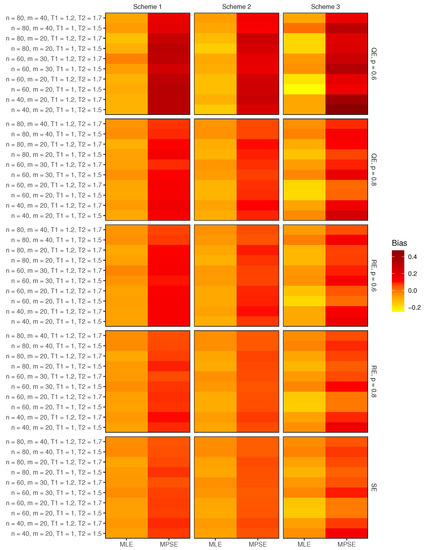
Figure 1. Average biases of the estimators of $S,R_p$ and $Q_q$ for $\lambda =2.5,\theta =2.5$.

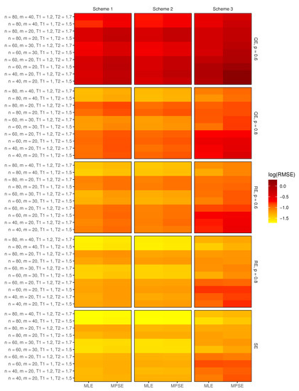
Figure 2. Average $\log ($RMSEs) of the estimators of $S,R_p$ and $Q_q$ for $\lambda =2.5,\theta =2.5$.

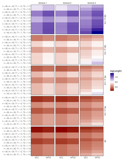
Figure 3. The simulated CILs of ACIs for $S,R_p$ and $Q_q$ when $\lambda =2.5,\theta =2.5$.

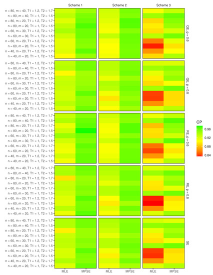
Figure 4. The simulated CPs of ACIs for $S,R_p$ and $Q_q$ when $\lambda =2.5,\theta =2.5$.

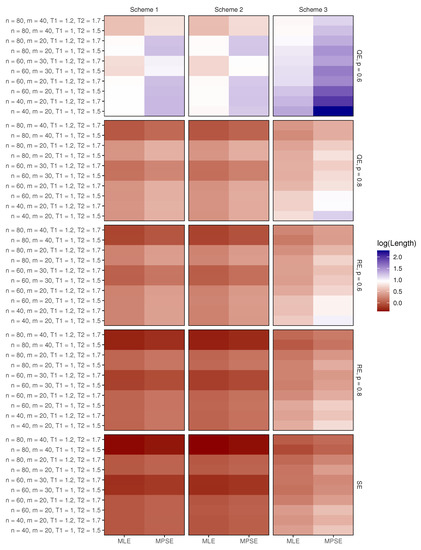
Figure 5. The simulated CILs of PBs for $S,R_p$ and $Q_q$ when $\lambda =2.5,\theta =2.5$.

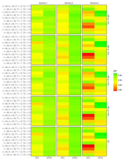
Figure 6. The simulated CPs of PBs for $S,R_p$ and $Q_q$ when $\lambda =2.5,\theta =2.5$.

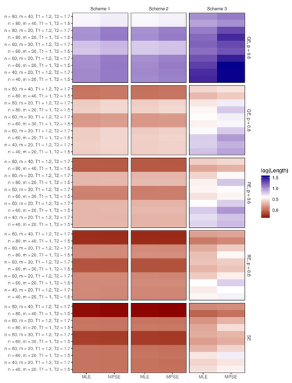
Figure 7. The simulated CILs of SBs for $S,R_p$ and $Q_q$ when $\lambda =2.5,\theta =2.5$.

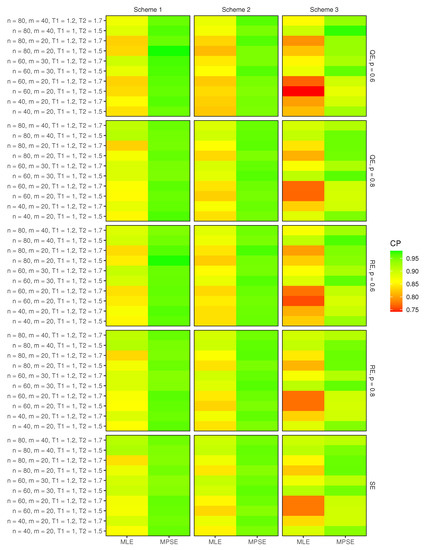
Figure 8. The simulated CPs of SBs for $S,R_p$ and $Q_q$ when $\lambda =2.5,\theta =2.5$.

• Overall, as n (or $m/n$) increases, the estimation efficiency improves, i.e., biases and RMSEs tend to 0, while the CILs decrease for all investigated interval estimates, and their CPs increase as expected.
• As $\theta$ and $\lambda$ increase, both biases and RMSEs of the considered point estimators decrease.
• Estimation based on MLEs underestimates $S,R_p$ and $Q_q$ noticeably, while estimation based on MPSEs overestimates these entropy measurements.
• In most cases, the estimators of the considered entropy measurements based on MLEs outperform their counterparts based on MPSEs in terms of biases and RMSEs. This observation was remarked by [13] when they performed a similar study but based on conventional PT-IIC data.
• Regarding CILs, all considered confidence intervals based on MLEs, are either shorter than their counterparts based on MPSEs or similar.
• Assuming a nominal level of 95%, the least simulated CP among all confidence intervals and simulation settings was 75%. It is observed that confidence intervals based on MPSEs outperformed their counterparts based on MLEs in terms of CPs and sometimes achieved the nominal level. This observation is noticed in all considered simulation settings except for the PBs intervals in the case of Scheme 3 (i.e., IAPT-IIC).

6. Illustrative Examples

In this section, two numerical applications are reported to illustrate the applications of the proposed methodologies to natural phenomena. The first dataset (Data No. 1) consists of the vinyl chloride data (in mg/L) obtained from clean-up-gradient monitoring wells. Several researchers analyzed the data; see Bhaumik et al. [42], Vishwakarma et al. [43], and Okasha and Nassar [13]. The second dataset (referred to as Data No. 2) contains the times (in min) to breakdown of an insulating fluid between 19 electrodes recorded at 34 kV, see Lawless [44]. See Dey and Nassar [45], Elshahhat and Rastogi [46], and Okasha and Nassar [13] for recent applications using these data. Okasha and Nassar [13] checked the fit of the IW distribution to this dataset via the Kolmogorov–Smirnov and Cramér-von Mises goodness-of-fit tests. They concluded that the IW distribution is a suitable for the given two datasets. Table 4 and Table 5 show a PT-IIC sample, an APT-IIC sample, and an IAPT-IIC sample generated from the original datasets, respectively.

Table 4. Generated samples from Data No. 1.

Scheme	n	$\mathit{m},{\mathit{D}}_1,{\mathit{D}}_2$	${\mathit{T}}_1$	${\mathit{T}}_2$	R	Data
PT-IIC	34	17, -, -	∞	∞	$(1\ast 17)$	0.4, 0.4, 0.5, 0.5, 0.6, 0.6, 0.9, 0.9, 1.2,
						1.3, 2.0, 2.4, 2.5, 2.7, 3.2, 4.0, 6.8
APT-IIC	34	17, 8, -	1	∞	$(1\ast 8,0\ast 8,9)$	0.4, 0.4, 0.4, 0.5, 0.6, 0.6, 0.9, 1.0, 1.1,
						1.2, 1.2, 1.3, 1.8, 2.0, 2.0, 2.3, 2.4
IAPT-IIC	34	17, 8, 15	1	2	$(1\ast 8,0\ast 6,11)$	0.4, 0.4, 0.4, 0.5, 0.6, 0.6, 0.9, 1.0, 1.1,
						1.2, 1.2, 1.3, 1.8, 2.0, 2.0

Table 5. Generated samples from Data No. 2.

Scheme	n	$\mathit{m},{\mathit{D}}_1,{\mathit{D}}_2$	${\mathit{T}}_1$	${\mathit{T}}_2$	R	Data
PT-IIC	19	9, -, -	∞	∞	$(1\ast 8,2)$	2.78, 3.16, 4.15, 4.67, 7.35,
						8.01, 12.06, 32.52, 33.91
APT-IIC	19	9, 4, -	30	∞	$(1\ast 4,0\ast 4,6)$	2.78, 3.16, 4.67, 7.35, 31.75,
						32.52, 33.91, 36.71, 72.89
IAPT-IIC	19	9, 4, 7	30	35	$(1\ast 4,0\ast 2,8)$	2.78, 3.16, 4.67, 7.35,
						31.75, 32.52, 33.91

The MLEs and MPSEs of the entropy measures and the corresponding standard errors (SEs) are computed and displayed in Table 6 for the two real datasets. The standard errors are obtained using $B=$ 1000 parametric bootstrap samples. The latter table indicates that if the APT-IIC scheme is considered, then the MLEs should be used to estimate the model parameters. Alternatively, if the IAPT-IIC scheme is utilized, then the MPSEs should be considered when estimating the model parameters. Furthermore, one can conclude that the APT-IIC or IAPT-IIC schemes provide more information for Data No. 1, based on MLEs and MPSEs, respectively. On the contrary, it is seen that the PT-IIC scheme and IAPT-IIC schemes provide more information regarding Data No. 2, using the MLEs and MPSEs, respectively. This analysis shows that the APT-IIC and IAPT-IIC provide more information than the traditional PT-IIC for some progressive censoring plans. Alongside the calculated estimators and corresponding SEs for both datasets, the parametric bootstrap samples are used to calculate the observed lengths of confidence intervals (CIs) for ACIs, PB, and SB confidence intervals of the different entropy measures using 90%, 95%, and 99% confidence levels, as shown in Table 7 and Table 8 for Data No. 1 and No. 2, respectively. The following remarks are observed from the latter tables:

Table 6. The various estimates of entropies (with their SEs in parentheses) for the real data.

		MLE
Data	Entropy	PT-IIC	APT-IIC	IAPT-IIC
1	SE	2.597 (0.452)	2.213 (0.409)	2.253 (0.441)
	RE (0.6)	4.765 (1.369)	3.823 (0.970)	3.924 (1.082)
	QE (0.6)	14.315 (6.678)	9.034 (4.083)	9.512 (4.636)
	RE (0.9)	2.822 (0.505)	2.400 (0.450)	2.445 (0.487)
	QE (0.9)	3.261 (0.618)	2.713 (0.559)	2.770 (0.604)
2	SE	4.664 (0.661)	6.419 (0.900)	6.425 (1.030)
	RE (0.7)	5.881 (1.207)	10.096 (3.655)	10.123 (4.236)
	QE (0.7)	16.126 (1.769)	65.581 (10.360)	66.137 (12.071)
	RE (0.9)	4.913 (0.746)	6.951 (1.103)	6.959 (1.270)
	QE (0.9)	6.344 (0.769)	10.039 (1.140)	10.055 (1.312)
		MPSE
Data	Entropy	PT-IIC	APT-IIC	IAPT-IIC
1	SE	3.194 (0.581)	2.278 (0.491)	1.462 (0.466)
	RE (0.6)	6.704 (3.108)	3.827 (1.143)	2.427 (0.816)
	QE (0.6)	34.021 (22.934)	9.056 (4.501)	4.100 (3.167)
	RE (0.9)	3.483 (0.666)	2.461 (0.540)	1.593 (0.500)
	QE (0.9)	4.166 (0.795)	2.791 (0.664)	1.727 (0.645)
2	SE	4.738 (0.729)	5.967 (0.899)	4.143 (0.784)
	RE (0.7)	6.201 (1.503)	9.185 (3.286)	5.358 (1.474)
	QE (0.7)	18.085 (2.513)	49.104 (8.633)	13.298 (2.474)
	RE (0.9)	5.025 (0.840)	6.460 (1.100)	4.392 (0.889)
	QE (0.9)	6.528 (0.886)	9.080 (1.156)	5.515 (0.959)

Table 7. The observed lengths of CIs for the Data No. 1.

	PT-IIC Scheme
Method	Entropy	90% PB	95% PB	99% PB	90% SB	95% SB	99% SB	90% ACI	95% ACI	99% ACI
MLE	SE	1.518	1.769	2.338	1.630	1.944	2.554	1.488	1.774	2.331
	RE (0.7)	4.663	5.915	8.752	5.029	6.133	8.866	4.503	5.366	7.052
	QE (0.7)	42.955	67.353	186.000	33.999	42.096	55.371	21.968	26.177	34.402
	RE (0.9)	1.746	2.033	2.742	1.914	2.201	2.944	1.661	1.980	2.602
	QE (0.9)	2.301	2.686	3.633	2.504	2.887	3.803	2.033	2.423	3.184
MPSE	SE	1.528	1.823	2.400	1.751	2.094	2.892	1.911	2.277	2.993
	RE (0.7)	8.587	10.095	13.911	9.655	12.035	17.533	10.224	12.183	16.011
	QE (0.7)	359.823	617.294	2256.764	162.740	212.909	327.560	75.445	89.898	118.146
	RE (0.9)	2.026	2.393	3.170	2.098	2.443	3.523	2.190	2.609	3.429
	QE (0.9)	2.952	3.488	4.658	3.025	3.542	5.128	2.615	3.116	4.095
	APT-IIC Scheme
Method	Entropy	90% PB	95% PB	99% PB	90% SB	95% SB	99% SB	90% ACI	95% ACI	99% ACI
MLE	SE	1.326	1.607	2.051	1.438	1.730	2.280	1.345	1.602	2.106
	RE (0.7)	3.363	4.255	5.827	3.451	4.180	5.470	3.192	3.803	4.998
	QE (0.7)	18.232	26.308	49.949	15.298	18.480	24.171	13.431	16.004	21.033
	RE (0.9)	1.439	1.739	2.342	1.575	1.893	2.597	1.479	1.762	2.316
	QE (0.9)	1.818	2.194	2.969	1.980	2.372	3.250	1.837	2.189	2.877
MPSE	SE	1.238	1.471	1.937	1.681	1.984	2.708	1.616	1.925	2.530
	RE (0.7)	2.930	3.563	4.838	4.488	5.424	6.873	3.759	4.479	5.886
	QE (0.7)	13.732	18.080	29.583	19.883	23.782	30.958	14.808	17.645	23.189
	RE (0.9)	1.377	1.616	2.197	1.882	2.226	3.120	1.777	2.117	2.782
	QE (0.9)	1.721	2.021	2.741	2.275	2.780	3.851	2.183	2.602	3.419
	IAPT-IIC Scheme
Method	Entropy	90% PB	95% PB	99% PB	90% SB	95% SB	99% SB	90% ACI	95% ACI	99% ACI
MLE	SE	1.988	2.280	2.825	2.237	2.603	3.176	1.452	1.730	2.273
	RE (0.7)	4.174	5.408	7.830	5.755	6.677	8.889	3.558	4.240	5.572
	QE (0.7)	21.877	35.278	83.559	22.208	26.256	34.681	15.251	18.173	23.883
	RE (0.9)	2.247	2.595	3.179	2.617	3.023	3.546	1.602	1.908	2.508
	QE (0.9)	2.793	3.224	3.999	3.096	3.535	4.094	1.988	2.369	3.113
MPSE	SE	1.177	1.401	1.826	1.789	2.118	2.849	1.532	1.826	2.400
	RE (0.7)	1.847	2.162	2.869	3.553	4.209	5.597	2.685	3.200	4.205
	QE (0.7)	3.903	4.581	6.339	6.514	7.389	8.990	10.419	12.415	16.316
	RE (0.9)	1.236	1.490	1.925	1.937	2.313	3.143	1.644	1.960	2.575
	QE (0.9)	1.384	1.665	2.140	1.999	2.404	3.117	2.123	2.530	3.325

Table 8. The observed lengths of CIs for the Data No. 2.

	PT-IIC Scheme
Method	Entropy	90% PB	95% PB	99% PB	90% SB	95% SB	99% SB	90% ACI	95% ACI	99% ACI
MLE	SE	2.155	2.591	3.640	2.548	3.268	4.760	2.174	2.591	3.405
	RE(0.7)	3.892	4.538	6.173	4.933	6.297	9.497	3.970	4.731	6.218
	QE(0.7)	24.058	29.552	44.329	35.504	55.800	109.868	5.821	6.936	9.116
	RE(0.9)	2.399	3.010	4.194	2.951	3.899	5.457	2.454	2.924	3.843
	QE(0.9)	3.857	4.842	6.707	5.068	6.822	9.784	2.530	3.015	3.963
MPSE	SE	2.331	2.796	3.645	2.454	3.026	3.977	2.397	2.856	3.753
	RE(0.7)	5.706	7.061	14.586	4.990	6.168	8.271	4.945	5.892	7.744
	QE(0.7)	53.727	77.886	746.232	32.066	43.943	66.353	8.266	9.850	12.945
	RE(0.9)	2.733	3.281	4.404	2.816	3.503	4.843	2.763	3.292	4.327
	QE(0.9)	4.564	5.512	7.535	4.714	6.183	9.169	2.915	3.474	4.565
	APT-IIC Scheme
Method	Entropy	90% PB	95% PB	99% PB	90% SB	95% SB	99% SB	90% ACI	95% ACI	99% ACI
MLE	SE	2.804	3.349	4.313	3.440	4.137	6.141	2.960	3.527	4.636
	RE(0.7)	8.978	11.326	14.857	16.522	22.075	37.542	12.024	14.327	18.829
	QE(0.7)	266.041	477.384	1085.660	475.609	664.807	1561.745	34.080	40.609	53.369
	RE(0.9)	3.683	4.304	5.727	4.529	5.315	7.657	3.628	4.323	5.681
	QE(0.9)	7.333	8.663	11.661	9.071	10.922	16.283	3.749	4.467	5.870
MPSE	SE	2.604	3.175	4.099	3.493	4.322	5.968	2.958	3.525	4.632
	RE(0.7)	8.232	10.790	14.285	17.378	22.106	29.118	10.809	12.880	16.927
	QE(0.7)	154.209	311.100	725.601	358.010	449.731	903.188	28.400	33.841	44.474
	RE(0.9)	3.144	4.009	5.012	4.358	5.395	7.132	3.619	4.313	5.668
	QE(0.9)	5.667	7.374	9.291	8.243	10.021	13.872	3.803	4.531	5.955
	IAPT-IIC Scheme
Method	Entropy	90% PB	95% PB	99% PB	90% SB	95% SB	99% SB	90% ACI	95% ACI	99% ACI
MLE	SE	4.192	4.904	6.868	4.615	5.490	7.508	3.389	4.039	5.308
	RE(0.7)	9.067	11.251	16.179	25.806	33.358	43.823	13.935	16.605	21.822
	QE(0.7)	212.786	372.576	1351.513	782.050	1174.103	1973.134	39.711	47.319	62.187
	RE(0.9)	6.442	7.626	11.217	5.965	6.927	9.608	4.177	4.978	6.542
	QE(0.9)	14.273	17.609	29.263	12.933	14.969	22.750	4.316	5.143	6.759
MPSE	SE	2.212	2.667	3.516	3.534	4.216	5.726	2.579	3.073	4.039
	RE(0.7)	3.723	4.654	5.935	8.070	9.603	11.600	4.848	5.776	7.591
	QE(0.7)	14.064	19.150	27.711	47.129	60.478	114.477	8.139	9.698	12.746
	RE(0.9)	2.409	2.872	3.977	4.144	4.973	7.261	2.924	3.484	4.579
	QE(0.9)	3.375	4.052	5.524	6.495	8.420	12.419	3.156	3.760	4.942

• As the confidence level increases, the lengths of the CIs increase as expected.
• The CIs obtained based on APT-IIC and IAPT-IIC have fewer lengths than those obtained using the PT-IIC scheme.
• The bootstrap-based confidence intervals based on MPSEs have fewer lengths than those obtained using their counterparts established based on the MLEs.

Combining the above results, we suggest using the APT-IIC or IAPT-IIC schemes to study the IW distribution characteristics. Furthermore, one can decide which scheme to use based on the MLEs or MPSEs using the smallest SEs calculated from bootstrap samples.

7. Conclusions

This paper has considered two estimation methods for Rényi, q, and Shannon entropies for inverse Weibull distribution based on improved adaptive progressively Type-II censored data. The estimation procedures of interest are the methods of maximum likelihood and maximum product of spacing. The point estimators are obtained through the invariance property. Moreover, the asymptotic confidence intervals and bootstrapped-based confidence intervals are also computed. Monte Carlo simulations have been carried out to examine estimation efficiency for the considered inferential procedures. Furthermore, two illustrative examples have been analyzed for the same purpose. The numerical study demonstrates that the maximum likelihood method yields reasonable point estimates for the three entropy measurements. On the other hand, numerical outcomes suggest that the maximum product of the spacing method is preferred when obtaining confidence intervals for these measurements. The data analysis demonstrated that the samples obtained using improved adaptive progressive Type-II or adaptive progressive Type-II censoring schemes provided more information than those gathered based on the traditional progressive Type-II censoring scheme based on the used progressive censoring plans.

Two research directions are being considered in the future. One research direction is to compare the performance of the considered conventional estimation methods to other non-conventional counterparts, such as those established on the least squares theory. Another research direction that needs to be addressed is comparing estimation efficiency between improved adaptive progressively Type-II censored data and generalized progressively hybrid censored data.

References

- Shannon, C.E. A Mathematical Theory of Communication. Bell Syst. Tech. J. 1948, 27, 379–423. [Google Scholar] [CrossRef]
- Amigó, J.; Balogh, S.; Hernández, S. A Brief Review of Generalized Entropies. Entropy 2018, 20, 813. [Google Scholar] [CrossRef]
- Rényi, A. On measures of entropy and information. In Proceedings of the Fourth Berkeley Symposium on Mathematical Statistics and Probability, Berkeley, CA, USA, 20 June–30 July 1961; University of California Press: Berkeley, CA, USA, 1961; pp. 547–561. [Google Scholar]
- Tsallis, C. Possible generalization of Boltzmann-Gibbs statistics. J. Stat. Phys. 1988, 52, 479–487. [Google Scholar] [CrossRef]
- Wong, K.; Chen, S. The entropy of ordered sequences and order statistics. IEEE Trans. Inf. Theory 1990, 36, 276–284. [Google Scholar] [CrossRef]
- Baratpour, S.; Ahmadi, J.; Arghami, N.R. Entropy properties of record statistics. Stat. Pap. 2007, 48, 197–213. [Google Scholar] [CrossRef]
- Morabbi, H.; Razmkhah, M. Entropy of Hybrid Censoring Schemes. J. Stat. Res. Iran 2010, 6, 161–176. [Google Scholar] [CrossRef]
- Abo-Eleneen, Z.A. The Entropy of Progressively Censored Samples. Entropy 2011, 13, 437–449. [Google Scholar] [CrossRef]
- Cramer, E.; Bagh, C. Minimum and Maximum Information Censoring Plans in Progressive Censoring. Commun. Stat.-Theory Methods 2011, 40, 2511–2527. [Google Scholar] [CrossRef]
- Cho, Y.; Sun, H.; Lee, K. An Estimation of the Entropy for a Rayleigh Distribution Based on Doubly-Generalized Type-II Hybrid Censored Samples. Entropy 2014, 16, 3655–3669. [Google Scholar] [CrossRef]
- Hassan, A.S.; Zaky, A.N. Estimation of entropy for inverse Weibull distribution under multiple censored data. J. Taibah Univ. Sci. 2019, 13, 331–337. [Google Scholar] [CrossRef]
- Bantan, R.A.R.; Elgarhy, M.; Chesneau, C.; Jamal, F. Estimation of Entropy for Inverse Lomax Distribution under Multiple Censored Data. Entropy 2020, 22, 601. [Google Scholar] [CrossRef] [PubMed]
- Okasha, H.; Nassar, M. Product of spacing estimation of entropy for inverse Weibull distribution under progressive type-II censored data with applications. J. Taibah Univ. Sci. 2022, 16, 259–269. [Google Scholar] [CrossRef]
- Keller, A.; Goblin, M.; Farnworth, N. Reliability analysis of commercial vehicle engines. Reliab. Eng. 1985, 10, 15–25. [Google Scholar] [CrossRef]
- Calabria, R.; Pulcini, G. Bayes 2-sample prediction for the inverse weibull distribution. Commun. Stat.-Theory Methods 1994, 23, 1811–1824. [Google Scholar] [CrossRef]
- Jiang, R.; Murthy, D.; Ji, P. Models involving two inverse Weibull distributions. Reliab. Eng. Syst. Saf. 2001, 73, 73–81. [Google Scholar] [CrossRef]
- Mahmoud, M.; Sultan, K.; Amer, S. Order statistics from inverse weibull distribution and associated inference. Comput. Stat. Data Anal. 2003, 42, 149–163. [Google Scholar] [CrossRef]
- Sultan, K.S. Bayesian Estimates Based on Record Values from the Inverse Weibull Lifetime Model. Qual. Technol. Quant. Manag. 2008, 5, 363–374. [Google Scholar] [CrossRef]
- Kundu, D.; Howlader, H. Bayesian inference and prediction of the inverse Weibull distribution for Type-II censored data. Comput. Stat. Data Anal. 2010, 54, 1547–1558. [Google Scholar] [CrossRef]
- Hassan, A.S.; Assar, S.M.; Zaky, A.N. Constant-stress partially accelerated life tests for inverted Weibull distribution with multiple censored data. Int. J. Adv. Stat. Probab. 2015, 3, 72. [Google Scholar] [CrossRef]
- Kumar, K.; Kumar, I. Estimation in Inverse Weibull Distribution Based on Randomly Censored Data. Statistica 2019, 79, 47–74. [Google Scholar] [CrossRef]
- Al-Duais, F.S. Bayesian Analysis of Record Statistic from the Inverse Weibull Distribution under Balanced Loss Function. Math. Probl. Eng. 2021, 2021, 6648462. [Google Scholar] [CrossRef]
- Rastogi, M.K.; Tripathi, Y.M.; Wu, S.J. Estimating the parameters of a bathtub-shaped distribution under progressive type-II censoring. J. Appl. Stat. 2012, 39, 2389–2411. [Google Scholar] [CrossRef]
- Ahmed, E.A. Bayesian estimation based on progressive Type-II censoring from two-parameter bathtub-shaped lifetime model: An Markov chain Monte Carlo approach. J. Appl. Stat. 2013, 41, 752–768. [Google Scholar] [CrossRef]
- Dey, S.; Nassar, M.; Maurya, R.K.; Tripathi, Y.M. Estimation and prediction of Marshall–Olkin extended exponential distribution under progressively type-II censored data. J. Stat. Comput. Simul. 2018, 88, 2287–2308. [Google Scholar] [CrossRef]
- Balakrishnan, N.; Aggarwala, R. Progressive Censoring; Birkhäuser: Boston, MA, USA, 2000. [Google Scholar] [CrossRef]
- Balakrishnan, N.; Cramer, E. The Art of Progressive Censoring; Springer: New York, NY, USA, 2014. [Google Scholar] [CrossRef]
- Dey, S.; Nassar, M.; Kumar, D. Moments and estimation of reduced Kies distribution based on progressive type-II right censored order statistics. Hacet. J. Math. Stat. 2018, 48, 332–350. [Google Scholar] [CrossRef]
- Kumar, D.; Nassar, M.; Malik, M.R.; Dey, S. Estimation of the Location and Scale Parameters of Generalized Pareto Distribution Based on Progressively Type-II Censored Order Statistics. Ann. Data Sci. 2023, 10, 349–383. [Google Scholar] [CrossRef]
- Ng, H.K.T.; Kundu, D.; Chan, P.S. Statistical analysis of exponential lifetimes under an adaptive Type-II progressive censoring scheme. Nav. Res. Logist. (NRL) 2009, 56, 687–698. [Google Scholar] [CrossRef]
- Ye, Z.S.; Chan, P.S.; Xie, M.; Ng, H.K.T. Statistical inference for the extreme value distribution under adaptive Type-II progressive censoring schemes. J. Stat. Comput. Simul. 2014, 84, 1099–1114. [Google Scholar] [CrossRef]
- Sobhi, M.M.A.; Soliman, A.A. Estimation for the exponentiated Weibull model with adaptive Type-II progressive censored schemes. Appl. Math. Model. 2016, 40, 1180–1192. [Google Scholar] [CrossRef]
- EL-Sagheer, R.M.; Mahmoud, M.A.W.; Abdallah, S.H.M. Statistical inferences for new Weibull-Pareto distribution under an adaptive Type-II progressive censored data. J. Stat. Manag. Syst. 2018, 21, 1021–1057. [Google Scholar] [CrossRef]
- Yan, W.; Li, P.; Yu, Y. Statistical inference for the reliability of Burr-XII distribution under improved adaptive Type-II progressive censoring. Appl. Math. Model. 2021, 95, 38–52. [Google Scholar] [CrossRef]
- Cheng, R.C.H.; Amin, N.A.K. Estimating Parameters in Continuous Univariate Distributions with a Shifted Origin. J. R. Stat. Soc. Ser. B (Methodol.) 1983, 45, 394–403. [Google Scholar] [CrossRef]
- Coolen, F.; Newby, M. A Note on the Use of the Product of Spacings in Bayesian Inference; Memorandum COSOR, Technische Universiteit Eindhoven: Eindhoven, The Netherlands, 1990. [Google Scholar]
- Anatolyev, S.; Kosenok, G. An Alternative to Maximum Likelihood Based on Spacings. Econom. Theory 2005, 21, 472–476. [Google Scholar] [CrossRef]
- Efron, B. The Jackknife, the Bootstrap and Other Resampling Plans; Society for Industrial and Applied Mathematics: Philadelphia, PA, USA, 1982. [Google Scholar] [CrossRef]
- Hall, P. Theoretical Comparison of Bootstrap Confidence Intervals. Ann. Stat. 1988, 16, 927–953. [Google Scholar] [CrossRef]
- Balakrishnan, N.; Sandhu, R.A. A Simple Simulational Algorithm for Generating Progressive Type-II Censored Samples. Am. Stat. 1995, 49, 229–230. [Google Scholar] [CrossRef]
- R Core Team. R: A Language and Environment for Statistical Computing; R Foundation for Statistical Computing: Vienna, Austria, 2022. [Google Scholar]
- Bhaumik, D.K.; Kapur, K.; Gibbons, R.D. Testing Parameters of a Gamma Distribution for Small Samples. Technometrics 2009, 51, 326–334. [Google Scholar] [CrossRef]
- Vishwakarma, P.K.; Kaushik, A.; Pandey, A.; Singh, U.; Singh, S.K. Bayesian Estimation for Inverse Weibull Distribution Under Progressive Type-II Censored Data With Beta-Binomial Removals. Austrian J. Stat. 2018, 47, 77–94. [Google Scholar] [CrossRef]
- Lawless, J.F. Statistical Models and Methods for Lifetime Data; Wiley-Interscience: Hoboken, NJ, USA, 2003; p. 630. [Google Scholar]
- Dey, S.; Nassar, M. Classical methods of estimation on constant stress accelerated life tests under exponentiated Lindley distribution. J. Appl. Stat. 2019, 47, 975–996. [Google Scholar] [CrossRef]
- Elshahhat, A.; Rastogi, M.K. Estimation of Parameters of Life for an Inverted Nadarajah–Haghighi Distribution from Type-II Progressively Censored Samples. J. Indian Soc. Probab. Stat. 2021, 22, 113–154. [Google Scholar] [CrossRef]
Disclaimer/Publisher’s Note: The statements, opinions and data contained in all publications are solely those of the individual author(s) and contributor(s) and not of MDPI and/or the editor(s). MDPI and/or the editor(s) disclaim responsibility for any injury to people or property resulting from any ideas, methods, instructions or products referred to in the content. |
© 2023 by the authors. Licensee MDPI, Basel, Switzerland. This article is an open access article distributed under the terms and conditions of the Creative Commons Attribution (CC BY) license (https://creativecommons.org/licenses/by/4.0/).