A Clustering-Based Approach to Detecting Critical Traffic Road Segments in Urban Areas

Abstract

This paper introduces a parameter-free clustering-based approach to detecting critical traffic road segments in urban areas, i.e., road segments of spatially prolonged and high traffic accident risk. In addition, it proposes a novel domain-specific criterion for evaluating the clustering results, which promotes the stability of the clustering results through time and inter-period accident spatial collocation, and penalizes the size of the selected clusters. To illustrate the proposed approach, it is applied to data on traffic accidents with injuries or death that occurred in three of the largest cities of Serbia over the three-year period.

1. Introduction

Clustering has an important role in road traffic data analysis. Two research lines currently receive the most attention in the field. The first line is related to traffic logistics, e.g., traffic load and congestion analysis, and vehicle routing. The second line is related to traffic safety, e.g., traffic accident pattern detection, hotspot detection and critical road segment detection. Some recent studies that employ clustering in the context of traffic analysis are summarized in

Table 1. Summary of some recent studies that employ clustering in the context of traffic safety.

Ref.	Task	Clustering Approach
[1]	traffic load analysis	improved k-means clustering algorithm
[2]	traffic congestion analysis	self-organizing maps neural network
[3]	traffic state classification	k-medoids algorithm
[4]	road network level identification	k-means algorithm
[5]	traffic congestion analysis	grey relational clustering model
[6]	traffic accidents and pattern extraction	ROCK algorithm
[7]	traffic accident pattern identification	COOLCAT algorithm
[8]	traffic accident factor analysis	k-means algorithm
[9]	road traffic accident modeling	a comparative study of machine learning classifiers
[10]	traffic accident black spots identification	HDBSCAN algorithm
[11]	traffic congestion analysis	k-means algorithm
[12]	driving behavior risk analysis	k-means algorithm
[13]	optimal path routing	a modified K-medoids algorithm
[14]	analysis of pedestrian crash fatalities and severe injuries	KDE method
[15]	traffic-management system	DBSCAN agorithm
[16]	severity of traffic accident analysis	DBSCAN algorithm
[17]	highway safety assessment	k-means algorithm
[18]	pedestrian crash severity analysis	KDE method
[19]	detection of road segments of spatially prolonged and high traffic accident risk	a clustering algorithm based on the Gestalt principle of proximity

.

This paper goes along the second research line. It introduces a parameter-free approach to clustering critical traffic road segments in urban areas, i.e., road segments of spatially prolonged and high traffic accident risk. With this respect, we build on and extend the specific approach introduced in [19]. Two traffic accidents are considered related (i.e., as belonging to the same cluster) if the spatial distance between them is less than or equal to a predefined threshold value $\widehat{\tau }$, i.e.,

$$a_i\sim a_j\iff d(a_i,a_j)\le \widehat{\tau }.$$

(1)

A road segment is considered to be at spatially prolonged traffic accident risk if it is associated with a set of traffic accidents $A=\{a_1,a_2,\dots ,a_n\}$ in a given period such that the transitive closure of relation (1) over set A provides a connected graph. A road segment is considered to be at high traffic accident risk when it is associated with a significant number of accidents when compared to other road segments in the given area. In the first phase of the algorithm, clusters are determined by the transitive closure of relation (1), which can be described as follows. Let $\mathcal{A}$ be a set of traffic accidents, each of which is described only by its positional coordinates. At the start of the algorithm, each accident $a_i\in \mathcal{A}$ is assigned to a separate cluster $k\left(a_i\right)$. In addition, let $\mathcal{X}(\mathcal{A},\widehat{\tau })$ be a sequence of all combinations of two traffic accidents whose distance is less than or equal to $\widehat{\tau }$. This sequence is ordered by non-decreasing distance between traffic accidents:

$$\mathcal{X}(\mathcal{A},\widehat{\tau })=\left(a_{11}{a}_{12}\right),\left(a_{21}{a}_{22}\right),\dots ,\left(a_{n1}{a}_{n2}\right),$$

(2)

where

$$(\forall 1\le i\le n)(\{a_{i1},a_{i2}\}\subset \mathcal{A}\wedge d(a_{i1},a_{i2})<\widehat{\tau }\wedge i<j\iff d(a_{i1},a_{i2})\le d(a_{j1},a_{j2})).$$

(3)

Sequence $\mathcal{X}(\mathcal{A},\widehat{\tau })$ is iterated from the first to the last ordered pair. For each pair $(a_{i_1},a_{i_2})$, clusters $k\left(a_{i_1}\right)$ and $k\left(a_{i_2}\right)$ are merged, i.e.,

$$\begin{array}{cc}\hfill & foreach(a_{i_1},a_{i_2})\in \mathcal{X}(\mathcal{A},\tau )\hfill \\ \hfill & ifk\left(a_{i_1}\right)\ne k\left(a_{i_2}\right)then\hfill \\ \hfill & mergeclustersk\left(a_{i_1}\right)andk\left(a_{i_2}\right)\hfill \end{array}$$

(4)

In other words, the clusters are merged in a bottom–up manner. In the second phase, the clusters that are dominant in terms of number of accidents are selected as critical. This phase represents an adaptation of the method of threshold selection for image binarization introduced in [20] (pp. 120–121).

It should be noted that the spatial threshold $\widehat{\tau }$ was applied as an input hyperparameter to this algorithm. However, in the general case, its optimal value should be adaptively derived depending on a given traffic area. The contribution of this study can be summarized as follows:

• We introduce an approach to automatic threshold value estimation based on knee-point detection. In general, a knee point in considered the operational point at which the system achieves the trade-off between cost and performance dependent on a tunable parameter. Thus, the traffic accident data are clustered repetitively by varying threshold value $\widehat{\tau }$, and the operational threshold value is selected with respect to the introduced internal evaluation measure. Various knee-point detection algorithms have already been applied to determine the optimal number of clusters, cf. [21,22,23]. However, the criteria for the evaluation of clustering results are usually defined in a domain-independent manner, e.g., based on the within-cluster dispersion, between-cluster dispersion, etc. In contrast to those approaches, this paper proposes a novel domain-specific criterion for evaluating the clustering results, which promotes the stability of clustering results through time and inter-period accident spatial collocation, and penalizes the size of selected clusters.
• We propose an adaptation of the Kneedle algorithm [24] aimed at the automatic determination of the operational threshold value.
• In our approach, an urban area (e.g., a city) encompasses a set of possibly diverse administrative units (e.g., municipalities), each of which exercises traffic control jurisdiction over its roads. Thus, the criteria for the determination of critical road segments may differ among different administrative units. One of the novelties of the proposed approach is that traffic analysis is conducted for each administrative unit separately, but the clustering results are evaluated at the level of the entire urban area.
• For the purpose of illustration, the proposed approach is applied to data on traffic accidents with injuries or death that occurred in three of the largest cities of Serbia over the three-year period [25,26,27], as summarized in

  Table 2. Traffic accidents with injuries or death.

  City	2019	2020	2021	Total
  Beograd	4684	3720	4072	12,476
  Novi Sad	1710	1464	1574	4748
  Niš	607	521	528	1656
  Total	7001	5705	6174	18,880

  . For each accident, only its unique identification number and positional coordinates are taken into account. In an external validation, the obtained clustering results are positively evaluated with respect to the locations of traffic cameras.

The rest of this paper is structured as follows. Section 2 introduces an evaluation measure for traffic accident clustering. Section 3 proposes an adaptation of the Kneedle algorithm. Section 4 and Section 5 present the results and evaluation of the proposed approach. Section 6 concludes the paper.

2. Evaluation Measure for Traffic Accident Clustering

This section introduces an evaluation measure for traffic accident clustering based on three separate but related submeasures:

• Stability of clustering results through time;
• Inter-period accident spatial collocation;
• Area covered by the selected clusters.

2.1. Stability of Clustering Results through Time

To estimate the stability of clustering results through time, the clustering algorithm is applied to data on traffic accidents collected in the same spatial areas over two different periods, which we denote as $P_1$ and $P_2$, respectively, where $P_1$ precedes $P_2$.

Without loss of generality, let us assume that a city has n municipalities, represented by the vector:

$$M=m_1,m_2,\dots ,m_n.$$

(5)

The clustering algorithm is applied separately for each municipality. For the given threshold value ${\tau }_j$ and municipality $m_i$, the following steps are performed:

1.

The clustering algorithm [19] is applied to data on traffic accidents that occurred in municipality $m_i$ over period $P_1$.

2.

We calculate the shares (i.e., percentage) of all traffic accidents that occurred in municipality $m_i$ over period $P_1$ and $P_2$, respectively, that belong to the clusters selected in Step 1. We denote these shares as $s_1(m_i,{\tau }_j,P_1)$ and $s_2(m_i,{\tau }_j,P_2)$.

Example 1.

Let us adopt the following input parameter settings:

• The municipality of Zvezdara (denoted as m);
• Threshold value $\tau =170m$;
• Period $P_1$ runs from January 2019 to December 2020;
• Period $P_2$ runs from January 2021 to December 2021.

The execution of the above algorithm for the adopted parameter settings can be summarized as follows:

1. 

Over period $P_1$, 631 traffic accidents with injuries or death occurred in the municipality of Zvezdara. Figure 1a shows a map of all these traffic accidents. When the clustering algorithm is applied on this set of traffic accidents, four clusters are obtained, as shown in Figure 1b.

2. 

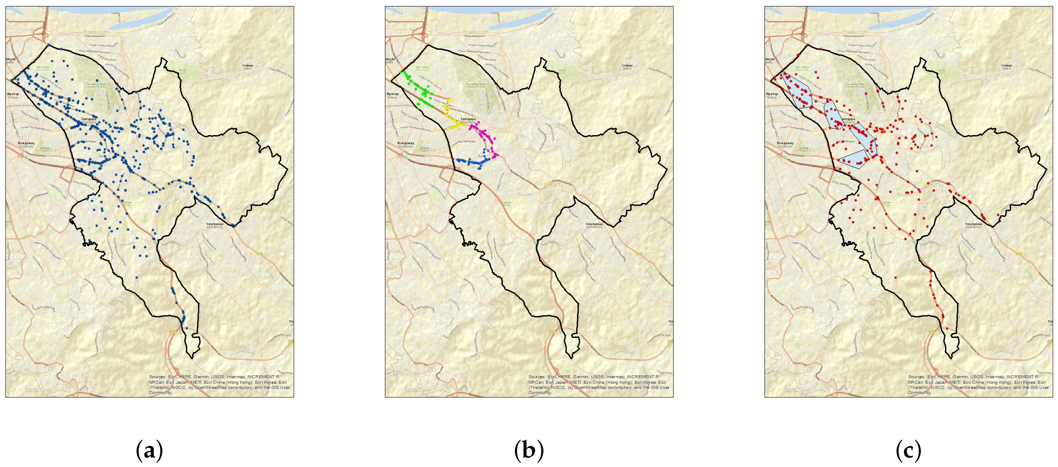
The four selected clusters contain 257 traffic accidents. Thus, the share of the traffic accidents that occurred in the municipality over period $P_1$ that belong to the selected clusters is

$$s_1(m,\tau ,P_1)={\displaystyle \frac{257}{631}}=40.729\%.$$

(6)

3. 

Over period $P_2$, 317 traffic accidents with injuries or death occurred in the municipality of Zvezdara. Figure 1c shows a map of all these traffic accidents. In addition, each of the clusters given in Figure 1a is represented as the minimum bounding box of its convex hull in Figure 1c. The number of accidents occurred over this period that belong to the areas covered by the clusters selected in Step 1 is 131. The share of the captured traffic accidents is

$$s_2(m,\tau ,P_2)={\displaystyle \frac{131}{317}}=41.325\%.$$

(7)

When this sequence of steps is performed for all municipalities in set M, the result can be represented by two vectors:

$$\begin{array}{cc}\hfill S_1(M,{\tau }_j,P_1)& =s_1(m_1,{\tau }_j,P_1),s_1(m_2,{\tau }_j,P_1),\dots ,s_1(m_n,{\tau }_j,P_1),\hfill \\ \hfill S_2(M,{\tau }_j,P_2)& =s_2(m_1,{\tau }_j,P_2),s_2(m_2,{\tau }_j,P_2),\dots ,s_2(m_n,{\tau }_j,P_2).\hfill \end{array}$$

(8)

In general, municipalities in a city may differ in area, the number of inhabitants, traffic density and other various factors. However, we consider them as being equally important in estimating the stability of clustering results through time. Therefore, for a given threshold value ${\tau }_j$, the stability of clustering results through time is estimated as the cosine similarity between the vectors in Equation (8):

$$s(M,{\tau }_j,P_1,P_2)={\displaystyle \frac{{\displaystyle \sum _{k=1}^n}(s_1(m_k,{\tau }_j,P_1)·s_2(m_k,{\tau }_j,P_2))}{\sqrt{{\displaystyle \sum _{k=1}^n}{s}_1^2(m_k,{\tau }_j,P_1)}·\sqrt{{\displaystyle \sum _{k=1}^n}{s}_2^2(m_k,{\tau }_j,P_2)}}}.$$

(9)

Since all elements of the vectors in Equation (8) are positive, value $s(M,{\tau }_j,P_1,P_2)$ is always in range $[0,1]$, where value 1 represents the maximum stability (i.e., the maximum similarity between the vectors), and 0 represents the minimum stability.

Example 2.

We keep the following subset of input parameters adopted in Example 1 and estimate the stability of the clustering results for the city of Belgrade. The results obtained when the above algorithm is applied to traffic accident data collected in all municipalities over periods $P_1$ and $P_2$ are given in

Table 3. Estimating the stability of clustering results through time. The algorithm is applied to traffic accident data collected in Belgrade over periods $P_1$ and $P_2$ and for the arbitrarily selected threshold value $\widehat{\tau }=170\mathrm{m}$. All decimal numbers are rounded to three decimal places.

Municipality	${\mathit{P}}_1=[2019\sim 2020]$			${\mathit{P}}_2=\left[2021\right]$
	# Accidents	# Selected Accidents	Share [%] ${\mathit{s}}_1({\mathit{m}}_1,{\mathit{\tau }}_{\mathit{j}})$	# Accidents	# Selected Accidents	Share [%] ${\mathit{s}}_2({\mathit{m}}_1,{\mathit{\tau }}_{\mathit{j}})$
Barajevo	123	54	43.902	51	21	41.176
Grocka	295	105	35.593	150	40	26.667
Lazarevac	281	98	34.875	123	31	25.203
Mladenovac	206	59	28.641	113	30	26.549
Novi beograd	1126	401	35.613	537	186	34.637
Obrenovac	376	129	34.309	220	59	26.818
Palilula	962	308	32.017	384	132	34.375
Rakovica	297	105	35.354	141	44	31.206
Savski venac	572	311	54.371	270	155	57.407
Sopot	100	28	28.000	49	10	20.408
Stari grad	316	263	83.228	176	145	82.386
Surčin	231	86	37.229	125	30	24.000
Voždovac	879	324	36.860	447	177	39.597
Vračar	412	272	66.019	182	139	76.374
Zemun	800	257	32.125	393	126	32.061
Zvezdara	631	257	40.729	317	131	41.325
Čukarica	797	258	32.371	394	132	33.503
Total	8404	3315	39.446	4072	1588	38.998

. The particular elements of vectors $S_1(M,{\tau }_j,P_1)$ and $S_2(M,{\tau }_j,P_2)$ defined in Equation (8) are given in the fourth and seventh columns of the table. Following Equation (9), the stability of clustering results for the adopted parameter settings is estimated as

$$s(M,\tau ,P_1,P_2)=0.990.$$

(10)

2.2. Inter-Period Accident Spatial Collocation

We define the city-level inter-period accident spatial collocation index as the share (i.e., percentage) of all traffic accidents that occurred in city M over period $P_2$ that belong to the areas covered by the clusters obtained when the clustering algorithm was applied to the set of all traffic accidents with injuries or death occurred in M over period $P_1$. This index is denoted as $c(M,{\tau }_j,P_1,P_2)$.

Example 3.

In the last row of Table 3, the following can be observed:

• The total number of accidents with injuries or death over period $P_2$ is 4072.
• The number of accidents that occurred over this period that belong to the areas covered by the clusters obtained when the clustering algorithm was applied to the set of all traffic accidents with injuries or death occurred over period $P_1$ is 1588.

The resulting inter-period accident spatial collocation is

$$c(M,\tau ,P_1,P_2)={\displaystyle \frac{1588}{4072}}=38.998\%.$$

(11)

2.3. Relative Size of Selected Clusters

In our approach, the area covered by a cluster of traffic accidents is conceptualized as the area of the minimum bounding box of its convex hull (cf. Figure 1c). In line with this conceptualization, we define the relative size of selected clusters as the share of the area of city M covered by the clusters obtained when the clustering algorithm is separately applied to sets of traffic accidents occurred in all municipalities of M over period $P_1$. The city-level relative cluster size is denoted as $r(M,{\tau }_j,P_1)$.

Example 4.

Adopting the same input parameter settings as in Example 2, for each municipality,

Table 4. Relative sizes of all selected clusters in Belgrade over period $P_1$ and for the arbitrarily selected threshold value $\widehat{\tau }=170\mathrm{m}$. All decimal numbers are rounded to three decimal places.

Municipality	# Selected Clusters	Area of Selected Clusters [km${}^2$]	Municipality Area [km${}^2$]	Relative Cluster Size [%]
Barajevo	19	0.011	212.831	0.005%
Grocka	22	0.072	299.349	0.024%
Lazarevac	21	0.123	382.540	0.032%
Mladenovac	9	0.151	338.764	0.045%
Novi Beograd	1	7.057	40.756	17.316%
Obrenovac	3	0.644	409.588	0.157%
Palilula	2	4.563	450.351	1.013%
Rakovica	7	0.222	30.025	0.739%
Savski venac	2	2.321	14.082	16.484%
Sopot	11	0.003	270.506	0.001%
Stari grad	1	2.232	5.376	41.527%
Surčin	20	0.053	288.303	0.018%
Voždovac	3	2.233	148.409	1.505%
Vračar	1	2.424	2.911	83.256%
Zemun	8	1.500	149.682	1.002%
Zvezdara	4	1.612	31.087	5.186%
Čukarica	6	1.280	156.909	0.815%
Total	140	26.502	3231.469	0.820%

provides the number of the selected clusters, the area covered by the selected clusters, the area of the municipality and the municipality-level relative size of the selected clusters. The resulting city-level relative size of selected clusters can be derived from the data given in the last row of Table 4:

$$r(M,\tau ,P_1)={\displaystyle \frac{26.502}{3231.469}}=0.820\%.$$

(12)

2.4. Integrated Measure for Traffic Accident Clustering

The clustering algorithm introduced in [19] is designed to automatically detect and select critical road segments, intended for application in circumstances of limited human or technical resources for traffic monitoring and management. In line with this, we introduce an integrated measure for traffic accident clustering that promotes the stability of clustering results and inter-period accident spatial collocation index, and penalize the size of selected clusters, i.e., for given city M, threshold value ${\tau }_j$ and periods $P_1$ and $P_2$, the integrated measure is defined as

$$\eta (M,{\tau }_j,P_1,P_2)={\displaystyle \frac{s(M,{\tau }_j,P_1,P_2)·c(M,{\tau }_j,P_1,P_2)}{r(M,{\tau }_j,P_1,P_2)}},$$

(13)

where we have the following:

• $s(M,{\tau }_j,P_1,P_2)$ represents the stability of the clustering results;
• $c(M,{\tau }_j,P_1,P_2)$ represents the inter-period accident spatial collocation index;
• $r(M,{\tau }_j,P_1,P_2)$ represents the city-level relative size of selected clusters.

Example 5.

Taking (10)–(12) into account, we can calculate the value of the introduced integrated measure:

$$\eta (M,\tau ,P_1,P_2)=47.082.$$

(14)

3. Threshold Selection

For given city M and periods $P_1$ and $P_2$, the integrated measure for traffic accident clustering introduced in the previous section can be considered a function with one input parameter—the threshold value, i.e., $\eta \left(\tau \right)$. This reduction allows for applying the clustering algorithm introduced in [19] repetitively on traffic accidents occurred in city M over periods $P_1$ and $P_2$ by varying its input threshold value $\tau$. This section introduces an algorithm for the selection of an operational threshold value based on the integrated measure defined in Equation (13).

In our approach, the operating threshold value is indicated by a knee point of the plot of the integrated measure $\eta \left(\tau \right)$ versus the applied threshold value $\tau$. Thus, we present an approach for knee point detection. Let $\widehat{\mathcal{D}}$ be a dataset containing n observations for which a knee point should be detected:

$$\widehat{\mathcal{D}}=\left\{({\widehat{\tau }}_i,{\widehat{\eta }}_i)\right|1\le i\le n\wedge {\widehat{\tau }}_i\ge 0\wedge {\widehat{\eta }}_i\ge 0\},$$

(15)

where ${\widehat{\tau }}_i$ represents a threshold value, ${\widehat{\eta }}_i$ represents the integrated measure value obtained for ${\widehat{\tau }}_i$, and threshold values ${\widehat{\tau }}_i$ are evenly spaced, i.e.,

$$(\exists t\in \mathbf{R},t>0)(\forall 1\le i<n)({\widehat{\tau }}_{i+1}-{\widehat{\tau }}_i=t).$$

(16)

First, values ${\widehat{\tau }}_i$ and ${\widehat{\eta }}_i$ are normalized to range $[0,1]$ without changing the distribution of the data [24], i.e.,

$$\overline{\mathcal{D}}=\{({\overline{\tau }}_i,{\overline{\eta }}_i)|{\overline{\tau }}_i={\displaystyle \frac{{\widehat{\tau }}_i-{\widehat{\tau }}_{min}}{{\widehat{\tau }}_{max}-{\widehat{\tau }}_{min}}}\wedge {\overline{\eta }}_i={\displaystyle \frac{{\widehat{\eta }}_i-{\widehat{\eta }}_{min}}{{\widehat{\eta }}_{max}-{\widehat{\eta }}_{min}}}\wedge ({\widehat{\tau }}_i,{\widehat{\eta }}_i)\in \widehat{D}\},$$

(17)

where

$$\begin{array}{cccc}\hfill {\widehat{\tau }}_{min}& =\underset{1\le i\le n}{min}{\widehat{\tau }}_i, \hfill & \hfill {\widehat{\eta }}_{min}& =\underset{1\le i\le n}{min}{\widehat{\eta }}_i,\hfill \end{array}$$

(18)

$$\begin{array}{cccc}\hfill {\widehat{\tau }}_{max}& =\underset{1\le i\le n}{max}{\widehat{\tau }}_i, \hfill & \hfill {\widehat{\eta }}_{max}& =\underset{1\le i\le n}{max}{\widehat{\eta }}_i.\hfill \end{array}$$

(19)

To select knee-point candidates, we consider the differences between the normalized dataset points and the linear function $f\left(\tau \right)=1-\tau$ that represent the main diagonal of the unit square to which the original dataset was normalized. Then, a new dataset that captures the difference distribution is derived as follows:

$$\mathcal{D}=\left\{({\tau }_i,{\eta }_i)\right|{\tau }_i={\overline{\tau }}_i\wedge {\eta }_i=1-{\overline{\tau }}_i-{\overline{\eta }}_i\wedge ({\overline{\tau }}_i,{\overline{\eta }}_i)\in \overline{\mathcal{D}}\}.$$

(20)

To select a knee point, we identify the most concave point $(\tau ,\eta )$ in the curve representing difference distribution $\mathcal{D}$. Thus, similar to [24], a set of knee-point candidates is defined as containing the points of salient concavity, i.e., it is selected by means of local maxima in set $\mathcal{D}$:

$${\mathcal{K}}_1=\left\{({\tau }_i,{\eta }_i)\right|1<i<n\wedge {\eta }_i>{\eta }_{i-1}\wedge {\eta }_i>{\eta }_{i+1}\wedge ({\tau }_i,{\eta }_i)\in \mathcal{D}\}.$$

(21)

If set ${\mathcal{K}}_1$ is not empty, the concavity at any point $({\tau }_i,{\eta }_i)$ in the set is estimated as the angle at that point:

$$\begin{array}{cc}\hfill {\gamma }_1({\tau }_i,{\eta }_i)& =arctan\left({\displaystyle \frac{{\tau }_i-{\tau }_{i-1}}{|{\eta }_i-{\eta }_{i-1}|}}\right)+arctan\left({\displaystyle \frac{{\tau }_{i+1}-{\tau }_i}{|{\eta }_{i+1}-{\eta }_i|}}\right)\hfill \\ \hfill & =\left\{\begin{array}{cc}arctan\left({\displaystyle \frac{{\displaystyle \frac{{\tau }_i-{\tau }_{i-1}}{|{\eta }_i-{\eta }_{i-1}|}}+{\displaystyle \frac{{\tau }_{i+1}-{\tau }_i}{|{\eta }_{i+1}-{\eta }_i|}}}{1-{\displaystyle \frac{{\tau }_i-{\tau }_{i-1}}{|{\eta }_i-{\eta }_{i-1}|}}·{\displaystyle \frac{{\tau }_{i+1}-{\tau }_i}{|{\eta }_{i+1}-{\eta }_i|}}}}\right),\hfill & \mathrm{if}{\displaystyle \frac{{\tau }_i-{\tau }_{i-1}}{|{\eta }_i-{\eta }_{i-1}|}}·{\displaystyle \frac{{\tau }_{i+1}-{\tau }_i}{|{\eta }_{i+1}-{\eta }_i|}}<1,\hfill \\ arctan\left({\displaystyle \frac{{\displaystyle \frac{{\tau }_i-{\tau }_{i-1}}{|{\eta }_i-{\eta }_{i-1}|}}+{\displaystyle \frac{{\tau }_{i+1}-{\tau }_i}{|{\eta }_{i+1}-{\eta }_i|}}}{1-{\displaystyle \frac{{\tau }_i-{\tau }_{i-1}}{|{\eta }_i-{\eta }_{i-1}|}}·{\displaystyle \frac{{\tau }_{i+1}-{\tau }_i}{|{\eta }_{i+1}-{\eta }_i|}}}}\right)+\pi ,\hfill & \mathrm{if}{\displaystyle \frac{{\tau }_i-{\tau }_{i-1}}{|{\eta }_i-{\eta }_{i-1}|}}·{\displaystyle \frac{{\tau }_{i+1}-{\tau }_i}{|{\eta }_{i+1}-{\eta }_i|}}>1,\hfill \\ {\displaystyle \frac{\pi }{2}},\hfill & \mathrm{otherwise},\hfill \end{array}\right.\hfill \end{array}$$

(22)

as illustrated in Figure 2a. The most concave point in set ${\mathcal{K}}_1$ is selected by minimizing the estimated angle:

$$({\tau }^{*},{\eta }^{*})=\underset{({\tau }_i,{\eta }_i)\in {\mathcal{K}}_1}{\mathrm{argmin}}{\gamma }_1({\tau }_i,{\eta }_i).$$

(23)

Otherwise, if set ${\mathcal{K}}_1$ is empty (i.e., difference distribution $\mathcal{D}$ is monotonically decreasing), we relax condition (21). In this case, a set of knee-point candidates is defined as containing all concave points (i.e., not just salient) in the curve representing difference distribution $\mathcal{D}$.

Having in mind that function $\eta \left(\tau \right)$ is discrete, where $\tau$-values are evenly spaced (cf. Equation (16)), its second derivative can be represented as

$$\begin{array}{cc}\hfill {\displaystyle \frac{{\partial }^2\eta (\tau ={\tau }_i)}{\partial {\tau }^2}}& ={\displaystyle \frac{\partial \left({\displaystyle \frac{\partial \eta (\tau ={\tau }_i)}{\partial \tau }}\right)}{\partial \tau }}\hfill \\ \hfill & ={\displaystyle \frac{\eta (\tau ={\tau }_{i+1})-2·\eta (\tau ={\tau }_i)+\eta (\tau ={\tau }_{i-1})}{t^2}}.\hfill \end{array}$$

(24)

Thus, a set of all concave points can be formally represented as a set of points, in which the second derivative is less than zero:

$${\mathcal{K}}_2=\left\{({\tau }_i,{\eta }_i)\right|1<i<n\wedge 2{\eta }_i>{\eta }_{i-1}-{\eta }_{i+1}\wedge ({\tau }_i,{\eta }_i)\in \mathcal{D}\},$$

(25)

which is in line with the angle-based condition applied in [21]. The concavity at any point $({\tau }_i,{\eta }_i)$ in set ${\mathcal{K}}_2$ is estimated as the angle at that point $({\tau }_i,{\eta }_i)$:

$${\gamma }_2({\tau }_i,{\eta }_i)=\left\{\begin{array}{cc}arctan\left({\displaystyle \frac{{\tau }_i-{\tau }_{i-1}}{|{\eta }_i-{\eta }_{i-1}|}}\right)-arctan\left({\displaystyle \frac{{\tau }_{i+1}-{\tau }_i}{|{\eta }_{i+1}-{\eta }_i|}}\right)+\pi ,\hfill & \mathrm{if}{\eta }_{i-1}<{\eta }_i<{\eta }_{i+1},\hfill \\ arctan\left({\displaystyle \frac{{\tau }_{i+1}-{\tau }_i}{|{\eta }_{i+1}-{\eta }_i|}}\right)-arctan\left({\displaystyle \frac{{\tau }_i-{\tau }_{i-1}}{|{\eta }_i-{\eta }_{i-1}|}}\right)+\pi ,\hfill & \mathrm{if}{\eta }_{i-1}>{\eta }_i>{\eta }_{i+1},\hfill \\ arctan\left({\displaystyle \frac{{\tau }_i-{\tau }_{i-1}}{|{\eta }_i-{\eta }_{i-1}|}}\right)+{\displaystyle \frac{\pi }{2}},\hfill & \mathrm{if}{\eta }_{i-1}<{\eta }_i={\eta }_{i+1},\hfill \\ arctan\left({\displaystyle \frac{{\tau }_{i+1}-{\tau }_i}{|{\eta }_{i+1}-{\eta }_i|}}\right)+{\displaystyle \frac{\pi }{2}},\hfill & \mathrm{if}{\eta }_{i-1}={\eta }_i>{\eta }_{i+1}.\hfill \end{array}\right.$$

(26)

The first case in Equation (26) is illustrated in Figure 2b. The most concave point in set ${\mathcal{K}}_2$ is selected by minimizing the estimated angle:

$$({\tau }^{*},{\eta }^{*})=\underset{({\tau }_i,{\eta }_i)\in {\mathcal{K}}_2}{\mathrm{argmin}}{\gamma }_2({\tau }_i,{\eta }_i).$$

(27)

Finally, since value ${\tau }^{*}$—derived either from Equation (23) or Equation (27)—is normalized (cf. (Equation 17)), to obtain the operational threshold value, it should be denormalized:

$${\widehat{\tau }}^{*}={\widehat{\tau }}_{min}+{\tau }^{*}({\widehat{\tau }}_{max}-{\widehat{\tau }}_{min}).$$

(28)

It is easy to show that the set defined in Equation (25) is always a superset of the set defined in Equation (21). However, these two conditions are considered separately and in the stated particular order for the purpose of algorithm efficiency. The threshold selection algorithm is illustrated in the next section.

4. Results

The proposed approach is applied to a set of 18,880 real-life traffic accidents with injuries or death (cf. Table 2). Following the idea presented in Section 3, we consider the following sequence of threshold values:

$$T\equiv 100\mathrm{m},110\mathrm{m},120\mathrm{m},\dots ,400\mathrm{m},$$

(29)

among which we select an operational threshold value.

The values of all the measures introduced in Section 2 obtained for the city of Belgrade are given in

Table 5. The measures obtained when the introduced algorithm is applied for each threshold value in sequence (29) to traffic accidents occurred in Belgrade over periods $P_1$ and $P_2$. All decimal numbers are rounded to three decimal places.

Threshold Value	Stability of Clustering Results	Relative Size of Selected Clusters	Inter-Period Spatial Collocation	Integrated Measure for Traffic Accident Clustering
$\widehat{\mathit{\tau }}$	$\mathit{s}\left(\widehat{\mathit{\tau }}\right)$	$\mathit{r}\left(\widehat{\mathit{\tau }}\right)$	$\mathit{c}\left(\widehat{\mathit{\tau }}\right)$	$\widehat{\mathit{\eta }}\left(\widehat{\mathit{\tau }}\right)$
100	0.980	0.001	0.297	302.465
110	0.982	0.001	0.286	220.035
120	0.975	0.002	0.327	176.388
130	0.980	0.002	0.319	127.509
140	0.981	0.004	0.368	94.753
150	0.978	0.005	0.329	61.536
160	0.987	0.007	0.363	54.953
170	0.990	0.008	0.390	47.082
180	0.991	0.010	0.416	40.827
190	0.992	0.011	0.440	38.685
200	0.993	0.013	0.454	35.308
210	0.994	0.014	0.466	33.419
220	0.993	0.015	0.461	31.504
230	0.994	0.017	0.477	27.453
240	0.995	0.019	0.510	26.685
250	0.996	0.022	0.532	24.345
260	0.996	0.024	0.569	23.539
270	0.996	0.025	0.591	23.275
280	0.997	0.026	0.587	22.600
290	0.997	0.028	0.594	21.453
300	0.997	0.029	0.589	20.412
310	0.997	0.030	0.601	19.732
320	0.998	0.035	0.629	17.872
330	0.998	0.036	0.637	17.489
340	0.998	0.037	0.641	17.186
350	0.998	0.037	0.642	17.118
360	0.999	0.038	0.647	17.047
370	0.999	0.040	0.661	16.406
380	0.999	0.041	0.667	16.178
390	0.999	0.045	0.682	15.263
400	0.999	0.048	0.690	14.371

. The plot of the normalized integrated measure $\eta$ versus the applied normalized threshold value $\tau$ is given in Figure 3a. In addition, the derived differences between the normalized dataset points and the main diagonal of the unit square are denoted in Figure 3b. The operational threshold value is estimated as

$${\widehat{\tau }}^{*}(M=\mathrm{Belgrade},P_1=[2019\sim 2020],P_2=\left[2021\right])=150\mathrm{m}.$$

(30)

The differences between the normalized dataset points and the main diagonal of the unit square obtained for the cities of Novi Sad and Niš are denoted in Figure 3c,d, respectively. The operational threshold values are estimated as

$$\begin{array}{cc}\hfill {\widehat{\tau }}^{*}(M=\mathrm{Novi}\mathrm{Sad},P_1=[2019\sim 2020],P_2=\left[2021\right])& =170\mathrm{m},\hfill \\ \hfill {\widehat{\tau }}^{*}(M=\mathrm{Ni}\mathsf{š},P_1=[2019\sim 2020],P_2=\left[2021\right])& =160\mathrm{m}.\hfill \end{array}$$

(31)

The clustering results obtained by applying the automatically determined threshold values for the considered cities (cf. Equations (30) and (31)) are provided in

Table 6. The clustering results for Belgrade (${\widehat{\tau }}^{*}=150\mathrm{m}$). All decimal numbers are rounded to three decimal places.

Municipality	# Selected Clusters	Area of Selected Clusters [km${}^2$]	Municipality Area [km${}^2$]	Relative Cluster Size [%]
Barajevo	19	0.008197	212.831	0.004%
Grocka	57	0.045736	299.349	0.015%
Lazarevac	21	0.085380	382.540	0.022%
Mladenovac	14	0.049522	338.764	0.015%
Novi Beograd	1	3.575020	40.756	8.772%
Obrenovac	3	0.516352	409.588	0.126%
Palilula	2	4.257652	450.351	0.945%
Rakovica	6	0.132195	30.025	0.440%
Savski Venac	2	1.855433	14.082	13.176%
Sopot	11	0.003422	270.506	0.001%
Stari Grad	1	1.196700	5.376	22.260%
Surčin	41	0.035323	288.303	0.012%
Vozdovac	4	1.324443	148.409	0.892%
Vracar	2	1.171392	2.911	40.240%
Zemun	8	0.653254	149.682	0.436%
Zvezdara	6	1.064036	31.087	3.423%
Čukarica	5	0.898991	156.909	0.573%
Total	203	16.873	3231.469	0.522%

,

Table 7. The clustering results for Novi Sad (${\widehat{\tau }}^{*}=170\mathrm{m}$). All decimal numbers are rounded to three decimal places.

Municipality	# Selected Clusters	Area of Selected Clusters [km${}^2$]	Municipality Area [km${}^2$]	Relative Cluster Size [%]
Bač	6	0.010	367.268	0.003%
Bačka Palanka	19	0.052	589.496	0.009%
Bački Petrovac	7	0.001	158.257	0.000%
Beočin	8	0.001	184.105	0.001%
Bečej	21	0.036	486.196	0.007%
Novi Sad	2	2.523	698.816	0.361%
Srbobran	13	0.005	283.939	0.002%
Sremski Karlovci	8	0.001	50.538	0.002%
Temerin	14	0.031	169.525	0.019%
Titel	1	0.000	260.600	0.000%
Vrbas	10	0.131	375.326	0.035%
Žabalj	18	0.003	399.566	0.001%
Total	127	2.794	4023.633	0.069%

and

Table 8. The clustering results for Niš (${\widehat{\tau }}^{*}=160\mathrm{m}$). All decimal numbers are rounded to three decimal places.

Municipality	# Selected Clusters	Area of Selected Clusters [km${}^2$]	Municipality Area [km${}^2$]	Relative Cluster Size [%]
Aleksinac	6	0.116	706.335	0.016%
Doljevac	10	0.001	121.275	0.001%
Gadžin Han	1	0.000	324.931	0.000%
Merošina	2	0.000	193.089	0.000%
Niš	2	1.594	449.929	0.354%
Niška Banja	5	0.002	146.185	0.001%
Ražanj	2	0.000	288.512	0.000%
Svrljig	6	0.001	496.894	0.000%
Total	34	1.714	2727.151	0.063%

, respectively, including the numbers of the selected clusters for each municipality, the area covered by the selected clusters, the area of the municipalities, the municipality-level relative size of the selected clusters and the city-level relative size of selected clusters.

5. Discussion

The results reported in the previous section demonstrate the stability of the algorithm results. From Equations (30) and (31), it can be observed that the algorithm computes similar threshold values for all of the considered cities. In addition, the areas of the selected cluster represent just 0.522, 0.069, and 0.063 percent of the city area, respectively, cf. Table 6, Table 7 and Table 8.

However, in order to practically validate the proposed approach, we evaluate the obtained results externally, i.e., with respect to the locations of traffic cameras in Belgrade. The installation of traffic cameras has been a long-term process. However, we decided to consider the locations of traffic cameras in a particular moment, i.e., August 2020 [28], for the following reasons:

• Data availability: The information on the locations of traffic cameras as of August 2020 can be derived from the publicly available information provided by the Ministry of Interior of the Republic of Serbia [28].
• External criterion: The locations are determined based on expert analysis performed by a third party and independently of this study. The camera locations are indicative, inter alia, of traffic hotspots and may be used as an external evaluation criterion.
• Time appropriateness: We consider the locations of traffic cameras in an early installation phase, under the assumption that the installation has started with the most critical traffic hotspots. In addition, the clusters are obtained by applying the clustering algorithm on traffic accidents that occurred over period $P_1$. The selected “ground-truth” moment (i.e., August 2020) is close in time to the end of period $P_1$.
• The considered cameras were not put into official use during periods $P_1$ and $P_2$, i.e., they did not influence the traffic participant behavior during these periods.

As of August 2020, 154 camera poles (carrying 392 cameras) were installed in 9 of 17 municipalities in Belgrade. The clustering results for these nine “inner” municipalities and the camera pole locations are illustrated in Figure 4.

The distribution of camera poles and cameras across these municipalities is given in the first three columns of

Table 9. External validation results.

Municipality	# Camera Poles	# Cameras	# Covered Camera Poles	Share of Covered Camera Poles [%]	# Covered Cameras	Share of Covered Cameras [%]
Novi Beograd	73	219	13	17.81	31	14.16
Palilula	7	17	4	57.14	10	58.82
Savski venac	13	20	9	69.23	15	75.00
Stari grad	15	42	12	80.00	35	83.33
Vračar	5	10	4	80.00	9	90.00
Voždovac	14	19	8	57.14	11	57.89
Zemun	24	57	9	37.50	22	38.60
Zvezdara	2	6	2	100.00	6	100.00
Čukarica	1	2	1	100.00	2	100.00
Total	154	392	62	40.26	141	35.97

. The numbers and the shares of camera poles and cameras covered by the clusters obtained by applying the threshold value (30) are given in the last four columns of this table.

The clustering results can be summarized as follows. The total area of the clusters represents only 0.522 percent of the city area (cf. Table 6) and covers 40.26 percent of all camera poles and 35.97 percent of cameras in the city (cf. Table 9). These results may be considered satisfactory, especially keeping in mind our goal to introduce an approach suitable for application in circumstances of limited human or technical resources for traffic monitoring and management. In addition, one of the municipalities (i.e., Novi Beograd, cf. Figure 4a) was more comprehensively covered by cameras. The area of this municipality represents only 1.26 percent of the city area (i.e., 4075.6 km${}^2$ of 3231.469 km${}^2$, cf. Table 6) but contains 47.40 percent of all camera poles (i.e., 73 of 154 camera poles) and 55.87 percent of all cameras (i.e., 219 of 392, cf. Table 9). The distribution of cameras in this municipality was determined by reasons that were not exclusively related to traffic and thus is not primarily indicative of traffic hotspots. If we exclude this municipality from the consideration, the remaining clusters cover 60.49 percent of all camera poles and 63.58 percent of cameras.

6. Conclusions

This paper introduced a parameter-free approach to traffic accident clustering in urban areas intended for the determination of road segments of spatially prolonged and high traffic accident risk. At the specification level, the proposed algorithm promotes the stability of clustering results through time and inter-period accident spatial collocation, and penalizes the size of the selected clusters. To illustrate the proposed approach, it was applied to data on a set of 18,880 real-life traffic accidents with injuries or death that occurred in three of the largest cities in Serbia over the three-year period.

The reported results demonstrated the stability of the algorithm results, i.e., the algorithm computed similar threshold values for all of the considered cities. In addition, the clustering results obtained for Belgrade were positively evaluated with respect to an external criterion, i.e., with respect to the locations of traffic cameras. The total area of the clusters represents only 0.522 percent of the city area and covers 40.26 percent of all camera poles and 35.97 percent of cameras in the city. Finally, it should be noted that the proposed approach can be applied to any urban area with a hierarchically organized traffic control jurisdiction.

References

1. Zhao, Y.; Guo, X.; Su, B.; Sun, Y.; Zhu, Y. Multi-Lane Traffic Load Clustering Model for Long-Span Bridge Based on Parameter Correlation. Mathematics 2023, 11, 274. [Google Scholar] [CrossRef]
2. Zang, J.; Jiao, P.; Liu, S.; Zhang, X.; Song, G.; Yu, L. Identifying Traffic Congestion Patterns of Urban Road Network Based on Traffic Performance Index. Sustainability 2023, 15, 948. [Google Scholar] [CrossRef]
3. Shang, Q.; Yu, Y.; Xie, T. A Hybrid Method for Traffic State Classification Using K-Medoids Clustering and Self-Tuning Spectral Clustering. Sustainability 2022, 14, 11068. [Google Scholar] [CrossRef]
4. Hernández, H.; Alberdi, E.; Pérez-Acebo, H.; Álvarez, I.; García, M.J.; Eguia, I.; Fernández, K. Managing Traffic Data through Clustering and Radial Basis Functions. Sustainability 2021, 13, 2846. [Google Scholar] [CrossRef]
5. Zhang, Y.; Ye, N.; Wang, R.; Malekian, R. A Method for Traffic Congestion Clustering Judgment Based on Grey Relational Analysis. ISPRS Int. J. Geo-Inf. 2016, 5, 71. [Google Scholar] [CrossRef]
6. Esenturk, E.; Turley, D.; Wallace, A.; Khastgir, S.; Jennings, P. A data mining approach for traffic accidents, pattern extraction and test scenario generation for autonomous vehicles. Int. J. Transp. Sci. Technol. 2022; in press, corrected proof. [Google Scholar] [CrossRef]
7. Esenturk, E.; Wallace, A.G.; Khastgir, S.; Jennings, P. Identification of Traffic Accident Patterns via Cluster Analysis and Test Scenario Development for Autonomous Vehicles. IEEE Access 2022, 10, 6660–6675. [Google Scholar] [CrossRef]
8. Niu, Z.; Wang, Y.; Sun, S. Correlation Analysis of Traffic Accident Factors based on Mean Clustering. In ICCSIE ’22, Proceedings of the 7th International Conference on Cyber Security and Information Engineering, Brisbane Australia, 23–25 September 2022; Association for Computing Machinery: New York, NY, USA, 2022; pp. 569–575. [Google Scholar] [CrossRef]
9. Bokaba, T.; Doorsamy, W.; Paul, B.S. Comparative Study of Machine Learning Classifiers for Modelling Road Traffic Accidents. Appl. Sci. 2022, 12, 828. [Google Scholar] [CrossRef]
10. Wang, D.; Huang, Y.; Cai, Z. A two-phase clustering approach for traffic accident black spots identification: Integrated GIS-based processing and HDBSCAN model. Int. J. Inj. Control. Saf. Promot. 2023; published online. [Google Scholar] [CrossRef]
11. Li, Y.; Huang, M. Identification of Critical Road Links Based on Static and Dynamic Features Fusion. Appl. Sci. 2023, 13, 5994. [Google Scholar] [CrossRef]
12. Chen, S.; Cheng, K.; Yang, J.; Zang, X.; Luo, Q.; Li, J. Driving Behavior Risk Measurement and Cluster Analysis Driven by Vehicle Trajectory Data. Appl. Sci. 2023, 13, 5675. [Google Scholar] [CrossRef]
13. Shah, M.A.; Zeeshan Khan, F.; Abbas, G.; Abbas, Z.H.; Ali, J.; Aljameel, S.S.; Khan, I.U.; Aslam, N. Optimal Path Routing Protocol for Warning Messages Dissemination for Highway VANET. Sensors 2022, 22, 6839. [Google Scholar] [CrossRef] [PubMed]
14. Rampinelli, A.; Calderón, J.F.; Blazquez, C.A.; Sauer-Brand, K.; Hamann, N.; Nazif-Munoz, J.I. Investigating the Risk Factors Associated with Injury Severity in Pedestrian Crashes in Santiago, Chile. Int. J. Environ. Res. Public Health 2022, 19, 11126. [Google Scholar] [CrossRef] [PubMed]
15. Lilhore, U.K.; Imoize, A.L.; Li, C.-T.; Simaiya, S.; Pani, S.K.; Goyal, N.; Kumar, A.; Lee, C.-C. Design and Implementation of an ML and IoT Based Adaptive Traffic-Management System for Smart Cities. Sensors 2022, 22, 2908. [Google Scholar] [CrossRef] [PubMed]
16. Jeong, H.; Kim, I.; Han, K.; Kim, J. Comprehensive Analysis of Traffic Accidents in Seoul: Major Factors and Types Affecting Injury Severity. Appl. Sci. 2022, 12, 1790. [Google Scholar] [CrossRef]
17. Baek, J. Highway Regional Classification Method Based on Traffic Flow Characteristics for Highway Safety Assessment. Sensors 2022, 22, 86. [Google Scholar] [CrossRef] [PubMed]
18. Bajada, T.; Attard, M. A typological and spatial analysis of pedestrian fatalities and injuries in Malta. Res. Transp. Econ. 2021, 86, 101023. [Google Scholar] [CrossRef]
19. Gnjatović, M.; Košanin, I.; Maček, N.; Joksimović, D. Clustering of Road Traffic Accidents as a Gestalt Problem. Appl. Sci. 2022, 12, 4543. [Google Scholar] [CrossRef]
20. Shih, F.Y. Image Processing and Pattern Recognition: Fundamentals and Techniques; Wiley-IEEE Press: Hoboken, NJ, USA, 2010. [Google Scholar]
21. Zhao, Q.; Hautamaki, V.; Fränti, P. Knee Point Detection in BIC for Detecting the Number of Clusters. In Advanced Concepts for Intelligent Vision Systems (ACIVS 2008); Blanc-Talon, J., Bourennane, S., Philips, W., Popescu, D., Scheunders, P., Eds.; Lecture Notes in Computer Science; Springer: Berlin/Heidelberg, Germany, 2008; Volume 5259, pp. 664–673. [Google Scholar] [CrossRef]
22. Islam, M.R.; Jenny, I.J.; Nayon, M.; Islam, M.R.; Amiruzzaman, M.; Abdullah-Al-Wadud, M. Clustering algorithms to analyze the road traffic crashes. In Proceedings of the 2021 International Conference on Science & Contemporary Technologies (ICSCT), Dhaka, Bangladesh, 5–7 August 2021. [Google Scholar]
23. Tibshirani, R.; Walther, G.; Hastie, T. Estimating the number of clusters in a data set via the gap statistic. J. R. Stat. Soc. Ser. B 2001, 63, 411–423. [Google Scholar] [CrossRef]
24. Satopää, V.; Albrecht, J.; Irwin, D.; Raghavan, B. Finding a “Kneedle” in a Haystack: Detecting Knee Points in System Behavior. In ICDCSW ’11, Proceedings of the 2011 31st International Conference on Distributed Computing Systems Workshops, Washington, DC, USA, 20–24 June 2011; Association for Computing Machinery: Minneapolis, MN, USA, 2011; pp. 166–171. [Google Scholar] [CrossRef]
25. Republic of Serbia. Data on Traffic Accidents for 2021 for the Territory of all Police Administrations and Municipalities. Available online: https://data.gov.rs/s/resources/podatsi-o-saobratshajnim-nezgodama-po-politsijskim-upravama-i-opshtinama/20220125-085458/nez-opendata-2021-20220125.xlsx (accessed on 1 March 2022).
26. Republic of Serbia. Data on Traffic Accidents for 2020 for the Territory of all Police Administrations and Municipalities. Available online: https://data.gov.rs/s/resources/podatsi-o-saobratshajnim-nezgodama-po-politsijskim-upravama-i-opshtinama/20210208-095135/nez-opendata-2020-20210125.xlsx (accessed on 1 March 2022).
27. Republic of Serbia. Data on Traffic Accidents for 2019 for the Territory of all Police Administrations and Municipalities. Available online: https://data.gov.rs/s/resources/podatsi-o-saobratshajnim-nezgodama-po-politsijskim-upravama-i-opshtinama/20200127-133136/nez-opendata-2019-20200125.xlsx (accessed on 1 March 2022).
28. Ministry of Interior, Republic of Serbia. List of Locations of Video Surveillance System Camera Sites in the City of Belgrade. Available online: http://www.mup.rs/wps/wcm/connect/56a5cf77-df71-440a-a5bd-0d5f92ec8336/lat-Tabela-prelazi.pdf?MOD=AJPERES&CVID=ng1rX1 (accessed on 12 March 2023). (In Serbian).
Figure 1. (a) All traffic accidents with injuries or death that occurred in the municipality of Zvezdara over period P 1 . (b) Four obtained clusters. (c) All traffic accidents with injuries or death that occurred in the municipality of Zvezdara over period P 2 . In addition, for each cluster of traffic accidents in (b), the minimum bounding box of its convex hull is represented in (c). The maps were generated using the ArcMap component of the Esri’s ArcGIS suite (https://www.esri.com, accessed on 1 March 2023).
Axioms 12 00509 g001
Figure 2. (a) A salient concavity (i.e., a local maximum point) and (b) non-salient concavity in difference distribution D .
Axioms 12 00509 g002
Figure 3. (a) The plot of the normalized integrated measure η versus the applied normalized threshold value τ for Belgrade. (bd) The plots of differences between the normalized dataset points and the main diagonal of the unit square for Belgrade, Novi Sad and Niš, respectively.
Axioms 12 00509 g003
Figure 4. Nine “inner” municipalities of the city of Belgrade with traffic cameras as of August 2020. For each municipality, the camera pole locations and the clusters obtained by applying the threshold value τ = 150 m are indicated. Each cluster of traffic accidents in represented by a minimum bounding box of its convex hull. The maps were generated using the ArcMap component of the Esri’s ArcGIS suite (https://www.esri.com, accessed on 1 March 2023).
Axioms 12 00509 g004