Article

Measure of Similarity between GMMs Based on Autoencoder-Generated Gaussian Component Representations

1
The Institute for Artificial Intelligence Research and Development of Serbia, Fruškogorska 1, 21000 Novi Sad, Serbia
2
Faculty of Technical Sciences, University of Novi Sad, Trg Dositeja Obradovića 6, 21000 Novi Sad, Serbia
3
Institute of Mathematics, Serbian Academy of Sciences and Arts, Kneza Mihaila 36, 11000 Belgrade, Serbia
*
Author to whom correspondence should be addressed.
Axioms 2023, 12(6), 535; https://doi.org/10.3390/axioms12060535
Submission received: 28 April 2023 / Revised: 26 May 2023 / Accepted: 26 May 2023 / Published: 30 May 2023
(This article belongs to the Special Issue Advances in Numerical Algorithms for Machine Learning)

Abstract

:
A novel similarity measure between Gaussian mixture models (GMMs), based on similarities between the low-dimensional representations of individual GMM components and obtained using deep autoencoder architectures, is proposed in this paper. Two different approaches built upon these architectures are explored and utilized to obtain low-dimensional representations of Gaussian components in GMMs. The first approach relies on a classical autoencoder, utilizing the Euclidean norm cost function. Vectorized upper-diagonal symmetric positive definite (SPD) matrices corresponding to Gaussian components in particular GMMs are used as inputs to the autoencoder. Low-dimensional Euclidean vectors obtained from the autoencoder’s middle layer are then used to calculate distances among the original GMMs. The second approach relies on a deep convolutional neural network (CNN) autoencoder, using SPD representatives to generate embeddings corresponding to multivariate GMM components given as inputs. As the autoencoder training cost function, the Frobenious norm between the input and output layers of such network is used and combined with regularizer terms in the form of various pieces of information, as well as the Riemannian manifold-based distances between SPD representatives corresponding to the computed autoencoder feature maps. This is performed assuming that the underlying probability density functions (PDFs) of feature-map observations are multivariate Gaussians. By employing the proposed method, a significantly better trade-off between the recognition accuracy and the computational complexity is achieved when compared with other measures calculating distances among the SPD representatives of the original Gaussian components. The proposed method is much more efficient in machine learning tasks employing GMMs and operating on large datasets that require a large overall number of Gaussian components.
MSC:
68T10; 94A17; 62B10; 68T30; 68T45; 68P30; 65C60; 62G07

1. Introduction

Gaussian mixture models have significant applications in various machine learning (ML) tasks, including computer vision and pattern recognition [1,2,3,4,5,6,7,8], as well as context-based image matching and texture recognition, since an arbitrary probability density function (PDF) could be successfully modeled by GMM, knowing the exact number of modes of that particular PDF. They can also be applied in a broad class of artificial intelligence (AI) tasks, such as automatic speech recognition [9], speaker verification and recognition [10], age and gender recognition [11], or used as input and/or output data representations in deep learning [12], and within an emerging field of variational autoencoders [4]. As many of those systems are complex, i.e., they involve large amounts of high-dimensional multivariate GMM data representatives, developing less computationally demanding and, at the same time, reasonably accurate GMM similarity measures has become a crucial issue.
Current solutions can be divided into two main categories. The first and the main direction is based on the utilization of information distances between PDFs, as characteristics of information sources. This means that information distances can have various levels of computational complexity and can capture different aspects of the underlying PDFs that are driving the generation of observations from the considered information sources. Thus, the choice of a particular information distance is a matter of the level of computational complexity that is considered as acceptable, the availability and the amount of collected data from information sources, and the desired level of information distance effectiveness in solving a particular ML task. Early works are represented by [13,14,15], which are based on Chernoff, Bhattacharyya, and Matusita information distances, and the most effective Kullback–Leibler (KL) divergence [16,17], as given in [2], or [18,19]. The Bhattacharyya distance [14] is a special case of a Chernoff α -divergence [20], while the family of Chernoff- α divergences is related to the family of Rényi α -divergences by a simple relation described in [20]. On the other hand, Rényi α -divergences come from the Rényi entropy that generalizes the notion of the most commonly used Shannon entropy. Thus, for α = 1 , the Rényi entropy results in the Shannon entropy and consequently the Kullback–Leibler (KL) divergence, as the special case of a more general Rényi α -divergence, i.e., the corresponding cross-entropy. The most commonly used and adopted solution among the aforementioned solutions is the KL divergence, but the distance effectiveness in measuring the similarity between the considered probability distributions always depends on the specific task and conditions.
Although the KL divergence exists in the close (i.e., analytical) form as the information distance for the case when PDFs are two multivariate Gaussian components, there is no closed-form solution for the case of GMMs. Various methods approximating the KL divergence between GMMs have been developed, approximating the KL divergence as the KL divergence between their Gaussian components, while retaining acceptably low bounds on the approximation error, as well as high recognition accuracy [2,19]. For example, in [7], a straightforward, although unacceptably computationally expensive solution (especially when dealing with huge amounts of data and the large dimensionality of the underlying feature space) is proposed, based on the Monte-Carlo method calculation of the KL divergence between two GMMs. In the same work, lower and upper approximation bounds are delivered, including experiments conducted on synthetic data, as well as in speaker verification tasks. In [2], another approximation of the KL divergence is proposed and applied in an image retrieval task. In [1], the unscented transform is delivered and applied within a speaker recognition task. Besides these, we also highlight the applications of the KL divergence in the specific tasks of game design, where it can be utilized to establish variational autoencoder (VAE) models that generate new game levels [21], or to compare and analyze the game-levels [22], e.g., as the objective function of an evolutionary algorithm to evolve new levels.
The second group of methods relying on Earth mover’s distance (EMD) also emerged [19,23], all based on the baseline Euclidean EMD method proposed in [24], designed to compare the cross bins of the histogram forms of one-dimensional PDFs. Either the KL divergence or some other information distance between the Gaussian components of GMMs is used as the actual ground or geometry-based distance between the symmetric positive definite (SPD) representations of GMM Gaussians obtained along the geodesic of Riemannian geometry of the SPD manifold, denoted as Sym + + ( d ) . Nevertheless, the computational complexity of all those methods is of the order of O ( d 3 ) , due to the computational complexity of covariance matrix inversion, where d R is the dimension of underlying feature space, i.e., it is computationally very expensive in the case of large GMMs, as well as large feature space dimensionality d, which is inherent to real application scenarios. The reduction in computational complexity is crucial in such systems, so various solutions are able to significantly reduce the computational complexity without significantly decreasing the recognition accuracy and addressing the mentioned issue were proposed. Some of these EMD-based measures, as can be seen in [25,26,27], use the graph Laplacian-based procedures, modified to operate on the Sym + + ( d ) cone instead of R d , for example, the LPP [28] and NPE [29] dimensionality reduction, i.e., manifold learning techniques. Nevertheless, all mentioned embedding-based GMM similarity measures are based on the shallow ML models, as well as linear projection operators, which transform features from the original high-dimensional parameter space in which SPD representatives lie as elements of the S y m + + ( d ) cone, to a low-dimensional Euclidean space of the transformed parameters, as used in the calculation formulas of GMM measures. Namely, in contrast to PCA, neighborhood preserving embedding (NPE) performs dimensionality reduction by preserving the local neighborhood structure on the data manifold by constructing an adjacency graph, computing the neighborhood graph weights by solving an optimization problem, and finally determining one “optimal” projection that best fits the manifold structure. In comparison to locality preserving projections (LPP), the objectives are different. On the other hand, in [25], graph weights in the applied LPP procedure are calculated using the KL information distance between the positive definite matrices, i.e., by using Lovric’s positive definite embeddings of Gaussian components from all GMMs in a particular ML task. Thus, it is an extension of LPP to the manifold of Sym + + ( d ) , utilized to compute the low-dimensional Euclidean representatives (vectors). Similarly, in [26], the NPE-like procedure, again involving Lovric’s positive definite embeddings, results in obtaining the MAXDET optimization problem [30] that computes the neighborhood graph weights. Finally, the dimensionality reduction projection operator proposed in [26] is obtained in the same manner as in the LPP case. In both cases [25,26], the low-dimensional embeddings are then used to construct the proposed similarity measure between GMMs.
In this paper, a novel GMM-DeepAutoenc similarity measure between GMMs is proposed. It is based on similarities between the lower-dimensional representations (or representatives) of GMM components, obtained by utilizing deep autoencoder architectures, i.e., deep rather than shallow ML encoding approaches. Since nonlinear deep neural networks (DNNs) are used in such autoencoding embedding procedures, these allow representations of the original SPD matrices of GMM components in the low-dimensional and nonlinear submanifolds embedded in a S y m + + ( d ) cone. Actually, we construct the low-dimensional Euclidean embeddings by the use of nonlinear autoencoder networks, which enable us to better incorporate the nonlinear structure of the manifold (even non-regular) into the feature vectors. In comparison to the previously discussed LPP, NPE, and DPLM-based GMM similarity measures reported in [25,26,27], the low-dimensional representatives used in this paper are obtained by a nonlinear projective procedure performed by the designed autoencoder, which can be broadly interpreted as the mapping to the tangent space of each particular element or sample, instead of having one common projection hyperplane for dimensionality reduction. Thus, at the roughly similar computational complexity, the method proposed in this paper can be expected to achieve higher effectiveness, i.e., a better trade-off between computational complexity and recognition accuracy.
Two different approaches regarding deep autoencoder architectures have been explored and utilized to obtain the low-dimensional representatives corresponding to the individual Gaussian components of GMMs.
The first approach uses a classical deep autoencoder architecture, utilizing the Euclidean norm between the input and output vectors as the model training cost function. Initially, vectorized upper-diagonal SPD matrices corresponding to individual Gaussian components in GMMs are obtained using the embedding procedure reported in [31] (as can also be seen in [19,23]), and fed as the training inputs to the autoencoder. Afterwards, during the encoder deployment, the low-dimensional Euclidean vectors obtained from the middle layer of the autoencoder are exploited to calculate the ground distances in the proposed similarity measure between GMMs in some particular machine learning tasks.
The second approach uses a deep CNN autoencoder (as can be seen in [32,33,34]), to which the same type of embedded SPD representatives of GMM Gaussian components are applied. However, the Frobenious matrix norm between the two-dimensional matrix input and autoencoder matrix output is employed as the cost function used in the learning procedure. Moreover, as a regularizer in the actual training, various pieces of information, as well as Riemannian manifold-based distances between the SPD matrices belonging to Sym + + ( d + 1 ) and corresponding to the statistics of the computed autoencoder feature maps, are also used, where d R is the dimension of the underlying Euclidean feature space (which is space of the original GMM components). Thus, the low-dimensional Euclidean representatives of original GMM components can be obtained, where the autoencoder embedding procedure is learned by the additional enforcing of similarities among the PDFs, i.e., the statistics of the feature space observations (computed autoencoder feature maps) corresponding to the encoder and the decoder network, respectively. Since the obtained embedded representatives of the original GMM components are low-dimensional Euclidean vectors, the computational complexity of calculating distances between them is of the order of O ( d ) , while the computational complexity of various measures utilizing ground distances between the original SPD matrices (representatives denoting individual GMM components) is of the order of O ( d 3 ) . As a result, in the machine learning tasks utilizing the proposed autoencoder-based GMM similarity measure (GMM-DeepAutoenc), a significantly better trade-off between the achieved recognition accuracy and the computational complexity can be obtained, when compared with the classical similarity measure methods. This was experimentally confirmed on various texture recognition tasks, as well as image matching datasets. In case of ML tasks that are characterized by the presence of GMMs with a large overall number of Gaussian components, such an approach would be much more efficient when compared with the existing ones. Moreover, when compared with other methods utilizing the low-dimensional representations of Gaussian components, i.e., when compared to shallow ML based embedding frameworks (see, e.g., [25,26,27]), the proposed deep autoencoder-based measure (GMM-DeepAutoenc) obtains better results in the mentioned tasks and for various datasets, especially in cases with a large number of categories.

2. Materials and Methods

2.1. Baseline GMM Similarity Measures

KL divergence, defined as K L ( p | | q ) = R d p ( x ) ln p ( x ) q ( x ) d x , is the most natural measure between two probability distributions p and q. Unfortunately, it can be expressed in a closed (analytical) form only for a limited number of distributions, and GMM is not one of these. Let us denote two GMMs as f = i = 1 n α i f i and g = j = 1 m β j g j , with f i = N ( i , μ i ) and g j = N ( j , μ j ) representing the Gaussian components of the corresponding mixtures. Where α i > 0 , β j > 0 are corresponding weights, satisfying i α i = 1 , j β j = 1 , while μ i , μ j are the mean vectors of f i , g j , and i , j are their full covariance matrices. There are various proposed measures between GMMs, almost all of which are based on some specific approximation of the KL divergence. The straightforward and most computationally expensive measure (especially in real-world applications where there are high feature space dimensionalities) is based on using the standard Monte Carlo method (see [35]). The idea is to sample the probability distribution f by using i.i.d. samples x i , i = 1 , , N , such that E f ln f ( x ) g ( x ) = K L ( f | | g ) . This is given by:
K L M C ( f | | g ) 1 N i = 1 N ln f ( x i ) g ( x i ) .
Many of the proposed measures are based on approximations utilizing KL divergence between two Gaussian components K L ( f i | | g j ) , which exist in the closed form given by
K L ( f i | | g j ) = ln | f i | | g j | + T r g j 1 f i + ( μ f i μ g j ) T g j 1 ( μ f i μ g j ) d
The roughest approximation (by an upper bound) is based on the convexity of the KL divergence [36]. Thus, for two GMMs f = i = 1 n α i f i and g = j = 1 m β j g j , it holds that the weighted average approximation is given by:
K L ( f | | g ) K L W A ( f | | g ) = i , j α i β j K L ( f i | | g j ) ,
where f i = N ( i , μ i ) and g j = N ( j , μ j ) are the Gaussian components of the corresponding mixtures, while α i > 0 , β j > 0 are the corresponding weights, satisfying i α i = 1 , j β j = 1 . We assume that the KL divergences K L ( f i | | g j ) between the corresponding Gaussian components exist in the closed-form, e.g., given by (2).
Matching-based (MB) approximation, proposed in [2] as:
K L M B ( f | | g ) i α i min j K L ( f i | | g j ) + log α i β j
was based on the assumption that the element g j in g that is the most proximal to f i dominates the integral f i log g in K L ( f | | g ) . Motivated by (4), the more efficient matching-based approximation can be obtained by
K L M B S ( f | | g ) i α i min j K L ( f i | | g j ) ,
which shows good performance in the case when components in f and g are far apart, but is inappropriate when there is significant overlap between them.
In [37], the unscented transform-based approximation was proposed in order to deal with the described overlapping situations. This is a method for calculating the statistics of a random variable that undergoes a nonlinear transformation. As it holds K L ( f | | g ) = R d f ln f R d f ln g , the unscented transform approximates R d f i ln g as:
R d f i ln g 1 2 d k = 1 2 d ln g ( x i , k ) x i , k = μ i + i k , k = 1 , , d x i , d + k = μ i i k , k = 1 , , d ,
where i k is the k-th column of the matrix square root of i . In the case of R d f ln g , we obtain:
R d f ln g 1 2 d i = 1 n α i k = 1 2 d ln g ( x i , k ) ,
thus acquiring K L U C ( f | | g ) . In [35], the approximation based on variational bound is proposed as:
K L V B ( f | | g ) = i α i i ^ α i ^ e K L ( f i | | f i ^ ) j β j e K L ( f i | | g j ) .
In order to obtain an approximate KL divergence between two GMMs, all these approximations utilize KL divergences between Gaussian components that are given in the closed-form expression. On the other hand, Earth mover’s distance (EMD)-based GMM distances stem from the Earth mover’s methodology, which emerges in various recognition tasks, such as those reported in [3,24,38]. In [19], textures are classified using EMD to measure the distributional similarity of sets of Gaussian components that represent the categories, while in [23], the ground distances between Gaussian components given by (2) are incorporated within a sparse EMD-based SR-EMD procedure [23]. The authors utilized various ground distances based on the Riemannian geometry, as well as in combination with the Gaussian component embedding reported in [31]. The best performance among these methods was achieved by the Riemannian metric defined on the Riemannian manifold representing the product of Lie groups R d and Sym + + ( d ) . According to [23], such a ground distance measure between the Gaussian component f i and g j can be motivated by the product of the mentioned Lie groups and defined as:
d f i , g j ( ξ ) = ( 1 ξ ) a f i , g j + ξ b f i , g j ,
where the individual components of measure d f i , g j ( ξ ) are defined by the following expressions:
a f i , g j = ( μ f i μ g j ) T ( f i 1 + g j 1 ) ( μ f i μ g j ) 1 2 , b f i , g j ( Ω ) = Ω ln ( f i ) ln ( g j ) F .
We note that the matrix Ω denotes the result of the decomposition of the matrix M that represents the corresponding matrix Mahalanobis norm, i.e., M = Ω T Ω and:
b f i , g j ( Ω ) = t r ln ( f i ) ln ( g j ) T M ln ( f i ) ln ( g j ) .
Thus, when d f i , g j ( ξ ) is incorporated into a sparse representation EMD procedure (SR-EMD), one obtains the similarity measure between GMMs as the minimum value of the cost function of the optimization problem given by:
min M , x p q p = 1 m f q = p + 1 m g α p q y p q A p q C p q 1 ( M ) x p q l 2 2 + ρ x p q l 1 . s . t . M 0 , x p q 0
The described SR-EMD problem involves the joint optimization of the ground distance matrix C p q ( M ) and vector x p q , which formulate an alternating dictionary learning and sparse representation procedure. Thus, the optimal transport vector x p q is found under the constraints vector y p q = α 1 , , α m f , β 1 , , β m g , defined by the weights of all ( m f + m g ) GMM components, and some fixed ρ > 0 . We note that the term A p q represents the ( m f + n g ) × m f m g matrix with 0 and 1 entries. In (8)–(10), terms · l 1 , · l 2 , · F , represent l 1 , l 2 vector norms, and matrix Frobenius norm F, respectively.
Recently, approaches for GMM similarity measurements based on dimensionality reduction have been proposed, as can be seen in [25,26], where each embedded SPD representative corresponding to some Gaussian component of GMMs (obtained by using [31]) is replaced by its low-dimensional Euclidian representation (projection). These exploit the shallow ML approach based on graph manifold learning (LPP in [25] or NPE in [26]), which is used in order to obtain the linear projectors, but with kernels containing symmetrized KL divergence between SPD representatives, instead of the Euclidian norm. Similarly, in [27], the dimensionality reduction preceding GMMs’ similarity measurements was also applied using the shallow ML approach proposed in [39] in order to obtain the low-dimensional SPD representatives of the Gaussian components. Some standard KL divergence-based methods (for example [1,2,7]) were then used in order to obtain the similarity measures between GMMs, but now with low-dimensional SPDs. We refer to this type of method as DPLM, inspired by the title of [39], where the corresponding dimensionality reduction based on the distance preservation to the local mean (DPLM) was proposed. Finally, the GMM similarity measure in all [25,26,27] is defined using a fuzzy aggregation of Euclidian distances between low-dimensional representatives, or using an EMD-based distance metric (see [38]) between the sets of the corresponding low-dimensional representatives. Concerning the DPLM-based GMM similarity measures that we use as the baselines in Section 3 with experimental results, and also discuss in Section 2.3 regarding computational complexity, we will denote these by u D P L M M B , u D L P M W A , and u D L P M V B throughout the paper. The prefix u indicates that these are unsupervised approaches, as can be seen in [27], while the suffixes W A , M B , and V B denote that the similarity between newly obtained GMMs with low-dimensional SPD matrices (Lovric embeddings) is measured using the standard KL divergence approximation measures given by (3), (4), and (7), respectively. From the results comparing CPU times and recognition accuracies in [27], it can be seen that, by the dimensionality reduction applied in [27], a significantly better trade-off between the recognition accuracy and the computational complexity is achieved when compared with the baseline approaches [1,2,7].

2.2. GMM Similarity Measures Based on Autoencoder-Generated Representations

GMM similarity measures based on the dimensionality reduction, as reported in [25,26,27], are all shallow ML methods utilizing linear approximations, i.e., projectors in order to approximate the underlying sub-manifold of manifold Sym + + ( d + 1 ) on which the parameters of the SPD representatives (Gaussian components) lie, which is an assumption of the underlying approximation problem. Moreover, all these methods, in their own way, learn linear projectors, that fit the sub-manifold defined by the SPD representatives of the Gaussian components of GMMs in some particular ML problem (i.e., the SPD representatives obtained using the Lovric’s embedding proposed in [31]). However, in this work, we propose a novel approach whereby, using the deep autoencoder network architecture, we learn to encode the mentioned SPD representatives of Gaussian components into the middle layer of the autoencoder, and thus obtain the embedding of SPD matrices into the low-dimensional Euclidean space. If provided with a sufficient amount of learning data, the designed nonlinear embedding aims to obtain an even better trade-off between recognition accuracy and computational complexity. As a result, by using a deep autoencoder network architecture, we can model nonlinear, and even non-regular sub-manifold structures in Sym + + ( d + 1 ) .

2.2.1. Autoencoder Architectures

In this work, we use deep autoencoder network architectures to construct the novel GMM similarity measure that is computationally efficient, and at the same time, retains recognition accuracy. The idea is that, by using a deep autoencoder, we can more efficiently “capture” and characterize the nonlinear sub-manifold that contains the parameters of GMMs used in a particular ML application. Thus, the nonlinear dimensionality reduction performed by the encoding process of the autoencoder network that implicitly performs the mentioned sub-manifold characterization. Such a learning process and consequent dimensionality reduction lead to achieving a more computationally efficient GMM similarity measurement at the same or better recognition accuracy, i.e., a better trade-off between these requirements if a sufficient amount of training data are available.
The autoencoder network comprises nonlinear mappings for the encoder and the decoder, learned on the set of input SPD matrices or their vectorized counterparts. After the autoencoder training, we calculate the proposed GMM similarity measure between two GMMs by aggregating the Euclidean distances between the obtained low-dimensional representations of GMM components, i.e., the low-dimensional representatives of input SPD matrices that correspond to Gaussian components. Described aggregation is performed by various fuzzy aggregation measures, as in [25,26,27], or by using the EMD optimal transport problem described in [24]. We note that in the presented experiments, Gaussian components are used to characterize both training and testing samples, which are instances of the categories in the actual ML task.
We use two different types of deep autoencoders. The first one is the classical fully connected, regularized deep autoencoder, Figure 1.
This usually comprises two sections—an encoder that maps the input data into a lower-dimensional representation, and a subsequent decoder that maps the output of the encoder to the same space as the input data. Furthermore, it is usually built to have symmetrical encoder and decoder layers. Namely, if we denote the encoder and the decoder networks by F and G, respectively, where n = ( d + 1 ) ( d + 2 ) / 2 is the size of the input layer, and we supply the vectorized upper triangular v e c t ( P ) of SPD representative P Sym + + ( d + 1 ) obtained by the Lovric embedding [31] of Gaussian component g = N ( x ; μ , ) { f i } 1 n f of some GMM f = i = 1 n f α i f i in R d , which is given by:
g P = | | 1 d + 1 + μ μ T μ μ T 1 ,
the autoencoder training procedure can be described by the following objective:
F ^ , G ^ = argmin F , G E P p ( P ) ( G F ) ( v e c t ( P ) ) v e c t ( P ) l 2 + λ R ( F , G ) ,
where E [ · ] stands for the mathematical expectation, ∘ for the composition of the functions, · l 2 denotes the Euclidean l 2 norm, while P p ( P ) denotes that the SPD representatives P given by the Lovric embedding (11), with PDF given by p, and R ( F , G ) is a regularization term used for parameters of F and G. We recall that, for any matrix B R m × n and its vectorized version v e c t ( B ) R m n , obtained by the serialization of the matrix B along the vertical or horizontal dimensions, it holds that B F = i = 1 m j = 1 n b i j 2 = v e c t ( B ) l 2 . The term λ > 0 is a regularization parameter. Thus, we estimate the loss function in (12) as:
E ^ P p ( P ) ( G F ) ( v e c t ( P ) ) P F = 1 M i = 1 M ( G F ) ( v e c t ( P i ) ) v e c t ( P i ) l 2 ,
where M stands for the overall number of SPD matrices that are constructed as Lovric-embedding matrices P i , i = 1 , , M , i.e., the SPD representatives of the Gaussian components of all GMMs that are available for the training of the autoencoder model (e.g., per each data training instance, there is one GMM with several GMM components). For R ( F , G ) , we use the l 2 regularizer defined by:
R ( F , G ) = l = 1 L i = 1 n l j = 1 k l w i j ( l ) 2 ,
where L denotes the overall number of hidden layers (including F and G), n l and k l are the output and the input size of layer l, respectively, while w i j ( l ) denote all weights of the autoencoder network, corresponding to the l-th layer. Term λ > 0 is considered as fixed in the optimization problem (12).
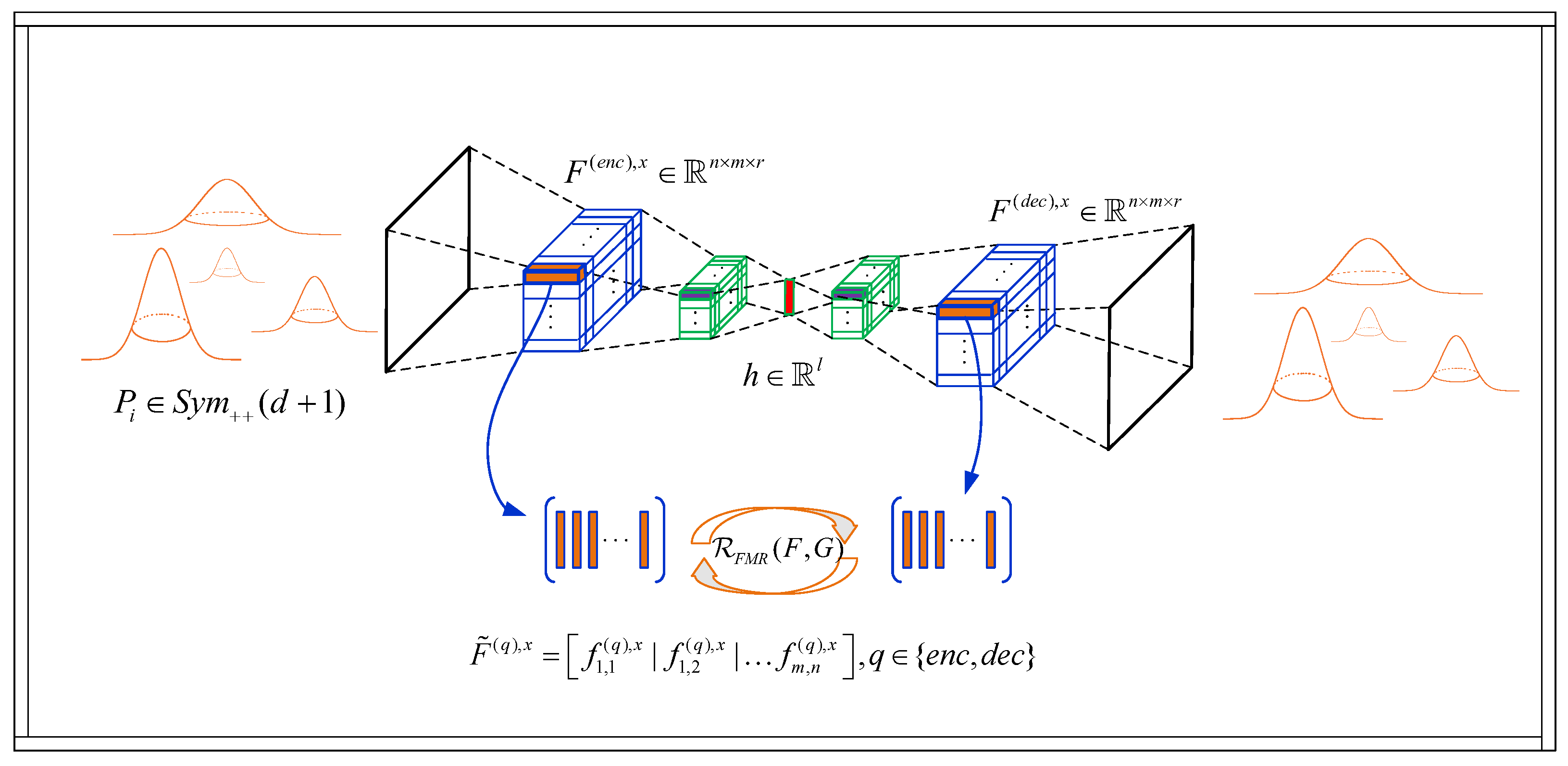
For the second type of deep autoencoder architecture, we use a deep CNN autoencoder, where we observe the model inputs, i.e., the entries of some particular Lovric embedding representative P i (2D SPD matrix), as “pixels” of some 2D image (as usual in vision-based CNNs). This embedding framework consists of the encoder and the decoder CNN networks F and G, respectively, as well as the middle layer h R l , as shown in Figure 2.
The training procedure can be given by the same optimization problem (12) where we use the Frobenious matrix norm · F instead of the Euclidean · l 2 in the objective, as we deal with matrices at the input (as well as at the output) of the CNN autoencoder. Nevertheless, it still requires the strong regularization provided by an additional cost term that forces the similarity between the corresponding feature map tensors in the encoder and the decoder, i.e., the outputs of the convolutional layers corresponding to the encoder and the decoder (between the first feature map of the encoder and the last feature map of the decoder, etc.). Namely, we add the feature map regularization (FMR) penalty term R F M R in the form of a similarity measure between the PDFs that model statistics of the computed feature maps in F and G. Thus, we obtain the CNN autoencoder learning problem as follows:
F ^ , G ^ = argmin F , G E P p ( P ) ( G F ) ( P ) P F + λ R ( F , G ) , + λ F M R R F M R ( F , G )
with some fixed λ F M R > 0 , where · F is the Frobenius norm defined for A = [ a i j ] R m × n as A F = i = 1 m j = 1 n a i j 2 .
For measuring the feature map PDFs, i.e., formulating the R F M R , we consider some of the information-based, as well as the Riemannian manifold-based distances reported in [19,23]. For the low-dimensional Euclidean representation of SPD instances P i Sym + + ( d + 1 ) obtained by the Lovric embedding of Gaussian components, we take the vectors obtained from the middle layer of the deep autoencoder networks, i.e., bottleneck h R l , as described herein. These nonlinear projection quantities are then used to formulate the novel GMM-Autoenc similarity measures that we invoke.

2.2.2. Ground Distances Regularization

We present ground distances between multidimensional (k-dimensional) Gaussians, that we use as similarity measures in order to regularize the training of an autoencoder network, i.e., to form R F M R ( F , G ) . Let us consider k-dimensional f = N ( x ; μ 1 , 1 ) and g = N ( x , μ 2 , 2 ) , which are elements of Sym + + ( k ) , or k + 1 -dimensional SPD Lovric embedding representatives given by (11) as elements of Sym + + ( k + 1 ) , which are both Riemannian manifolds (see [19,23]), equipped with different Riemannian metrics, and inducing geodesic distances. Out of such ground distances that do not take into account the information geometric properties of multidimensional Gaussians, we consider the l 2 -based distance:
d l 2 ( f , g ) = 1 2 F + η μ 1 μ 2 l 2 ,
as well as the robust l 1 -based distance given by:
d l 1 ( f , g ) = 1 2 l 1 + η μ 1 μ 2 l 1 ,
where · l 1 is the robust l 1 norm in R k . We note that the distance functions involving the · l 2 and · F norm in (16) emerge from the assumption that the prior function, i.e., PDF, in the formulation of the regularization problem, is of the Gaussian type. These can be considered as more appropriate ones when there is a large amount of training data, while the ones based on the l 1 norm in (17), which correspond to the prior distribution of Laplace type, are usually used if we tend to obtain a more robust estimation.
Considering that there is a closed-form expression for the KL divergence between two arbitrary Gaussians f and g, denoted by d K L ( f , g ) = K L ( f | | g ) , with K L ( f | | g ) given by (2) (where the symbols are replaced by: d k , f i f , g j g ), for the information-based ground distance, we use the symmetrized version of the KL divergence given by:
d K L s y m ( f , g ) = 1 2 ( d K L ( f , g ) + d K L ( g , f ) ) .
Although the KL divergence is not symmetric, we note that it does not mean that it is antisymmetric. Namely, we give the following counterexample: for two discrete Bernoulli distributions B α ( x ) and B β ( x ) , parameterized by α = p and β = 1 p , respectively, it holds that K L ( B α | | B β ) = K L ( B β | | B α ) .
For the geometrical ground distance, we use Log-Euclidean metric as geodesic distance (see [40]) on Sym + + ( k + 1 ) , forming the efficient geodesic distance invariant to similarity transformation, given by:
d l e , n o n s y m ( P f , P g ) = ln ( P f ) ln ( P g ) F ,
for Lovric embedding SPD representatives P f , P g Sym + + ( k + 1 ) of f and g, respectively. Actually, we use the symmetrized version:
d l e ( P f , P g ) = 1 2 d l e , n o n s y m ( P f , P g ) + d l e , n o n s y m ( P g , P f ) ,

2.2.3. Forming the Feature Map Regularizer R F M R ( F , G )

Let us denote the first feature map tensor of the encoder and the last feature map tensor of the decoder of the CNN autoencoder network, obtained for the input matrix x R ( d + 1 ) × ( d + 1 ) , as F ( e n c ) , x R n × m × r , and F ( d e c ) , x R n × m × r , respectively, (both tensors are of the convolution layers type, and are of identical format, size m × n and depth r, since the encoder and the decoder are assumed to be symmetric). In a general case, for the r-dimensional feature map or layer indexed by q, we will reshape or reformat the F ( q ) , x 3D tensor into the following 2D matrix: F ˜ ( q ) , x = f 1 , 1 ( q ) , x | f 1 , 2 ( q ) , x | f m , n ( q ) , x , q { e n c , d e c } , where f i , j ( q ) , x R r , i { 1 , , n } , j { 1 , , m } are r-dimensional observations (or values) of the autoencoder feature maps in layer q (generated by the corresponding statistics of the autoencoder layer q with depth r).
Next, under the assumption that the underlying PDFs are r-dimensional multivariate Gaussians, i.e., that the unknown PDFs rendering the r-dimensional observations (values in the described feature map tensors) are normally distributed, f i , j ( q ) , x N ( ( q ) , x , μ ( q ) , x ) , we obtain the maximum likelihood estimates (MLEs) of their covariances and centroids, i.e., ^ ( q ) , x , μ ^ ( q ) , x , q { e n c , d e c } from the columns of matrices F ˜ ( q ) , x , q { e n c , d e c } as:
^ ( q ) , x = 1 m n i = 1 m j = 1 n ( f i , j ( q ) , x μ ( q ) , x ) ( f i , j ( q ) , x μ ( q ) , x ) T , μ ^ ( q ) , x = 1 m n i = 1 m j = 1 n f i , j ( q ) , x ,
Finally, we form the feature map regularizer R F M R ( F , G ) in (15) as follows:
R F M R ( F , G ) = E P p ( P ) d g d ( f P , g P )
where f P = N ( ( e n c ) , P , μ ( e n c ) , P ) , g P = N ( ( d e c ) , P , μ ( d e c ) , P ) , and the ground distances g d { l 2 , l 1 , K L s y m , l e } are all defined in the previous section. P Sym + + ( r + 1 ) stands for the SPD matrices generated by p ( P ) , i.e., by the distribution p of Lovric embedding SPD matrices representing the feature map Gaussians described by statistics in (20). Note that each of these Gaussians P, i.e., ( r + 1 ) × ( r + 1 ) SPD matrices made of ^ ( q ) , x and mean μ ^ ( q ) , x in (20), correspond to one of the original Gaussian components brought to the input of the autoencoder, i.e., one input x. In other words, estimates in (20) correspond to the autoencoder feature map observations in R r , while the input Gaussian components are in R d . Since it is assumed that there are M such ( d + 1 ) × ( d + 1 ) SPD matrices corresponding to the individual components of all GMMs present in the training phase of some particular ML task, we estimate the expectation in (21) as:
E P p ( P ) d g d ( f P , g P ) = 1 M i = 1 M d g d ( f P i , g P i ) ,
Thus, M is the overall number of Gaussians of GMMs used for the autoencoder training, and each of the M input Gaussians results in feature map tensors F ( q ) , x , q { e n c , d e c } , i.e., their statistics in (20) are represent by the Lovric embedding P Sym + + ( r + 1 ) in (21).

2.2.4. Forming the GMM Similarity Measure Based on Autoencoder-Generated Representations

We form the proposed novel GMM-Autoenc similarity measures by following the approach similar to that described in [26]. Namely, the similarity measure between two particular GMMs is formed by aggregating the non-negative real values that represent the measure of similarity between corresponding components, i.e., their nonlinear embeddings. Actually, we have to compare the transformed “clouds” of lower l-dimensional Euclidean parameter vectors, with l n , n = ( d + 1 ) ( d + 2 ) / 2 , which are computed from the original Gaussian components of two GMMs. In all approaches that we utilize, for the particular m f -component GMM f = i = 1 m f α i f i with f i = N ( μ i , i ) , we represent GMM by the unique tupple F = ( v 1 , , v m f , α 1 , , α m f ) , which consists of the embedding vectors v i corresponding to the low-dimensional outputs from the middle (bottleneck) layer of the trained embedding autoencoder described in Section 2.2.1. In this process, the belonging mixture weights α i are also taken into account. We note that the autoencoder inputs are the Lovric embeddings of f i , defined by (11), i.e., SPD matrices P i or their vectorized counterparts.
Thus, the similarity measure between two GMMs, denoted by f = i = 1 m f α i f i and g = j = 1 m g β j g j , is introduced as the similarity between the corresponding representatives F = v 1 , , v m f , α 1 , , α m f and G = u 1 , , u m g , β 1 , , β m g , respectively. It is measured in the autoencoder embedding space, as represented by the weighted low-dimensional Euclidean vectors v i , u i R l . By doing so, we utilize two different approaches. The first one employs a form of fuzzy union or intersection operation (see, e.g., [41]). Namely, we use the weighted max–min operator as follows:
p i = min { β j v i u j 2 | j = 1 , , m f } a = max { α i p i | i = 1 , , m g } q j = min { α i v i u j 2 | i = 1 , , m g } b = max { β j q j | j = 1 , , m f } D 1 ( F , G ) = 1 2 ( a + b ) ,
as well as the maximum of the positive weighted sums
a = max { α i j = 1 n β j v i u j 2 | i = 1 , , m g } b = max { β j i = 1 m α i v i u j 2 | j = 1 , , m f } D 2 ( F , G ) = 1 2 ( a + b ) .
In the following, the invoked GMM measures induced by D 1 will be denoted by GMM-Autoenc 1 , A E , for the classical autoencoder architecture and GMM-Autoenc 1 , A E C N N for the CNN autoencoder. Similarly, the GMM measures induced by D 2 will be denoted by GMM-Autoenc 2 , A E and GMM-Autoenc 2 A E C N N , respectively. Both types satisfy self-similarity, positivity, and are symmetric; however, on the contrary to KL divergence, self-identity is not satisfied.
The second aggregation approach utilizes the EMD distance on the F and G representatives of two GMMs that are mutually compared. It is based on the work proposed in [24] and the EMD transportation problem. Namely, the computed tuples F and G are interpreted as the sets of low-dimensional Euclidean vectors equipped with the weights or masses α i , i = 1 m f , and β j , j = 1 m g , respectively. Thus, we introduce the measure of similarity between two GMMs f and g to be the measure between weighted “clouds” F and G consisting of the Euclidean vectors in R l (e.g., see [24]). Taking into account the distance or cost between all pairs of R l vectors from F and G, i.e., by computing the matrix [ d i j ] , it follows that the optimal flow [ ζ i j ] (with the lowest overall cost) when moving R l vectors from F to G is obtained as the solution to the following LP type minimization problem:
min ζ i j i = 1 m f j = 1 m g d i j ζ i j , s . t . ζ i j 0 , i = 1 , , m f , j = 1 , , m g , j = 1 m g ζ i j α i , i = 1 , , m f , i = 1 m f ζ i j β j , j = 1 , , m g , i = 1 m f j = 1 m g ζ i j = 1 .
Based on the optimal flow [ ζ i j ] , it follows that the aggregate EMD distance between the sets of the Euclidean vectors in F and G can be computed as:
D E M D ( F , G ) = i = 1 m f j = 1 m g d i j ζ i j i = 1 m f j = 1 m g ζ i j .
Regarding the LP in (25), [ d i j ] is the matrix of Euclidean distances between vectors v i and u j in R l , i.e., d i j = v i u j 2 . The first constraint imposed on the solution [ ζ i j ] defines the direction of mass or “supplies” flow, i.e., it allows moving supplies from the cloud or set F to the cloud or set G, but not vice versa. We also note that α i as well as β j sums up to be one. The second constraint in (25) limits the amount of supplies that can be sent from F to G, by imposing the restriction that the elements from F individually cannot supply more goods in total to the elements of G than the amount corresponding to the value of their weight in F; while the third constraint puts the same type of restrictions on the elements of G (that they cannot receive more supplies in total than the value of their individual weight, i.e., capacity). The fourth constraint in the form of equality serves the purpose to exploit all available flow from the cloud F to the cloud G (i.e., to move the maximum amount of supplies as possible). Once the transportation problem is solved, the optimal values of [ ζ i j ] are determined, and the Earth mover’s distance D E M D ( F , G ) in (26) is defined as the total work or cost (resulting value of the objective function) that is necessary in order to move, by optimal flow [ ζ i j ] , the maximum amount of supplies possible, from the “cloud” F to the “cloud” G, which is normalized by the total flow (as in the optimal transportation problem).
Moreover, the fact that the EMD distance is a metric (see [24]), implies that the measure of similarity between two GMMs defined by (26) is also a metric. We denote the GMM measures induced by D E M D as GMM-Autoenc 3 , A E and GMM-Autoenc 3 , A E C N N , respectively.

2.3. Computational Complexity

In large-scale ML systems relying on GMMs as a way of modeling distributions of interest, the number of high-dimensional Gaussian components is usually large, which can induce a significant computational burden in cases when the similarity between the GMMs is measured. Therefore, it is of interest to have low-computational complexity, and at the same time, preserve the accuracy of performing the ML task, e.g., recognition, which can be achieved by the baseline KL divergence-based GMM similarity measures. Reducing the computational burden is of the utmost importance in providing efficient services based on such GMM-based ML systems.
Let us assume that the full covariance GMMs f and g have the same number of components m. We denote by d the dimension of the original feature space corresponding to some recognition task. The computational complexity of the Monte Carlo approximation K L M C , defined by relation (1), is estimated as O ( N m d 3 ) , where N is the number of samples. Namely, there are N observations for which two mixtures are calculated, each with m Gaussian components, and the computational complexity for calculating each component is of the order of O ( d 3 ) , so the overall computational complexity is of the order of O ( N m d 3 ) . However, to obtain an efficient KL divergence approximation, the number of i.i.d. samples N must be large, making it inefficient. For the computational complexity of all KL-based measures, K L W A , K L M B , and K L V B , defined in Section 2.1 by relations (3), (4) and (7), respectively, the rationale is as follows. Their complexities are dominated by the term K L ( f i | | g j ) , and there are m 2 such terms, as it is assumed that both mixtures in the pair have m d-variate Gaussian components, so i , j = 1 , , m . As K L ( f i | | g j ) is defined by (2), it can be seen that calculations of these are dominated by the inversion of d-dimensional SPD matrices, which is of the order of O ( d 3 ) . Thus, the overall computation is of the order of O ( m 2 d 3 ) . We use all these in the experiments as the baseline measures.
Concerning the complexity of similarity measures reported in [27], they are estimated as O ( m l ˜ d 2 ) + O ( m d l ˜ 2 ) + O ( m 2 l ˜ 3 ) where l ˜ × l ˜ is the dimension of low-dimensional SPD representatives. We denote the mentioned similarity measures (unsupervised versions) by u D P L M W A , u D P L M M B , and u D P L M V B and use those in the experiments as baseline measures.
The measures reported in [25,26] have complexity estimated by O ( m d 2 l ) + O ( m 2 l ) , where l is the dimensionality of the corresponding low-dimensional embedding. This also holds for GMM measures induced by D 1 and D 2 , as given by (23) and (24), respectively, while D E M D , given by (26), induces the GMM similarity measure with the complexity of the order of O ( m d 2 l ) + O ( m 2 l ) + O ( m 5 ) (as can be seen, e.g., in [25,26]).
Since the proposed GMM-Autoenc i , A E , i = 1 , 2 has a single layer encoder, its computational complexity is influenced by the described aggregation operators, and can be estimated in the same way, i.e., as O ( m d 2 l ) + O ( m 2 l ) , where l is the size of the low-dimensional autoencoder embedding (in the case of the architecture with the input layer, hidden layer, and output layer which is used in the experiments). On the other hand, for GMM-Autoenc i , C N N A E , i = 1 , 2 , if we assume that there are two convolutional feature map layers in the encoder as well as the decoder of the embedding CNN autoencoder, in the case when using D 1 and D 2 given by (23) and (24), the computational complexity of the CNN-based GMM similarity measure can be estimated as O ( 2 m w 1 h 1 k 1 2 n 1 ) + O ( 2 m w 2 h 2 k 2 2 n 1 n 2 ) + O ( 2 m w 3 h 3 k 3 2 n 2 n 3 ) + O ( m 2 l ) . Note that n i , w i , h i , k i < d are the dimensions of the corresponding convolutional layers in the encoder (depth, width, height, and kernel spatial size).
For the proposed EMD-based similarity measure GMM-Autoenc 3 , A E induced by (26), the computational complexity is estimated as O ( m d 2 l ) + O ( m 2 l ) + O ( m 5 ) . Namely, the term O ( m 2 l ) corresponds to the computational complexity of calculating v i u j l 2 between all pairs of l-dimensional representatives of Gaussian components f i and g j , respectively, i , j = 1 , , m . The term O ( m d 2 l ) comes from the encoding process in the autoencoder network. At the input, we have d ( d + 1 ) / 2 ) -dimensional vectors that are transformed by matrix multiplication and nonlinearity into l-dimensional output vectors (from the computational complexity perspective nonlinearity can be neglected if considered to be a piecewise affine). The third term, O ( m 5 ) , comes from the computational complexity of the LP problem given by (25), where the number of iterations in the EMD computation is O ( 2 m ) , as described in [23]. Regarding the GMM-Autoenc 3 , C N N A E , which is based on the CNN autoencoder architecture, the computational complexity can be estimated as O ( 2 m w 1 h 1 k 1 2 n 1 ) + O ( 2 m w 2 h 2 k 2 2 n 1 n 2 ) + O ( 2 m w 3 h 3 k 3 2 n 2 n 3 ) + O ( m 2 l ) + O ( m 5 ) , which has the similar complexity as the previously described Autoenc i , C N N A E , i = 1 , 2 , with only one difference, namely that it has an additional term O ( m 5 ) , originating from solving the LP problem in (25).
It can be seen that the computational complexity of the proposed GMM-Autoenc i , A E for i = 1 , 2 , 3 , i.e., when using D 1 and D 2 and D E M D , is similar to the corresponding GMM similarity measures reported in [25,26], which is thus computationally significantly more efficient when compared with K L W A , K L M B , and K L V B . Depending on the relation between l ˜ and l, the proposed autoencoder-based measures are also potentially more efficient when compared with unsupervised u D P L M W A , u D P L M M B , u D P L M V B , and the supervised s D P L M W A , s D P L M M B , and s D P L M V B . The computational complexity of the proposed GMM-Autoenc i , C N N A E , i = 1 , 2 , 3 is also significantly more efficient when compared with K L W A , K L M B , and K L V B , but less efficient than GMM-Autoenc i , A E , i = 1 , 2 , 3 .

3. Experimental Results

In this section, the network architecture used in the experiments, as well as the experimental results of applications of the proposed novel GMM-Autoenc similarity measures are presented. The comparisons include several baseline measures given in Section 2.1, over various datasets within a texture recognition task.

3.1. Network Architectures

In the case of the fully connected autoencoder utilized in GMM-Autoenc i , A E , i = { 1 , 2 } , we used a simple fully connected architecture consisting of input and output layers with one hidden representation layer between them and the logistic sigmoid transfer function. The training consisting of scaled conjugate gradient descent optimization was driven by the MSE loss function defined in (13), accompanied by the l 2 weight regularization term R ( F , G ) defined in (14), and the regularization penalty λ = 10 . The number of nodes in the input and output layers was determined by the dimensionality of the input and output feature space. The CNN encoder utilized in GMM-Autoenc i , C N N A E , i = { 1 , 2 } consists of three convolutional layers narrowing down the higher-dimensional input (matrices of size d × d ) into lower-dimensional vectors R l , while preserving the relevant clustering information. The depths of CNN layers are n 1 = 32 , n 2 = 64 , and n 3 = 128 , with the square kernel sizes of k 1 = 14 , k 2 = 7 , and k 3 = 3 . The dimensions of the layers’ width w i and height h r , r = { 1 , 2 , 3 } are implicitly determined by the size of input SPD matrices, but we note that the stride value was 2. The bottleneck layer of size R l is connected to the last CNN layer by one flattening layer and two additional linear layers with a ReLU component in between. ReLU components are also added among convolutional layers, including one batch norm regularizer between the last two convolutional layers. The CNN decoder architecture replicates the above-described pattern in the backward order, decompressing the latent feature space into the original matrix features. For CNN autoencoder training, the Adam gradient descent optimization algorithm is applied. Adaptive optimization algorithms, such as Adam, have shown a better optimization performance in the means of faster convergence, due to the adaptive learning rate, as can be seen in [42]. Moreover, empirical results demonstrate that Adam works well in practice and still achieves a competitive performance when compared with newer methods, as can be seen in [43]. The procedure is performed by using the objective defined in (15) over 30 epochs, with a learning rate of 0.001 , a learning decay rate decay of 1 e 05 , and the feature map regularization term R FMR ( F , G ) defined in (21), with a regularization penalty value of λ F M R = 10 . The first regularization term R ( F , G ) in (15) refers to network weights and is of the same type as in the case of previously described GMM-Autoenc i , A E . In both cases, all input matrices (from both the training and test data instances) have been normalized to the [0,1] range before the actual training.

3.2. Performances

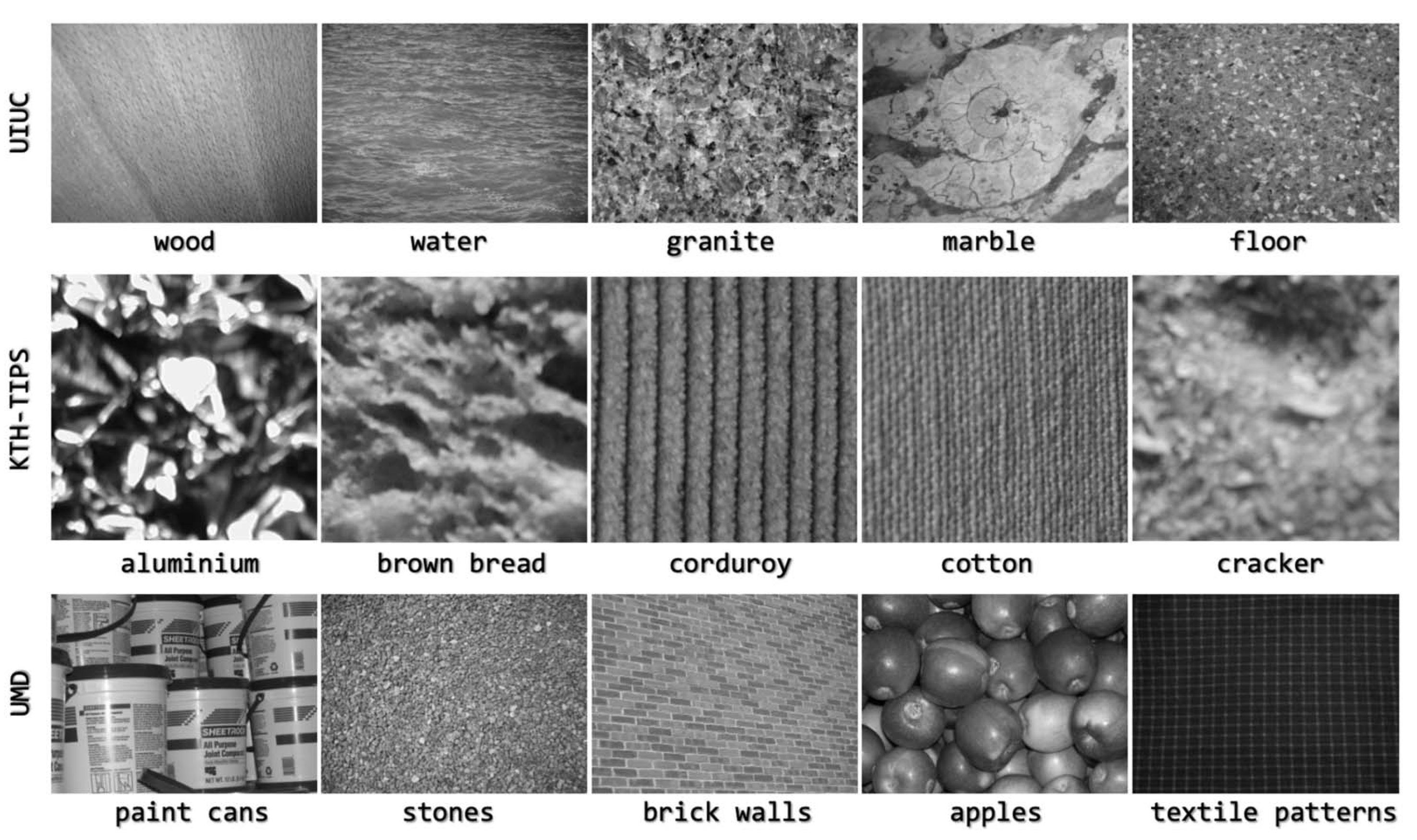
Experimental results are given for the proposed GMM-Autoenc-based similarity measures invoked in Section 2.2 and Section 2.2.4, compared to baseline KL-based measures K L W A , K L M B and K L V B given by (3), (4), and (7), respectively, and proposed in [1,2]; as well as to the baseline EMD-based unsupervised u D P L M W A , u D P L M M B , u D P L M V B measures, proposed in [27]. Experiments were conducted within the texture recognition tasks on the UIUC texture dataset, the KTH-TIPS image dataset, and the UMD texture dataset. A five-class recognition problem is considered in all experiments. Concerning the UIUC dataset, the following classes are considered: wood, water, granite, marble, and floor, with images of 640 × 480 pixel resolution. In the case of the KTH-TIPS dataset, the following classes were considered: aluminum foil, brown bread, corduroy, cotton, and cracker, with images of 1280 × 960 pixel resolution. Finally, for the UMD texture dataset, we used images from the following classes: paint cans, stones, brick walls, apples, and textile patterns, sampled at 1280 × 960 pixels. Selected samples from all three databases are shown in Figure 3.
Concerning the underlying texture features used for the experiments as texture descriptors, the region covariance descriptors proposed in [30] are employed, since they have already shown good performance in various texture recognition tasks (see for example [19,23,27,30]). For any given N × M image, they are formed in the following way: patches of size m × m , m < min { N , M } are cropped ( m = 128 with the step size of 16 for the UIUC dataset, m = 40 with the step size of 5 for the KTH-TIPS dataset and m = 256 with the step size of 32 for the UMD dataset). For every pixel positioned at ( x , y ) , features were calculated as elements of R d ^ , d ^ = 5 , i.e., [ I , | I x | , | I y | , | I x x | , | I y y | ] , where I represents illumination, I x and I y are the first-order derivatives and I x x and I y y are the second-order derivatives. Covariance matrices were calculated for the mentioned features and their upper triangular part is vectorized into d = d ^ ( d ^ + 1 ) / 2 = 15 -dimensional feature vectors. The parameters of GMMs are then estimated using the EM algorithm (as can be seen in [44]) applied over the pool of feature vectors obtained as previously described. During experiments, for every n × m -size image in all mentioned datasets, the uniform sampling of the N s m p l sub-images of the size of ( n / 2 ) × ( m / 2 ) is performed in order to augment every database, which is needed to train a nonlinear autoencoder in order to perform the GMM-Autoenc measure (deep autoencoder in the case of GMM-Autoenc 1 , A E C N N ), because originally, we do not have a sufficient amount of data in order to train them. Every GMM (or its low-dimensional Euclidean or SPD representatives for the proposed GMM-Autoenc or DPLM GMM similarity measures, respectively) is compared to all other GMMs in the training set, and its class is determined using the KNN method.
In Table 1, Table 2 and Table 3, the performances of the novel GMM-Autoenc GMM similarity measures are presented when compared with KL-based as well as DPLM-based measures, for the UIUC, KTH-TIPS, and UMD datasets, respectively. In all experiments, the number of Gaussian components used to represent any particular training or testing image was set to m { 1 , 5 , 10 } . For the case of DPLM-based and GMM-Autoenc measures, K = 3 for the KNN, and the projection dimension for DPLM-based methods was set to l ˜ { 5 , 7 } . Results in Table 1, Table 2 and Table 3 for the proposed GMM-Autoenc i , A E C N N refer to the model training procedure with FMR regularization based on the log-Euclidean ground distance g d = l e given in (19), as we obtained slightly better results with this regularizer when compared with other ground distances.
From the experimental results presented in Table 1, Table 2 and Table 3, which correspond to recognition accuracy, and taking into account the computational complexity analyses given in Section 2.3, it can be seen that all of the proposed novel GMM-Autoenc measures obtained a better trade-off between recognition accuracy and computational complexity for all datasets when compared with the baseline KL-based as well as DPLM-based measures mentioned in Section 2.2. We note that GMM-Autoenc i , A E variants could be the preferred choice when compared with GMM-Autoenc i , A E C N N models, probably due to the number of training samples in all datasets, which is relatively small for the training of a CNN architecture.

4. Conclusions

In this work, a novel similarity measure between GMMs based on autoencoder-generated Gaussian component representations is proposed. Low-dimensional Euclidean vectors obtained using nonlinear autoencoder embedding demonstrated higher similarity measurement capabilities when compared with the existing baseline models. Two different approaches were explored and utilized to encode the original Gaussian mixture components. The first one focused on the simple architecture of the classical autoencoder, where the vectorized versions of the SPD matrices obtained by the Lovric embedding of GMM Gaussians were used to generate inputs for the fully connected autoencoder. In the second approach, a more complex CNN autoencoder was utilized in combination with the novel regularization training in the feature space. In terms of trade-off between the recognition accuracy and the computational complexity, autoencoder embedding proved to be a better solution when compared with the existing GMM similarity measurement baselines in texture recognition tasks. In general, any domain in which some random processes, data instances, or groups of entities are described by PDFs in the form of Gaussian mixture models can be considered as possible fields of application that would benefit from the proposed computationally efficient GMM similarity measures. Besides ML recognition tasks based on decision rules in the form of minimum distance classifiers, we also foresee various applications in other domains such as clustering, probabilistic modeling, kriging methods, learning regularization, and feature space alignment as possible extensions of the current study and proposed similarity measures. For more effective dimensionality reduction, the utilized autoencoder networks should be trained on large datasets, but this could be performed in various settings, online or offline, or by designing encoders for specific sub-tasks and data modalities. In that sense, described methods are scalable and could be adapted to specific system requirements. Thus, in order to fully explore the capabilities of the CNN-based embedding approach, in future work, we plan to conduct experiments on tasks with much larger datasets and different data modalities.

Author Contributions

Conceptualization, V.K. and M.J.; methodology, V.K. and B.P.; software, B.P.; validation, B.B.; formal analysis, M.J. and N.R.; investigation, V.K., M.J. and B.P.; resources, B.P.; data curation, M.J.; writing—original draft preparation, M.J. and B.P.; writing—review and editing, B.B.; visualization, B.P. and B.B.; supervision, N.R.; project administration, B.P.; funding acquisition, B.B. All authors have read and agreed to the published version of the manuscript.

Funding

This research was supported by the Serbian Ministry of Education, Science and Technological Development through project no. 45103-68/2020-14/200156: “Innovative Scientific and Artistic Research from the Faculty of Technical Sciences Activity Domain”, and the internal project of the Faculty of Technical Sciences in 2023: “Research aimed at improving the teaching process and development of scientific and professional areas of the Department of Power, Electronic and Telecommunication engineering”. This research also received publication fee support from the H2020 project INCOMING (ID 856967): “Innovation and excellence in massive-scale communications and information processing”.

Data Availability Statement

Publicly available datasets were analyzed in this study. The UIUC data description can be found in [45], and data can be found here: http://www.cvr.ai.uiuc.edu/ponce_grp, accessed on 1 September 2016. KTH-TIPS data description can be found in [46], and data can be found here: https://www.csc.kth.se/cvap/databases/kth-tips, accessed on 1 October 2022. UMD data description can be found in [47], and data can be found here: http://users.umiacs.umd.edu/~fer/website-texture/texture.htm, accessed on 3 December 2022.

Acknowledgments

The authors would also like to acknowledge the ICONIC centre—Centre for Intelligent Communications, Networking and Information Processing (https://iconic.ftn.uns.ac.rs/); established through H2020 project INCOMING (ID 856967) at the Faculty of Technical Sciences in Novi Sad.

Conflicts of Interest

The authors declare no conflict of interest. The funders had no role in the design of the study; in the collection, analyses or interpretation of data; in the writing of the manuscript; or in the decision to publish the results.

Abbreviations

The following abbreviations are used in this manuscript:
AIArtificial Intelligence
CNNConvolutional Neural Network
DNNDeep Neural Network
DPLMDistance Preservation to the Local Mean
EMExpectation Maximization
EMDEarth Mover’s Distance
FMRFeature Map Regularized
GMMGaussian Mixture Model
KLKullback–Leibler
KNNK-Nearest Neighbors
KTHRoyal Institute of Technology in Stockholm
LPLinear Programming
MBMatching-Based
MCMonte Carlo
MLMachine Learning
MLEMaximum Likelihood Estimate
MSEMean Squared Error
PDFProbability Density Function
SPDSymmetric Positive Definite
TIPSTextures Under Varying Illumination, Pose and Scale
UCUnscented Transform
UIUCUniversity of Illinois Urbana-Champaign
UMDUniversity of Maryland
VBVariational Bound
VAEVariational AutoEncoder
WAWeighted Average

References

  1. Goldberger, J.; Aronowitz, H. A distance measure between GMMs based on the unscented transform and its application to speaker recognition. In Proceedings of the INTERSPEECH, Lisbon, Portugal, 4–8 September 2005; pp. 1985–1988. [Google Scholar]
  2. Goldberger, J.; Gordon, S.; Greenspan, H. An efficient image similarity measure based on approximations of KL-divergence between two Gaussian mixtures. In Proceedings of the International Conference on Computer Vision, Nice, France, 13–16 October 2003; Volume 3, pp. 487–493. [Google Scholar]
  3. Wu, Y.; Chan, K.L.; Huang, Y. Image texture classification based on finite Gaussian mixture models. In Proceedings of the 3rd Int. Workshop on Text. Anal. and Synth., Int. Conf. on Computer Vision, Nice, France, 13–16 October 2003; pp. 107–112. [Google Scholar]
  4. Dilokthanakul, N.; Mediano, P.A.; Garnelo, M.; Lee, M.C.; Salimbeni, H.; Arulkumaran, K.; Shanahan, M. Deep unsupervised clustering with Gaussian mixture variational autoencoders. arXiv 2017, arXiv:1611.02648v2. [Google Scholar]
  5. Gangodkar, D. A novel image retrieval technique based on semi supervised clustering. Multimed. Tools Appl. 2021, 80, 35741–35769. [Google Scholar] [CrossRef]
  6. Asheri, H.; Hosseini, R.; Araabi, B.N. A new EM algorithm for flexibly tied GMMs with large number of components. Pattern Recognit. 2021, 114, 107836. [Google Scholar] [CrossRef]
  7. Durrieu, J.L.; Thiran, J.P.; Kelly, F. Lower and upper bounds for approximation of the Kullback-Leibler divergence between Gaussian mixture models. In Proceedings of the International Conference on Acoustics, Speech and Signal Processing, Kyoto, Japan, 25–30 March 2012; pp. 4833–4836. [Google Scholar]
  8. Brkljač, B.; Janev, M.; Obradović, R.; Rapaić, D.; Ralević, N.; Crnojević, V. Sparse representation of precision matrices used in GMMs. Appl. Intell. 2014, 41, 956–973. [Google Scholar] [CrossRef]
  9. Kaur, A.; Sachdeva, R.; Singh, A. Classification approaches for automatic speech recognition system. In Artificial Intelligence and Speech Technology; CRC Press: Boca Raton, FL, USA, 2021; pp. 1–7. [Google Scholar]
  10. Demir, K.E.; Eskil, M.T. Improved microphone array design with statistical speaker verification. Appl. Acoust. 2021, 175, 107813. [Google Scholar] [CrossRef]
  11. Yücesoy, E. Two-level classification in determining the age and gender group of a speaker. Int. Arab J. Inf. Technol. 2021, 18, 663–670. [Google Scholar] [CrossRef]
  12. Narasimhan, H.; Vinayakumar, R.; Mohammad, N. Unsupervised deep learning approach for in-vehicle intrusion detection system. IEEE Consum. Electron. Mag. 2023, 12, 103–108. [Google Scholar] [CrossRef]
  13. Chernoff, H. A measure of asymptotic efficiency for tests of a hypothesis based on the sum of observations. Ann. Math. Stat. 1952, 23, 493–507. [Google Scholar] [CrossRef]
  14. Bhattacharyya, A. On a measure of divergence between two statistical populations defined by their probability distribution. Bull. Calcutta Math. Soc. 1943, 35, 99–110. [Google Scholar]
  15. Matusita, K. Decision rules, based on the distance, for problems of fit, two samples, and estimation. Ann. Math. Stat. 1955, 26, 631–640. [Google Scholar] [CrossRef]
  16. Kullback, S.; Leibler, R.A. On Information and Sufficiency. Ann. Math. Stat. 1951, 22, 79–86. [Google Scholar] [CrossRef]
  17. Kullback, S. Information Theory and Statistics; Dover Publications Inc.: Mineola, NY, USA, 1968. [Google Scholar]
  18. Minh, H.Q.; Murino, V. Covariances in computer vision and machine learning. Synth. Lect. Comput. Vis. 2017, 7, 1–170. [Google Scholar] [CrossRef]
  19. Hao, H.; Wang, Q.; Li, P.; Zhang, L. Evaluation of ground distances and features in EMD-based GMM matching for texture classification. Pattern Recognit. 2016, 57, 152–163. [Google Scholar] [CrossRef]
  20. Nielsen, F. Chernoff information of exponential families. arXiv 2011, arXiv:1102.2684. [Google Scholar]
  21. Mak, H.W.L.; Han, R.; Yin, H.H. Application of variational autoEncoder (VAE) model and image processing approaches in game design. Sensors 2023, 23, 3457. [Google Scholar] [CrossRef]
  22. Lucas, S.M.; Volz, V. Tile pattern KL-divergence for analysing and evolving game levels. In Proceedings of the Genetic and Evolutionary Computation Conference, Prague, Czech Republic, 13–17 July 2019; pp. 170–178. [Google Scholar]
  23. Li, P.; Wang, Q.; Zhang, L. A novel earth mover’s distance methodology for image matching with Gaussian mixture models. In Proceedings of the IEEE International Conference on Computer Vision, Sydney, Australia, 1–8 December 2013; pp. 1689–1696. [Google Scholar]
  24. Rubner, Y.; Tomasi, C.; Guibas, L.J. The earth mover’s distance as a metric for image retrieval. Int. J. Comput. Vis. 2000, 40, 99. [Google Scholar] [CrossRef]
  25. Krstanović, L.; Ralević, N.M.; Zlokolica, V.; Obradović, R.; Mišković, D.; Janev, M.; Popović, B. GMMs similarity measure based on LPP-like projection of the parameter space. Expert Syst. Appl. 2016, 66, 136–148. [Google Scholar] [CrossRef]
  26. Popović, B.; Cepova, L.; Cep, R.; Janev, M.; Krstanović, L. Measure of similarity between GMMs by embedding of the parameter space that preserves KL divergence. Mathematics 2021, 9, 957. [Google Scholar] [CrossRef]
  27. Popović, B.; Janev, M.; Krstanović, L.; Simić, N.; Delić, V. Measure of similarity between GMMs based on geometry-aware dimensionality reduction. Mathematics 2022, 11, 175. [Google Scholar] [CrossRef]
  28. He, X.; Niyogi, P. Locality preserving projections. In Proceedings of the Advances in Neural Information Processing Systems, Vancouver, BC, Canada, 9–14 December 2003; Volume 16. [Google Scholar]
  29. He, X.; Cai, D.; Yan, S.; Zhang, H.J. Neighborhood preserving embedding. In Proceedings of the International Conference on Computer Vision, Beijing, China, 17–21 October 2005; Volume 2, pp. 1208–1213. [Google Scholar]
  30. Sivalingam, R.; Boley, D.; Morellas, V.; Papanikolopoulos, N. Tensor sparse coding for region covariances. In Proceedings of the European Conference on Computer Vision, Heraklion, Greece, 5–11 September 2010; pp. 722–735. [Google Scholar]
  31. Lovrić, M.; Min-Oo, M.; Ruh, E.A. Multivariate normal distributions parametrized as a Riemannian symmetric space. J. Multivar. Anal. 2000, 74, 36–48. [Google Scholar] [CrossRef]
  32. Roy, S.S.; Hossain, S.I.; Akhand, M.; Murase, K. A robust system for noisy image classification combining denoising autoencoder and convolutional neural network. Int. J. Adv. Comput. Sci. Appl. 2018, 9, 224–235. [Google Scholar] [CrossRef]
  33. Ahmed, A.S.; El-Behaidy, W.H.; Youssif, A.A. Medical image denoising system based on stacked convolutional autoencoder for enhancing 2-dimensional gel electrophoresis noise reduction. Biomed. Signal Process. Control 2021, 69, 102842. [Google Scholar] [CrossRef]
  34. Munir, N.; Park, J.; Kim, H.J.; Song, S.J.; Kang, S.S. Performance enhancement of convolutional neural network for ultrasonic flaw classification by adopting autoencoder. NDT E Int. 2020, 111, 102218. [Google Scholar] [CrossRef]
  35. Hershey, J.R.; Olsen, P.A. Approximating the Kullback Leibler divergence between Gaussian mixture models. In Proceedings of the International Conference on Acoustics, Speech and Signal Processing, Honolulu, HI, USA, 15–20 April 2007; Volume 4, pp. 317–320. [Google Scholar]
  36. Cover, T.M. Elements of Information Theory; Wiley Series in Telecommunications; John Wiley & Sons: New York, NY, USA, 1991. [Google Scholar]
  37. Julier, S.J. A General Method for Approximating Non-Linear Transformations of Probability Distributions; Technical Report; Robotics Research Group, Department of Engineering Science, University of Oxford: Oxford, UK, 1996. [Google Scholar]
  38. Ling, H.; Okada, K. An efficient earth mover’s distance algorithm for robust histogram comparison. IEEE Trans. Pattern Anal. Mach. Intell. 2007, 29, 840–853. [Google Scholar] [CrossRef]
  39. Davoudi, A.; Ghidary, S.S.; Sadatnejad, K. Dimensionality reduction based on distance preservation to local mean for symmetric positive definite matrices and its application in brain–computer interfaces. J. Neural Eng. 2017, 14, 036019. [Google Scholar] [CrossRef]
  40. Arsigny, V.; Fillard, P.; Pennec, X.; Ayache, N. Fast and simple calculus on tensors in the log-Euclidean framework. In Proceedings of the International Conference on Medical Image Computing and Computer-Assisted Intervention, Palm Springs, CA, USA, 26–29 October 2005; pp. 115–122. [Google Scholar]
  41. Klir, G.J.; Yuan, B. Fuzzy Sets and Fuzzy Logic: Theory and Applicaions; Prentice Hall New Jersey: Hoboken, NJ, USA, 1995; Volume 4. [Google Scholar]
  42. Kingma, D.P.; Ba, J. Adam: A Method for Stochastic Optimization. In Proceedings of the 3rd International Conference on Learning Representations, San Diego, CA, USA, 7–9 May 2015. [Google Scholar]
  43. Schmidt, R.M.; Schneider, F.; Hennig, P. Descending through a crowded valley-benchmarking deep learning optimizers. In Proceedings of the International Conference on Machine Learning, PMLR, Virtual, 18–24 July 2021; pp. 9367–9376. [Google Scholar]
  44. Webb, A.R. Statistical Pattern Recognition; John Wiley & Sons: Hoboken, NJ, USA, 2003. [Google Scholar]
  45. Lazebnik, S.; Schmid, C.; Ponce, J. A sparse texture representation using local affine regions. IEEE Trans. Pattern Anal. Mach. Intell. 2005, 27, 1265–1278. [Google Scholar] [CrossRef] [PubMed]
  46. Fritz, M.; Hayman, E.; Caputo, B.; Eklundh, J.O. The Kth-Tips Database; Technical Report; Computational Vision and Active Perception Laboratory, Department of Numerical Analysis and Computer Science: Stockholm, Sweden, 2004; Available online: https://www.csc.kth.se/cvap/databases/kth-tips/doc/ (accessed on 1 October 2022).
  47. Xu, Y.; Ji, H.; Fermüller, C. Viewpoint invariant texture description using fractal analysis. Int. J. Comput. Vis. 2009, 83, 85–100. [Google Scholar] [CrossRef]
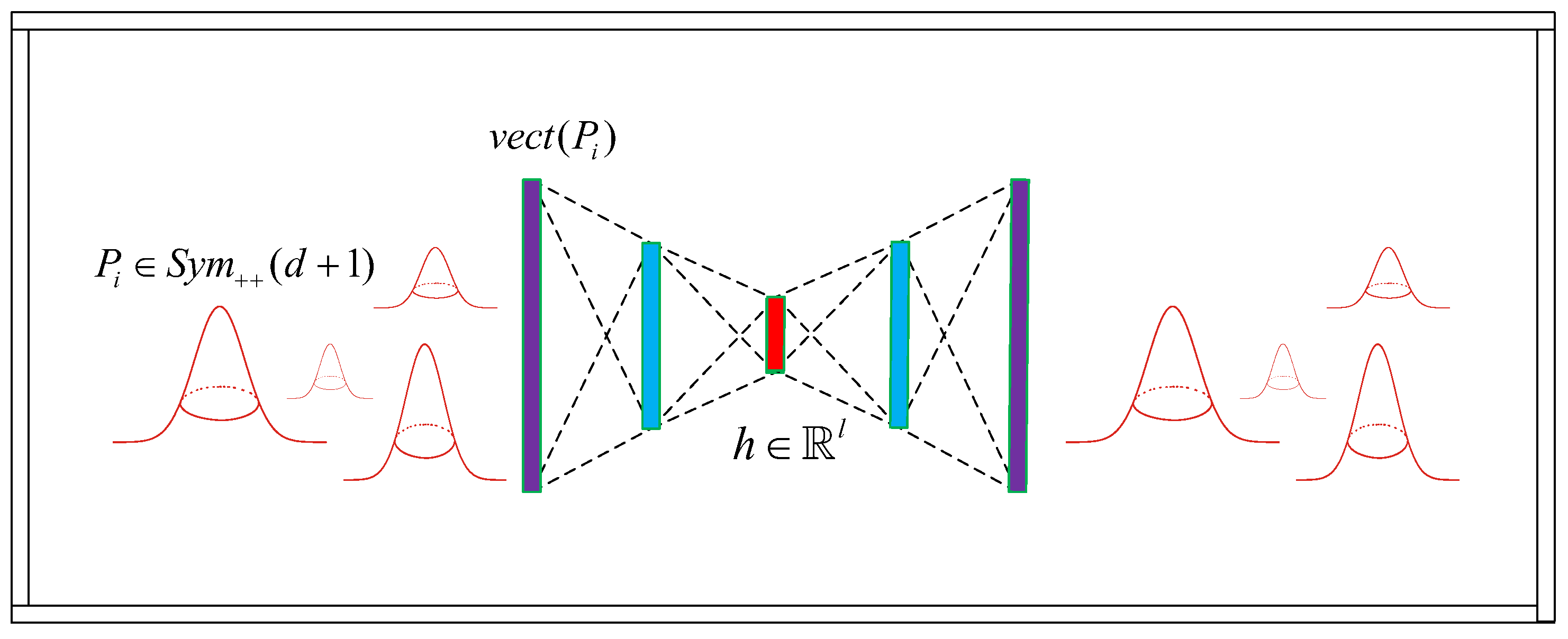
Figure 1. Illustration of the proposed fully connected autoencoder architecture for the low-dimensional embedding of Gaussian components represented by v e c t ( P i ) into h R l . Colors indicate symmetric architecture of the network and the goal of learning unique embedding of the original Gaussian components (middle vector h shown in red).
Axioms 12 00535 g001
Figure 2. Illustration of the proposed FMR regularized CNN autoencoder for the low-dimensional embedding of Gaussian components represented by SPD matrices P i Sym + + ( d + 1 ) into h R l .
Axioms 12 00535 g002
Figure 3. UIUC, KTH-TIPS, and UMD database samples.
Axioms 12 00535 g003
Table 1. Recognition accuracies for the proposed GMM-Autoenc-based measures when compared with KL-based as well as DPLM-based GMM similarity measures on UIUC database.
GMM Sim. Meas. Accuracy
m  = 1 m  = 5 m  = 10
K L M B 0.820.800.80
K L W A 0.820.820.82
K L V B 0.820.820.82
l ˜  = 5 l ˜  = 7 l ˜  = 5 l ˜  = 7 l ˜  = 5 l ˜  = 7
u D P L M M B 0.720.810.730.740.790.79
u D P L M W A 0.720.810.730.740.800.80
u D P L M V B 0.720.810.730.740.800.80
l  = 20 l  = 30 l  = 20 l  = 30 l  = 20 l  = 30
GMM-Autoenc 1 , A E 0.750.810.750.760.800.80
GMM-Autoenc 2 , A E 0.750.810.760.760.800.80
GMM-Autoenc 3 , A E 0.760.800.760.770.810.81
GMM-Autoenc 1 , A E C N N 0.750.800.730.770.810.80
GMM-Autoenc 2 , A E C N N 0.760.810.710.780.810.81
GMM-Autoenc 3 , A E C N N 0.770.810.710.790.810.80
Table 2. Recognition accuracies for the proposed GMM-Autoenc-based measures when compared with KL-based as well as DPLM-based GMM similarity measures on KTH-TIPS database.
GMM Sim. Meas. Accuracy
m  = 1 m  = 5 m  = 10
K L M B 0.780.740.75
K L W A 0.780.780.78
K L V B 0.780.780.78
l ˜  = 5 l ˜  = 7 l ˜  = 5 l ˜  = 7 l ˜  = 5 l ˜  = 7
u D P L M M B 0.570.730.690.710.630.72
u D P L M W A 0.570.730.720.750.640.75
u D P L M V B 0.570.730.720.750.630.75
l  = 20 l  = 30 l  = 20 l  = 30 l  = 20 l  = 30
GMM-Autoenc 1 , A E 0.710.750.730.750.720.74
GMM-Autoenc 2 , A E 0.710.740.720.740.720.75
GMM-Autoenc 3 , A E 0.720.750.730.750.730.76
GMM-Autoenc 1 , A E C N N 0.720.750.730.740.730.73
GMM-Autoenc 2 , A E C N N 0.730.750.710.750.740.76
GMM-Autoenc 3 , A E C N N 0.730.760.720.770.740.77
Table 3. Recognition accuracies for the proposed GMM-Autoenc-based measures when compared with KL-based as well as DPLM-based GMM similarity measures on UMD database.
GMM Sim. Meas. Accuracy
m = 1m = 5m = 10
K L M B 0.750.730.72
K L W A 0.750.750.75
K L V B 0.750.750.75
l ˜  = 5 l ˜  = 7 l ˜  = 5 l ˜  = 7 l ˜  = 5 l ˜  = 7
u D P L M M B 0.730.740.720.720.700.72
u D P L M W A 0.730.740.730.740.710.75
u D L P M V B 0.730.740.730.740.710.75
l  = 20 l  = 30 l  = 20 l  = 30 l  = 20 l  = 30
GMM-Autoenc 1 , A E 0.740.740.730.730.710.72
GMM-Autoenc 2 , A E 0.730.740.730.740.730.74
GMM-Autoenc 3 , A E 0.740.750.740.750.730.75
GMM-Autoenc 1 , A E C N N 0.740.750.730.730.720.72
GMM-Autoenc 2 , A E C N N 0.750.750.740.750.740.74
GMM-Autoenc 3 , A E C N N 0.740.750.740.750.740.75
Disclaimer/Publisher’s Note: The statements, opinions and data contained in all publications are solely those of the individual author(s) and contributor(s) and not of MDPI and/or the editor(s). MDPI and/or the editor(s) disclaim responsibility for any injury to people or property resulting from any ideas, methods, instructions or products referred to in the content.