Article

Slow Manifolds for Stochastic Koper Models with Stable Lévy Noises

by
Hina Zulfiqar
1,
Shenglan Yuan
2,3,* and
Muhammad Shoaib Saleem
1
1
Department of Mathematics, University of Okara, Okara 56300, Pakistan
2
Institut für Mathematik, Universität Augsburg, 86135 Augsburg, Germany
3
Center for Mathematical Sciences, Huazhong University of Science and Technology, Wuhan 430074, China
*
Author to whom correspondence should be addressed.
Axioms 2023, 12(3), 261; https://doi.org/10.3390/axioms12030261
Submission received: 8 December 2022 / Revised: 16 February 2023 / Accepted: 21 February 2023 / Published: 3 March 2023
(This article belongs to the Special Issue Statistical Methods and Applications)

Abstract

:
The Koper model is a vector field in which the differential equations describe the electrochemical oscillations appearing in diffusion processes. This work focuses on the understanding of the slow dynamics of a stochastic Koper model perturbed by stable Lévy noise. We establish the slow manifold for a stochastic Koper model with stable Lévy noise and verify exponential tracking properties. We also present two practical examples to demonstrate the analytical results with numerical simulations.

1. Introduction

The Koper model [1] is an idealized model of the chemical reaction described in [2]. Invariant manifolds are useful in investigating the dynamical behavior of the multiscale systems [3,4]. Invariant manifolds for investigating the dynamical behavior of deterministic systems without being influenced by stochastic forces are discussed in [5,6,7], while invariant manifolds for deterministic systems influenced by stochastic forces are constructed in [8,9,10]. An invariant manifold for a fast-slow stochastic system in which fast mode is indicated by the slow mode tends to slow the manifold when the scale parameter goes to zero. Moreover, the slow manifold converges to a critical manifold as the scale parameter approaches zero.
A slow manifold for a stochastic system driven by Brownian motion is demonstrated in [11,12,13], and its numerical simulations are presented in [14,15]. Lévy motions arise from the models for fluctuations, and they have independent, stationary increments and discontinuous paths. For example, Lévy processes affect the evolution of the state variables in the turbulent flow of fluids [16]. Some models about stochastic systems processed by Lévy noise are explained in [17,18,19]. The slow manifolds under Lévy noise are constructed in [20]. The existence of a slow manifold for nonlocal fast-slow stochastic evolutionary equations is proved in [21,22]. An invariant manifold of variable stability in the Koper model is established in [2]. It continues to be an active topic on the characterization of a stochastic Koper model driven by the Lévy process for both theoretical reasons and applications.
The goal of this article is to construct a three-dimensional stochastic Koper model in Euclidean space R 3 and establish the existence of a slow manifold for a stochastic Koper model processed by α -stable Lévy noise with α ( 1 , 2 ) . Namely, we consider the stochastic Koper system in the following version:
x ˙ = 1 ϵ [ k y x 3 + 3 x λ ( z ) ] + σ ϵ 1 α L ˙ t α , y ˙ = x 2 y + z , z ˙ = ϵ ^ ( y z ) ,
where k and λ ( z ) are the main bifurcation parameters. Here, ϵ ^ = 1 , but ϵ represents a small parameter with the property 0 < ϵ 1 , and it indicates the ratio of two times scales such that stochastic fast-slow system (1) has one fast variable x, and two slow variables y and z. The dot stands for the differentiation with respect to time t. The noise L t α is a two-sided symmetric α -stable Lévy process taking real values, with the stability index α ( 1 , 2 ) and the intensity σ > 0 ; see the references [6,23].
We start from a random transformation such that a solution of a stochastic Koper model (1) can be expressed as a transformed solution of some random system. The establishment of a slow manifold for a defined random system is proved by the utilization of the Lyapunov–Perron method [9,24].
The article is organized as follows: In Section 2, some concepts about random dynamical systems, and stochastic differential equations processed by Lévy motion are discussed. In Section 3, the stability of the stochastic Koper system (1) is proved and a random transformation is defined, which converts stochastic Koper system (1) into a random system. In Section 4, a short review about random invariant manifolds and the existence of an exponential tracking slow manifold for random systems is provided. In Section 5, we present numerical results using two examples from electrochemical oscillations to corroborate our analytical results. Finally, Section 6 summarizes our findings as well as directions for future study.

2. Preliminaries

In this section, some concepts about the random dynamical system are given.
Definition 1.
Let ( Ω , F , P ) be a probability space and θ = { θ t } t R be a flow on Ω satisfying the conditions
  • θ 0 = Id Ω ;
  • θ t 1 θ t 2 = θ t 1 + t 2 , where t 1 , t 2 R ;
and the mapping θ : R × Ω Ω can be defined by ( t , ω ) θ t ω , which is B ( R ) F F measurable. Here, we consider that the probability measure P is invariant with respect to the flow { θ t } t R , i.e., θ t P = P for all t R . Then, Θ = ( Ω , F , P , θ ) is said to be a metric dynamical system [20].
Throughtout this article, we use a scalar Lévy process. Take L t α , α ( 1 , 2 ) as a symmetric two-sided α -stable Lévy process with values in R . Consider a canonical sample space for it. Let Ω = D ( R , R ) be the space of càdlàg functions having zero value at t = 0 , i.e.,
D ( R , R ) = ω : for t R , lim s t ω ( s ) = ω ( t ) , lim s t ω ( s ) = ω ( t ) exist and ω ( 0 ) = 0 .
If we use a standard usual open-compact metric, then the space D ( R , R ) may not be separable and complete. However, the space D ( R , R ) of real-valued càdlàg functions can be extended by introducing another metric d 0 since it can be made into the complete and separable space on a unit interval or on R [25]. For functions ω 1 , ω 2 D ( R , R ) , d 0 ( ω 1 , ω 2 ) is defined by
d 0 ( ω 1 , ω 2 ) = inf ε > 0 : | ω 1 ( t ) ω 2 ( λ t ) | ε , | ln arctan ( λ t ) arctan ( λ s ) arctan ( t ) arctan ( s ) | ε , for   every t , s R and   some λ Λ R ,
where
Λ R = { λ : R R ; λ is   injective   increasing , lim t λ ( t ) = , lim t λ ( t ) = } .
By Theorem 3.2 in [26], the space D ( R , R ) equipped with Skorokhod’s J 1 -topology generated by the metric d 0 is a complete and separable space, i.e., Polish space. On this Polish space, we consider a measurable flow θ = { θ t } t R defined by mapping
θ : R × D ( R , R ) D ( R , R ) , such that ,   θ t ω ( · ) = ω ( · + t ) ω ( t ) ,
where ω D ( R , R ) .
The sample paths of the Lévy process are in D ( R , R ) . Assume that P is the probability measure on F = B ( D ( R , R ) ) introduced by the distribution of a symmetric two-sided α -stable Lévy process. We consider the restriction of P on F , but still it is indicated by P . Observe that P is ergodic with respect to the shift { θ t } t R . Thus, ( D ( R , R ) , F , P , { θ t } t R ) is a metric dynamical system. It is worth pointing out that we can take a subset Ω 1 = D 0 ( R , R ) Ω = D ( R , R ) with a P -measure instead of D ( R , R ) . Here, D 0 ( R , R ) is { θ t } t R -invariant, which means that θ t Ω 1 = Ω 1 for t R .
Definition 2.
A cocycle ϕ satisfies
ϕ ( 0 , ω , u ) = u ; ϕ ( t 1 + t 2 , ω , u ) = ϕ ( t 2 , θ t 1 ω , ϕ ( t 1 , ω , u ) ) .
It is B ( R ) F B ( R 3 ) F measurable and defined by map:
ϕ : R × Ω × R 3 R 3 ,
for u R 3 , ω Ω , and t 1 , t 2 R . Metric dynamical system ( Ω , F , P , θ ) with the cocycle ϕ generates a random dynamical system [27].
The above cocycle property indicates that random dynamical system ϕ arrives at the same destinaton whether we consider the position ϕ ( t 1 + t 2 , ω , u ) of the path starting in u at time t 1 + t 2 or the position ϕ ( t 2 , θ t 1 ω , ϕ ( t 1 , ω , u ) ) of the path with random initial state ϕ ( t 1 , ω , u ) at time t 2 . It is important to note that the path moves from u to ϕ ( t 1 , ω , u ) , and the underlying ω may potentially change as well over time t 1 . Instead of ω , we need to use θ t 1 ω for the new movement with the starting point ϕ ( t 1 , ω , u ) , where θ t 1 indicates the new development of the underlying probability space over time t 1 .
If u ϕ ( t , ω , u ) is continuous or differentiable for t R and ω Ω , then random dynamical system ( Ω , F , P , θ , ϕ ) is also continuous or differentiable. The family of nonempty closed sets M = { M ( ω ) R 3 : ω Ω } is said to be a random set if, for all u R 3 , the map:
ω inf u M ( ω ) | u u | ,
is a random variable.
Definition 3.
If random variable u ( ω ) , taking values in R 3 , satisfies
ϕ ( t , ω , u ( ω ) ) = u ( θ t ω ) ,       a . s .
for all t R . Then, random variable u ( ω ) is known as a stationary orbit or a random fixed point [28].
Definition 4.
A random set M = { M ( ω ) R 3 : ω Ω } is called a random positively invariant set [11] for random dynamical system ϕ, if
ϕ ( t , ω , M ( ω ) ) M ( θ t ω ) ,
for all ω Ω and t 0 .
Definition 5.
Introduce a map
l : R 2 × Ω R ,
such that v l ( v , ω ) is Lipschitz continuous for all ω Ω . Consider
M ( ω ) = { ( l ( v , ω ) , v ) : v R 2 } ,
such that random positively invariant set M = { M ( ω ) R 3 : ω Ω } can be expressed as a graph of Lipschitz continuous map l; then, M is known as a Lipschitz continuous invariant manifold [20].
Moreover, M possesses the exponential tracking property, if there exists an u M ( ω ) for all u R 3 satisfying
| ϕ ( t , ω , u ) ϕ ( t , ω , u ) | c 1 ( u , u , ω ) e c 2 t | u u | ,
for all ω Ω . Here, c 1 is a positive random variable, and c 2 is a negative constant.

3. Stability Analysis

A stochastic Koper system (1) consists of one fast mode and two slow modes. The state space for the fast mode is R , and the state space for the slow modes is R 2 . For the construction of a slow manifold, we assume the following hypotheses for the Koper system (1).
(H1) (Lipschitz continuity) With regard to nonlinear parts of (1), there are positive constants L 1 , L 2 , L 3 > 0 such that, for all ( x i , y i , z i ) T in R 3 and for all ( x j , y j , z j ) T in R 3 ,
| g 1 ( x i , y i , z i ) g 1 ( x j , y j , z j ) | + | g 2 ( x i , y i , z i ) g 2 ( x j , y j , z j ) | + | g 3 ( x i , y i , z i ) g 3 ( x j , y j , z j ) | L 1 ( | x i x j | + | y i y j | + | z i z j | ) ,
where T is the transpose of the vector, and g m : R 3 R , m = 1 , 2 , 3 are defined by g 1 ( x , y , z ) = k y x 3 + 3 x λ ( z ) , g 2 ( x , y , z ) = x 2 y + z , and g 3 ( x , y , z ) = y z .
(H2) (Growth) For all ( x , y , z ) R 3 , there exists a positive constant L such that
| g 1 ( x , y , z ) | 2 + | g 2 ( x , y , z ) | 2 + | g 3 ( x , y , z ) | 2 L ( 1 + | x | 2 + | y | 2 + | z | 2 ) .
(H3) (Monotonocity) For all x 1 , x 2 R , there exists a positive constant L such that
( x 2 x 1 ) ( g 1 ( x 2 ) g 1 ( x 1 ) ) L ( | x 2 x 1 | 2 ) .
Now, let Θ 1 = ( Ω 1 , F 1 , P 1 , θ t 1 ) , Θ 2 = ( Ω 2 , F 2 , P 2 , θ t 2 ) and Θ 3 = ( Ω 3 , F 3 , P 3 , θ t 3 ) be three independent driving (metric) dynamical systems as mentioned in Section 2. Define
Θ = Θ 1 × Θ 2 × Θ 3 = ( Ω 1 × Ω 2 × Ω 3 , F 1 F 2 F 3 , P 1 × P 2 × P 3 , ( θ t 1 , θ t 2 , θ t 3 ) T ) ,
and
θ t ω : = ( θ t 1 ω 1 , θ t 2 ω 2 , θ t 3 ω 3 ) T ,   for ω : = ( ω 1 , ω 2 , ω 3 ) T Ω : = Ω 1 × Ω 2 × Ω 3 .
Let L t α , α ( 1 , 2 ) be a two-sided symmetric α -stable Lévy process in R with a generating triplet ( a , Q , v ) . We will prove the existence and uniqueness of solution for the stochastic Koper system (1).
Lemma 1
([29]). Under Lipschitz condition (H1), the equation
d δ ( t ) = g 1 ( δ ( t ) ) d t + σ d L t α ,      δ ( 0 ) = δ 0 ,
has the unique càdlàg solution
δ ( t ) = δ 0 + 0 t g 1 ( δ ( s ) ) d s + σ L t α .
According to the Lévy-Itô decomposition, L t α can be expressed as
L t α = | w | < 1 w N ˜ ( t , d w ) + | w | 1 w N ( t , d w ) .
It follows that
δ ( t ) = δ 0 + 0 t g 1 ( δ ( s ) ) d s + σ | w | < 1 w N ˜ ( t , d w ) + σ | w | 1 w N ( t , d w ) .
Remark 1
([28], p. 191). L c t α and c 1 α L t α have the same distribution for every c > 0 , i.e., L c t α = d c 1 α L t α .
Lemma 2.
Under the assumptions (H1)(H3), stochastic Koper system (1) has a unique solution.
Proof. 
Rewrite the stochastic Koper system (1) into the form
x ˙ y ˙ z ˙ = 1 ϵ g 1 ( x , y , z ) g 2 ( x , y , z ) g 3 ( x , y , z ) + σ ϵ 1 α L ˙ t α 0 0
From [30], under the assumptions (H1)(H3), it implies (from [31], Theorem III.2.3.2) that there exists a unique solution of Equation (2). Moreover, there also exists one exponentially mixing invariant measure with respect to the transition semigroup of x ( t ) . Then, by [23], Chapter 6, the assumptions (H1)(H3) indicate that there exists a unique mild solution ( x ( t ) , y ( t ) , z ( t ) ) T in R 3 for the stochastic Koper system (1). □
Define a random transformation
X Y Z : = μ ( θ t ω , x , y , z ) : = x σ η ϵ ( θ t ω ) y z .
where η ϵ ( θ t ω ) : = ϵ 1 α L t α ( ω ) . Then, ( X ( t ) , Y ( t ) , Z ( t ) ) = μ ( θ t ω , x , y , z ) satisfies the random system
d X = 1 ϵ g 1 ( X + σ η ϵ ( θ t ω ) , Y , Z ) d t , d Y = g 2 ( X + σ η ϵ ( θ t ω ) , Y , Z ) d t , d Z = g 3 ( X + σ η ϵ ( θ t ω ) , Y , Z ) d t .
The term σ η ϵ ( θ t ω ) does not change the Lipschitz constants of g 1 , g 2 , and g 3 . Thus, g 1 , g 2 , and g 3 in random dynamical system (3) and in stochastic dynamical system (1) have the same Lipschitz constants. The random system (3) can be solved for any ω Ω . Thus, for any initial value ( X ( 0 ) , Y ( 0 ) , Z ( 0 ) ) T = ( X 0 , Y 0 , Z 0 ) T , the solution operator
( t , ω , ( X 0 , Y 0 , Z 0 ) T ) Φ ( t , ω , ( X 0 , Y 0 , Z 0 ) T ) = X ( t , ω , ( X 0 , Y 0 , Z 0 ) T ) , Y ( t , ω , ( X 0 , Y 0 , Z 0 ) T ) , Z ( t , ω , ( X 0 , Y 0 , Z 0 ) T ) T ,
represents the random dynamical system for (3). Furthermore,
ϕ ( t , ω , ( X 0 , Y 0 , Z 0 ) T ) = Φ ( t , ω , ( X 0 , Y 0 , Z 0 ) T ) + ( σ η ϵ ( θ t ω ) , 0 , 0 ) T ,
characterizes the random dynamical system generated by stochastic Koper system (1).

4. Random Slow Manifolds

Introduce the Banach spaces of functions for investigating random system (3). For any β R ,
C β R , : = Φ : ( , 0 ] R   is   continuous   and sup t ( , 0 ] | e β t Φ ( t ) | < , C β R , + : = Φ : [ 0 , ) R   is   continuous   and sup t [ 0 , ) | e β t Φ ( t ) | < ,
with norms
| | Φ | | C β R , : = sup t ( , 0 ] | e β t Φ ( t ) | , and | | Φ | | C β R , + : = sup t [ 0 , ) | e β t Φ ( t ) | .
Let C β R 3 , ± be the product of spaces C β R 3 , ± : = C β R , ± × C β R , ± × C β R , ± , with norm
| | U | | C β R 3 , ± = | | X | | C β R , ± + | | Y | | C β R , ± + | | Z | | C β R , ± ,     U = ( X , Y , Z ) T C β R 3 , ± .
For U ( · , ω ) = X ( · , ω ) , Y ( · , ω ) , Z ( · , ω ) T C β R 3 , , it is the solution of (3) with initial value U 0 = ( X 0 , Y 0 , Z 0 ) T iff U ( t , ω ) satisfies
X ( t ) Y ( t ) Z ( t ) = 1 ϵ t g 1 X ( s ) + σ η ϵ ( θ s ω ) , Y ( s ) , Z ( s ) d s Y 0 + 0 t g 2 X ( s ) + σ η ϵ ( θ s ω ) , Y ( s ) , Z ( s ) d s Z 0 + 0 t g 3 X ( s ) + σ η ϵ ( θ s ω ) , Y ( s ) , Z ( s ) d s .
Lemma 3.
Suppose that
U ( t , ω , U 0 ) = X t , ω , ( X 0 , Y 0 , Z 0 ) T , Y t , ω , ( X 0 , Y 0 , Z 0 ) T , Z t , ω , ( X 0 , Y 0 , Z 0 ) T T
is the solution of (4) with t 0 . Then, U ( t , ω , U 0 ) is the unique solution in C β R 3 , , where U 0 = ( X 0 , Y 0 , Z 0 ) T is the initial value.
Proof. 
By using the Banach fixed point theorem, we prove that
U ( t , ω , U 0 ) = X t , ω , ( X 0 , Y 0 , Z 0 ) T , Y t , ω , ( X 0 , Y 0 , Z 0 ) T , Z t , ω , ( X 0 , Y 0 , Z 0 ) T T
is the unique solution of (4). For the proof of it, define three operators for t 0 :
J 1 ( U ) [ t ] = 1 ϵ t g 1 X ( s ) + σ η ϵ ( θ s ω ) , Y ( s ) , Z ( s ) d s ,
J 2 ( U ) [ t ] = Y 0 + 0 t g 2 X ( s ) + σ η ϵ ( θ s ω ) , Y ( s ) , Z ( s ) d s ,
J 3 ( U ) [ t ] = Z 0 + 0 t g 3 X ( s ) + σ η ϵ ( θ s ω ) , Y ( s ) , Z ( s ) d s .
Then, the Lyapunov–Perron transform is defined to be
J ( U ) = J 1 ( U ) J 2 ( U ) J 3 ( U ) = J 1 ( U ) , J 2 ( U ) , J 3 ( U ) T .
Now, it is necessary to prove that J maps C β R 3 , onto itself. Take U = ( X , Y , Z ) T C β R 3 , satisfying:
| | J 1 ( U ) [ t ] | | C β R , = | | 1 ϵ t g 1 X ( s ) + σ η ϵ ( θ s ω ) , Y ( s ) , Z ( s ) d s | | C β R , 1 ϵ s u p t ( , 0 ] e β t t | g 1 X ( s ) + σ η ϵ ( θ s ω ) , Y ( s ) , Z ( s ) | d s K ϵ s u p t ( , 0 ] e β t t | X ( s ) | + | Y ( s ) | + | Z ( s ) | d s + C 1 K ϵ s u p t ( , 0 ] t e β ( t s ) d s | | U | | C β R 3 , + C 1 = K ϵ β | | U | | C β R 3 , + C 1 .
Similarly, we have
| | J 2 ( U ) [ t ] | | C β R , = | | Y 0 + 0 t g 2 X ( s ) + σ η ϵ ( θ s ω ) , Y ( s ) , Z ( s ) d s | | C β R , s u p t ( , 0 ] e β t 0 t | g 2 X ( s ) + σ η ϵ ( θ s ω ) , Y ( s ) , Z ( s ) | d s + | | Y 0 | | C β R , s u p t ( , 0 ] e β t 0 t | X ( s ) | + | Y ( s ) | + | Z ( s ) | d s + C 2 K s u p t ( , 0 ] 0 t e β ( t s ) d s | | U | | C β R 3 , + C 2 = K β | | U | | C β R 3 , + C 2 .
Furthermore,
| | J 3 ( U ) [ t ] | | C β R , = | | Z 0 + 0 t g 3 X ( s ) + σ η ϵ ( θ s ω ) , Y ( s ) , Z ( s ) d s | | C β R , s u p t ( , 0 ] e β t 0 t | g 3 X ( s ) + σ η ϵ ( θ s ω ) , Y ( s ) , Z ( s ) | d s + | | Z 0 | | C β R , s u p t ( , 0 ] e β t 0 t | X ( s ) | + | Y ( s ) | + | Z ( s ) | d s + C 3 K s u p t ( , 0 ] 0 t e β ( t s ) d s | | U | | C β R 3 , + C 3 = K β | | U | | C β R 3 , + C 3 .
By using the Lyapunov–Perron transform, the estimate of J in combined form is
| | J ( U ) | | C β R 3 , ϱ ( β , K , ϵ ) | | U | | C β R 3 , + C ,
where
ϱ ( β , K , ϵ ) = K ϵ β + K β + K β .
Hence, J ( U ) is in C β R 3 , for all U C β R 3 , , which means that J maps C β R 3 , onto itself.
Now, we should show that the map J is contractive. For this, take U = ( X , Y , Z ) T , U ˜ = ( X ˜ , Y ˜ , Z ˜ ) T C β R 3 , ,
| | J 1 ( U ) J 1 ( U ˜ ) | | C β R , 1 ϵ s u p t ( , 0 ] e β t t | g 1 X ( s ) + σ η ϵ ( θ s ω ) , Y ( s ) , Z ( s ) g 1 X ˜ ( s ) + σ η ϵ ( θ s ω ) , Y ˜ ( s ) , Z ˜ ( s ) | d s K ϵ s u p t ( , 0 ] e β t t | X ( s ) X ˜ ( s ) | + | Y ( s ) Y ˜ ( s ) | + | Z ( s ) Z ˜ ( s ) | d s K ϵ s u p t ( , 0 ] t e β ( t s ) d s | | U U ˜ | | C β R 3 , = K ϵ β | | U U ˜ | | C β R 3 , .
Using the same way,
| | J 2 ( U ) J 2 ( U ˜ ) | | C β R , K s u p t ( , 0 ] t 0 e β ( t s ) d s | | U U ˜ | | C β R 3 , K β | | U U ˜ | | C β R 3 , .
Moreover,
| | J 3 ( U ) J 3 ( U ˜ ) | | C β R , K sup t ( , 0 ] t 0 e β ( t s ) d s | | U U ˜ | | C β R 3 , K β | | U U ˜ | | C β R 3 , .
Combining the three together,
| | J ( U ) J ( U ˜ ) | | C β R 3 , ϱ ( β , K , ϵ ) | | U U ˜ | | C β R 3 , ,
where
ϱ ( β , K , ϵ ) = K ϵ β + K β + K β .
By setting β = γ ϵ ,
ϱ ( β , K , ϵ ) K γ for ϵ 0 .
Thus, there exists a sufficiently small ϵ 0 0 with property
0 < ϱ ( β , K , ϵ ) < 1 , for ϵ ( 0 , ϵ 0 ) .
Hence, the map J in C γ ϵ R 3 , is contractive. By the Banach fixed point theorem, every contractive mapping in Banach space has a unique fixed point. Thus, (4) has the unique solution
U ( t , ω , U 0 ) = X ( t , ω , ( X 0 , Y 0 , Z 0 ) T ) , Y ( t , ω , ( X 0 , Y 0 , Z 0 ) T ) , Z ( t , ω , ( X 0 , Y 0 , Z 0 ) T ) T i n C γ ϵ R 3 , .
From Lemma 3, we obtain the following remark:
Remark 2.
For any ( X 0 , Y 0 , Z 0 ) T , ( X 0 , Y 0 , Z 0 ) T R 3 , and for all ω Ω , Y 0 , Y 0 , Z 0 , Z 0 R , there is an ϵ 0 > 0 such that
| | U t , ω , ( X 0 , Y 0 , Z 0 ) T U t , ω , ( X 0 , Y 0 , Z 0 ) T | | C γ ϵ R 3 , 1 1 ϱ ( β , K , ϵ ) | Y 0 Y 0 | + | Z 0 Z 0 | .
Proof. 
Instead of writing U t , ω , ( X 0 , Y 0 , Z 0 ) T and U t , ω , ( X 0 , Y 0 , Z 0 ) T , we write U ( t , ω , Y 0 , Z 0 ) and U ( t , ω , Y 0 , Z 0 ) . For all ω Ω and Y 0 , Y 0 , Z 0 , Z 0 R , we determine an upper bound
| | U ( t , ω , Y 0 , Z 0 ) U ( t , ω , Y 0 , Z 0 ) | | C γ ϵ R 3 , = | | X ( t , ω , Y 0 , Z 0 ) X ( t , ω , Y 0 , Z 0 ) | | C γ ϵ R , + | | Y ( t , ω , Y 0 , Z 0 ) Y ( t , ω , Y 0 , Z 0 ) | | C γ ϵ R , + | | Z ( t , ω , Y 0 , Z 0 ) Z ( t , ω , Y 0 , Z 0 ) | | C γ ϵ R , K ϵ β + 2 K β × | | U ( t , ω , Y 0 , Z 0 ) U ( t , ω , Y 0 , Z 0 ) | | C γ ϵ R 3 , + | Y 0 Y 0 | + | Z 0 Z 0 | = ϱ ( β , K , ϵ ) | | U ( t , ω , Y 0 , Z 0 ) U ( t , ω , Y 0 , Z 0 ) | | C γ ϵ R 3 , + | Y 0 Y 0 | + | Z 0 Z 0 | .
Therefore, (5) is valid. □
Next, with the help of the Lyapunov–Perron method, we will construct the slow manifold as a random graph.
Theorem 1.
Assume that the hypotheses (H1)(H3) hold. Then, for sufficiently small ϵ > 0 , random system (3) possesses a Lipschitz random slow manifold:
M ϵ ( ω ) = l ϵ ( ω , Y 0 , Z 0 ) , Y 0 , Z 0 T : Y 0 , Z 0 R ,
where
l ϵ ( · , · ) : Ω × R 2 R ,
is a Lipschitz graph map with Lipschitz constant
Lip l ϵ ( ω , · ) K γ K ( 1 2 ϵ ) .
Proof. 
For any Y 0 , Z 0 R , we define Lyapunov–Perron map l ϵ by
l ϵ ( ω , Y 0 , Z 0 ) = 1 ϵ 0 g 1 X ( s , ω , Y 0 , Z 0 ) + σ η ϵ ( θ s ω ) , Y ( s , ω , Y 0 , Z 0 ) , Z ( s , ω , Y 0 , Z 0 ) d s .
Then, by (5), we obtain
| l ϵ ( ω , Y 0 , Z 0 ) l ϵ ( ω , Y 0 , Z 0 ) | K ϵ β 1 [ 1 ϱ ( β , K , ϵ ) ] | Y 0 Y 0 | + | Z 0 Z 0 | ,
for all Y 0 , Y 0 , Z 0 , Z 0 R and ω Ω . Thus,
| l ϵ ( ω , Y 0 , Z 0 ) l ϵ ( ω , Y 0 , Z 0 ) | K γ 1 [ 1 ϱ ( β , K , ϵ ) ] | Y 0 Y 0 | + | Z 0 Z 0 | ,
for every Y 0 , Y 0 , Z 0 , Z 0 R and ω Ω . Utilizing Theorem III.9 in Casting and Valadier ([32], p. 67), M ϵ ( ω ) is a random set, i.e., for any U = ( X , Y , Z ) T R 3 ,
ω i n f U R 3 | U l ϵ ( ω , J U ) , J U T | ,
is measurable. The space R 3 has a countable dense subset Q 3 . Then, the infimum in (9) is equivalent to
inf U Q 3 | U l ϵ ( ω , J U ) , J U T | .
Under the infimum in (6), the measurability of any expression can be determined, since for all U in R 3 , the map ω l ϵ ( ω , J U ) is measurable. The slow flow is found as a random graph of l ϵ .
Finally, we need to show that M ϵ ( ω ) is positively invariant, i.e., for all U 0 = ( X 0 , Y 0 , Z 0 ) T in M ϵ ( ω ) , U ( s , ω , U 0 ) is in M ϵ ( θ s ω ) for every s 0 . Note that U ( t + s , ω , U 0 ) is a solution of
d X = 1 ϵ g 1 ( X + σ η ϵ ( θ t ω ) , Y , Z ) d t , d Y = g 2 ( X + σ η ϵ ( θ t ω ) , Y , Z ) d t ,
d Z = g 3 ( X + σ η ϵ ( θ t ω ) , Y , Z ) d t ,
with initial value U ( s ) = X ( s ) , Y ( s ) , Z ( s ) T = U ( s , ω , U 0 ) . Thus, U ( t + s , ω , U 0 ) = U ( t , θ s ω , U ( s , ω , U 0 ) ) . Since U ( · , ω , U 0 ) is in C γ ϵ R 3 , , we gain U · , θ s ω , U ( s , ω , U 0 ) C γ ϵ R 3 , . Hence, U ( s , ω , U 0 ) M ϵ ( θ s ω ) . □

5. Examples

Example 1.
Namely, we consider the stochastic Koper system
x ˙ = 1 ϵ ( x 3 + 3 x 10 y + 5 z + 3 ) + σ ϵ α L ˙ t α , i n   R y ˙ = x 2 y + z , i n   R z ˙ = y z , i n   R
where x is the “fast" component, ( y , z ) is the “slow" component, k = 10 , and λ ( z ) = 5 z 3 .
If we scale the time t ϵ t and use the self-similarity ϵ 1 / α L ϵ t α = d L t α , then stochastic system (7) in the sense of distribution is equal to
d x = ( x 3 + 3 x 10 y + 5 z + 3 ) d t + σ d L t α , i n   R d y = ϵ ( x 2 y + z ) d t , i n   R d z = ϵ ( y z ) d t , i n   R
When σ = 0 , the deterministic system
x ˙ = ( x 3 + 3 x 10 y + 5 z + 3 ) , i n   R y ˙ = ϵ ( x 2 y + z ) , i n   R z ˙ = ϵ ( y z ) , i n   R
has a unique fixed point P = ( 1 , 1 , 1 ) . Linearize by finding the Jacobian matrix. Hence,
J = 3 ( 1 x 2 ) 10 5 ϵ 2 ϵ ϵ 0 ϵ ϵ .
Therefore,
J P = 0 10 5 ϵ 2 ϵ ϵ 0 ϵ ϵ .
The stability of the equilibrium point P is determined by the associated Jacobian matrix J P . The trace t r ( J P ) = 3 ϵ is negative, and the determinant det ( J P ) = 5 ϵ 2 is also negative. It follows that three eigenvalues are negative. Thus, P is a stable fixed point.
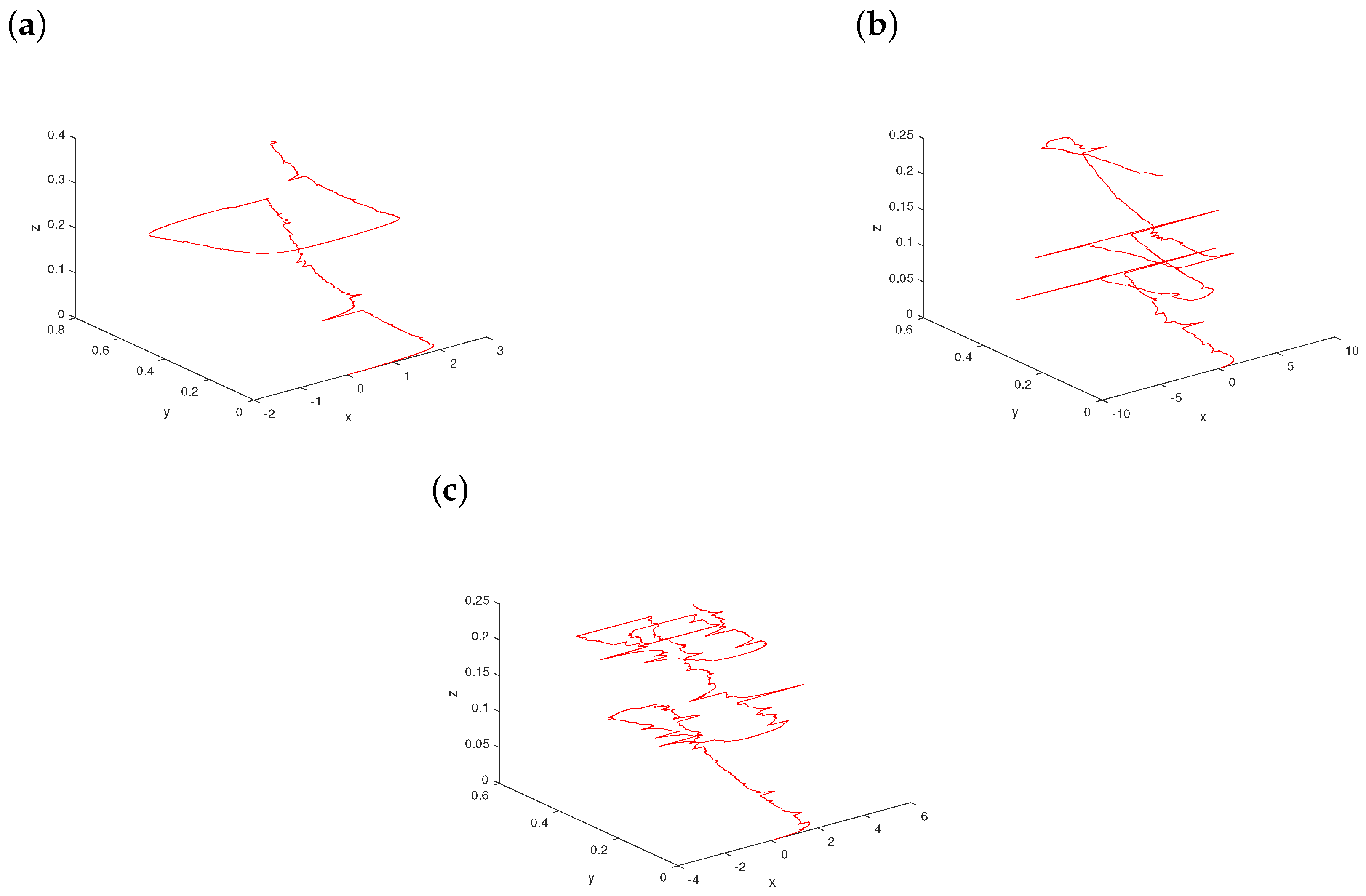
Observe that, in the beginning, the blue curve of system (8) with ϵ = 0.05 departs from x ( 0 ) = y ( 0 ) = z ( 0 ) = 0 along the direction of the x-axis, shown in Figure 1a. However, some time later, there is a gentle growing tendency for the trajectory at x ( t ) = 2 to move upward. With the increase of time, the path encounters a crucial turning point and has a precipitous climb to the stable fixed point P. More significantly, it is parallel to the ( y , z ) -plane of the slow variables in this situation. By comparison with Figure 2 and Figure 3, the Koper system (7) exhibits sensitivity to stochastic disturbance.
We sketch three time series data for the system (8) when x ( 0 ) = y ( 0 ) = z ( 0 ) = 0 and ϵ = 0.05 , as clearly detailed in Figure 1b. It manifests that the fast variable x ( t ) jumps to 2 instantaneously at first, and then decreases to 1 rapidly and suddenly. The green curve about x ( t ) stays at the same level after t = 15 . From the time series drawings of the slow variables y ( t ) and z ( t ) , they both grow to 1 eventually. The red path about y ( t ) increases much quicker than the purple trajectory about z ( t ) .
If we fix σ = 0.5 and increase α in system (7) for the choice of initial conditions x ( 0 ) = y ( 0 ) = z ( 0 ) = 0 with a scaling parameter ϵ = 0.05 , we observe the following typical sequence of events in Figure 2. The stochastic nonlinear dynamics with the stability index α = 0.8 display the complex spatio-temporal oscillations accompanied by a few big jumps as depicted in Figure 2a. With respect to α = 1.6 , the external Lévy noise leads to dramatically different dynamical behavior in the red trajectory, which is confirmed numerically in Figure 2b. As the stability index α is increased toward 1.9, the path of stochastic system (7) shows low frequency oscillations excited by Lévy noise as illustrated in Figure 2c. For three different values of α, stochastic noise of the the fast variable x can significantly influence the dynamics of the whole Koper model. However, the shapes of different trajectories from the viewpoint of the slow surface ( y , z ) are consistent.
Now, we fix α = 1 and consider a variation of σ in system (7) starting from x ( 0 ) = y ( 0 ) = z ( 0 ) = 0 with a scaling parameter ϵ = 0.05 ; see Figure 3. For small enough σ = 0.1 , the path has a spiral pattern with small-amplitude fluctuations, which is clearly demonstrated in Figure 3a. When σ-value just arrives at 0.5, the status of the path changes happens abruptly for stochastic system (7) as plotted in Figure 3b. As the noise intensity σ increases further to 0.8, large variations in the dynamics of the trajectory are indicated in Figure 3c because of strong external noise. Based on the effects of increasing noise intensities, the curves become more and more sophisticated.
The nonlocal Fokker–Planck equation [33] is a vital tool for studying the dynamical behaviors of stochastic Koper system (7). Define f : R 3 R as a smooth function. Suppose that the solution ( x , y , z ) of system (7) possesses a conditional probability density p ( x , y , z , t | x 0 , y 0 , z 0 , t ) . For simplicity in the notation, we hide the initial condition and denote it by p ( x , y , z , t ) .
We can apply an Itô formula to stochastic Koper system (7) to obtain
d f ( x , y , z ) = ϵ 1 ( x 3 + 3 x 10 y + 5 z + 3 ) x f ( x , y , z ) d t + ( x 2 y + z ) y f ( x , y , z ) d t + ( y z ) z f ( x , y , z ) d t + R { 0 } f ( x + σ ε 1 / α u , y , z ) f ( x , y , z ) σ ε 1 / α u 1 { | u | 1 } x f ( x , y , z ) ν α ( d u ) d t = [ ϵ 1 ( x 3 + 3 x 10 y + 5 z + 3 ) x f ( x , y , z ) + ( x 2 y + z ) y f ( x , y , z ) + ( y z ) z f ( x , y , z ) + σ α ε 1 R { 0 } f ( x + u , y , z ) f ( x , y , z ) ν α ( d u ) ] d t ,
where 1 { | u | 1 } stands for the indicator function of the set { | u | 1 } , ν α ( d u ) = c ( α ) 1 | u | 1 + α d z represents the α-stable Lévy measure with c α = α Γ ( 1 + α 2 ) 2 1 α π 1 2 Γ ( 1 α 2 ) , and Γ is the Gamma function [34].
If we take expectations on both sides of (9), then we have
d E f ( x , y , z ) = E [ ϵ 1 ( x 3 + 3 x 10 y + 5 z + 3 ) x f ( x , y , z ) + ( x 2 y + z ) y f ( x , y , z ) + ( y z ) z f ( x , y , z ) + σ α ε 1 R { 0 } f ( x + u , y , z ) f ( x , y , z ) ν α ( d u ) ] d t .
It is worth mentioning that the generator for system (7) is determined by
A p ( x , y , z , t ) : = ϵ 1 ( x 3 + 3 x 10 y + 5 z + 3 ) x p ( x , y , z , t ) + ( x 2 y + z ) y p ( x , y , z , t ) + ( y z ) z p ( x , y , z , t ) + σ α ε 1 R { 0 } p ( x + u , y , z , t ) p ( x , y , z , t ) ν α ( d u ) .
We are able to rewrite Equation (10) into
d d t E f ( x , y , z ) = E [ ϵ 1 ( x 3 + 3 x 10 y + 5 z + 3 ) x f ( x , y , z ) + ( x 2 y + z ) y f ( x , y , z ) + ( y z ) z f ( x , y , z ) + σ α ε 1 R { 0 } f ( x + u , y , z ) f ( x , y , z ) ν α ( d u ) ] = R 3 [ ϵ 1 ( x 3 + 3 x 10 y + 5 z + 3 ) x f ( x , y , z ) + ( x 2 y + z ) y f ( x , y , z ) + ( y z ) z f ( x , y , z ) + σ α ε 1 R { 0 } f ( x + u , y , z ) f ( x , y , z ) ν α ( d u ) ] p ( x , y , z , t ) d x d y d z = R 3 f ( x , y , z ) ( ϵ 1 x [ ( x 3 3 x + 10 y 5 z 3 ) p ( x , y , z , t ) ] y [ ( x 2 y + z ) p ( x , y , z , t ) ] z [ ( y z ) p ( x , y , z , t ) ] σ α ε 1 R { 0 } p ( x , y , z , t ) p ( x u , y , z , t ) ν α ( d u ) ) d x d y d z .
It follows that the adjoint operator of the generator A is
A * p ( x , y , z , t ) : = ϵ 1 x [ ( x 3 3 x + 10 y 5 z 3 ) p ( x , y , z , t ) ] y [ ( x 2 y + z ) p ( x , y , z , t ) ] z [ ( y z ) p ( x , y , z , t ) ] σ α ε 1 R { 0 } p ( x , y , z , t ) p ( x u , y , z , t ) ν α ( d u ) .
Furthermore, the nonlocal Fokker–Planck equation for stochastic Koper system (11) is
t p ( x , y , z , t ) = ϵ 1 x [ ( x 3 3 x + 10 y 5 z 3 ) p ( x , y , z , t ) ] y [ ( x 2 y + z ) p ( x , y , z , t ) ] z [ ( y z ) p ( x , y , z , t ) ] σ α ε 1 R { 0 } p ( x , y , z , t ) p ( x u , y , z , t ) ν α ( d u ) = ϵ 1 [ 3 ( x 2 1 ) p ( x , y , z , t ) + ( x 3 3 x + 10 y 5 z 3 ) x p ( x , y , z , t ) ] ( x 2 y + z ) y p ( x , y , z , t ) ( y z ) z p ( x , y , z , t ) + 3 p ( x , y , z , t ) + σ α ε 1 R { 0 } p ( x + u , y , z , t ) p ( x , y , z , t ) ν α ( d u )
with the initial condition p ( x , y , z , 0 ) = δ ( x x 0 , y y 0 , z z 0 ) .
Considering a variation of λ ( z ) and fix k = 10 , stochastic Hopf bifurcation occurs for λ ( z ) 7.67 . Numerical simulations always give a clear insight into how the trajectories develop for various values of λ ( z ) . However, stochastic modeling of slow manifold is much more complicated owing to the dependent integrals of the Lévy noise. Fortunately, the projections in the slow coordinates are useful in forecasting and suggesting stochastic dynamics.
Example 2.
Now, we proceed to analyze the stochastic system
x ˙ = 1 ϵ ( x 3 + 3 x 10 y 7 ) + σ ϵ α L ˙ t α , i n   R y ˙ = x 2 y + z , i n   R z ˙ = y z , i n   R
where x is the “fast" component, ( y , z ) is the “slow" component, and λ ( z ) = 7 .
Due to the time scaling t ϵ t and the self-similarity ϵ 1 / α L ϵ t α = d L t α , stochastic Koper system (11) in the sense of distribution is equivalent to
d x = ( x 3 + 3 x 10 y 7 ) d t + σ d L t α , i n   R d y = ϵ ( x 2 y + z ) d t , i n   R d z = ϵ ( y z ) d t , i n   R
As a consequence of σ = 0 , we derive the deterministic system displaying quasi-periodicity
x ˙ = ( x 3 + 3 x 10 y 7 ) , i n   R y ˙ = ϵ ( x 2 y + z ) , i n   R z ˙ = ϵ ( y z ) , i n   R
As seen in Figure 4a, there is a rich variety of dynamics which can be plotted in three-dimensional space. For one set of initial conditions x ( 0 ) = y ( 0 ) = z ( 0 ) = 0 , the blue trajectory of the solution ( x ( t ) , y ( t ) , z ( t ) ) of system (12) turns around exponentially, and moves closer and closer to the fold curve in finite time. The three variables x ( t ) , y ( t ) , and z ( t ) coexist and oscillate in phase. There are three distinct amplitudes with respect to x ( t ) , y ( t ) , and z ( t ) . The shapes have discrete peaks displaying the quasiperiodic behaviors. The results are summarized in Figure 4b.
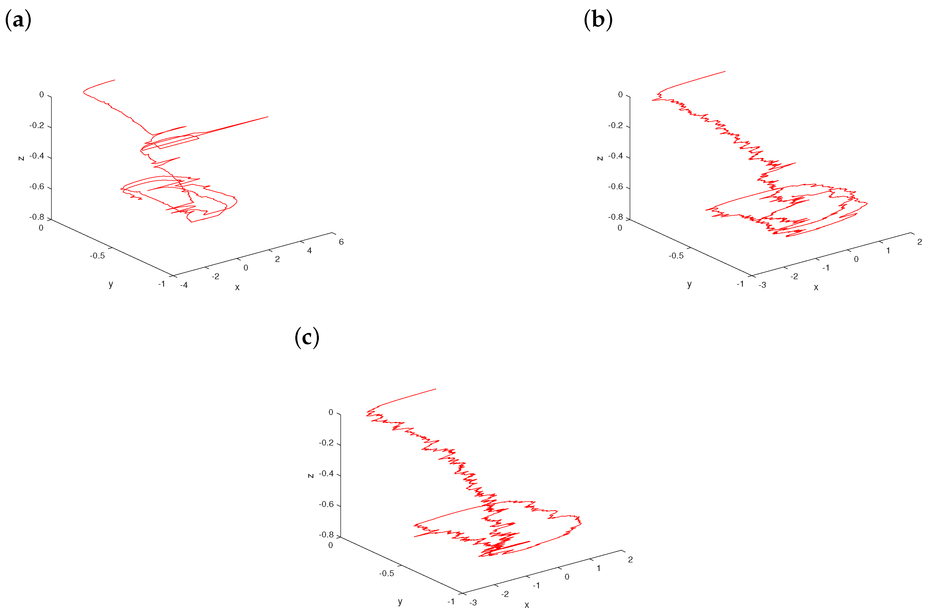
It can be discerned from Figure 5a that the intermittency is present in the path of stochastic Koper system (11) with α = 0.8 , which can lead to extremely complex random behavior. When α = 1.6 , the trajectory of system (11) goes through a stochastic regime with an irregular pattern observed in Figure 5b. As the stability index gets large, system (11) forced with noise is structurally unstable. The quasiperiodic behavior is interrupted by occasional stochastic bursts. This complication is confirmed in Figure 5c for α = 1.9 .
It is clearly seen in Figure 6a that the path displays what appears to be random behavior with small noise intensity σ = 0.1 . As systematically captured in Figure 6b, the trajectory of system (11) could be depicting a very high stochasticity when σ = 0.5 . The aperiodic random behavior of system (11) can be evidently detected in Figure 6c, if there is noisy input with σ = 0.8 . Comparing the results with the deterministic system (12), there is no quasiperiodic behavior in stochastic Koper system (11).
Moreover, the nonlocal Fokker–Planck equation for stochastic Koper system (11) is
t p ( x , y , z , t ) = ϵ 1 x [ ( x 3 3 x + 10 y + 7 ) p ( x , y , z , t ) ] y [ ( x 2 y + z ) p ( x , y , z , t ) ] z [ ( y z ) p ( x , y , z , t ) ] σ α ε 1 R { 0 } p ( x , y , z , t ) p ( x u , y , z , t ) ν α ( d u ) = ϵ 1 [ 3 ( x 2 1 ) p ( x , y , z , t ) + ( x 3 3 x + 10 y + 7 ) x p ( x , y , z , t ) ] ( x 2 y + z ) y p ( x , y , z , t ) ( y z ) z p ( x , y , z , t ) + 3 p ( x , y , z , t ) + σ α ε 1 R { 0 } p ( x + u , y , z , t ) p ( x , y , z , t ) ν α ( d u )
with the initial condition p ( x , y , z , 0 ) = δ ( x x 0 , y y 0 , z z 0 ) .

6. Conclusions and Future Challenges

We investigated three-dimensional stochastic slow-fast Koper system (1) driven by α -stable Lévy noise, and proved that stochastic slow manifolds exist. We constructed the slow manifold in which the fast variable x can be expressed as the random function of the two slow variables y and z. Stochastic nonlinear dimensionality reduction helped us make more accurate predictions by using stochastic differential equations for the slow variables. We carried out the computation of the practical Koper models (7)–(8) and (11)–(12). Compared with the reference [20], we probed the orbital dynamics of stochastic Koper systems to provide a better understanding of underlying and fascinating properties, and also perceived stochastic Hopf bifurcation for noisy Koper dynamical systems. In addition, we rigorously calculated the conditional probability density described by the nonlocal Fokker–Planck equation.
When the scaling parameter ϵ ^ is sufficiently small, i.e., 0 < ϵ ^ 1 , stochastic Koper model (1) has three times scales: variable x is fast, y is slow, and z is slower. It indicates the ratio of three times scales such that | d x d t | | d y d t | | d z d t | . Thus, it is meaningful to project high-dimensional dynamics onto lower-dimensional effective manifolds in this case.
What happens if the main bifurcation parameters k and λ ( z ) = : λ change? The folded node/focus and supercritical Hopf bifurcation are expected to occur in parameter space for the Koper model without noise. By classifying the type and stability of the equilibrium points, we obtain a bifurcation diagram under parameter variation.
We can generalize the consideration to a number of cases where the variables x, y, and z both are perturbed by α -stable Lévy noises, even to the extent that the influences are the more general Lévy processes including multiplicative and additive effects. We may use Itô, Stratonovich, or Marcus type stochastic differential equations.
The orbits can escape from the region of the metastable equilibrium if we face random perturbation [35]. It is interesting to characterize the most probable transition from one metastable state to another [36,37]. The random slow manifold still depends on k and λ . It is a challenge to plot the bifurcation diagram in the ( k , λ ) -plane of the random slow flow. Luckily, we can explore stochastic bifurcations in dynamical systems driven by Lévy noises with support for statistical modeling and computation [18,19,38].
We often have difficulty comprehending data in phase space with the attracting or repelling of random slow manifolds. Thus, it is useful for visualization purposes in order to reduce data to a small number of dimensions.

Author Contributions

Writing—original draft, H.Z.; Writing—review & editing and Software, S.Y.; Supervision, M.S.S. All authors have read and agreed to the published version of the manuscript.

Funding

The authors acknowledge support from the NSFC grant 12001213.

Institutional Review Board Statement

Not applicable.

Informed Consent Statement

Not applicable.

Data Availability Statement

Numerical algorithms’ source code that supports the findings of this study are openly available in GitHub [39].

Acknowledgments

The authors express their gratitude to the editors and the reviewers for the thoughtful comments, which considerably improved the presentation of this paper.

Conflicts of Interest

The authors declare that they have no conflict of interest.

References

  1. Koper, M.T.M. Bifurcations of mixed-mode oscillations in a three-variable autonomous Van der Pol-Duffing model with a cross-shaped phase diagram. Phys. D 1995, 80, 72–94. [Google Scholar] [CrossRef]
  2. Balabaev, M. Invariant manifold of variable stability in the Koper model. J. Phys. Conf. Ser. 2019, 1368, 042003. [Google Scholar] [CrossRef]
  3. Bates, P.W.; Lu, K.; Zeng, C. Existence and Persistence of Invariant Manifolds for Semiflows in Banach Space; American Mathematical Society: Providence, RI, USA, 1998. [Google Scholar]
  4. Henry, D. Geometric Theory of Semilinear Parabolic Equations; Springer: Berlin/Heidelberg, Germany, 2006. [Google Scholar]
  5. Chicone, C.; Latushkin, Y. Center manifolds for infinite dimensional nonautonomous differential equations. J. Differ. Equ. 1997, 141, 356–399. [Google Scholar] [CrossRef] [Green Version]
  6. Chow, S.N.; Lu, K.; Lin, X.B. Smooth foliations for flows in Banach space. J. Differ. Equ. 1991, 94, 266–291. [Google Scholar] [CrossRef] [Green Version]
  7. Ruelle, D. Characteristic exponents and invariant manifolds in Hilbert space. Ann. Math. 1982, 115, 243–290. [Google Scholar] [CrossRef]
  8. Caraballo, T.; Chueshov, I.; Langa, J.A. Existence of invariant manifolds for coupled parabolic and hyperbolic stochastic partial differential equations. Nonlinearity 2005, 18, 747–767. [Google Scholar] [CrossRef]
  9. Chow, S.N.; Lu, K. Invariant manifolds for flows in Banach spaces. J. Differ. Equ. 1988, 74, 285–317. [Google Scholar] [CrossRef] [Green Version]
  10. Yuan, S.; Li, Y.; Zeng, Z. Stochastic bifurcations and tipping phenomena of insect outbreak systems driven by α-stable Lévy processes. Math. Model. Nat. Phenom. 2022, 17, 34. [Google Scholar] [CrossRef]
  11. Fu, H.; Liu, X.; Duan, J. Slow manifolds for multi-time-scale stochastic evolutionary systems. Comm. Math. Sci. 2013, 11, 141–162. [Google Scholar]
  12. Schmalfuss, B.; Schneider, K.R. Invariant manifolds for random dynamical systems with slow and fast variables. J. Dyn. Differ. Equ. 2008, 20, 133–164. [Google Scholar] [CrossRef]
  13. Wang, W.; Roberts, A. Slow manifold and averaging for slow-fast stochastic differential system. J. Math. Anal. Appl. 2013, 398, 822–839. [Google Scholar] [CrossRef]
  14. Ren, J.; Duan, J.; Jones, C.K.R.T. Approximation of random slow manifolds and settling of inertial particles under uncertainty. J. Dyn. Differ. Equ. 2015, 27, 961–979. [Google Scholar] [CrossRef] [Green Version]
  15. Ren, J.; Duan, J.; Wang, X. A parameter estimation method based on random slow manifolds. Appl. Math. Model. 2015, 39, 3721–3732. [Google Scholar] [CrossRef]
  16. Yuan, S.; Blömker, D.; Duan, J. Stochastic turbulence for Burgers equation driven by cylindrical Lévy process. Stoch. Dynam. 2022, 22, 2240004. [Google Scholar] [CrossRef]
  17. Qiao, M.; Yuan, S. Analysis of a stochastic predator-prey model with prey subject to disease and Lévy noise. Stochastics Dyn. 2019, 19, 1950038. [Google Scholar] [CrossRef]
  18. Yuan, S.; Blömker, D. Modulation and amplitude equations on bounded domains for nonlinear SPDEs driven by cylindrical α-stable Lévy processes. SIAM J. Appl. Dyn. Syst. 2022, 21, 1748–1777. [Google Scholar] [CrossRef]
  19. Yuan, S.; Zeng, Z.; Duan, J. Stochastic bifurcation for two-time-scale dynamical system with α-stable Lévy noise. J. Stat. Mech. 2021, 2021, 033204. [Google Scholar] [CrossRef]
  20. Yuan, S.; Hu, J.; Liu, X.; Duan, J. Slow manifolds for dynamical systems with non-Gaussian stable Lévy noise. Anal. Appl. 2019, 17, 477–511. [Google Scholar] [CrossRef]
  21. Zulfiqar, H.; He, Z.; Yang, M.; Duan, J. Slow manifold and parameter estimation for a nonlocal fast-slow dynamical system with brownian motion. Acta Math. Sci. 2021, 41, 1057–1080. [Google Scholar] [CrossRef]
  22. Zulfiqar, H.; Yuan, S.; He, Z.; Duan, J. Slow manifolds for a nonlocal fast-slow stochastic system with stable Lévy noise. J. Math. Phys. 2019, 60, 091501. [Google Scholar] [CrossRef]
  23. Applebaum, D. Lévy Processes and Stochastic Calculus; Cambridge University Press: Cambridge, UK, 2009. [Google Scholar]
  24. Duan, J.; Lu, K.; Schmalfuss, B. Smooth stable and unstable manifolds for stochastic evolutionary equations. J. Dyn. Differ. Equ. 2004, 16, 949–972. [Google Scholar] [CrossRef] [Green Version]
  25. Chao, Y.; Wei, P.; Yuan, S. Invariant foliations for stochastic dynamical systems with multiplicative stable Lévy noise. Electron. J. Differ. Equ. 2019, 2019, 1–21. [Google Scholar]
  26. Wei, H.H. Weak convergence of probability measures on metric spaces of nonlinear operators. Bull. Inst. Math. Acad. Sin. 2016, 11, 485–519. [Google Scholar] [CrossRef] [Green Version]
  27. Arnold, L. Random Dynamical Systems; Springer: Berlin/Heidelberg, Germany, 2013. [Google Scholar]
  28. Duan, J. An Introduction to Stochastic Dynamics; Cambridge University Press: Cambridge, UK, 2015. [Google Scholar]
  29. Protter, P. Stochastic Integration and Differential Equations; Springer: Berlin/Heidelberg, Germany, 2004. [Google Scholar]
  30. Yang, X.; Xu, Y.; Wang, R.; Jiao, Z. The central limit theorem for slow-fast systems with Lévy noise. Appl. Math. Lett. 2022, 128, 107897. [Google Scholar] [CrossRef]
  31. Jacod, J.; Shiryaev, A. Limit Theorems for Stochastic Processes; Springer: Berlin/Heidelberg, Germany, 2013. [Google Scholar]
  32. Castaing, C.; Valadier, M. Convex Analysis and Measurable Multifunctions; Springer: Berlin/Heidelberg, Germany, 2006. [Google Scholar]
  33. Moradi, S.; del-Castillo-Negrete, D.; Anderson, J. Charged particle dynamics in the presence of non-Gaussian Lévy electrostatic fluctuations. Phys. Plasmas 2016, 23, 090704. [Google Scholar] [CrossRef] [Green Version]
  34. Yuan, S.; Wang, Z. Bifurcation and chaotic behaviour in stochastic Rosenzweig-MacArthur prey-predator model with non-Gaussian stable Lévy noise. Int. J. Non-Linear Mech. 2023, 150, 104339. [Google Scholar] [CrossRef]
  35. Li, Y.; Yuan, S.; Xu, S. Controlling mean exit time of stochastic dynamical systems based on quasipotential and machine learning. arXiv 2022, arXiv:2209.13098.2006. [Google Scholar] [CrossRef]
  36. Huang, Y.; Chao, Y.; Yuan, S.; Duan, J. Characterization of the most probable transition paths of stochastic dynamical systems with stable Lévy noise. J. Math. Phys. 2019, 2019, 063204. [Google Scholar] [CrossRef] [Green Version]
  37. Tesfay, A.; Yuan, S.; Tesfay, D.; Brannan, J. Most Probable Dynamics of the Single-Species with Allee Effect under Jump-diffusion Noise. arXiv 2021, arXiv:2112.07234. [Google Scholar]
  38. Tesfay, A.; Tesfay, D.; Yuan, S.; Brannan, J.; Duan, J. Stochastic bifurcation in single-species model induced by α-stable Lévy noise. J. Stat. Mech. 2021, 2021, 103403. [Google Scholar] [CrossRef]
  39. Yuan, S. Code. Github. 2022. Available online: https://github.com/ShenglanYuan/Slow-manifolds-for-stochastic-Koper-models-with-stable-L-vy-noises (accessed on 7 December 2022).
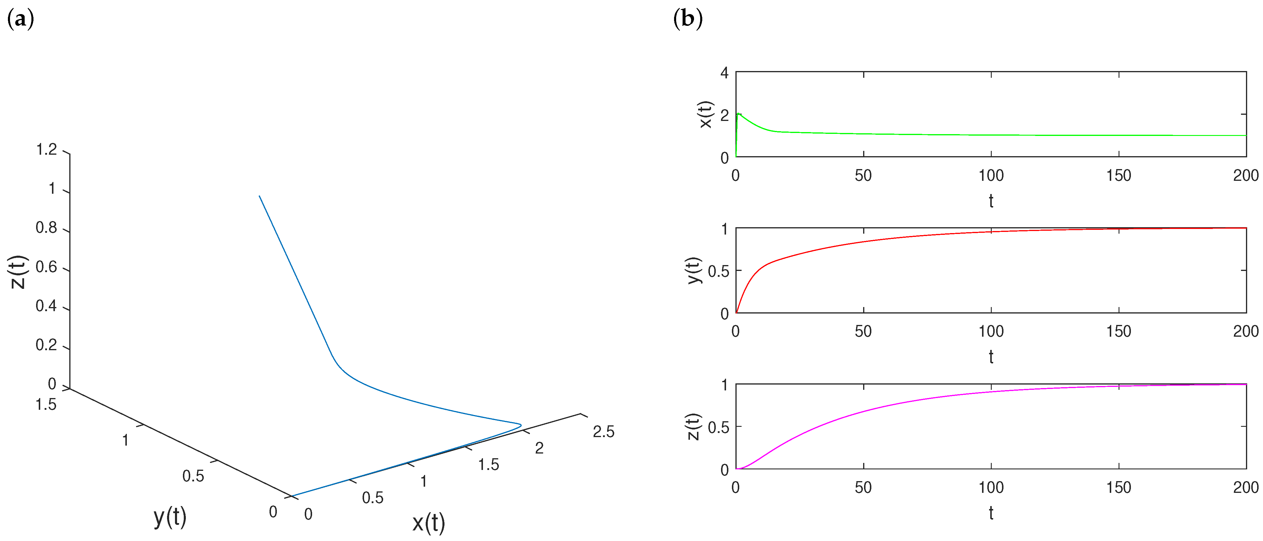
Figure 1. When x ( 0 ) = y ( 0 ) = z ( 0 ) = 0 and ϵ = 0.05 : (a) dynamical behavior for the trajectory of system (8); (b) the three variables x ( t ) , y ( t ) , and z ( t ) in system (8) eventually settle down to constant values.
Axioms 12 00261 g001
Figure 2. The evolution of system (7) for the choice of initial conditions x ( 0 ) = y ( 0 ) = z ( 0 ) = 0 at the fixed noise intensity σ = 0.5 with a scaling parameter ϵ = 0.05 and a gradual increase in the stability index: (a) α = 0.8 ; (b) α = 1.6 ; (c) α = 1.9 .
Axioms 12 00261 g002
Figure 3. The evolution of system (7) starting from x ( 0 ) = y ( 0 ) = z ( 0 ) = 0 with a fixed stability index α = 1 and a scaling parameter ϵ = 0.05 as the noise intensity increases: (a) σ = 0.1 ; (b) σ = 0.5 ; (c) σ = 0.8 .
Axioms 12 00261 g003
Figure 4. When x ( 0 ) = y ( 0 ) = z ( 0 ) = 0 and ϵ = 0.1 : (a) dynamical trajectory of system (12); (b) quasiperiodic behaviors for the three variables x ( t ) , y ( t ) , and z ( t ) in system (12).
Axioms 12 00261 g004
Figure 5. The evolution of system (11) for the choice of initial conditions x ( 0 ) = y ( 0 ) = z ( 0 ) = 0 at the fixed noise intensity σ = 0.5 with a scaling parameter ϵ = 0.1 and a gradual increase in the stability index: (a) α = 0.8 ; (b) α = 1.6 ; (c) α = 1.9 .
Axioms 12 00261 g005
Figure 6. The evolution of system (11) for one set of initial conditions x ( 0 ) = y ( 0 ) = z ( 0 ) = 0 with a fixed stability index α = 1 and a scaling parameter ϵ = 0.1 as the noise intensity increases: (a) σ = 0.1 ; (b) σ = 0.5 ; (c) σ = 0.8 .
Axioms 12 00261 g006
Disclaimer/Publisher’s Note: The statements, opinions and data contained in all publications are solely those of the individual author(s) and contributor(s) and not of MDPI and/or the editor(s). MDPI and/or the editor(s) disclaim responsibility for any injury to people or property resulting from any ideas, methods, instructions or products referred to in the content.