Abstract
The Shanker distribution, a one-parameter lifetime distribution with an increasing hazard rate function, is recommended by Shanker for modelling lifespan data. In this study, we examine the theoretical and practical implications of 2-component mixture of Shanker model (2-CMSM). A significant feature of proposed model’s hazard rate function is that it has rising, decreasing, and upside-down bathtub forms. We investigate the statistical characteristics of a mixed model, such as the probability-generating function, the factorial-moment-generating function, cumulants, the characteristic function, the Mills ratio, the mean residual life, and the mean time to failure. There is a graphic representation of density, mean, hazard rate functions, coefficient of variation, skewness, and kurtosis. Our final approach is to estimate the parameters of the mixture model using appropriate approaches such as maximum likelihood, least squares, and weighted least squares. Using a simulation analysis, we examined how the estimates behaved graphically. The simulation results demonstrated that, in the majority of cases, the maximum likelihood estimates have the smallest mean square errors among all other estimates. Finally, we observed that when the sample size rises, the precision measures decrease for all of the estimation techniques, indicating that all of the estimation approaches are consistent. Through two real data analyses, the suggested model’s validity and adaptability are contrasted with those of other models, including the mixture of the exponential distributions and the Lindley distributions .
Keywords:
least square estimation (LSE); mixture distributions; Mills ratio; weighted least square estimation MSC:
60E05; 62E15; 62E05; 62F10
1. Introduction
Mixture models, more specifically finite-mixture models, have been used more frequently over time to simulate a wider range of events than they were in the early days of statistics. Available data can often be thought of as a mixture of two or more models. Utilizing this concept, we can combine statistical distributions to produce a novel one. The fields of biology, genetics, engineering, medicine, marketing, business, real-world applications, and social sciences are just a few that can benefit from the use of finite-mixture distributions. In mixture distributions, two or more distributions are combined by adjusting the proportions to form a novel model. Therefore, it is essential to look into the statistical characteristics of the suggested mixture distribution and apply the right techniques to estimate its unknown parameters. Several authors have examined mixing distributions, including [1,2,3,4,5]. Muhammad and Muhammad [6] examined the traditional features of mixture of the Burr XII and Weibull distribution. A two-component mixture of inverse Weibull distribution (2-CMIWD) was proposed by Sultan et al. [7], and some of its characteristics were investigated by utilizing density and hazard function graphs. Jiang et al. [8] focused on the graphical approaches as well as the PDF and hrfs formats to analyze the hybrid of two inverse Weibull distributions. Several authors who address mixture modelling in various real-world issues include those listed below: Mohamed et al. [9], Mohammadi et al. [10], Ateya [11], and Sindhu et al. [12] are a few examples. The generalized method of moments and ML were employed by Al-Moisheer et al. [13] to assess the mixture model’s unknown parameters. Some other relevant studies are [14,15,16,17,18,19,20].
Shanker [21] proposed the Shanker distribution as a lifetime distribution and estimated its parameter by employing maximum likelihood estimation and moments methodology, as well as by employing those models on how we can model lifetime data from the field of medical science and engineering. The discrete Poisson-Shanker model was developed by Shanker [22], who also studied its mathematical and statistical properties as well as potential uses for count data from many fields of study. In [23], the authors conducted a comparison analysis on modelling lifespan data utilizing one parameter Akash, exponential, and Lindley models, finding that the Akash model of Shanker has flexibility over both exponential and Lindley models. Shanker et al. [24] conducted a thorough comparison of exponential and Lindley models for modelling diverse real-life data sets and discovered that in certain cases, Lindley is superior to exponential, while in others, exponential is superior to Lindley.
The maximal likelihood estimation (MLE) is a well-known estimation approach. Despite the fact that MLE is efficient and has good theoretical features, there is evidence that it does not perform effectively, particularly with small samples. As a result, different estimation approaches have been offered in the literature as alternatives to the conventional method. The weighted least-squares estimation (WLSE), least squares estimator (LSE), L-moments estimator (LME), and percentile estimator (PCE) are among the most frequently recommended. These approaches, in general, do not have good theoretical properties, but they can offer better estimates of unknown parameters in specific instances compared to the MLE. The literature has investigated a variety of estimating techniques for different distributions, such as [25,26,27,28,29,30]. The aim of the current study is to provide professional statisticians with a framework for choosing the best estimation methodology for 2-component Mixtures of Shanker Models (2-CMSM). This study uses weighted least square estimation (WLSE), least square estimation (LSE) in addition to MLE for estimating the 2-component mixture of the Shanker model (2-CMSM).
Our goal in this study is to develop a distribution for modelling real lifespan data sets from various disciplines of knowledge that are better fitting than both exponential and Lindley distributions. The mixture of the Shanker distribution has one advantage over the one-component Shanker and the exponential distribution: that the Shanker distribution has an increasing, while exponential distribution has constant, hazard rate, whereas the mixture of the Shanker model has decreasing, increasing, rising-decreasing, constant, unimodal, and “upside-down” bathtub curve failure rates .
The 2-CMSM is being developed for analyzing complex data arising from reliability research, survival analysis, statistical mechanics, quality control, economics, biological investigations, and other fields. Our aim is to develop this distribution because of the different shapes of hazard function, including the increasing, decreasing, unimodal, and upside-down bathtub curve, as well as various close-form features of 2-CMSM with simple physical explanations. The originality of this study stems from a comprehensive explanation of mathematical and statistical features of this model, which will hopefully attract more applications in lifespan analysis. Additionally, to our knowledge, no attempt has been made to compare any of these estimating approaches to estimate parameters of 2-CMSM. For a set of parametric values and sample sizes, we illustrate the efficiency of these estimation techniques.
The rest of article is formatted as displayed. We present 2-CMSM in Section 2. In Section 3, we endeavor to derive the 2-CMSM model’s key mathematical and statistical characteristics. In Section 4, we extract some of its general reliability characteristics, such as the cumulative-hazard-rate function, the Mills ratio, the mean time to failure, and the mean residual life. In Section 5, the model pertinent parameters are estimated with LSE, MLE, and WLSE and present simulation outcomes to assess the performance of these estimators in Section 6. In Section 7, we show an application to demonstrate the mixing model’s applicability. The conclusion can be found in Section 8.
2. 2-Component Mixture of Shanker Model (2-CMSM)
A T is considered to have a finite mixture of 2-component Shanker model (2-CMSM) as its CDF and PDF can be written as:
and
where are the scale, whereas is the mixing parameter.
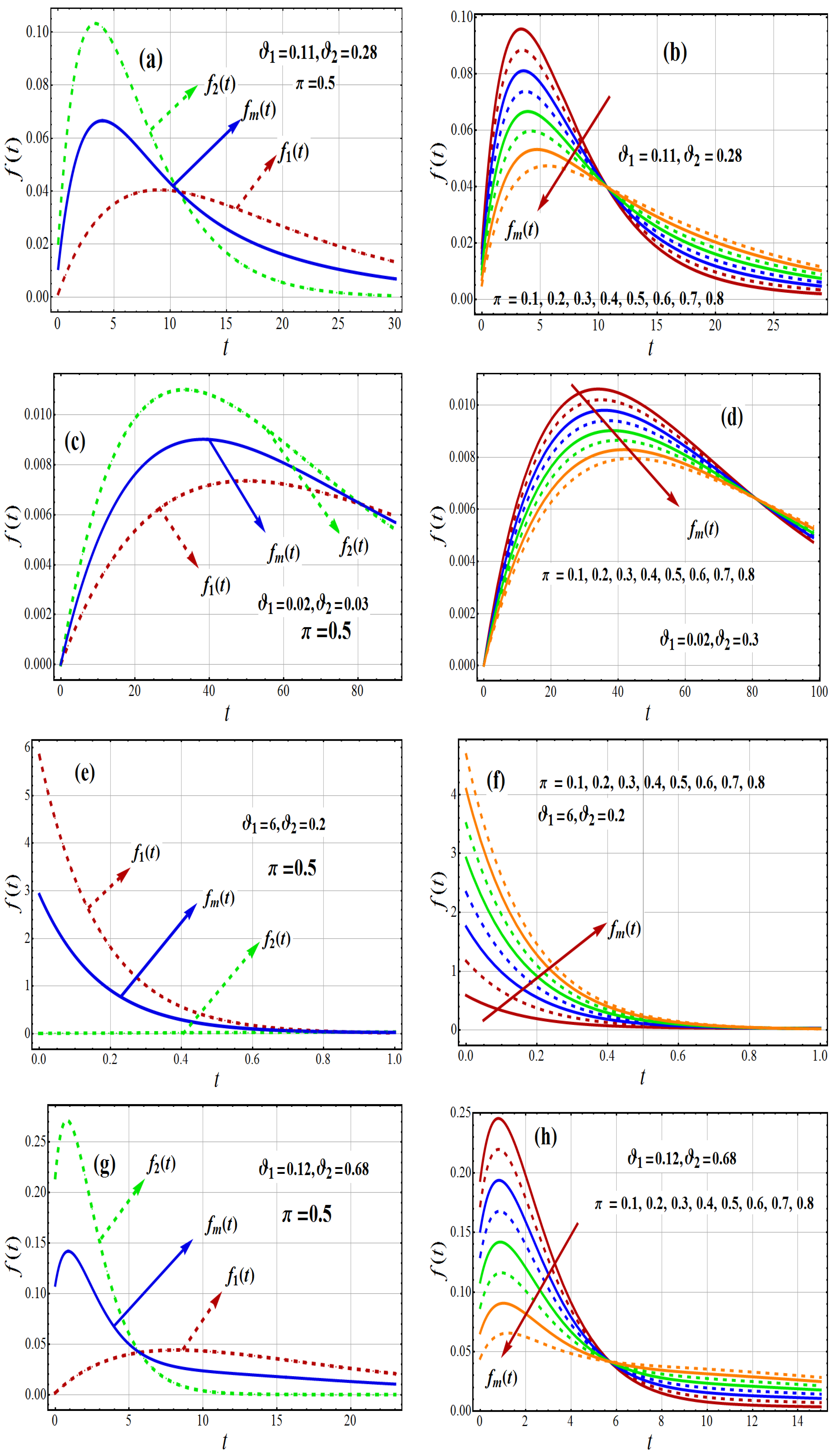
Figure 1a–h displays a number of graphs of and both component densities for different parameter values. The PDF mentioned above shows how the parametric vector affects the density of 2-CMSM(). The PDF curves of 2-CMSM() shows that it takes several shapes, such as monotonically decreasing, positively skewed, and inverted U with platykurtic, mesokurtic, and leptokurtic curves. This indicates that it can be used to model data of diverse types.
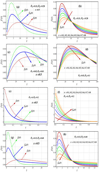
Figure 1.
Variations of first and second component of density , respectively, and density of 2-CMSM .
Identifiability
Identifiability is a condition that a statistical model must satisfy for precise inference to be possible. A model is considered identifiable if the true values of its underlying parameters can be learned after an infinite number of observations. It can be seen mathematically as an assertion that different values of the parameters will generate different probabilities of observable variables. Models are usually only identifiable under certain technical conditions, referred to as identification conditions.
Definition 1.
Let be a statistical Shanker model with parameter space . We state that f is said to be identifiable if the mapping is one-to-one:
This means that distinct values of should correspond to distinct probability models: if , then also .
By using this approach, we prove the following proposition.
Proposition 1.
The class of all finite mixing models relative to Shanker distribution is identifiable.
Let f be the pdf of statistical Shanker model:
Taking log on both sides
This expression is equal to zero for almost all t only when all its coefficients are equal to zero.
hence the identifiability is proved.
3. Statistical and Mathematical Characteristics
3.1. Mode
The nonlinear equation w.r.t. t is solved to provide the mode of the 2-CMSM:
3.2. Median
Here, we study about median of 2-CMSM. Assume that is the CDF of 2-CMSM model at 0.5th quantiles . The median () can then be obtained by resolving the following non-linear equation for t.
Computing techniques such as the Newton-Raphson methods can be used to obtain the median, , from Equation (9).
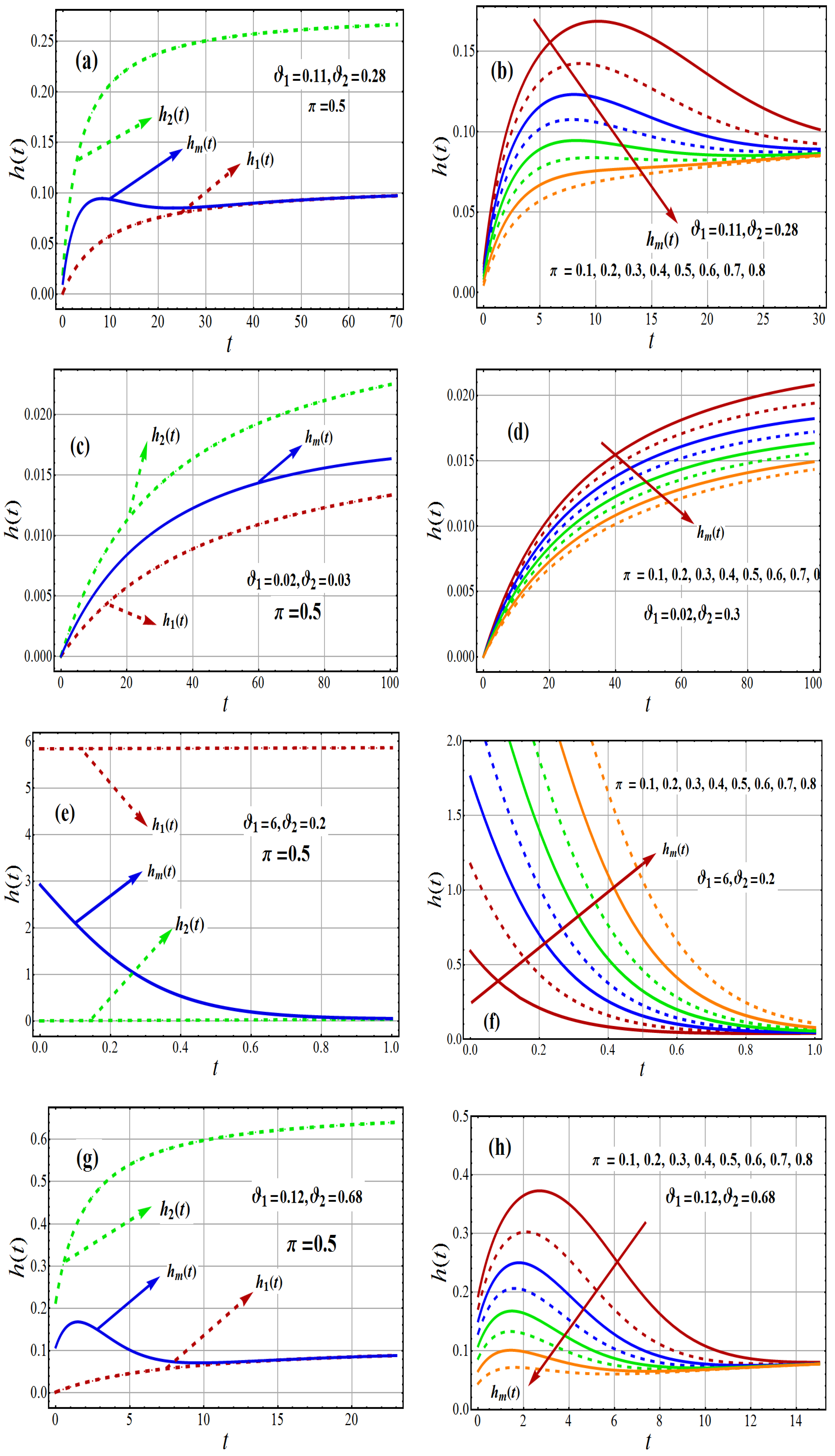
Figure 2a–h shows various graphs of hrf of one and 2-CMSM for various parameter values. It should be observed that the parameter values were chosen at random until different shapes could be obtained. An increasing trend can be seen in the hrf of each component distribution, while the hrf of 2-CMSM() shows a monotonically increasing, decreasing, upside-down bathtub, increasing decreasing-constant (IDC) behavior as shown in the figure . The hazard rate function of the 2-CMSM() highlights its versatility over one component distribution of Shanker, exponential, and Lindley, and two components of the mixture of exponential and Lindley distributions. These Figures indicate the flexibility of the 2-CMSM() distribution to model right skewed data as well as the data with decreasing and upside-down bathtub shapes.
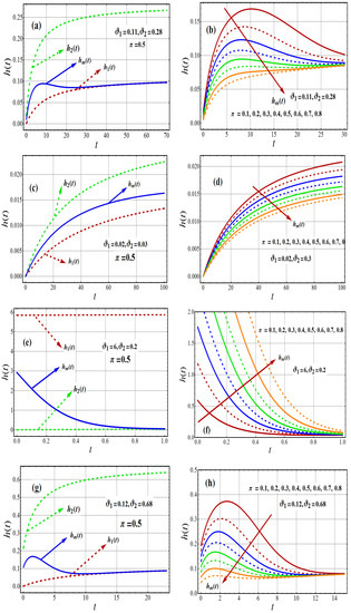
Figure 2.
Influences of first and second components hrf and hrf of 2-CMSM ).
Figure 3a–c shows the curves of the mean of 2-CMSM () for different parametric values. The mean of 2-CMSM () shows a monotonically increasing and decreasing-constant (DC) pattern. For the fixed value of and varying values of and , the mean decreases (see Figure 3a,c), whereas for the fixed value of , the mean is the increasing function of and (see Figure 3b).

Figure 3.
Variations of Mean of 2-CMSM.
3.3. Moments about Origin
The mth moments about the origin of a 2-CMSM for the random variable T are as follows:
The mean of the PDF of the 2-CMSM is:
while the variance is given by
Particularly, in the first four moments of origin
and the moments about mean of the 2-CMSM are:
The coefficient of variation , the skewness , and the Kurtosis of the 2-CMSM are:
and the index of dispersion is
The 2-CMSM distribution is simply demonstrated to be over-dispersed when , equi-dispersed as well as under-dispersed
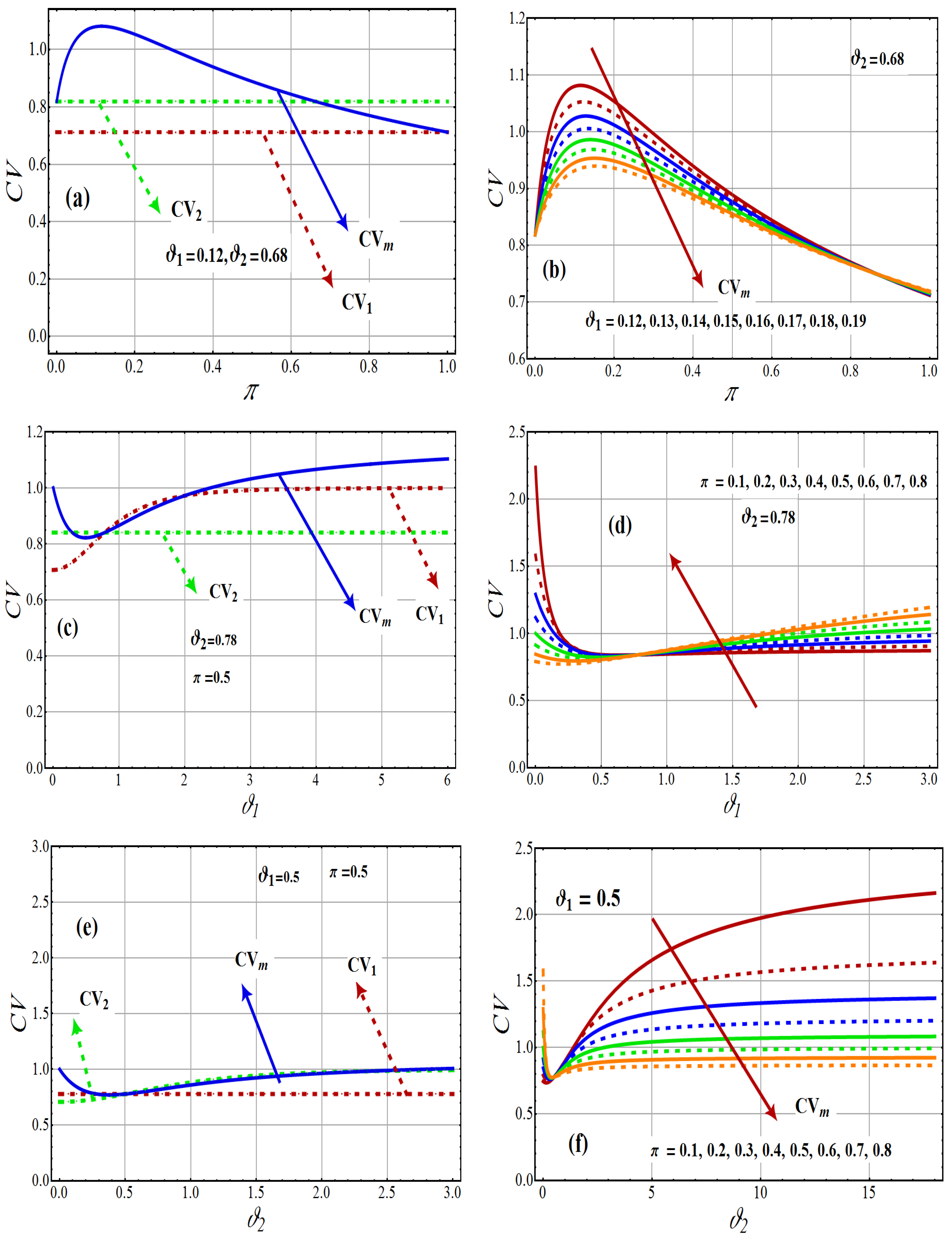
Figure 4 displays the coefficient of variation of 2-CMSM() graphs for different parametric values. Every component distribution’s coefficient of variation rises and is constant as the coefficient of variation of 2-CMSM() shows monotonically decreasing and increasing behavior. For the fixed value of and the varying values of and , the mean increases (see Figure 4b,d), whereas for the fixed value of , the mean is the decreasing function of and (see Figure 4f).
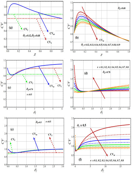
Figure 4.
Variations of coefficient of variation, for first component (CV), for second component (CV), and for 2-CMSM (CV).
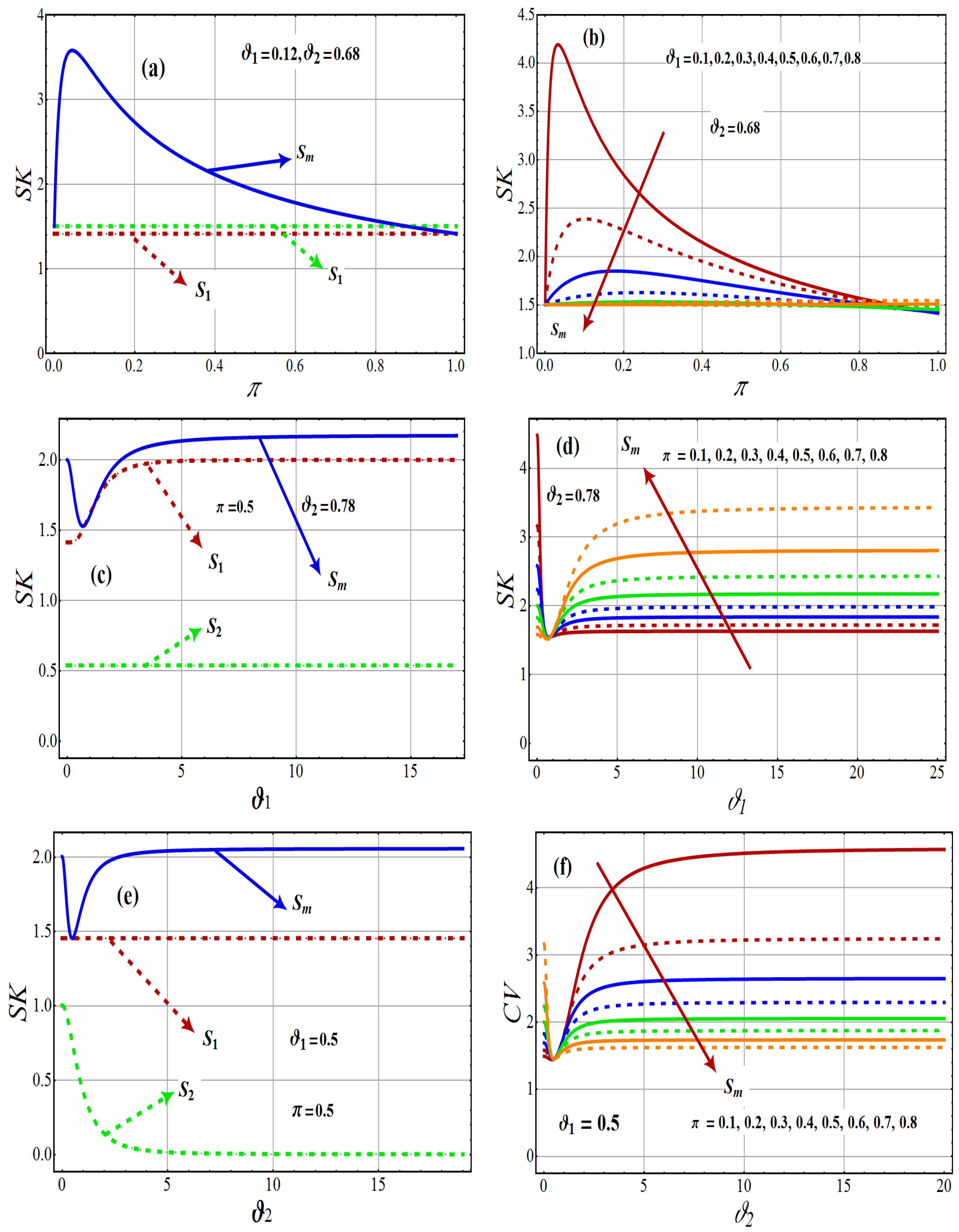
Figure 5 depicts the graphs of the skewness of one component distribution and the 2-CMSM() for various parametric values. As noted in Figure 5, the skewness of each component model grows, decreases, and is constant, whereas the skewness for 2-CMSM() increases the function under different scenarios. The behavior of Kurtosis under different scenarios is observed in Figure 6, which shows, for the fixed value of and the varying values of and , that Kurtosis increases (see Figure 6a,b), whereas for the fixed value of , Kurtosis is a decreasing function of and (see Figure 6c).
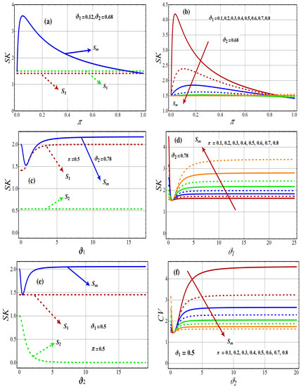
Figure 5.
Variations of coefficient of skewness, for first component (), for second component (), and for 2-CMSM ().

Figure 6.
Variations of coefficient of kurtosis , for 2-CMSM.
3.4. Moment Generating Function
The 2-CMSM’s MGF is specified as:
3.5. Cumulants
The characteristic function (CF), of 2-CMSM is obtained by putting with `’ in Equation (22); CF is obtained as
where is the complex unit.
3.6. Cumulant Generating Function
The CGF is
3.7. Probability-Generating Function
In Equation (22), we may obtain the PGF by substituting with “ln()” as shown below:
3.8. Factorial-Moment-Generating Function
The FMGF can be calculated by substituting with `ln’ in Equation (22)
4. Reliability Measures
In reliability theory, lifespan models are categorized using the reliability function and failure rate. A ratio of the lifespan model to the reliability function is the hazard rate function. An item or component with a lower dependability value will have a shorter lifespan, which means a higher hazard rate and a greater likelihood of failure. In contrast, a lower hazard rate indicates a better reliability function value, which reduces the danger of failure. The reliability characteristics of 2-CMSM are currently being explored.
4.1. Reliability Function
The reliability function of 2-CMSM is
4.2. Hazard Function
The hazard rate function of 2-CMSM is described as follows:
4.3. Mills Ratio
The Mills ratio approaches reliability in a unique way because of its relationship to failure rates.
4.4. Cumulative Hazard Rate Function
The CHRF of 2-CMSM is
It serves as a risk indicator, with a larger value indicating a greater chance of failure by time. It is observed that
Therefore,
4.5. Reversed-Hazard-Rate Function
The ratio of life likelihood function to its distribution function represents the reversed hazard rate for a random life.
4.6. Mean Time to Failure
The MTTF provides information about the anticipated (or average) period of time during which a device performs satisfactorily. If 2-CMSM, the reliability function is used to express MTTF and looks like this:
where is given in Equation (28). Hence,
4.7. Mean Residual Life
The MRL has been investigated by reliability experts, statisticians, and survival analysts, among other disciplines. It has produced a lot of beneficial outcomes. The residual lifetime after t for a system or component of age t is random. It is known as the mean residual lifetime or mean remaining life , and it is calculated as follows:
where is given in Equation (28).
5. Estimation Inference via Simulation
This section contributes a number of statistical properties of the 2-CMSM, taking into account that the parametric vector is unknown. Three widely used estimation techniques (maximum likelihood estimation, least squares estimation, and weighted least squares estimation) are used to evaluate parametric vectors . From now, represent n observed values from T and their ascending odering values
5.1. Maximum Likelihood Estimation
The most used technique for the parameter estimate is the maximum likelihood technique. The method’s widespread use is a result of its many desirable characteristics, including consistency, normalcy, and asymptotic effectiveness. Suppose that n observed values, from the Equation (2) and is the vector of unknown parameters. The assesments of MLEs of can be provided by optimizing the likelihood function with respect to and given by or likewise the log-likelihood function for given by
So, by partially differentiating with respect to parameters () and putting the findings equal to zero, therefore, MLEs of the considered parameters are attained; the likelihood equations are
This nonlinear system of equations can therefore be solved to obtain the MLE. Although we cannot solve these equations analytically, we can solve them using statistical software using an iterative approach like the Newton method or fixed-point iteration approaches.
5.2. Least Square Estimators
The ordinary least squares technique is well known for estimating unknown parameters [31]. The LSEs of , and , denoted by , and can be attained by minimizing the function
with respect to , and , where ·)is given by Equation (4). The following nonlinear equations can be resolved in the same manner to generate them:
and
where
5.3. Weighted Least Squares Estimators
Consider the weighted function below (see [32]).
The WLSEs , and , can be attained via minimizing the function
Additionally, one can obtain these estimators by solving:
and
where and are given in Equations (48)–(50).
6. Simulation Study
The various estimation approaches described in the preceding subsection are evaluated using the results of the simulation research. Monte Carlo simulations are run using different model parameters and mixing proportions . The efficiency of the LSEs, MLE, and WLSEs of 2-CMSM() parameters are calculated using four simulation experiments. The bias and MSE indicators are used to discuss the ability of the MLEs, LSEs, and WLSEs. The efficiency of each parameter estimation approach for the 2-CMSM model in terms of n is considered. The simulation algorithm’s steps are as follows:
- By varying the mixing proportion and the model parameters , and , generate random samples of sizes from the 2-CMSM The simulation’s random samples are generated as described in the next stage.
- Using the R uniform generator (runif), create one variate u from the uniform distribution .
- If , then generate a random variate from the first component, which is a Shanker distribution . If , the second component, the Shanker distribution , is used to generate a random variate.
- Follow (2) until you have the required sample size n.
- Using 1000 replications, repeat steps 1–4 again. Compute the MLEs, LSEs, and WLSEs for the 1000 samples, say for using the optima function and the Nelder-Mead technique in R to calculate the estimator values.
- Determine biases and MSEs. These goals are accomplished using the following formulas:where
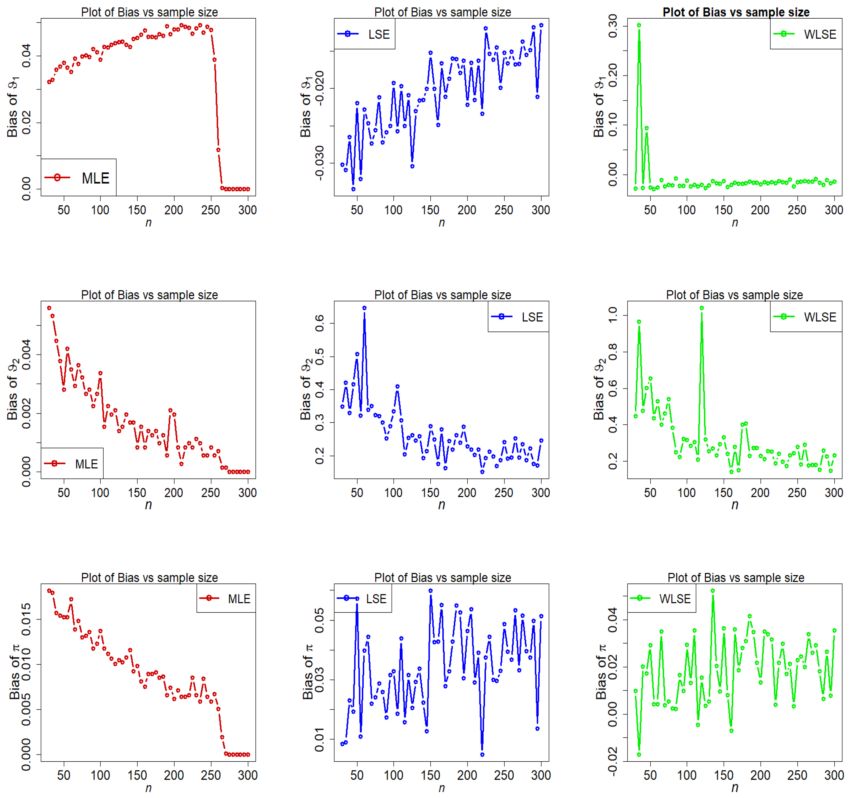
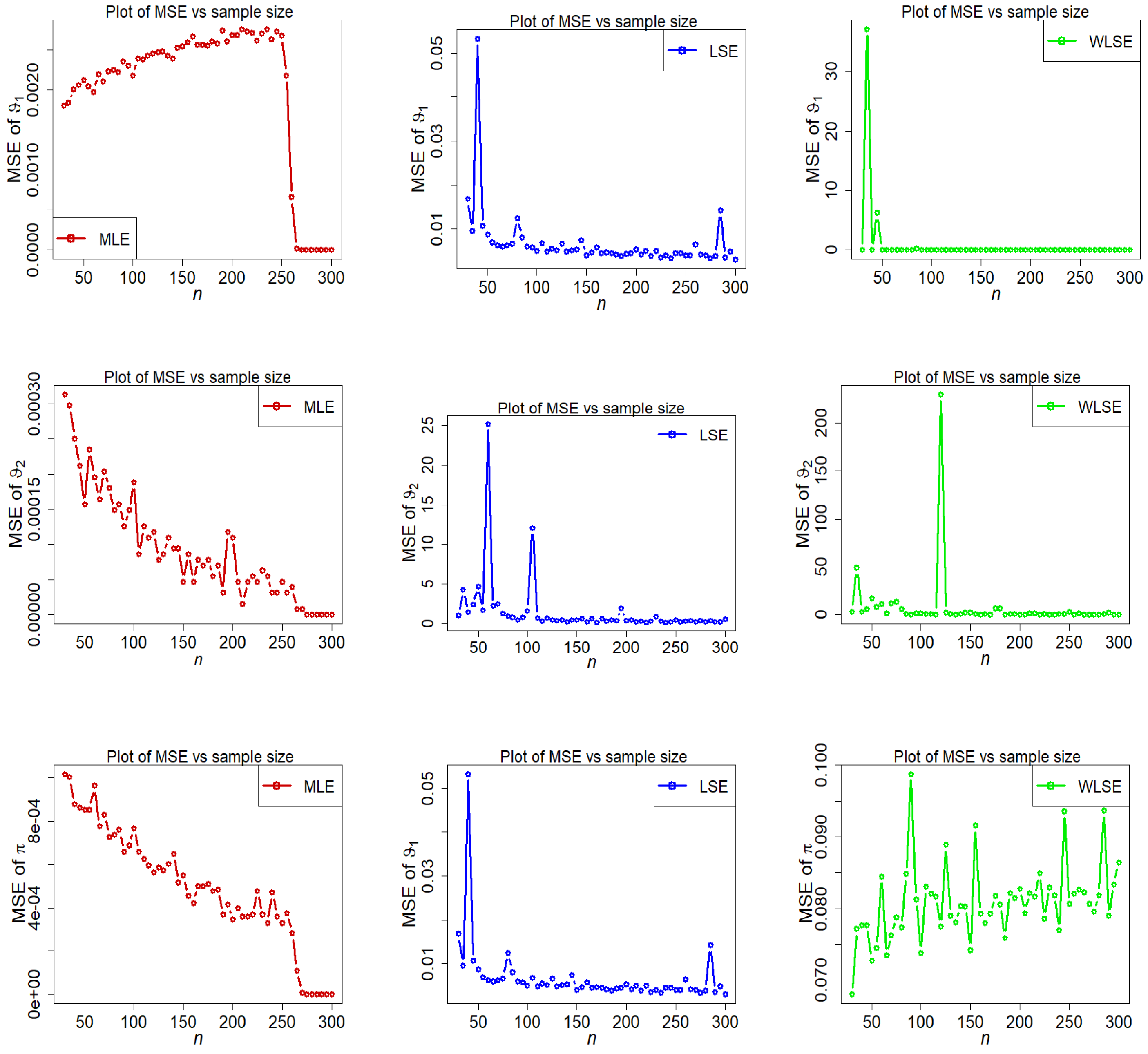
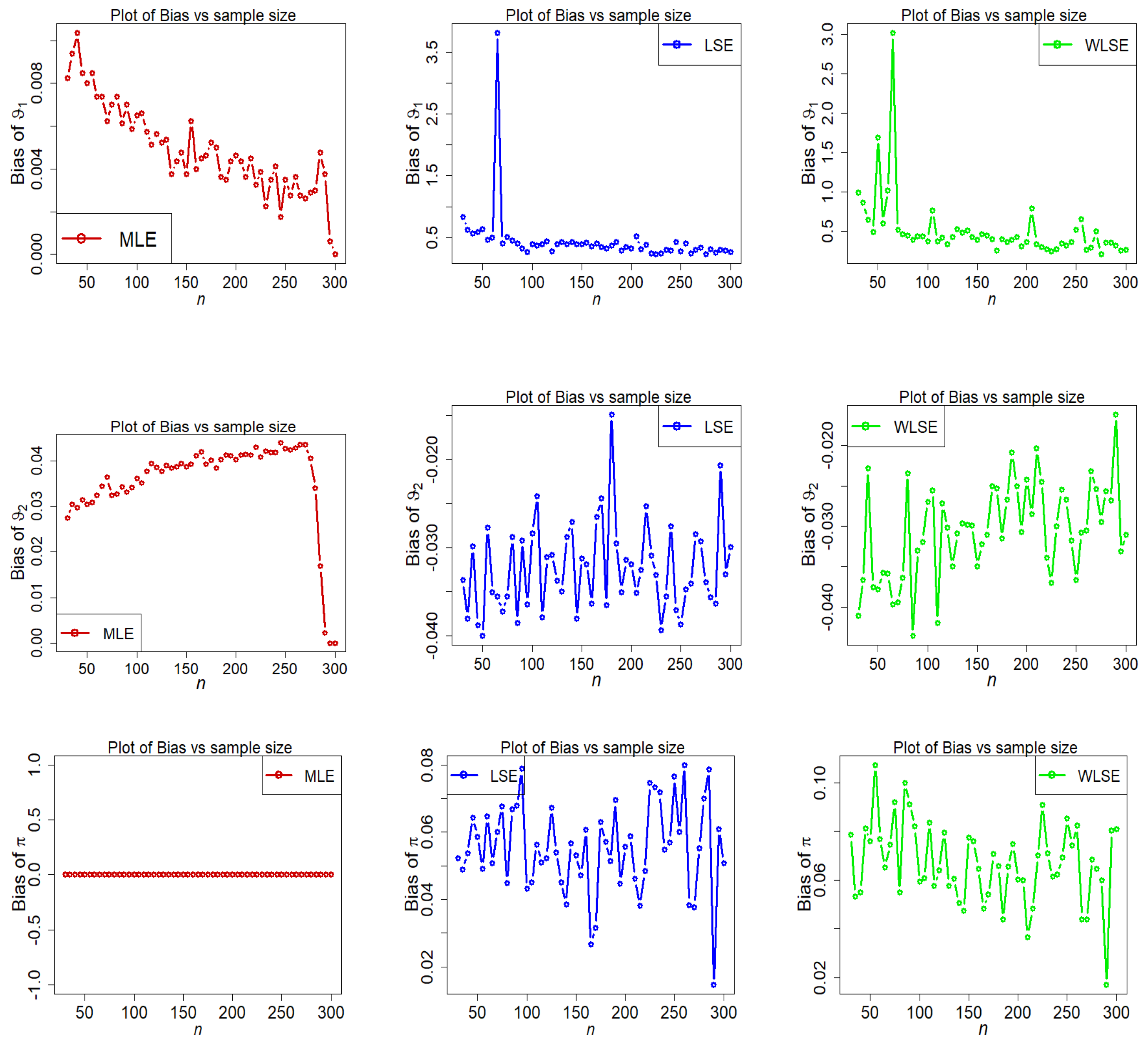
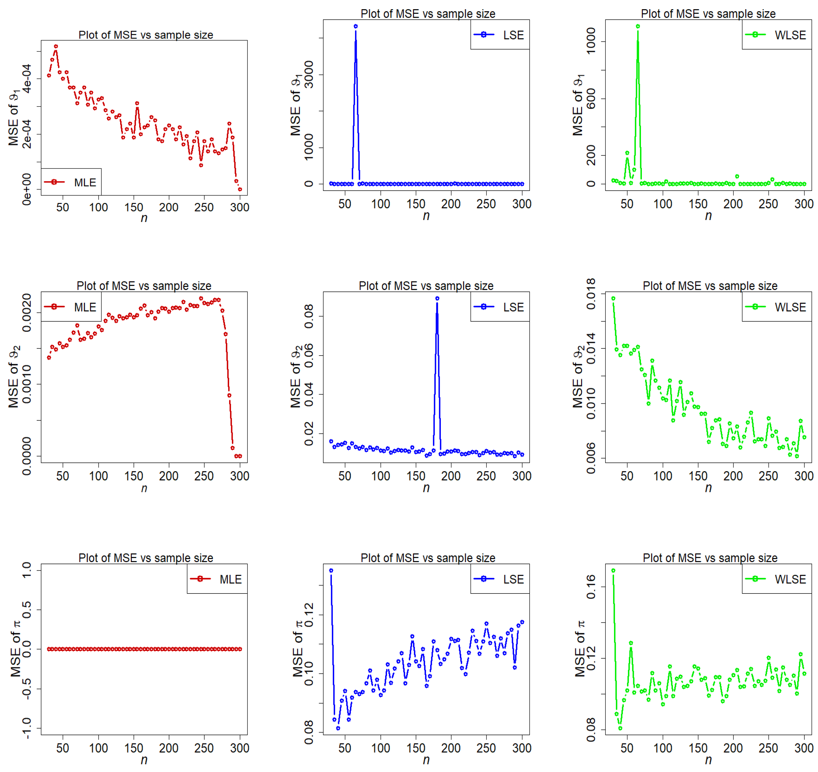
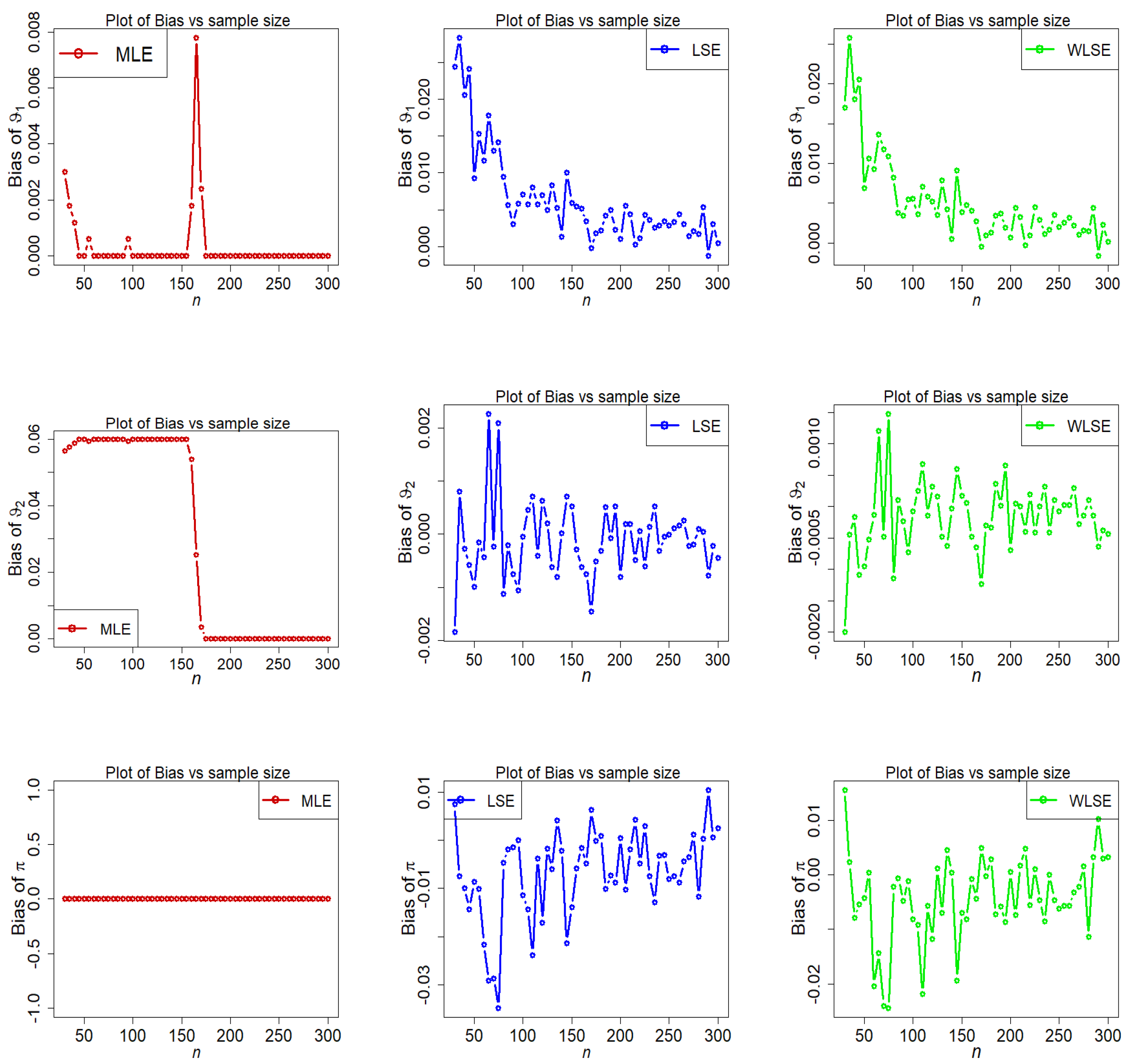
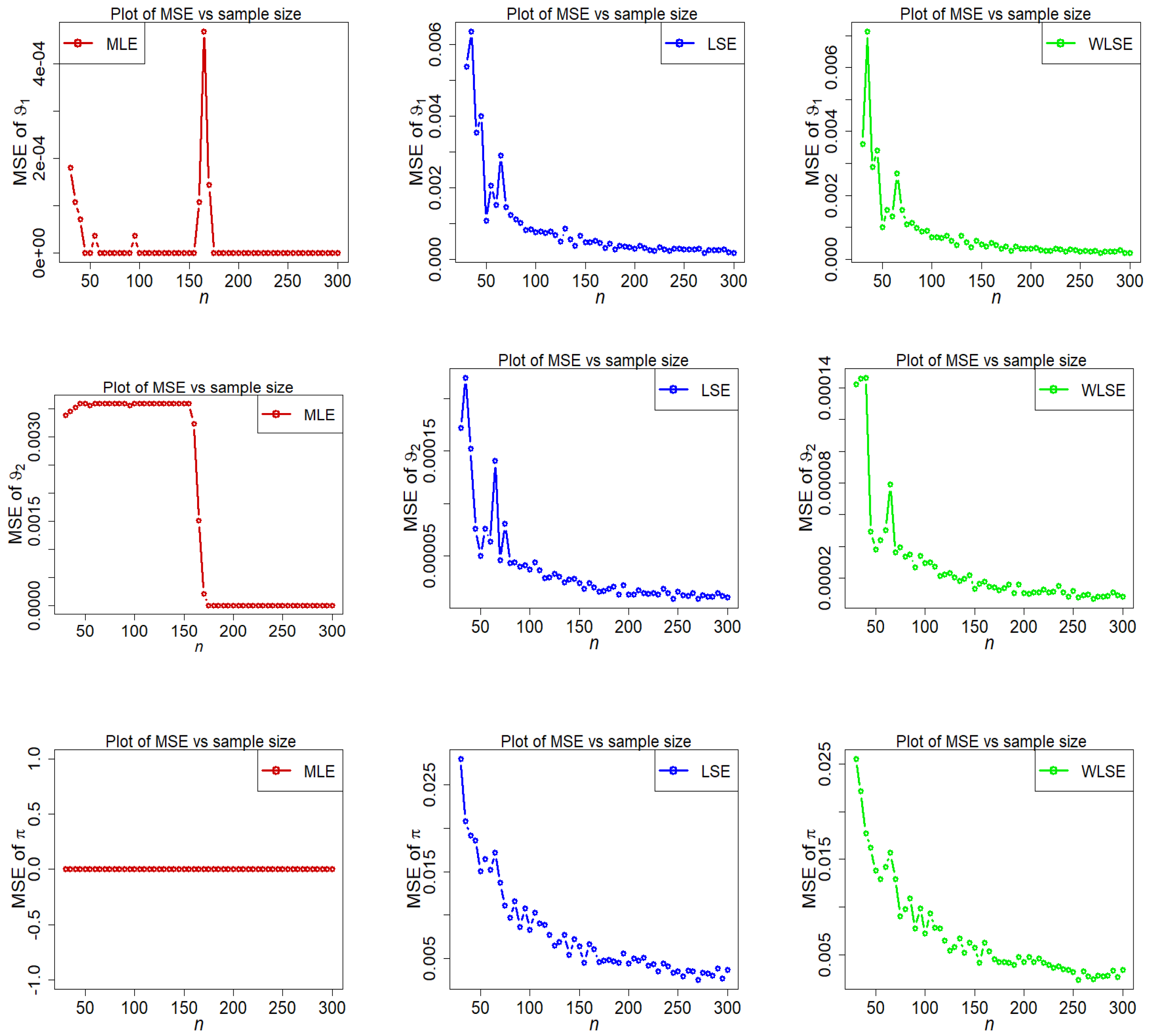
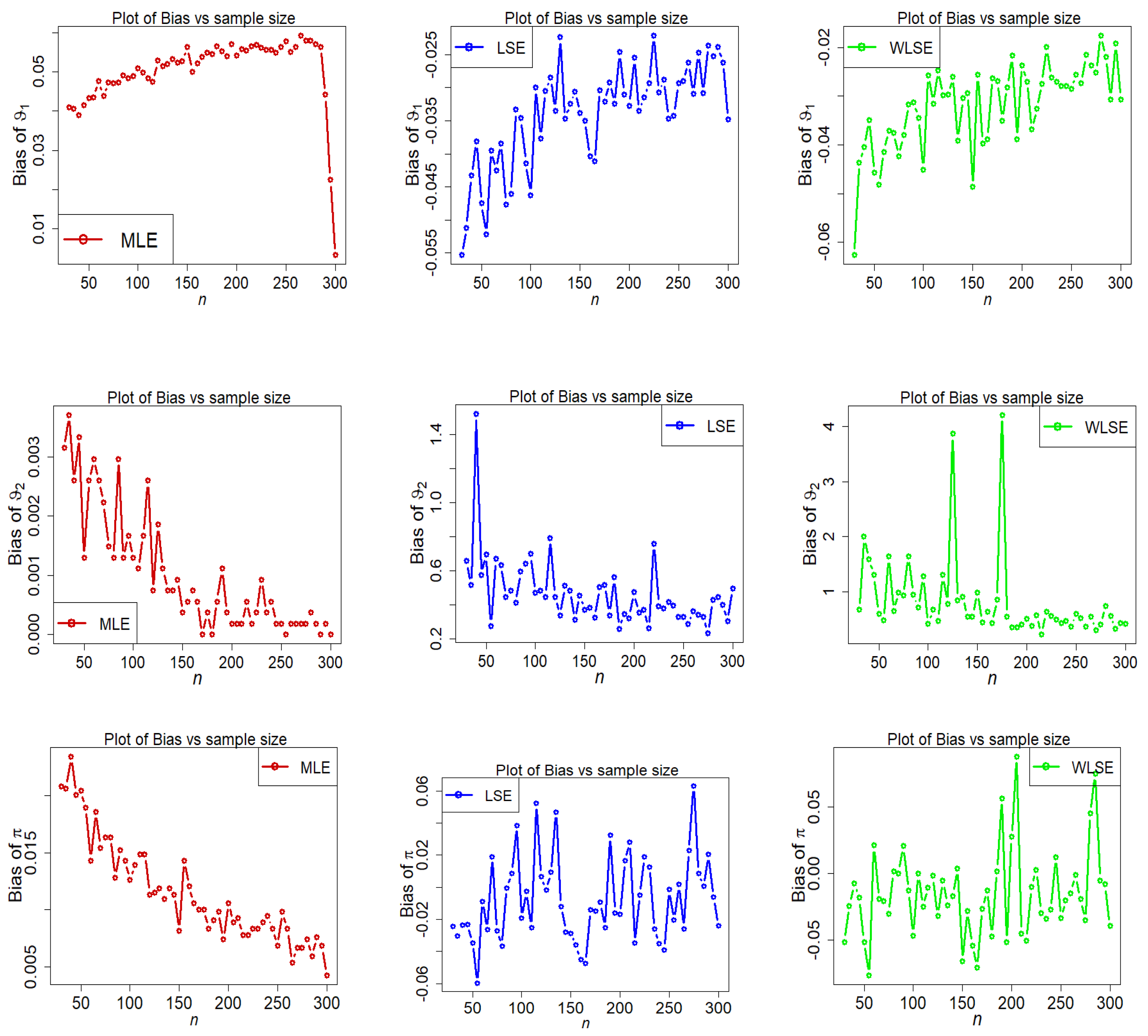
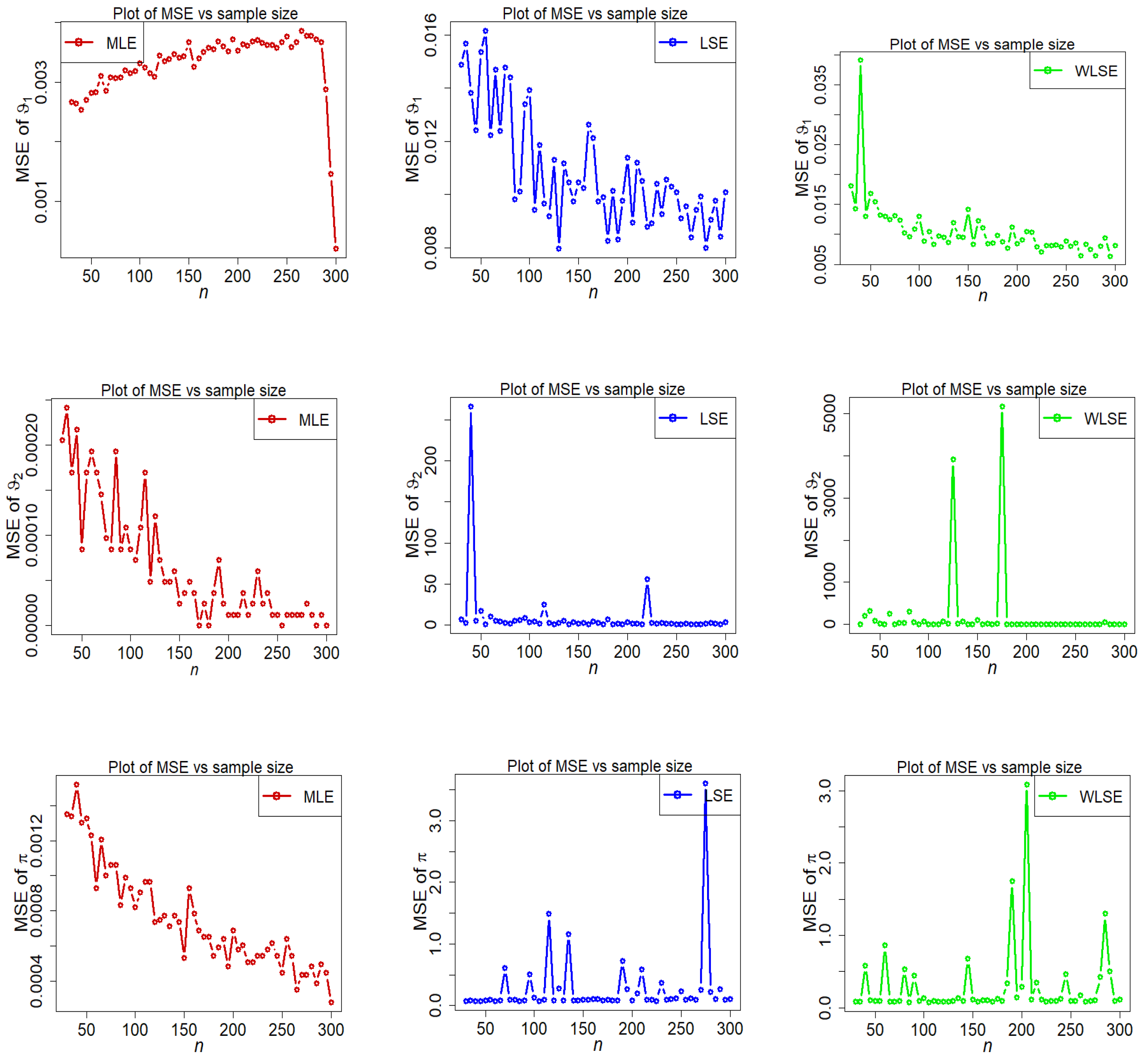
Figure 7, Figure 8, Figure 9, Figure 10, Figure 11, Figure 12, Figure 13 and Figure 14 display the empirical findings. These empirical results demonstrate that the 2-CMSM parameters may be accurately estimated using the suggested estimate methods. We can infer that the estimators display asymptotic unbiasedness because the bias goes to zero as n grows. On the other hand, the mean squared error behaviour suggests consistency because the mistakes trend to zero as n grows. The following observations can be drawn from Figure 7, Figure 8, Figure 9, Figure 10, Figure 11, Figure 12, Figure 13 and Figure 14.
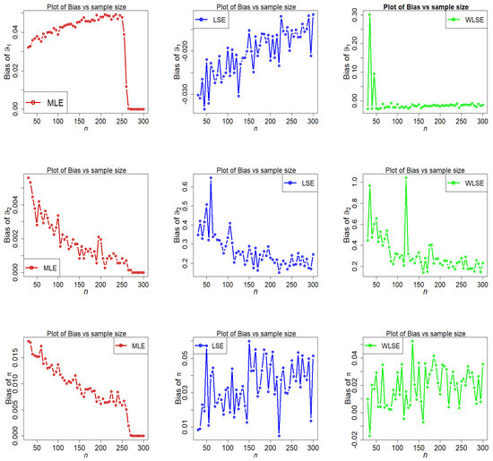
Figure 7.
Fluctuations of bias of estimators under different methods for parametric set I.
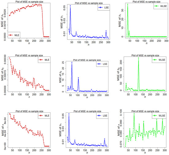
Figure 8.
Fluctuations of MSE of estimators under different methods for parametric set I.
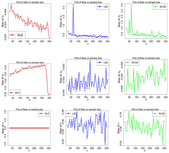
Figure 9.
Fluctuations of bias of estimators under different methods for parametric set II.
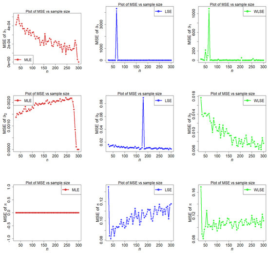
Figure 10.
Fluctuations of MSE of estimators under different methods for parametric set II.

Figure 11.
Fluctuations of bias of estimators under different methods for parametric set III.
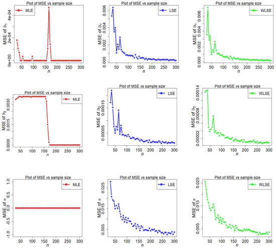
Figure 12.
Fluctuations of MSE of estimators under different methods for parametric set III.
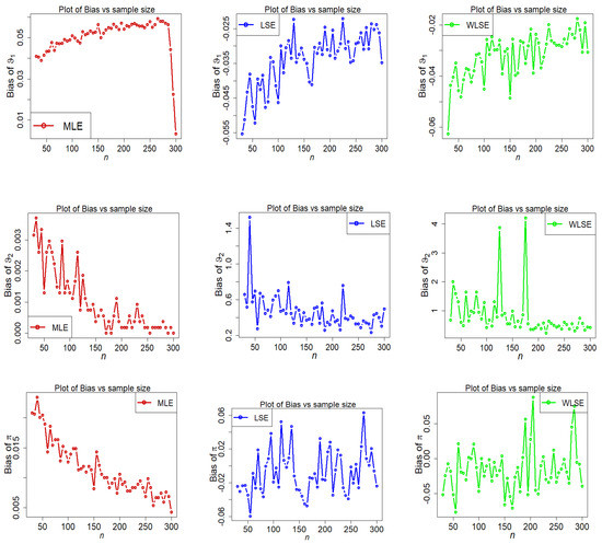
Figure 13.
Fluctuations of bias of estimators under different methods for parametric set IV.
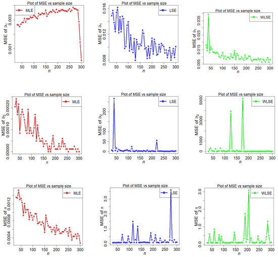
Figure 14.
Fluctuations of MSE of estimators under different methods for parametric set IV.
- The estimated bias of parameters , decreases as n increases under all three estimation approaches.
- For parametric Set-II, we can see that the estimated bias of parameters and is over-estimated in all three estimation methods, while is under-estimated in the LSE and WLSE estimation method (see Figure 9).
- The MSE of is strongly stimulated and higher under the LSE and WLSE estimation methods when (see Figure 10).
- Some big shifts in MSEs of under LSE and WLSE are observed when and .
- The discrepancy between estimates and assumed parameters goes to zero as the sample size grows in all estimating approaches.
The final finding from the above figures is that as the sample size grows, under all estimation methods, the estimated bias and MSE graphs for parameters , , and finally approach zero. This confirms the reliability of these estimating methods as well as the numerical computations for the 2-CMSM() parameters.
7. Applications
We demonstrate the flexibility of the 2-CMSM model in this section by examining two real-world datasets. The fits of the 2-CMSM model are compared to the competitive models such as the two component mixture of exponential model (2-CMEM and the two component mixture of Lindley (2-CMLM using the function maxLik() in R. The following excellently statistical benchmarks have been used to compare these models: -Log-likelihood (-LL), the AIC (Akaike information criterion), the BIC (Bayesian information criterion), and the AICC (Akaike information criterion corrected). The best model for the real data set might be the one with the lowest values of the above-mentioned goodness-of-fit (GOF) measures.
DataSet-1: Ghitany et al. [33] evaluated and analyzed the first data set, which represents the waiting times (in minutes) before the service of 100 Bank clients, in order to fit the Lindley distribution.
DataSet-2: The first set of data is from [34]; it is also analyzed by [35]. It comprises 40 measurements of active repair times for airborne communication transceivers. The hour is the unit of measurement.
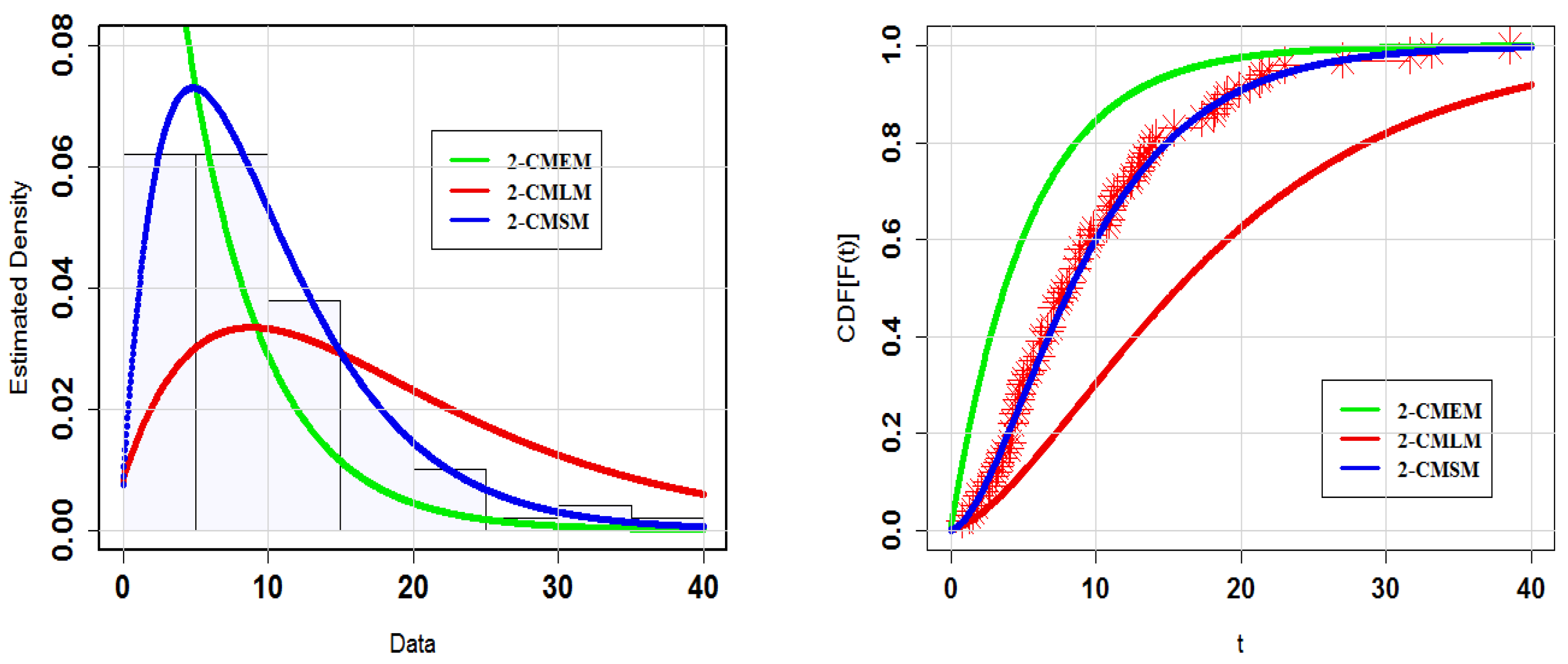
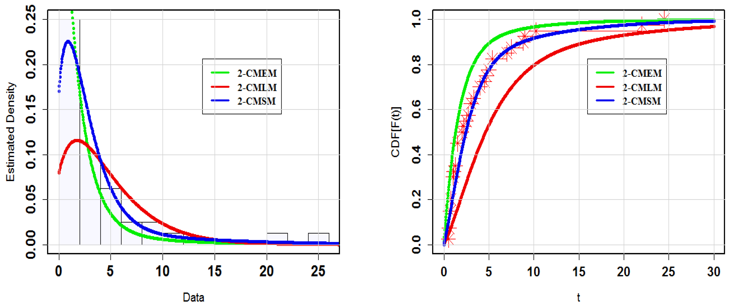
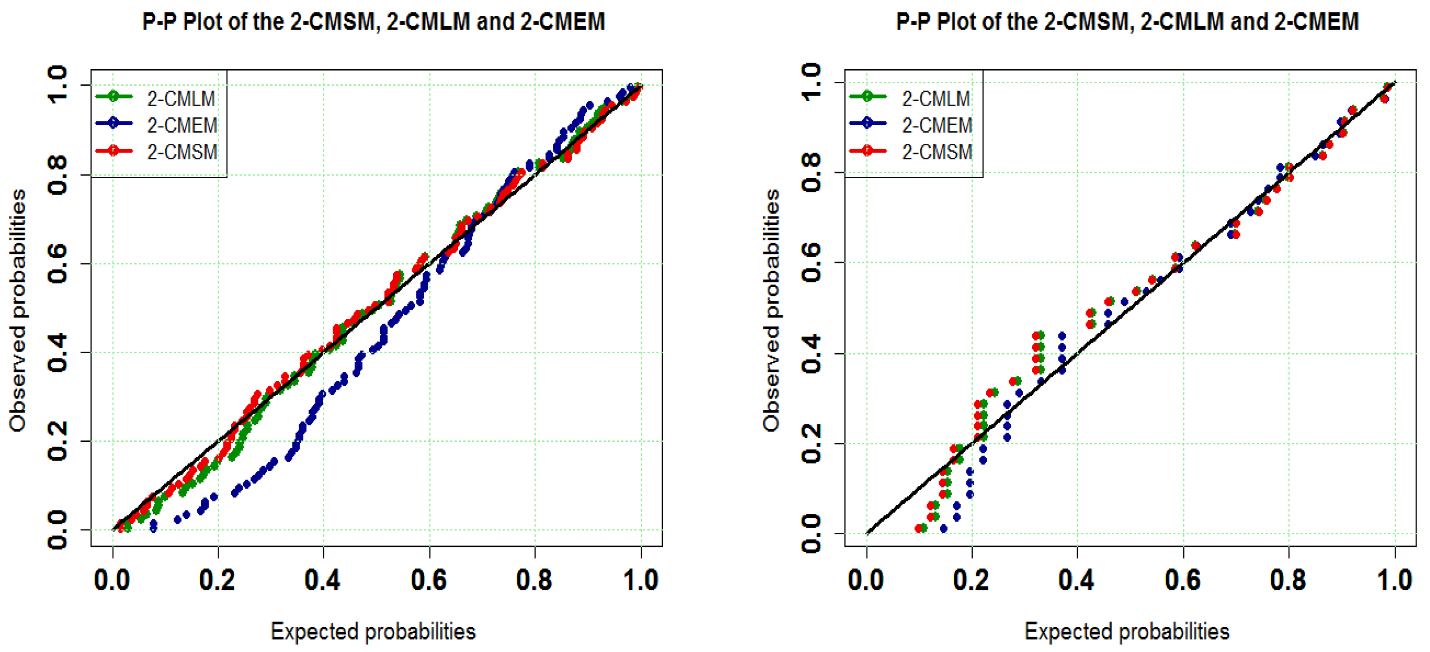
Table 1 and Table 2 show the MLEs for the 2-CMSM() and goodness-of-fit (GoF) metrics. Table 1 clearly demonstrates that the 2-CMSM() is superior to the 2-CMEM() and 2-CMLM(). For further visual detailed comparison of the estimated densities, the estimated PDFs and CDFs for the considered models for Datasets I and II have been graphed (Figure 15 and Figure 16). The CDF of the 2-CMSM(), yet again, is clearly closer to the empirical distribution than the 2-CMEM () and 2-CMLM(). To provide a different perspective, we employ probability–probability (PP) graphs in Figure 17 for Datasets I and II, respectively, to demonstrate the models’ adequacy. As seen in the Figures, the 2-CMSM() gives a very strong fit for these datasets when compared to 2-CMEM() and 2-CMLM(). Specifically, for Dataset II, it is obvious that the 2-CMSM() model provides a superior fit than the other models due to the exact adjustment of the scatter plot by the PP line. In summary, the 2-CMSM() model emerges as the more appropriate model for the two datasets, demonstrating its applicability in a real life situation.

Table 1.
MLEs, and GOF statistics for Dataset I.

Table 2.
MLEs, and GOF statistics for Dataset II.
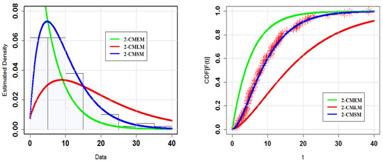
Figure 15.
Plots for the estimated PDFs and CDFs for Dataset I.
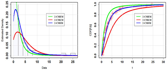
Figure 16.
Plots for the estimated PDFs and CDFs for Dataset II.
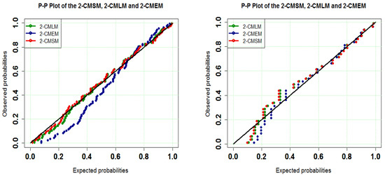
Figure 17.
The probability–probability (P-P) plots for Dataset I and II.
Figure 18 and Figure 19 show the profiles of the log-likelihood function (PLLF) based on datasets that support the findings of Table 1 and Table 2. Based on such graphical methods, we can suggest that the 2-CMSM () model is a better model for the data sets under consideration. Figure 18 and Figure 19 illustrate a graphical representation of the existence and uniqueness of MLEs, respectively.

Figure 18.
The PLLF for for Dataset I.

Figure 19.
The PLLF for Dataset II.
8. Conclusions
In this paper, we worked on two component mixtures of Shanker models using three estimate techniques: MLE, LSE, and WLSE. Additionally, the Shanker mixture model’s additional statistical and reliability characteristics, including central moments, cumulants, the cumulant generating function, the factorial-moment-generating function, the probability-generating function, skewness and kurtosis, the coefficient of variation, the Mills ratio, the mean time to failure, the reversed-hazard-rate function, and the mean residual life were obtained. To investigate and compare the performance of the estimation methodologies, a simulation study with 1000 iterations was carried out. As a consequence, we discovered that the ML technique performed better than the others in terms of accuracy and consistency while predicting model unknown parameters. Furthermore, we used real datasets to demonstrate the utility of the underlying mixture model. The current study can be expanded in the future by using a mixture model with more than two components.
Author Contributions
Conceptualization, T.N.S. and T.A.A.; Methodology, S.A.L., T.N.S. and M.K.H.H.; Software, T.A.A., A.S., T.N.S.; Validation, M.K.H.H., T.N.S.; Formal analysis, A.S., S.A.L., M.K.H.H. and T.A.A.; Investigation, A.S., S.A.L. and T.N.S.; Data curation, A.S., T.N.S.; Writing—original draft, A.S., T.N.S., M.K.H.H. and T.A.A.; Writing—review & editing, A.S. and T.A.A.; Supervision, A.S.; Funding acquisition, T.A.A. All authors have read and agreed to the published version of the manuscript.
Funding
The authors would like to thank the Deanship of Scientific Research at Umm Al-Qura University for supporting this work by Grant Code 22UQU4310063DSR13.
Data Availability Statement
The data used to support the findings of this study are included within the article.
Conflicts of Interest
The authors declare that have no conflict of interest.
Nomenclature
| Symbols | |
| RF | |
| CHRF | |
| Mills ratio | |
| MGF | |
| PGF | |
| CGF | |
| MTTF | |
| CDF | |
| HRF | |
| QF | |
| RF | |
| CF | |
| FMGF | |
| RHRF | |
| MRL |
Abbreviations
The following abbreviations are used in this manuscript:
| Probability density function | |
| PGF | Probability-generating function |
| CDF | Cumulative distribution function |
| FMGF | Factorial-moment-generating function |
| MLE | Maximum likelihood estimator |
| MGF | Moment-generating function |
| RHRF | Reversed-hazard-rate function |
| WLSE | Weighted least square estimator |
| CGF | Cumulant generating function |
| CHRF | Cumulative-hazard-rate function |
| TTF | Time-to-failure |
| QF | Quantile function |
| MTTF | Mean time to failure |
| HRF | Hazard rate function |
| MSE | Mean square error |
| CF | Characteristic function |
| RF | Reliability function |
| MRL | Mean residual life |
| MGF | Moment-generating function |
| LSE | Least square estimator |
References
- Everitt, B.S. A finite mixture model for the clustering of mixed-mode data. Stat. Probab. Lett. 1988, 6, 305–309. [Google Scholar] [CrossRef]
- Lindsay, B.G. Mixture models: Theory, geometry and applications. In NSF-CBMS Regional Conference Series in Probability and Statistics; Institute of Mathematical Statistics and the American Statistical Association: Beachwood, OH, USA, 1995; pp. 1–163. [Google Scholar]
- McLachlan, G.J.; Basford, K.E. Mixture Models: Inference and Applications to Clustering; M. Dekker: New York, NY, USA, 1988; Volume 38. [Google Scholar]
- McLachlan, G.; Peel, D. Finite Mixture Models; John Wiley & Sons: New York, NY, USA, 2000. [Google Scholar]
- Shi, J.Q.; Murray-Smith, R.; Titterington, D.M. Bayesian regression and classification using mixtures of Gaussian processes. Int. J. Adapt. Control. Signal Process. 2003, 17, 149–161. [Google Scholar] [CrossRef]
- Mohammad, D.; Muhammad, A. On the Mixture of BurrXII and Weibull Distribution. J. Stat. Appl. Probab. 2014, 3, 251–267. [Google Scholar]
- Sultan, K.S.; Ismail, M.A.; Al-Moisheer, A.S. Mixture of two inverse Weibull distributions: Properties and estimation. Comput. Stat. Data Anal. 2007, 51, 5377–5387. [Google Scholar] [CrossRef]
- Jiang, R.; Murthy, D.N.P.; Ji, P. Models involving two inverse Weibull distributions. Reliab. Eng. Syst. Saf. 2001, 73, 73–81. [Google Scholar]
- Mohamed, M.M.; Saleh, E.; Helmy, S.M. Bayesian prediction under a finite mixture of generalized exponential lifetime model. Pak. J. Stat. Oper. Res. 2014, 10, 417–433. [Google Scholar] [CrossRef]
- Mohammadi, A.; Salehi-Rad, M.R.; Wit, E.C. Using mixture of Gamma distributions for Bayesian analysis in an M/G/1 queue with optional second service. Comput. Stat. 2013, 28, 683–700. [Google Scholar] [CrossRef]
- Ateya, S.F. Maximum likelihood estimation under a finite mixture of generalized exponential distributions based on censored data. Stat. Pap. 2014, 55, 311–325. [Google Scholar]
- Sindhu, T.N.; Aslam, M. Preference of prior for Bayesian analysis of the mixed Burr type X distribution under type I censored samples. Pak. J. Stat. Oper. Res. 2014, 10, 17–39. [Google Scholar] [CrossRef]
- Al-Moisheer, A.S.; Daghestani, A.F.; Sultan, K.S. Mixture of Two One-Parameter Lindley Distributions: Properties and Estimation. J. Stat. Theory Pract. 2021, 15, 1–21. [Google Scholar] [CrossRef]
- Sindhu, T.N.; Riaz, M.; Aslam, M.; Ahmed, Z. Bayes estimation of Gumbel mixture models with industrial applications. Trans. Inst. Meas. Control 2016, 38, 201–214. [Google Scholar] [CrossRef]
- Sindhu, T.N.; Aslam, M.; Hussain, Z. A simulation study of parameters for the censored shifted Gompertz mixture distribution: A Bayesian approach. J. Stat. Manag. Syst. 2016, 19, 423–450. [Google Scholar] [CrossRef]
- Sindhu, T.N.; Feroze, N.; Aslam, M.; Shafiq, A. Bayesian inference of mixture of two Rayleigh distributions: A new look. Punjab Univ. J. Math. 2020, 48. [Google Scholar]
- Sindhu, T.N.; Khan, H.M.; Hussain, Z.; Al-Zahrani, B. Bayesian inference from the mixture of half-normal distributions under censoring. J. Natl. Sci. Found. Sri Lanka 2018, 46, 587–600. [Google Scholar] [CrossRef]
- Sindhu, T.N.; Hussain, Z.; Aslam, M. Parameter and reliability estimation of inverted Maxwell mixture model. J. Stat. Manag. Syst. 2019, 22, 459–493. [Google Scholar] [CrossRef]
- Ali, S. Mixture of the inverse Rayleigh distribution: Properties and estimation in a Bayesian framework. Appl. Math. 2015, 39, 515–530. [Google Scholar] [CrossRef]
- Zhang, H.; Huang, Y. Finite mixture models and their applications: A review. Austin Biom. Biostat. 2015, 2, 1–6. [Google Scholar]
- Shanker, R. Shanker Distribution and Its Applications. Int. J. Stat. Appl. 2015, 5, 338–348. [Google Scholar] [CrossRef]
- Shanker, R.; Fesshaye, H. On discrete Poisson-Shanker distribution and its applications. Biom. Biostat. Int. J. 2017, 5, 00121. [Google Scholar] [CrossRef]
- Shanker, R.; Hagos, F.; Sujatha, S. On modeling of lifetime data using one parameter Akash, Lindley and exponential distributions. Biom. Biostat. Int. J. 2016, 3, 1–10. [Google Scholar] [CrossRef]
- Shanker, R.; Hagos, F.; Sujatha, S. On modeling of Lifetimes data using exponential and Lindley distributions. Biom. Biostat. Int. J. 2015, 2, 1–9. [Google Scholar] [CrossRef]
- Dey, S.; Kumar, D.; Ramos, P.L.; Louzada, F. Exponentiated Chen distribution: Properties and estimation. Commun. Stat. Simul. Comput. 2017, 46, 8118–8139. [Google Scholar] [CrossRef]
- Dey, S.; Alzaatreh, A.; Zhang, C.; Kumar, D. A new extension of generalized exponential distribution with application to ozone data. Ozone Sci. Eng. 2017, 39, 273–285. [Google Scholar] [CrossRef]
- Rodrigues, G.C.; Louzada, F.; Ramos, P.L. Poisson exponential distribution: Different methods of estimation. J. Appl. Stat. 2018, 45, 128–144. [Google Scholar] [CrossRef]
- Dey, S.; Moala, F.A.; Kumar, D. Statistical properties and different methods of estimation of Gompertz distribution with application. J. Stat. Manag. Syst. 2018, 21, 839–876. [Google Scholar] [CrossRef]
- Dey, S.; Josmar, M.J.; Nadarajah, S. Kumaraswamy distribution: Different methods of estimation. Comput. Appl. Math. 2017, 37, 2094–2111. [Google Scholar] [CrossRef]
- Shafiq, A.; Sindhu, T.N.; Dey, S.; Lone, S.A.; Abushal, T.A. Statistical Features and Estimation Methods for Half-Logistic Unit-Gompertz Type-I Model. Mathematics 2023, 11, 1007. [Google Scholar] [CrossRef]
- Swain, J.J.; Venkatraman, S.; Wilson, J.R. Least-squares estimation of distribution functions in Johnson’s translation system. J. Stat. Comput. Simul. 1988, 29, 271–297. [Google Scholar] [CrossRef]
- Gupta, R.D.; Kundu, D. Generalized exponential distribution: Different method of estimations. J. Stat. Simul. 2001, 69, 315–337. [Google Scholar] [CrossRef]
- Ghitany, M.E.; Atieh, B.; Nadarajah, S. Lindley distribution and its application. Math. Comput. Simul. 2008, 78, 493–506. [Google Scholar] [CrossRef]
- Jorgensen, B. Statistical Properties of the Generalized Inverse Gaussian Distribution; Springer: New York, NY, USA, 1982. [Google Scholar]
- Bantan, R.A.; Jamal, F.; Chesneau, C.; Elgarhy, M. A New Power Topp–Leone Generated Family of Distributions with Applications. Entropy 2019, 21, 1177. [Google Scholar] [CrossRef]
Disclaimer/Publisher’s Note: The statements, opinions and data contained in all publications are solely those of the individual author(s) and contributor(s) and not of MDPI and/or the editor(s). MDPI and/or the editor(s) disclaim responsibility for any injury to people or property resulting from any ideas, methods, instructions or products referred to in the content. |
© 2023 by the authors. Licensee MDPI, Basel, Switzerland. This article is an open access article distributed under the terms and conditions of the Creative Commons Attribution (CC BY) license (https://creativecommons.org/licenses/by/4.0/).

