Longitudinal Data Analysis Based on Bayesian Semiparametric Method

Abstract

A Bayesian semiparametric model framework is proposed to analyze multivariate longitudinal data. The new framework leads to simple explicit posterior distributions of model parameters. It results in easy implementation of the MCMC algorithm for estimation of model parameters and demonstrates fast convergence. The proposed model framework associated with the MCMC algorithm is validated by four covariance structures and a real-life dataset. A simple Monte Carlo study of the model under four covariance structures and an analysis of the real dataset show that the new model framework and its associated Bayesian posterior inferential method through the MCMC algorithm perform fairly well in the sense of easy implementation, fast convergence, and smaller root mean square errors compared with the same model without the specified autoregression structure.

1. Introduction

Longitudinal data arise from repeated observations from the same individual or group of individuals at different time points. The structure of longitudinal data is shown in the following Table 1. The basic tasks of analyzing longitudinal data can be summarized as (1) studying the trend in the covariance structure of the observed variables with respect to time; (2) discovering the influence of covariates on the observable variables; and (3) determining the within-group correlation structures [1].

Table 1. Longitudinal data structures.

Observation Object	Number of Observations
	1	⋯	$k$
1	$t_{11},x_{1,11},\dots ,x_{p,11},y_{11}$	⋯	$t_{1k},x_{1,1k},\dots ,x_{p,1k},y_{1k}$
⋮	⋮		⋮
i	$t_{i1},x_{1,i1},\dots ,x_{p,i1},y_{i1}$	…	$t_{ik},x_{1,ik},\dots ,x_{p,ik},y_{ik}$
⋮	⋮		⋮
n	$t_{n1},x_{1,n1},\dots ,x_{p,n1},y_{n1}$	…	$t_{nk},x_{1,nk},\dots ,x_{p,nk},y_{nk}$

Note: In Table 1, $t_{ij}$ stands for the j-th observation time of the individual i; $(x_{1,ij},\dots ,x_{p,ij})$ for the p-dimensional covariate of individual i at $t_{ij}$; and $y_{ij}$ for the j-th observation of individual i.

Longitudinal data are often highly unbalanced. It is usually difficult to apply traditional multiple regression techniques to analyze highly unbalanced data directly. Statisticians developed various Bayesian statistical inference models for longitudinal data analysis [2]. A parametric assumption may result in modeling bias and may relax the assumption about parametric structure. Nonparametric methods have the characteristics of robustness because they do not require model assumptions. Semiparametric models integrate the characteristics of parametric and nonparametric models and have the characteristics of flexibility and ease of interpretation. Nonparametric statistical methods and semiparametric statistical methods are not only hot spots in current statistical research but also widely used in many practical applications. Xiang et al. [3] summarize some common outcomes of nonparametric regression analysis of longitudinal data. Bayesian methods for parametric linear mixed models have been widely used in different areas. Assuming a normal random effect and using the standard Gibbs sampling to realize some simple posterior inference, Quintana et al. [4] extend the general class of mixed models for longitudinal data by generalizing the GP part to the nonparametric case. The GP is a probabilistic approach to learning nonparametric models. Cheng et al. [5] propose the so-called LonGP, which is a flexible and interpretable nonparametric modeling framework. It provides a versatile software implementation that can solve commonly faced challenges in longitudinal data analysis. It also develops a fully Bayesian, predictive inference for LonGP, which can be employed to carry out model selection. Kleinman and Ibrahim [6] relax the normal assumption by assuming a Dirichlet process prior with a Gaussian measure of zero mean, semiparametrically modeling the random effects distribution [7]. Although a parametric model may have limitations in some applications, it is simpler than a nonparametric model whose scope may be too wide to draw a concise conclusion. Nonparametric regression has a fatal weakness, known as the “curse of dimensionality”, which refers to the fact that when the independent variable X is multivariate, the estimation accuracy of the regression function becomes very poor as the dimension of X increases. To solve this problem, the semiparametric model is a good compromise maintaining some excellent characteristics of parametric and nonparametric models [8]. There is a lot of literature on the semiparametric modeling of longitudinal data. Most of the existing literature employs random effects to model within-group correlations [9].

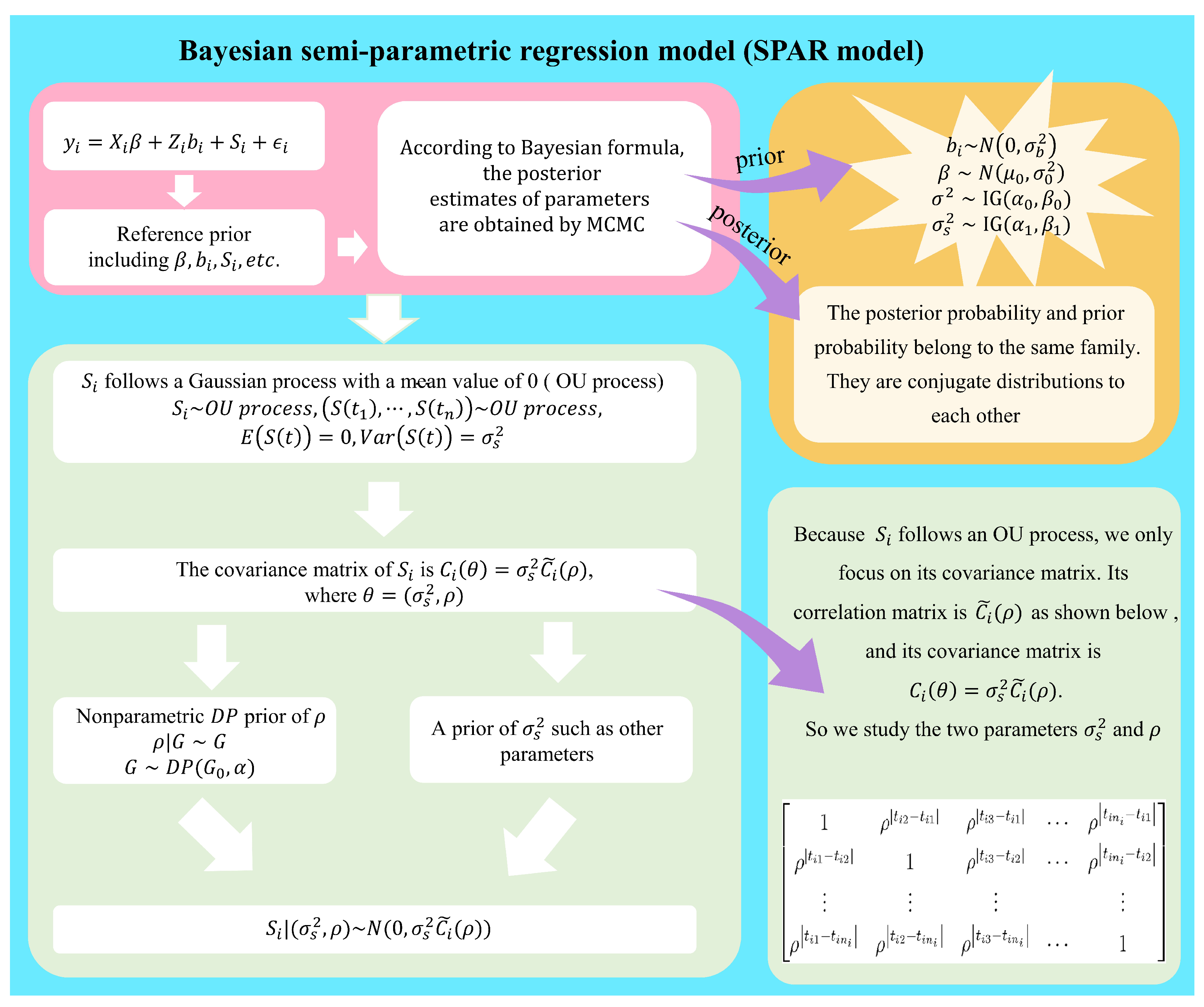
Semiparametric linear mixed models generalize traditional linear mixed models by modeling a covariate effect with a nonparametric function and parametrically modeling other covariate effects. Semiparametric linear mixed models mainly use frequentist methods for statistical inference and assume normal random effects [10]. In this paper, we employ a Bayesian semiparametric framework for linear mixed models given by Quintana et al. [4] by imposing stronger conditions on the random effect to obtain an explicit solution to posterior distributions of the model parameters and fast convergence of the MCMC algorithm in the posterior inference of model parameters. The proposed framework generalizes the default priori of variance components and adjusts the inference of fixed effects associated with nonparametric random effects. The latter includes the extrapolation of nonparametric mean functions over time [11,12]. The stochastic process approach in [4] is a good choice for characterizing the intragroup correlation. The Gaussian process (GP) covariance has an exponential form and is uniquely determined by two parameters. GP can specify autoregressive correlation (the AR covariance structure, [13]). A nonparametric Dirichlet process (DP) priori assigned to the covariance parameter results in an Ornstein–Uhlenbeck process (OUP). A partial Dirichlet process mixture (DPM) is performed on the OUP. By imposing stronger conditions on the random effect and decomposing the OUP into some single Gaussian variables, we can substantially simplify the MCMC sampling in the posterior inference. The framework of our proposed semiparametric autoregression model (SPAR) is demonstrated in Figure 1.

Figure 1. Bayesian semiparametric autoregression model (SPAR model).

This paper is organized as follows. Section 2 briefly introduces some basic theoretical background and principles. Section 3 introduces the model setup using a partial Dirichlet process mixture in terms of the OUP, and the Bayesian semiparametric autoregressive model is proposed with a recommended solution. In Section 4, the Dirichlet process and Dirichlet process mixture (DPM) are simply introduced. The formulation of the semiparametric autoregressive model is given in Section 5. Section 6 derives the marginal likelihood, prior determination, and posteriori inference. Section 7 gives a simple Monte Carlo study and a real dataset application based on the proposed model. Some concluding remarks are given in the last section.

2. Theoretical Basis

2.1. A General Linear Hybrid Model Containing an AR Structure

For an observation object $i(i=1,2,\dots ,n)$, we denote the observation time points by $\left\{t_{i1},t_{i2},\dots ,t_{i{n}_i}\right\}$. Let ${\mathit{y}}_i={(y_{i1},y_{i2},\dots ,y_{i{n}_i})}^{\prime }$ ($n_i\times 1$) be the observation vector from object i. At time point $t_{ij}$, we consider the possible time-dependent covariate vector ${\mathit{x}}_{ij}^{\prime }=(1,x_{i1}\left(t_{ij}\right),x_{i2}\left(t_{ij}\right),\dots ,x_{ip}\left(t_{ij}\right))$. Let ${\mathit{y}}_i={(y_{i1},y_{i2},\dots ,y_{i{n}_i})}^{\prime }$ ($n_i\times 1$) be the observation vector from object i. At time point $t_{ij}$, we consider the possible time-dependent covariate vector ${\mathit{x}}_{ij}^{\prime }=(1,x_{i1}\left(t_{ij}\right),x_{i2}\left(t_{ij}\right),\dots ,x_{ip}\left(t_{ij}\right))$. Let $E\left(y_{ij}\right)={\mathit{x}}_{ij}^{\prime }\mathit{\beta }$. Define the $n_i\times (p+1)$-dimensional fixed-effect design matrix ${\mathit{X}}_i={({\mathit{x}}_{i1},{\mathit{x}}_{i2},\dots ,{\mathit{x}}_{i{n}_i})}^{\prime }$. Assume $E\left({\mathit{y}}_i\right)={\mathit{X}}_i\mathit{\beta }$. Define the corresponding $n_i\times q(q\le p)$-dimensional random effects design matrix ${\mathit{Z}}_i={({\mathit{z}}_{i1},{\mathit{z}}_{i2},\dots ,{\mathit{z}}_{i{n}_i})}^{\prime }$, where ${\mathit{z}}_{ij}^{\prime }=(1,z_{i1}\left(t_{ij}\right),z_{i2}\left(t_{ij}\right),\dots ,z_{iq}\left(t_{ij}\right))$. The general linear mixed model containing an AR covariance structure is

$$\begin{array}{cc}\hfill {\mathit{y}}_i& ={\mathit{X}}_i\mathit{\beta }+{\mathit{Z}}_i{\mathit{b}}_i+{\mathit{S}}_i+{ϵ}_i,\hfill \\ \hfill {\mathit{b}}_i|\tau & \sim N(\mathit{0},\mathit{D}(\tau \left)\right),\hfill \end{array}\begin{array}{cc}\hfill {\mathit{S}}_i|\theta & \sim N(\mathit{0},{\mathit{C}}_i\left(\theta \right)),\hfill \\ \hfill {ϵ}_i& \sim N(\mathit{0},{\sigma }^2{\mathit{I}}_{n_i}),\hfill \end{array}$$

(1)

where ${\mathit{X}}_i\mathit{\beta }$ stands for the fixed effect and ${\mathit{Z}}_i{\mathit{b}}_i$ for the random effect, ${\mathit{S}}_i$ is a stochastic process characterizing the correlation among the $n_i$ observations from object i, ${ϵ}_i$ is the error term, $i=1,2,\dots ,n_i$. ${\mathit{C}}_i\left(\theta \right)$ is an $n_i\times n_i$ structural covariance matrix, and vectors $\tau$ and $\theta$ contain the variance–covariance parameters of the random vector ${\mathit{b}}_i$ and the stochastic process ${\mathit{S}}_i$, respectively. ${\mathit{I}}_{n_i}$ stands for the identity matrix of dimension $n_i\times n_i$. The AR structure is usually specified by a GP with zero mean. The GP is uniquely determined by a covariance function containing parameter $\theta =({\sigma }_s,\rho )$. The vector ${\mathit{S}}_i$ is a GP corresponding to the i-th object. ${\mathit{S}}_i$ is generated sequentially by the GP $\{s_i\left(t\right):t>0\}$ at the observation time points $\{t_{i1},t_{i2},\dots ,t_{i{n}_i}\}$, i.e.,

$${\mathit{S}}_i=\left(s_i\left(t_{i1}\right),s_i\left(t_{i2}\right),\dots ,s_i\left(t_{i{n}_i}\right)\right).$$

To specify the AR structure, it is assumed that the above GP possesses stationarity:

$$\mathrm{Cov}(s_i\left(t_{il}\right),s_i\left(t_{ik}\right))={\sigma }_s^2\rho \left(\right|t_{il}-t_{ik}\left|\right).$$

(2)

When the model has a structured covariance function, the covariance matrix of ${\mathit{y}}_i$ is

$$\mathrm{Cov}\left({\mathit{y}}_i\right)={\mathit{Z}}_i\mathit{D}\left(\tau \right){\mathit{Z}}_i^{\prime }+{\mathit{C}}_i\left(\theta \right)+{\sigma }^2{\mathit{I}}_{n_i}.$$

(3)

2.2. The Principle for Bayesian Inference

The Bayesian method assumes a piori distribution on the unknown parameter $\theta$ and a joint distribution $p(\mathit{x},\theta )$ between an observable variable X and the parameter $\theta$. The Bayesian method is based on the posterior distribution $\pi \left(\theta \right|\mathit{x})$ of the unknown parameter $\theta$ after observed data are available. The joint distribution, the priori distribution, and the posterior distribution are related to each other as follows:

$$\begin{array}{cc}\hfill p(\mathit{x},\theta )& =\pi \left(\theta \right|\mathit{x})p_{\mathit{X}}\left(\mathit{x}\right),\hfill \\ \hfill p_{\mathit{X}}\left(\mathit{x}\right)={\int }_{\mathsf{\Theta }}p(\mathit{x},\theta )& \mathrm{d}\theta ={\int }_{\mathsf{\Theta }}p\left(\mathit{x}\right|\theta )\pi \left(\theta \right)\mathrm{d}\theta ,\hfill \end{array}$$

where $p_{\mathit{X}}\left(\mathit{x}\right)$ stands for the sample marginal density of $\mathit{x}$. We use the posterior distribution $\pi \left(\theta \right|\mathit{x})$ to carry out statistical inference for the parameter $\theta$:

$$\pi \left(\theta \right|\mathit{x})=\frac{p(\mathit{x},\theta )}{p_{\mathit{X}}\left(\mathit{x}\right)}=\frac{p\left(\mathit{x}\right|\theta \left)\pi \right(\theta )}{{\int }_{\mathsf{\Theta }}p\left(\mathit{x}\right|\theta )\pi \left(\theta \right)\mathrm{d}\theta }$$

(4)

Equation (4) is the well-known Bayesian formula. Bayesian statistical inference assumes that the posterior distribution of the unknown parameter $\theta$, $\pi \left(\theta \right|\mathit{x})$ contains all the available information. As a result, the point estimation, interval estimation, hypothesis testing, and predicting inference of $\theta$ can be implemented as usual. Because

$$\pi \left(\theta \right|\mathit{x})=\frac{\pi \left(\theta \right)p\left(\mathit{x}\right|\theta )}{{\int }_{\mathsf{\Theta }}\pi \left(\theta \right)p\left(\mathit{x}\right|\theta )\mathrm{d}\theta }\propto \pi \left(\theta \right)p\left(\mathit{x}\right|\theta ),$$

we construct the Bayesian estimate for $\theta$ after observing data $\mathit{x}$ by their conditional expectation:

$$\widehat{\theta }=E\left(\theta \right|\mathit{x})=\frac{{\int }_{\mathsf{\Theta }}\pi \left(\theta \right)p\left(\mathit{x}\right|\theta )\theta \mathrm{d}\theta }{{\int }_{\mathsf{\Theta }}\pi \left(\theta \right)p\left(\mathit{x}\right|\theta )\mathrm{d}\theta }\propto {\int }_{\mathsf{\Theta }}\pi \left(\theta \right)p\left(\mathit{x}\right|\theta )\theta \mathrm{d}\theta .$$

(5)

In general, the Bayesian estimate $\widehat{g}\left(\theta \right)$ for a function of $\theta$, $g\left(\theta \right)$ can be obtained as follows:

$$\widehat{g}\left(\theta \right)=E\left[g\left(\theta \right)\right|\mathit{x}]=\frac{{\int }_{\mathsf{\Theta }}\pi \left(\theta \right)p\left(\mathit{x}\right|\theta )g\left(\theta \right)\mathrm{d}\theta }{{\int }_{\mathsf{\Theta }}\pi \left(\theta \right)p\left(\mathit{x}\right|\theta )\mathrm{d}\theta }\propto {\int }_{\mathsf{\Theta }}\pi \left(\theta \right)p\left(\mathit{x}\right|\theta )g\left(\theta \right)\mathrm{d}\theta .$$

Obviously, the estimator $\widehat{g}\left(\theta \right)$ is the usual expectation of $g\left(\theta \right)$ with respect to the posterior distribution $\pi \left(\theta \right|\mathit{x})$:

$$\widehat{g}\left(\theta \right)={\int }_{\mathsf{\Theta }}g\left(\theta \right)\pi \left(\theta \right|\mathit{x})\mathrm{d}\theta =E\left[g\left(\theta \right)|\mathit{x}\right].$$

(6)

2.3. The MCMC Sampling and Its Convergence

When the posterior distribution $\pi \left(\theta \right|\mathit{x})$ in (6) is difficult to compute, estimating multiple parameters given by $g\left(\theta \right)$ can be realized by the Markov Chain Monte Carlo (MCMC) method [14] following these steps: (1) establish a Markov chain, the stationary distribution for $\pi \left(\theta \right|\mathit{x})$; (2) use the Markov chain for the posterior distribution $\pi \left(\theta \right|\mathit{x})$ to carry out sampling to obtain an MCMC sample $\{{\theta }_0,{\theta }_1,\dots ,{\theta }_n\}$; and (3) obtain the MCMC estimator $\widehat{g}\left(\theta \right)$ for $g\left(\theta \right)$ by

$$\widehat{g}\left(\theta \right)=\overline{g}\left(\theta \right)=\frac{1}{n}\sum _{i=1}^{n}g\left({\theta }_i\right).$$

The MCMC sample can estimate the parameter function $g\left(\theta \right)$ more and more effectively when the sample size n becomes larger and larger. The MCMC sample $\{{\theta }_0,{\theta }_1,{\theta }_2,\dots ,\}$ possesses some properties, such as stability, normal recurrence, periodicity, and irreducibility. The choice of the initial value ${\theta }_0$ has little impact on the estimate of ${\theta }_t$. Gibbs sampling is one of the MCMC algorithms. It is used to construct a multivariate probability distribution of a random sample. The defect of the standard Gibbs sampling is that it cannot process the nonconjugated distribution. Because the prior distribution of parameter $\rho$ in the model in this paper is nonconjugated, the improved version of the Gibbs algorithm is adopted [15].

With regard to the convergence of the MCMC sampling, we consider three convergence criteria: (1) Combine the posterior sampling trend graph with the energy graph of the MCMC sampling process for convergence assessment. By observing the posterior sampling trend graph of a random variable, we can determine if the information of the sampling tends to be stable as the number of iterations increases. (2) Compare the overall distribution of energy levels in real data with energy changes between successive samples. If the two distributions are similar to each other, we can conclude that the algorithm converges. (3) Draw the trajectory of the negative evidence lower bound (ELBO, [16]) obtained in the optimization process to verify the convergence of the algorithm. Minimizing the KL (Kullback–Leibler) divergence is equivalent to minimizing the negative ELBO [17,18].

3. The OU Process

The random process $S_i$ in the general linear mixed model (1) is a Gaussian process (GP). A GP can be regarded as an infinite dimensional extension of the multivariate Gaussian distribution, and its probability characteristics are uniquely determined by the mean function and covariance function. In particular, a GP with zero mean is completely determined by its covariance function [18]. To give a simple review of GP and keep the notation $S_i$ specially used in model (1), we return to a general notation $X\left(t\right)$ for GP to avoid a mix-up with the model parameter in model (1). $X\left(t\right)$ in this section can be considered as a copy of $S_i$ in model (1). If random process $\left\{X\right(t),t\in \mathit{T}\}$ is a GP, any finite observation vector $x={\left(X\left(t_1\right),\dots ,X\left(t_n\right)\right)}^{\prime }$ has a multivariate Gaussian distribution. Let $E\left[X\left(t\right)\right]=m_X\left(t\right),var\left[X\left(t\right)\right]={\sigma }_X^2\left(t\right)$. The joint density function of the multivariate Gaussian random vector is

$$f\left(x\left(t_1\right),\dots x\left(t_n\right)\right)={\left(2\pi \right)}^{-\frac{n}{2}}{\left|{\mathit{C}}_X\right|}^{-\frac{1}{2}}exp\left\{-\frac{1}{2}{\left(\mathit{x}-{\mathit{m}}_X\right)}^{\prime }{\mathit{C}}_X^{-1}\left(\mathit{x}-{\mathit{m}}_X\right)\right\},$$

where $x={\left(x\left(t_1\right),\dots ,x\left(t_n\right)\right)}^{\prime }$, mean vector ${\mathit{m}}_X={\left(m_X\left(t_1\right),\dots ,m_X\left(t_n\right)\right)}^{\prime }$, and ${\mathit{C}}_X$ stands for the covariance matrix. Let $c_{ij}=\mathrm{cov}\left(X\left(t_i\right),X\left(t_j\right)\right)=E\left[(X\left(t_i\right)-m_X\left(t_i\right))(X\left(t_j\right)-m_X\left(t_j\right))\right]$. When the Gaussian process $\{X_t=X\left(t\right),t\in \mathit{T}\}$ has a zero mean and it is smooth, we have $c_{ij}=E\left[X\left(t_i\right)X\left(t_j\right)\right]$ and

$$\begin{array}{cc}\hfill E\left[X\right(t\left)\right]& =0\hfill \\ \hfill \mathrm{var}\left[X\right(t\left)\right]& ={\sigma }_X^2\hfill \\ \hfill R_X\left(X_t,X_s\right)& =E\left[\left(X_t\right)\left(X_s\right)\right]=R_X(t-s),t>s,\hfill \\ \hfill C_X\left(X_t,X_s\right)& ={\sigma }_X^2{R}_X(t-s)=C_X(t-s),t>s,\hfill \end{array}$$

where $R_X\left(X_t,X_s\right)$ and $C_X\left(X_t,X_s\right)$ stand for the GP autocorrelation function and the autocovariance function, respectively, which only depend on the time interval $t-s$. Thus, $R_X(t-s)=\rho \left(\right|t-s\left|\right)$, and $c_{ij}=\mathrm{cov}\left(X\left(t_i\right),X\left(t_j\right)\right)={\sigma }_X^2\rho \left(\right|t_i-t_j\left|\right)$. The correlation coefficient between $X\left(t_i\right)$ and $X\left(t_j\right)$ is denoted by $\rho \left(\right|t_i-t_j\left|\right)$. It is assumed that $\rho \left(\right|t_i-t_j\left|\right)={\rho }^{|t_i-t_j|}$ in this paper. A zero-mean smooth GP $\left\{X\right(t),t\in \mathit{T}\}$ is an Ornstein–Uhlenbeck (OU) process [19]. An OU process can be regarded as a continuous analogy of the discrete-time first-order autoregressive AR(1) process.

To understand some properties of the AR(1) process, we express the AR(1) process as

$$X_t={\varphi }_1{X}_{t-1}+{ϵ}_t,t\ge 1,X_0={ϵ}_0,$$

(7)

where $|{\varphi }_1|<1$ is a weight parameter to ensure stability, and ${ϵ}_0,{ϵ}_1,{ϵ}_2,\dots$ are uncorrelated random variables satisfying

$$E\left({ϵ}_t\right)=0,t\ge 0,Var\left({ϵ}_t\right)=\left\{\begin{array}{cc}\frac{{\sigma }^2}{1-{\varphi }_1^2},\hfill & t=0,\hfill \\ {\sigma }^2,\hfill & t\ge 1.\hfill \end{array}\right..$$

It is assumed that the random error satisfies $\mathrm{cov}({ϵ}_t,{ϵ}_{t+k})=0,k\ne 0$. Therefore,

$$\begin{array}{cc}& {\displaystyle \mathrm{cov}(X_t,X_{t+k})=\mathrm{cov}\left(\sum _{i=0}^t{\varphi }^{t-i}{ϵ}_i,\sum _{i=0}^{t+k}{\varphi }^{t+k-i}{ϵ}_i\right)}\hfill \\ \hfill =& {\displaystyle \sum _{i=0}^t{\varphi }^{t-i}{\varphi }^{t+k-i}\mathrm{cov}({ϵ}_i,{ϵ}_i)}\hfill \\ \hfill =& {\displaystyle {\sigma }^2{\varphi }_1^{2t+k}\left(\frac{1}{1-{\varphi }_1^2}+\sum _{i=1}^t{\varphi }_1^{-2i}\right)=\frac{{\sigma }^2{\varphi }_1^k}{1-{\varphi }_1^2}.}\hfill \end{array}$$

The autocorrelation function ${\rho }_k$ is assumed to follow the first-order difference equation

$$\begin{array}{c}\hfill {\rho }_k={\varphi }_1{\rho }_{k-1},k\ge 1,{\rho }_0=1,\end{array}$$

so that we have the following solution:

$$\begin{array}{c}\hfill {\rho }_k={\varphi }_1^k,k\ge 0.\end{array}$$

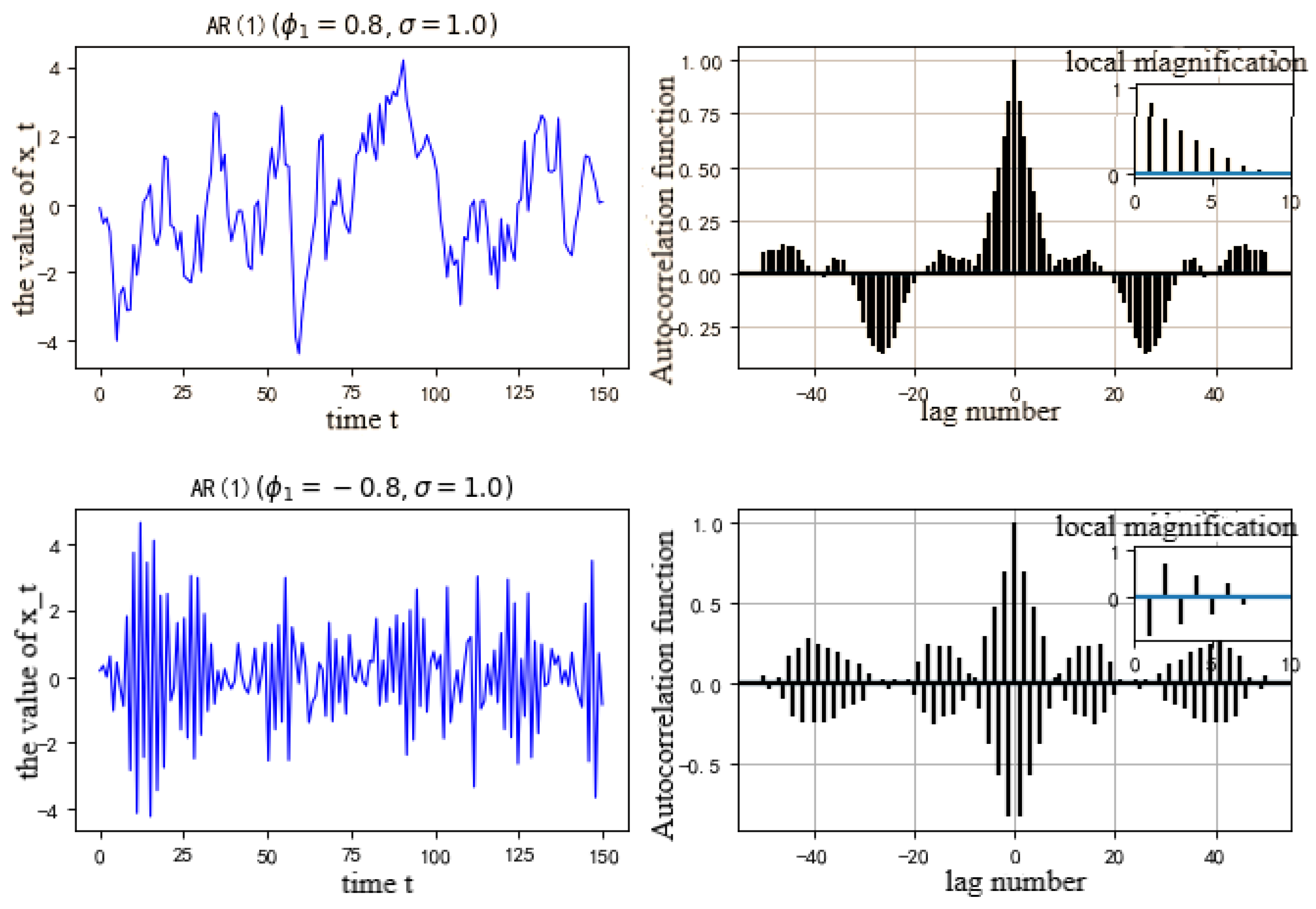
As shown in Figure 2 below, when $|{\varphi }_1|<1$, the absolute correlation between $X\left(t_i\right)$ and $X\left(t_j\right)$ of $X\left(t\right)$ at two different time points $t_i$ and $t_j$ approaches 0 when the time is increasing.

Figure 2. Example of an AR(1) process.

The above AR(1) process (7) is a special case of an OU process by taking ${\varphi }_1=1-\theta$ and $\mu =0$, that is,

$$X_{t+1}=X_t+\theta (\mu -X_t)+{ϵ}_{t+1},X_0={ϵ}_0.$$

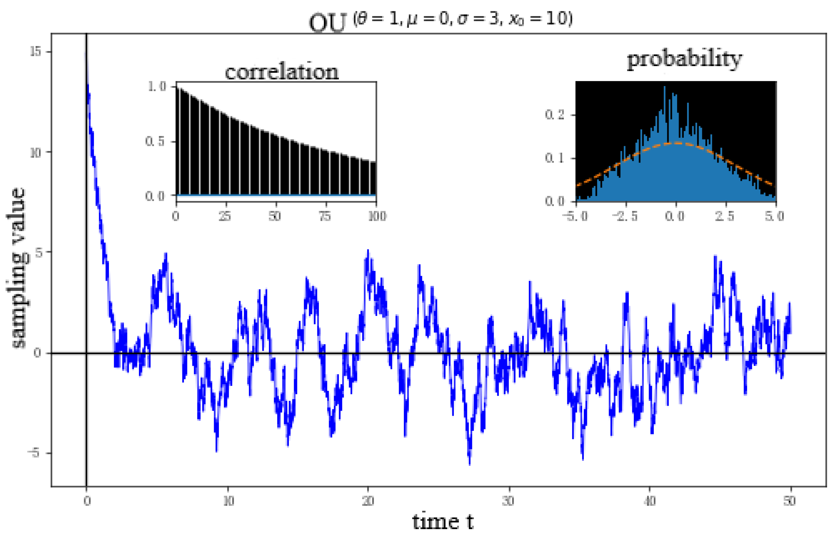
Therefore, the exponential covariance matrix constructed by the OU process can be used to describe the correlation in longitudinal data. An OU process is showed in Figure 3. It is obvious that when $X\left(t\right)$ moves toward its mean position with the increase in time t, the correlation between $X\left(t_i\right)$ and $X\left(t_j\right)$ at two different time points becomes weaker and weaker.

Figure 3. Example of an OU process.

4. Dirichlet Process and Dirichlet Process Mixture

4.1. Dirichlet Process

A Dirichlet process (DP) is a class of stochastic processes whose trace is a probability distribution. DP is often used in Bayesian inference to describe the prior knowledge of random variables.

Definition 1.

Given a measurable set $\mathcal{C}$, a basis distribution $G_0$, and a positive real number α, a Dirichlet process $\mathrm{DP}(G_0,\alpha )$ is a random process whose realization is a probability distribution on $\mathcal{C}$. For any measurable finite partition of $\mathcal{C}$, ${\left\{B_i\right\}}_{i=1}^n$, if $G\sim \mathrm{DP}(G_0,\alpha )$, then

$$(G\left(B_1\right),\dots ,G\left(B_n\right))\sim Dir(\alpha G_0\left(B_1\right),\dots ,\alpha G_0\left(B_n\right)).$$

where $Dir$ stands for the Dirichlet distribution. A DP is specified by the basis distribution $G_0$ and the concentration parameter α.

A DP can also be regarded as an infinite dimensional generalization of the n-dimensional Dirichlet distribution. A DP is the conjugate priori of an infinite, nonparametric discrete distribution. An important application of DP is to use it as a prior distribution for infinite mixture models. A statistically equivalent description of DP is based on the stick-breaking process, described as follows. Given a discrete distribution

$$G\left(\rho \right)=\sum _{i=1}^{\infty }{w}_k{\delta }_{{\rho }_k}\left(\rho \right)$$

where ${\delta }_{\rho k}$ is an indicator function, namely

$${\delta }_{{\rho }_k}=\left\{\begin{array}{cc}1,\hfill & \theta ={\rho }_k;\hfill \\ 0,\hfill & \theta \ne {\rho }_k.\hfill \end{array}\right.$$

${\rho }_k\stackrel{iid}{\sim }{G}_0,w_k=v_k{\prod }_{i=1}^{k-1}\left(1-v_i\right),v_i\stackrel{iid}{\sim }Beta(1,\alpha )$, the probability distribution G defined in this way is said to obey the Dirichlet process, denoted as $G\sim DP(G_0,\alpha )$. A DP can be constructed by a stochastic process. It possesses some advantages in its application in Bayesian model evaluation, density estimation, and mixed model clustering [20].

4.2. Dirichlet Process Mixture

We consider a set of i.i.d. sample data $\{y_1,\dots ,y_n\}$ as a part of an infinitely exchangeable sequence. $y_i$ follows the probability distribution $F(y;\mathit{\theta })$ with parameter $\mathit{\theta }\in \mathsf{\Theta }$, that is, $y_i|\mathit{\theta }\sim F(y;\mathit{\theta })$. It may be assumed that the prior distribution of $\mathit{\theta }$ is an unknown random probability measure G, and G can be constructed by DP, that is, $\mathit{\theta }|G\sim G$, $G\sim DP(G_0,\alpha )$. Thus, a Dirichlet process can be obtained using the hybrid (DPM) model definition:

$$y_i|\mathit{\theta }\sim F(y;\mathit{\theta }),\mathit{\theta }|G\sim G,G\sim \mathrm{DP}(G_0,\alpha ),$$

where $G_0$ and $\alpha$ are the basis distribution and model parameter, respectively. In general, the distributions F and $G_0$ will depend on additional hyperparameters not mentioned above. Since the trace of DP is discretized with probability 1, the above model can be regarded as a countably infinite mixture. We can integrate the distribution G in the above DPM to obtain the prior distribution of $\mathit{\theta }$:

$$\begin{array}{ccc}\hfill {\displaystyle {\theta }_i|({\theta }_1,\dots ,{\theta }_{i-1})}& \sim & {\displaystyle \frac{1}{\alpha +i-1}\sum _{j=1}^{i-1}{\delta }_{{\theta }_j}+\frac{\alpha }{\alpha +i-1}{G}_0}\hfill \\ \hfill & =& {\displaystyle \frac{i-1}{\alpha +i-1}\left(\frac{1}{i-1}\sum _{j=1}^{i-1}{\delta }_{{\theta }_j}\right)+\frac{\alpha }{\alpha +i-1}{G}_0,}\hfill \end{array}$$

where ${\delta }_{{\theta }_j}$ ($j=1,\dots ,i-1$, $i=2,3,\dots$) represents the point quality at ${\theta }_j$. This is a mixture of two distributions with weights $p=(i-1)/(\alpha +i-1)$ and $1-p=\alpha /(\alpha +i-1)$.

Let $\left\{f(·|\mathit{\theta }):\mathit{\theta }\in \mathsf{\Theta }\subset {\Re }^d\right\}$ be a family of density functions with parameter $\mathit{\theta }$. We assume that the density function of the observed data $y_i$ follows the probability distribution family $\mathcal{F}=\left\{f(·|G):G\in \mathcal{P}\right\}$ defined by

$$f\left(y_i\right|G)={\int }_{}f\left(y_i\right|\mathit{\theta })\mathrm{d}G\left(\mathit{\theta }\right),$$

(8)

which is called the DPM density of $y_i$, where $G\left(\mathit{\theta }\right)$ is the distribution of $\mathit{\theta }$. $\mathcal{F}$ is the nonparametric family of mixed distributions. The distribution G can be made random by assuming that G comes from a DP. In practice, to obtain the DPM density functions of $y_1,\dots ,y_n$, it is necessary to introduce the latent variable ${\theta }_i$ related to $y_i$. That is, after introducing ${\theta }_i$, the joint density function of $\{y_i:i=1,\dots ,n\}$ is ${\prod }_{i=1}^{n}f\left(y_i\right|{\theta }_i)$, where $\{{\theta }_i:i=1,\dots ,n\}$ is a sample from the distribution G. The joint density function of $\{y_i:i=1,\dots ,n\}$ can be expressed as ${\prod }_{i=1}^{n}f\left(y_i\right|G)$. We assign the prior distribution $DP(G_0,\alpha )$ to the distribution G with $G\sim DP(G_0,\alpha )$. The Bayesian model is set up as follows:

$$\begin{array}{cc}\hfill y_i|(\mathit{\beta },S_i,{\mathit{b}}_i,\mathit{\theta },\sigma )& \sim F(\mathit{\theta },\mathit{\beta },S_i,{\mathit{b}}_i,\sigma ),\hfill \\ \hfill {\theta }_k|G& \sim G,k=1,2,\dots \hfill \\ \hfill G(·)& =\sum _{k=1}^{\infty }{w}_k{\delta }_{{\theta }_k}(·),\hfill \end{array}\begin{array}{cc}\hfill w_k& ={\nu }_k\prod _{i=1}^{k-1}(1-{\nu }_i),\hfill \\ \hfill {\nu }_i& \stackrel{iid}{\sim }Beta(1,\alpha ),\hfill \\ \hfill {\theta }_k& \stackrel{iid}{\sim }{G}_0,k=1,2,\dots \hfill \end{array}$$

(9)

where $\{y_1,\dots ,y_n\}$ is a set of observations and $\{{\theta }_1,\dots ,{\theta }_n\}$ is a set of latent variables. Based on the discretization of DP, we can obtain the DPM density function of $S_i$ by

$$p\left(S_i\right|G)={\int }_{}^{}p\left(S_i\right|\theta )G\left(\mathrm{d}\theta \right)=\sum _{k=1}^{\infty }{w}_{k}p\left(S_i\right|{\theta }_k).$$

A semiparametric model can be set up by replacing the DP mixture on $\theta$ with the DP mixture on any subset of $\mathit{w}=\{w_k:k\ge 1\}$ (given by (9)), depending on $\theta$. Let ${\theta }_i=({\mathit{w}}_i,\eta )$ with a prior distribution $\eta$. The above DP mixture is only performed on the parameter ${\mathit{w}}_i$. The joint density function ${\prod }_{i=1}^{n}f\left(y_i\right|\eta ,G)$ of $\{y_i:i=1,\dots ,n\}$ can be obtained. The prior distribution of $\eta$ and G are prespecified. As a result, the semiparametric model can be determined [21].

5. Formulation of the Semiparametric Autoregressive Model

5.1. The Partial Dirichlet Process Mixture of Stochastic Process

The stochastic process in (1) is semiparameterized to generalize the general linear mixed model for longitudinal data. A nonparametric DP prior is assigned to the covariance parameter $({\sigma }_s^2,\rho )$ of ${\mathit{S}}_i$. To reduce the number of unknown parameters, a partial Dirichlet process mixture is performed on ${\mathit{S}}_i$, i.e., only a nonparametric DP prior is assigned to the parameter $\rho$. The semiparametric process is created as follows. First, we consider the OU process ${\mathit{S}}_i$ associated with object i to have a covariance matrix ${\mathit{C}}_i\left(\mathit{\theta }\right)={\sigma }_s^2{\tilde{\mathit{C}}}_i\left(\rho \right)$, where $\mathit{\theta }=({\sigma }_s^2,\rho )$. The $(k,l)$-element of the matrix ${\tilde{\mathit{C}}}_i\left(\rho \right)$ is given by ${\rho }^{|t_{il}-t_{ik}|}$. The matrix ${\tilde{\mathit{C}}}_i\left(\rho \right)$ associated with the random process ${\mathit{S}}_i$ has the following form:

$$\begin{array}{c}\hfill \left[\begin{array}{ccccc}1& {\rho }^{\left|t_{i2}-t_{i1}\right|}& {\rho }^{\left|t_{i3}-t_{i1}\right|}& \cdots & {\rho }^{\left|t_{i{n}_i}-t_{i1}\right|}\\ {\rho }^{\left|t_{i1}-t_{i2}\right|}& 1& {\rho }^{\left|t_{i3}-t_{i2}\right|}& \cdots & {\rho }^{\left|t_{i{n}_i}-t_{i2}\right|}\\ ⋮& ⋮& ⋮& & ⋮\\ {\rho }^{\left|t_{i1}-t_{i{n}_i}\right|}& {\rho }^{\left|t_{i2}-t_{i{n}_i}\right|}& {\rho }^{\left|t_{i3}-t_{i{n}_i}\right|}& \cdots & 1\end{array}\right];\end{array}$$

(10)

Second, we give the parameter $\rho$ a nonparametric DP prior:

$$\rho |G\sim G,G\sim \mathrm{DP}(G_0,\alpha ),$$

(11)

where $G_0$ is a known probability distribution, $\alpha$ is a constant, and the probability distribution G is generated by DP$(G_0,\alpha )$ satisfying

$$\begin{array}{cc}\hfill G(·)& =\sum _{k=1}^{\infty }{w}_k{\delta }_{{\varphi }_k}(·),\hfill \\ \hfill w_k& ={\nu }_k\prod _{i=1}^{k-1}(1-{\nu }_i),\hfill \end{array}\begin{array}{cc}\hfill {\nu }_i& \stackrel{iid}{\sim }Beta(1,\alpha ),\hfill \\ \hfill {\varphi }_k& \stackrel{iid}{\sim }{G}_0,\hfill \end{array}$$

(12)

where ${\delta }_{\varphi }(·)$ is the point quality of $\varphi$, and G is a random probability distribution.

Using the discretization of DP, for any parameter $\mathit{\varphi }$, we assume that $f(·|\mathit{\varphi })$ is a density function depending on the parameter $\mathit{\varphi }$. Let $\mathit{\varphi }|G\sim G$, $G\sim \mathrm{DP}(G_0,\alpha )$. The DPM density function can be obtained:

$$p(·|G)={\int }_{}^{}p(·|\mathit{\varphi })G\left(\mathrm{d}\mathit{\varphi }\right)=\sum _{k=1}^{\infty }{w}_{k}p(·|{\varphi }_k),$$

(13)

where ${\varphi }_k\stackrel{iid}{\sim }{G}_0$. After embedding the above conditional prior into the distribution of the random process ${\mathit{S}}_i$, we formulate the DPM model for ${\mathit{S}}_i$ as

$${\mathit{S}}_i|({\sigma }_s^2,\rho )\sim N(\mathit{0},{\sigma }_s^2{\tilde{\mathit{C}}}_i\left(\rho \right)),\hspace{1em}\rho |G\sim G,\hspace{1em}G\sim \mathrm{DP}(G_0,\alpha ).$$

(14)

Using the discretization of the distribution function G, we obtain the DPM density of the random process ${\mathit{S}}_i$ as follows.

$$p\left({\mathit{S}}_i\right|{\sigma }_s^2,G)={\int }_{}^{}N\left({\mathit{S}}_i\right|\mathit{0},{\sigma }_s^2{\tilde{\mathit{C}}}_i\left(\rho \right))\mathrm{d}G\left(\rho \right)=\sum _{k=1}^{\infty }{w}_{k}N\left({\mathit{S}}_i|\mathit{0},{\sigma }_s^2{\tilde{\mathit{C}}}_i\left({\tilde{\rho }}_k\right)\right).$$

(15)

This is an infinitely countable mixture of multivariate Gaussian density functions, where ${\tilde{\rho }}_k\stackrel{iid}{\sim }{G}_0$, $N(·|\mathit{0},{\sigma }_s^2{\tilde{\mathit{C}}}_i\left(\rho \right))$ represents a multivariate Gaussian density function with a zero-mean vector and a covariance matrix of ${\sigma }_s^2{\tilde{\mathit{C}}}_i\left(\rho \right)$. It can be seen that after the semiparametric treatment of the stochastic process ${\mathit{S}}_i$, its distribution is a mixture of stochastic processes, which is a more general mixture of OU processes.

Since G is discretized with probability 1, it provides an automatic clustering effect on the autocorrelation structure of the objects. After the OU process ${\mathit{S}}_i$ is semiparameterized, the covariance between any two time points $t_{il}$, $t_{ik}$ can be obtained by

$$\begin{array}{cc}\hfill & {\displaystyle \mathrm{cov}(s_i\left(t_{il}\right),s_i\left(t_{ik}\right)|{\sigma }_s^2,G)=\int \mathrm{cov}(s_i\left(t_{il}\right),s_i\left(t_{ik}\right)|{\sigma }_s^2,\rho )dG\left(\rho \right)}\hfill \\ \hfill =& {\displaystyle {\int }_{}^{}{\sigma }_s^2{\rho }^{|t_{il}-t_{ik}|}dG\left(\rho \right)=\sum _{k=1}^{\infty }{w}_k{\sigma }_s^2{\tilde{\rho }}_k^{|t_{il}-t_{ik}|}.}\hfill \end{array}$$

(16)

After semiparameterization of the OU process ${\mathit{S}}_i$, it not only contains an AR structure but also has an automatic clustering effect. If the observations $\{{\mathit{y}}_{\mathit{i}}:i=1,\dots ,n\}$ from model (1) are obtained at equal interval time points, the covariance matrix structure of ${\mathit{y}}_{\mathit{i}}$ becomes AR(1).

5.2. The Framework of a Hierarchical Model

We introduce potential parameters ${\rho }_1,{\rho }_2,\dots ,{\rho }_n$ (corresponding to n objects) and semiparameterize the general linear mixed model (1) with observations ${\mathit{y}}_1,{\mathit{y}}_2,\dots ,{\mathit{y}}_n$ satisfying the following model:

$$\begin{array}{cc}\hfill {\mathit{y}}_i& ={\mathit{X}}_i\mathit{\beta }+{\mathit{Z}}_i{\mathit{b}}_i+{\mathit{S}}_i+{ϵ}_i,\hfill \\ \hfill {\mathit{b}}_i|\tau & \sim N(\mathit{0},\mathit{D}(\tau \left)\right),\hfill \\ \hfill {\mathit{S}}_i|({\sigma }_s^2,{\rho }_i)& \sim N\left(\mathit{0},{\sigma }_s^2{\tilde{\mathit{C}}}_i\left({\rho }_i\right)\right),\hfill \end{array}\begin{array}{cc}\hfill {\rho }_i|G& \sim G,\hfill \\ \hfill G& \sim \mathrm{DP}(G_0,\alpha ),\hfill \\ \hfill {ϵ}_i& \sim N(\mathit{0},{\sigma }^2{\mathit{I}}_{n_i}).\hfill \end{array}$$

(17)

This is converted to a hierarchical model as follows:

$$\begin{array}{cc}\hfill {\mathit{y}}_i|(\mathit{\beta },{\mathit{b}}_i,{\mathit{S}}_i,{\sigma }^2)& \stackrel{ind}{\sim }N({\mathit{X}}_i\mathit{\beta }+{\mathit{Z}}_i{\mathit{b}}_i+{\mathit{S}}_i,{\sigma }^2\mathit{I}),\hfill \\ \hfill {\mathit{S}}_i|({\sigma }_s^2,{\rho }_i)& \stackrel{ind}{\sim }N\left(\mathit{0},{\sigma }_s^2{\tilde{\mathit{C}}}_i\left({\rho }_i\right)\right),\hfill \\ \hfill \{{\rho }_1,{\rho }_2,\dots ,{\rho }_n\}|G& \stackrel{iid}{\sim }G,\hfill \\ \hfill G& \sim \mathrm{DP}(G_0,\alpha ),\hfill \\ \hfill {\mathit{b}}_{\mathit{i}}|\tau & \stackrel{iid}{\sim }N(0,\mathit{D}\left(\tau \right)),\hfill \\ \hfill ({\sigma }^2,\mathit{\beta },\tau ,{\sigma }_s^2)& \sim p\left({\sigma }^2\right)\times N({\mathit{\beta }}_0,\mathit{B})\times p\left(\tau \right)\times p\left({\sigma }_s^2\right),\hfill \end{array}$$

(18)

where “ind” means independent only, ${\mathit{S}}_i$ and ${\mathit{b}}_i(1\le i\le n)$ are independent of each other, and $p\left({\sigma }^2\right)$, $N({\mathit{\beta }}_0,\mathit{B})$, $p\left(\tau \right)$, and $p\left({\sigma }_s^2\right)$ are the prior distributions of parameters ${\sigma }^2$, $\mathit{\beta }$, $\tau$, and ${\sigma }_s^2$, respectively. If $b_i$ is a scalar quantity corresponding to the random intercept of the model, we have $\tau ={\sigma }_b^2$. This model generalizes the exponential covariance function of the OU process. It realizes the automatic clustering effect between objects through parameter ${\rho }_i$. We call model (18) the Bayesian semiparametric autoregressive model, or simply the SPAR (semiparametric autoregressive) model.

Note that the SPAR model (18) is a parallel version of Quintana et al.’s [4] with additional conditions that the random effects $\{S_i:i=1,\dots ,n\}$ have a common variance component ${\sigma }_S^2$, and the autocorrelation parameters $({\rho }_1,{\rho }_2,\dots ,{\rho }_n)$ are assumed to be conditional i.i.d. with $DP(G_0,\alpha )$. This is different from model (3) in Quintana et al. [4], which assumes that the random-effect parameters $({\varphi }_1,\dots ,{\varphi }_n)$ are conditional i.i.d. with $DP(G_0,\alpha )$, where ${\varphi }_i=({\sigma }_i^2,{\rho }_i)$ with $var\left(S_i\right)={\sigma }_i^2{\tilde{\mathit{C}}}_i\left({\rho }_i\right)$ in our notation. The simpler assumptions help simplify the posterior inference. Quintana et al.’s [4] model assumptions do not lead to explicit posterior distributions of model parameters. Their posterior inference on model parameters may have to be performed by nonparametric MCMC algorithms. Because no explicit expressions related to posterior inference on model parameters are given by [4], we are not able to conclude if Quintana et al.’s [4] Bayesian posterior inference is a complete semiparametric MCMC method or a combination of semiparametric and nonparametric MCMC methods. By imposing simpler assumptions on the parameters in model (18), we are able to obtain the explicit posterior distributions of all model parameters in the subsequent context and conclude that our approach to handling the SPAR model (18) is a complete semiparametric MCMC method.

In the SPAR model (18), the random process part is an OU process mixture. The correlation matrix ${\tilde{\mathit{C}}}_i\left({\rho }_i\right)$ possesses the following form:

$$\begin{array}{c}\hfill {\tilde{\mathit{C}}}_i\left({\rho }_i\right)=\left[\begin{array}{ccccccc}1& {\rho }_i^{|t_{i2}-t_{i1}|}& {\rho }_i^{|t_{i3}-t_{i1}|}& \cdots & {\rho }_i^{|t_{il}-t_{i1}|}& \cdots & {\rho }_i^{|t_{i{n}_i}-t_{i1}|}\\ {\rho }_i^{|t_{i1}-t_{i2}|}& 1& {\rho }_i^{|t_{i3}-t_{i2}|}& \cdots & {\rho }_i^{|t_{il}-t_{i2}|}& \cdots & {\rho }_i^{|t_{i{n}_i}-t_{i2}|}\\ ⋮& ⋮& ⋮& & ⋮& & ⋮\\ {\rho }_i^{|t_{i1}-t_{ik}|}& {\rho }_i^{|t_{i2}-t_{ik}|}& {\rho }_i^{|t_{k3}-t_{ik}|}& \cdots & {\rho }_i^{|t_{il}-t_{ik}|}& \cdots & {\rho }_i^{|t_{i{n}_i}-t_{ik}|}\\ ⋮& ⋮& ⋮& & ⋮& & ⋮\\ {\rho }_i^{|t_{i1}-t_{i{n}_i}|}& {\rho }_i^{|t_{i2}-t_{i{n}_i}|}& {\rho }_i^{|t_{i3}-t_{i{n}_i}|}& \cdots & {\rho }_i^{|t_{il}-t_{i{n}_i}|}& \cdots & 1\end{array}\right].\end{array}$$

(19)

Using the property of the OU process structure, ${\tilde{\mathit{C}}}_i\left({\rho }_i\right)$ can be analyzed backwards. The inverse matrix of ${\tilde{\mathit{C}}}_i\left({\rho }_i\right)$ is a tridiagonal. Denote by $r_{ik}={\rho }_i^{|t_{i,k+1}-t_{ik}|}$ ($k=1,2,\dots ,n_i-1$). We have the $(k,l)$-th element of ${\tilde{\mathit{C}}}_i\left({\rho }_i\right)$ given by

$${\left\{{\tilde{\mathit{C}}}_i\left({\rho }_i\right)\right\}}_{kl}={\rho }_i^{|t_{il}-t_{ik}|}={\rho }_i^{|t_{i,k+1}-t_{ik}|+|t_{i,k+2}-t_{i,k+1}|+\cdots +|t_{il}-t_{i,l-1}|}=r_{ik}{r}_{i,k+1}\dots r_{i,l-1}.$$

(20)

So, ${\tilde{\mathit{C}}}_i\left({\rho }_i\right)$ can be rewritten as

$$\begin{array}{c}\hfill \left[\begin{array}{ccccccc}1& r_{i1}& r_{i1}{r}_{i2}& \cdots & r_{i1}\dots r_{i,l-1}& \cdots & r_{i1}\dots r_{i,n_i-1}\\ r_{i1}& 1& r_{i2}& \cdots & r_{i2}\dots r_{i,l-1}& \cdots & r_{i2}\dots r_{i,n_i-1}\\ ⋮& ⋮& ⋮& & ⋮& ⋮& ⋮\\ r_{i1}\dots r_{i,k-1}& r_{i2}\dots r_{i,k-1}& r_{i3}\dots r_{i,k-1}& \cdots & r_{ik}\dots r_{i,l-1}& \cdots & r_{ik}\dots r_{i,n_i-1}\\ ⋮& ⋮& ⋮& & ⋮& ⋮& ⋮\\ r_{i1}\dots r_{i,n_i-1}& r_{i2}\dots r_{i,n_i-1}& r_{i3}\dots r_{i,n_i-1}& \cdots & r_{il}\dots r_{i,n_i-1}& \cdots & 1\end{array}\right].\end{array}$$

Using the correlation theory of the anticorrelation random variables [22], we can compute the elements of the inverse matrix ${\tilde{\mathit{C}}}_i^{-1}\left({\rho }_i\right)$ of ${\tilde{\mathit{C}}}_i\left({\rho }_i\right)$ as follows:

$$\begin{array}{ccc}\hfill {\displaystyle {\left\{{\tilde{\mathit{C}}}_i^{-1}\left({\rho }_i\right)\right\}}_{11}}& =& {\displaystyle \frac{1}{1-r_{i1}^2},}\hfill \\ \hfill {\displaystyle {\left\{{\tilde{\mathit{C}}}_i^{-1}\left({\rho }_i\right)\right\}}_{kk}}& =& {\displaystyle \frac{1-r_{i,k-1}^2{r}_{ik}^2}{1-r_{i,k-1}^2-r_{ik}^2+r_{i,k-1}^2{r}_{ik}^2},k=2,3,\dots ,n_i-1,}\hfill \\ \hfill {\displaystyle {\left\{{\tilde{\mathit{C}}}_i^{-1}\left({\rho }_i\right)\right\}}_{kk+1}}& =& {\displaystyle -\frac{r_{ik}}{1-r_{ik}^2},k=1,2,\dots ,n_i-1,}\hfill \\ \hfill {\displaystyle {\left\{{\tilde{\mathit{C}}}_i^{-1}\left({\rho }_i\right)\right\}}_{n_i{n}_i}}& =& {\displaystyle \frac{1}{1-r_{i,n_i-1}^2}.}\hfill \end{array}$$

(21)

${\tilde{\mathit{C}}}_i^{-1}\left({\rho }_i\right)$ turns out to be a tridiagonal matrix.

The random process corresponding to the i-th object ${\mathit{S}}_i={(s_{i1},s_{i2},\dots ,s_{i{n}_i})}^{\prime }$ satisfies the conditional distribution:

$${\mathit{S}}_i|{\sigma }_s^2,{\rho }_i\sim N_{n_i}\left(\mathit{0},{\sigma }_s^2{\tilde{\mathit{C}}}_i\left({\rho }_i\right)\right).$$

So, the conditional density function is

$$f\left({\mathit{S}}_i\right|{\sigma }_s^2,{\rho }_i)=f(s_{i1},\dots ,s_{i{n}_i}|{\sigma }_s^2,{\rho }_i)=f\left(s_{i1}\right|{\sigma }_s^2,{\rho }_i)\cdots f\left(s_{i{n}_i}\right|s_{i1},\dots ,s_{i,n_i-1},{\sigma }_s^2,{\rho }_i).$$

(22)

When the inverse matrix of the covariance matrix ${\tilde{\mathit{C}}}_i\left({\rho }_i\right)$ of the random process ${\mathit{S}}_i$ has the above tridiagonal form, based on the property of the multivariate normal distribution, the conditional density function $f\left({\mathit{S}}_i\right|{\sigma }_s^2,{\rho }_i)$ of ${\mathit{S}}_i$ can be decomposed into the product of $n_i$ univariate Gaussian density functions as follows:

$$\begin{array}{cc}\hfill s_{i1}& \sim N(0,{\sigma }_s^2),\hfill \\ \hfill s_{i2}|(s_{i1}={\tilde{s}}_1)& \sim N\left({\tilde{s}}_1{r}_{i1},{\sigma }_s^2(1-r_{i1}^2)\right),\hfill \\ \hfill ⋮\\ \hfill s_{ik}|(s_{i1}={\tilde{s}}_1,\dots ,s_{i,k-1}={\tilde{s}}_{k-1})& \sim N\left({\tilde{s}}_{k-1}{r}_{i,k-1},{\sigma }_s^2(1-r_{i,k-1}^2)\right),\hfill \\ \hfill ⋮\\ \hfill s_{i{n}_i}|(s_{i1}={\tilde{s}}_1\dots ,s_{i,n_i-1}={\tilde{s}}_{n_i-1})& \sim N\left({\tilde{s}}_{n_i-1}{r}_{i,n_i-1},{\sigma }_s^2(1-r_{i,n_i-1}^2)\right).\hfill \end{array}$$

(23)

It is known that $r_{ik}={\rho }_i^{|t_{i,k+1}-t_{ik}|},k=1,2,\dots ,n_i-1$. Hence,

$$\begin{array}{cc}\hfill s_{i1}& \sim N(0,{\sigma }_s^2),\hfill \\ \hfill s_{i2}|(s_{i1}={\tilde{s}}_1)& \sim N\left({\tilde{s}}_1{\rho }^{|t_{i2}-t_{i1}|},{\sigma }_s^2\left(1-{\rho }^{2|t_{i2}-t_{i1}|}\right)\right),\hfill \\ \hfill ⋮\\ \hfill s_{ik}|(s_{i,k-1}={\tilde{s}}_{k-1})& \sim N\left({\tilde{s}}_{k-1}{\rho }_i^{|t_{ik}-t_{i,k-1}|},{\sigma }_s^2\left(1-{\rho }_i^{2|t_{ik}-t_{i,k-1}|}\right)\right),\hfill \\ \hfill ⋮\\ \hfill s_{i{n}_i}|(s_{i,n_i-1}={\tilde{s}}_{n_i-1})& \sim N\left({\tilde{s}}_{n_i-1}{\rho }_i^{|t_{i{n}_i}-t_{i,n_i-1}|},{\sigma }_s^2\left(1-{\rho }_i^{2|t_{i{n}_i}-t_{i,n_i-1}|}\right)\right).\hfill \end{array}$$

(24)

As a result, the conditional density function of ${\mathit{S}}_i$ in the random process $f\left({\mathit{S}}_i\right|{\sigma }_s^2,{\rho }_i)$ can be decomposed as follows:

$$\begin{array}{cc}\hfill f\left({\mathit{S}}_i\right|{\sigma }_s^2,{\rho }_i)=& N\left(s_{i1}|0,{\sigma }_s^2\right)\cdots N\left(s_{ik}|{\tilde{s}}_{k-1}{\rho }_i^{|t_{ik}-t_{i,k-1}|},{\sigma }_s^2\left(1-{\rho }_i^{2|t_{ik}-t_{i,k-1}|}\right)\right)\cdots \hfill \\ \hfill & N\left(s_{i{n}_i}|{\tilde{s}}_{n_i-1}{\rho }_i^{|t_{i{n}_i}-t_{i,n_i-1}|},{\sigma }_s^2\left(1-{\rho }_i^{2|t_{i{n}_i}-t_{i,n_i-1}|}\right)\right).\hfill \end{array}$$

(25)

The above decomposition greatly simplifies the computation of the distribution of the random process ${\mathit{S}}_i$, which can be obtained by direct computation of the distribution of a single Gaussian variable.

6. The Marginal Likelihood, Prior Determination, and Posteriori Inference

Let $\mathit{y}=({\mathit{y}}_1,{\mathit{y}}_2,\dots ,{\mathit{y}}_n)$, $\mathit{b}=({\mathit{b}}_1,{\mathit{b}}_2,\dots ,{\mathit{b}}_n)$, $\mathit{S}=({\mathit{S}}_1,{\mathit{S}}_2,\dots ,{\mathit{S}}_n)$, and $\rho =({\rho }_1,{\rho }_2,\dots ,{\rho }_n)$. Denote by $\mathbf{\Psi }=(\mathit{\beta },{\sigma }^2,{\sigma }_s^2,\rho ,\tau )$, which represents the parameter vector in model (18). A random process that specifies the AR structure in the SPAR model (18) is

$${\mathit{S}}_i|{\sigma }_s^2,{\rho }_i\sim N\left(\mathit{0},{\sigma }_s^2{\tilde{\mathit{C}}}_i\left({\rho }_i\right)\right),{\rho }_i|G\sim G_0,G\sim \mathrm{DP}(G_0,\alpha ).$$

(26)

The marginal distribution of the covariance parameter ${\rho }_i$ can be obtained from the joint distribution of all terms in (26) as follows:

$${\rho }_1\sim G_0,{\rho }_i|({\rho }_1,{\rho }_2,\dots ,{\rho }_{i-1})\sim \frac{\alpha }{\alpha +i-1}{G}_0+\frac{1}{\alpha +i-1}\sum _{k=1}^{i-1}{\delta }_{{\rho }_k}$$

(27)

for $i=2,\dots ,n$. We assume that $\{{\mathit{S}}_1,{\mathit{S}}_2,\dots ,{\mathit{S}}_n\}$ is a sample from the multivariate Gaussian distribution. It can be regarded as a part of an exchangeable sequence. By using the exchangeable property, the corresponding order i of the observation ${\mathit{y}}_i$ can be considered as the last one in all n observations from n objects. Then, ${\mathit{y}}_i$ is the corresponding vector $S_i$. Or we can consider it as the last one that gives us ${\rho }_{(-i)}$. The conditional prior score of ${\rho }_i$ is

$$\begin{array}{c}\hfill {\rho }_i|{\rho }_{(-i)}\sim \frac{\alpha }{\alpha +i-1}{G}_0+\frac{1}{\alpha +i-1}\sum _{k\ne i}{\delta }_{{\rho }_k},\end{array}$$

(28)

where ${\rho }_{(-i)}$ represents all other $\rho$’s except ${\rho }_i$. According to the product formula, we have

$$p\left(\mathit{\rho }\right)=p({\rho }_1,{\rho }_2,\dots ,{\rho }_n)=p\left({\rho }_1\right)p\left({\rho }_2\right|{\rho }_1)\cdots p\left({\rho }_n\right|{\rho }_1,{\rho }_2,\dots ,{\rho }_{n-1}).$$

Based on the above conditional prior distributions, we can obtain the prior distribution $p\left(\mathit{\rho }\right)$ of parameter $\mathit{\rho }$. Compute the likelihood function of the SPAR model (18) as follows:

$$\begin{array}{cc}\hfill \mathit{L}\left(\mathbf{\Psi }\right|\mathit{y},\mathit{b},\mathit{S})& =f(\mathit{y},\mathit{b},\mathit{S}|\mathbf{\Psi })\hfill \\ \hfill & =f\left(\mathit{y}\right|\mathit{b},\mathit{S},\mathbf{\Psi }\left)f\right(\mathit{b}\left|\mathbf{\Psi }\right)f\left(\mathit{S}\right|\mathbf{\Psi })\hfill \\ \hfill & =f\left(\mathit{y}\right|\mathit{b},\mathit{S},\mathit{\beta },{\sigma }^2)f\left(\mathit{b}\right|\tau )f\left(\mathit{S}\right|{\sigma }_s^2,\rho ).\hfill \end{array}$$

(29)

Let

$$p\left(\mathbf{\Psi }\right)=p(\mathit{\beta },{\sigma }^2,{\sigma }_s^2,\mathit{\rho },\mathit{\tau })=p\left(\mathit{\beta }\right)p\left({\sigma }^2\right)p\left({\sigma }_s^2\right)p\left(\rho \right)p\left(\tau \right),$$

This implies that the prior distributions of each parameter are independent of each other. The joint posterior of the SPAR model is computed as follows:

$$\begin{array}{cc}\hfill p(\mathbf{\Psi },\mathit{b},\mathit{S}|\mathit{y})& \propto p(\mathit{y},\mathit{b},\mathit{S}|\mathbf{\Psi }\left)p\right(\mathbf{\Psi })\hfill \\ \hfill & =\left\{\prod _{i=1}^{n}f({\mathit{y}}_i,{\mathit{b}}_i,{\mathit{S}}_i|\mathbf{\Psi })\right\}p\left(\mathbf{\Psi }\right)\hfill \\ \hfill & =\left\{\prod _{i=1}^{n}f\left({\mathit{y}}_i|\mathit{\beta },{\mathit{S}}_i,{\mathit{b}}_i,{\sigma }^2\right)f\left({\mathit{b}}_i\right|\tau )f\left({\mathit{S}}_i|{\sigma }_s^2,{\rho }_i\right)\right\}p\left(\mathbf{\Psi }\right).\hfill \end{array}$$

(30)

That is, the joint posterior distribution is the product of the likelihood function and the prior distribution. The first term of the likelihood function is the density function of the estimated n-dimensional Gaussian distribution $N({\mathit{X}}_i\mathit{\beta }+{\mathit{Z}}_i{\mathit{b}}_i+{\mathit{S}}_i,{\sigma }^2\mathit{I})$ at ${\mathit{y}}_i$. The second term is in ${\mathit{b}}_i$, the density function of the estimated q-dimensional Gaussian distribution $N(\mathit{0},\mathit{D}(\tau \left)\right)$. The third term is the product of the $n_i$ univariate Gaussian distribution density functions.

To estimate the joint posterior distribution of the SPAR model (18), it is necessary to use the Bayesian theorem to obtain the conditional distribution of parameters in the model:

$$\begin{array}{cc}\hfill & p\left(\mathit{\beta }\right|\mathit{y},\mathit{b},\mathit{S},{\sigma }^2,{\sigma }_s^2,\mathit{\rho },\mathit{\tau }),\hfill \\ \hfill & p\left({\mathit{b}}_i\right|\mathit{y},\mathit{\beta },{\mathit{b}}_{-i},\mathit{S},{\sigma }^2,{\sigma }_s^2,\mathit{\rho },\mathit{\tau }),\hfill \\ \hfill & p\left({\mathit{S}}_i\right|\mathit{y},\mathit{\beta },\mathit{b},{\mathit{S}}_{-i},{\sigma }^2,{\sigma }_s^2,\mathit{\rho },\mathit{\tau }),\hfill \end{array}\begin{array}{cc}\hfill & p\left({\sigma }^2\right|\mathit{y},\mathit{\beta },\mathit{b},\mathit{S},{\sigma }_s^2,\mathit{\rho },\mathit{\tau }),\hfill \\ \hfill & p\left({\sigma }_s^2\right|\mathit{y},\mathit{\beta },\mathit{b},\mathit{S},{\sigma }^2,\mathit{\rho },\mathit{\tau }),\hfill \\ \hfill & p\left({\rho }_i\right|\mathit{y},\mathit{\beta },\mathit{b},\mathit{S},{\sigma }^2,{\sigma }_s^2,{\rho }_{-i},\mathit{\tau }),\hfill \\ \hfill & p\left(\tau \right|\mathit{y},\mathit{\beta },\mathit{b},\mathit{S},{\sigma }^2,{\sigma }_s^2,\mathit{\rho }).\hfill \end{array}$$

(31)

The MCMC algorithm is employed to estimate these conditional distributions. The conditional distribution of a parameters is denoted by $p(·|\ast )$ in the subsequent context.

7. A Monte Carlo Study

7.1. Simulation Design

To verify that the SPAR model (18) can effectively simulate the correlation structure in the longitudinal data, the empirical sample data were generated under the four situations of zero mean and covariance structure being compound symmetric (CS), autoregressive (AR), mixed CS and AR, and nonstructured, respectively. The MCMC method was employed to estimate the covariance matrix and the correlation matrix in the four different cases, respectively, and compared with the traditional Bayesian inverse-Wishart estimation method.

Consider a brief form of the SPAR model (18):

$$\begin{array}{c}\hfill {\mathit{y}}_i=(\mathit{\beta }+b_i)e+{\mathit{S}}_i+{ϵ}_i,\end{array}$$

(32)

where $\mathit{\beta }$ represents a fixed intercept, e is an $n_i\times 1$ vector of ones, $b_i\sim N(0,{\sigma }_b^2)$ is a random intercept, and ${\mathit{S}}_i$ is an OU process corresponding to ${\mathit{y}}_i$. Convert the above model into a hierarchical model:

$$\begin{array}{cc}\hfill {\mathit{y}}_i|(\mathit{\beta },b_i,{\mathit{S}}_i,{\sigma }^2)& \stackrel{ind}{\sim }N\left((\mathit{\beta }+b_i)e+{\mathit{S}}_i,{\sigma }^2\mathit{I}\right),\hfill \\ \hfill {\mathit{S}}_i|({\sigma }_s^2,{\rho }_i)& \stackrel{ind}{\sim }N\left(\mathit{0},{\sigma }_s^2\tilde{\mathit{C}}\left({\rho }_i\right)\right),\hfill \\ \hfill \{{\rho }_1,{\rho }_2,\dots ,{\rho }_n\}|G& \stackrel{iid}{\sim }G,\hfill \\ \hfill G& \sim \mathrm{DP}(G_0,\alpha ),\hfill \end{array}\begin{array}{cc}\hfill b_i& \stackrel{iid}{\sim }N(0,{\sigma }_b^2),\hfill \\ \hfill \mathit{\beta }& \sim N({\mu }_0,{\sigma }_0^2),\hfill \\ \hfill {\sigma }^2& \sim IG({\alpha }_0,{\mathit{\beta }}_0),\hfill \\ \hfill {\sigma }_s^2& \sim IG({\alpha }_1,{\mathit{\beta }}_1).\hfill \end{array}$$

(33)

For the special case of balanced sample design with $n_i=m$ ($i=1,2,\dots ,n$) and $t_{ij}=t_j$ for $i=1,2,\dots ,n$, the joint posterior distribution of model (18) can be easily computed by

$$\begin{array}{cc}\hfill & {\displaystyle p(\mathit{\beta },{\sigma }^2,{\sigma }_s^2,\mathit{\rho },\mathit{b},\mathit{S}|\mathit{y})=\frac{p\left(\mathit{y}\right|\mathit{\beta },\mathit{b},\mathit{S},{\sigma }^2)p\left(\mathit{b}\right)p\left(\mathit{S}\right|{\sigma }_s^2,\mathit{\rho })p(\mathit{\beta },{\sigma }^2,{\sigma }_s^2,\mathit{\rho })}{p\left(\mathit{y}\right)}}\hfill \\ \hfill \propto & {\displaystyle p\left(\mathit{y}\right|\mathit{\beta },\mathit{b},\mathit{S},{\sigma }^2)p\left(\mathit{b}\right)p\left(\mathit{S}\right|{\sigma }_s^2,\mathit{\rho })p(\mathit{\beta },{\sigma }^2,{\sigma }_s^2,\mathit{\rho })}\hfill \\ \hfill =& {\displaystyle \left\{\prod _{i=1}^{n}f\left({\mathit{y}}_i|\mathit{\beta },b_i,{\mathit{S}}_i,{\sigma }^2\right)f\left(b_i\right)f\left({\mathit{S}}_i|{\sigma }_s^2,{\rho }_i\right)\right\}p\left(\mathit{\beta }\right)p\left({\sigma }^2\right)p\left({\sigma }_s^2\right)p\left(\mathit{\rho }\right).}\hfill \end{array}$$

(34)

To realize the Bayesian inference of the model, it is necessary to use the Bayesian theorem to obtain the conditional distribution of each parameter. The lengthy derivations of all conditional probability distributions are given in the Appendix A at the end of the paper.

Performing a posteriori inference on the covariance matrix $\mathbf{\Sigma }=\left({\sigma }_{ij}\right)$ ($m\times m$) is equivalent to estimating the posteriori mean of $\mathbf{\Sigma }$:

$$\widehat{\mathbf{\Sigma }}=E\left\{\mathbf{\Sigma }|\mathit{y}\right\}=E\left\{{\sigma }_b^2\mathit{A}+{\sigma }_s^2\tilde{\mathit{C}}\left(\rho \right)+{\sigma }^2\mathit{I}|\mathit{y}\right\},\hspace{1em}m\times m$$

(35)

where $\mathit{A}=e{e}^{\prime }$. The posteriori estimate for the correlation matrix $\mathit{R}$ can be obtained by using $\widehat{\mathbf{\Sigma }}$ to calculate the estimated $\widehat{\mathit{R}}$ of the correlation matrix $\mathit{R}$:

$$\widehat{\mathit{R}}={\mathit{R}}_0\widehat{\mathbf{\Sigma }}{\mathit{R}}_0,\hspace{1em}{\mathit{R}}_0=diag\left({\widehat{\sigma }}_{11}^{-\frac{1}{2}},\dots ,{\widehat{\sigma }}_{mm}^{-\frac{1}{2}}\right),\hspace{1em}\widehat{\mathbf{\Sigma }}=\left({\widehat{\sigma }}_{ij}\right):m\times m.$$

(36)

The mean square error loss function is used to evaluate the performance of the posterior mean:

$$MSE\left(\mathbf{\Sigma }\right)={\left(\frac{1}{m^2}\sum _{i=1}^m\sum _{j=1}^m{({\widehat{\sigma }}_{ij}-{\sigma }_{ij})}^2\right)}^{\frac{1}{2}}.$$

(37)

Compared with the Bayesian estimates of the covariance matrix and correlation matrix under other loss functions [23], the most common one is the entropy loss function defined by

$$\begin{array}{c}\hfill L_1(\widehat{\mathbf{\Sigma }},\mathbf{\Sigma })=\mathrm{tr}\left(\widehat{\mathbf{\Sigma }}{\mathbf{\Sigma }}^{-1}\right)-\log \left|\widehat{\mathbf{\Sigma }}{\mathbf{\Sigma }}^{-1}\right|-m.\end{array}$$

(38)

The quadratic loss function is given by

$$\begin{array}{c}\hfill L_2(\widehat{\mathbf{\Sigma }},\mathbf{\Sigma })=\mathrm{tr}{(\widehat{\mathbf{\Sigma }}{\mathbf{\Sigma }}^{-1}-I)}^2.\end{array}$$

(39)

The Bayesian estimates of the covariance matrices based on the loss functions $L_1(\widehat{\mathbf{\Sigma }},\mathbf{\Sigma })$ and $L_2(\widehat{\mathbf{\Sigma }},\mathbf{\Sigma })$ are given by

$$\widehat{\mathbf{\Sigma }}={\left[E\left({\mathbf{\Sigma }}^{-1}|\mathit{y}\right)\right]}^{-1}\hspace{1em}\mathrm{and}\hspace{1em}\mathrm{vec}\left(\widehat{\mathbf{\Sigma }}\right)={\left[E\left({\mathbf{\Sigma }}^{-1}\otimes {\mathbf{\Sigma }}^{-1}|\mathit{y}\right)\right]}^{-1}\mathrm{vec}\left[E\left({\mathbf{\Sigma }}^{-1}|\mathit{y}\right)\right],$$

(40)

respectively, where vec stands for the column vectorization of a matrix, and “⊗” denotes the Kronecker product of matrices. Similarly, the Bayesian estimate of correlation moment $\mathit{R}$ under various loss functions can be obtained.

7.2. Simulation Specification and Display of Empirical Results

In the simulation, we firstly set up the four different covariance structures as in the following Equations (41) and the priors as given in the following Equations (43)–(46). Then, we run the MCMC training trial 2000 times. After seeing the convergence trend approach relative stability after 2000 training trials, we generated 20 datasets consisting of 100 sample points of length 6 for each object. This is equivalent to the longitudinal data structure in Table 1, with $n=100$, $p=6$, and $k=1$ for each generated longitudinal dataset.

The four covariance matrices are designed as follows:

$$\begin{array}{cc}\hfill {\mathbf{\Sigma }}_1(i,j)& =10I(i=j)+7I(i\ne j)\hfill \\ \hfill {\mathbf{\Sigma }}_2(i,j)& =10\times 0.4^{|i-j|}\hfill \\ \hfill {\mathbf{\Sigma }}_3(i,j)& =0.3{\mathbf{\Sigma }}_1(i,j)+0.7{\mathbf{\Sigma }}_2(i,j)\hfill \\ \hfill {\mathbf{\Sigma }}_4(i,j)& =\frac{10}{\sqrt{1+|i-j|}}.\hfill \end{array}$$

(41)

The root mean square error (RMSE) for estimating $\mathbf{\Sigma }$ is computed by

$$RMSE=\frac{1}{20}\sum _{k=1}^{20}\mathrm{MSE},\hspace{1em}MSE=\sqrt{\frac{1}{36}\sum _{i=1}^6\sum _{j=1}^6{({\mathbf{\Sigma }}_{ij}-{\widehat{\mathbf{\Sigma }}}_{ij})}^2}.$$

(42)

The RMSE for estimating the correlation matrix $\mathit{R}$ is computed similarly.

For each of the four different covariance structures, we used the R-package (called Pandas, available upon request) to perform a preliminary analysis on the simulated data with a specified prior distribution, respectively. Then, we employed the MCMC algorithm to perform the sampling estimation on each parameter in the model. We used the three methods mentioned before to perform the convergence assessment on the sampling results. Finally, we obtained the estimates for the four types of covariance and correlation matrices. The estimation error was computed based on three types of loss functions. The inverse-Wishart estimation error was also obtained for comparison.

For the case of the CS covariance structure, the prior distribution of the parameter in the model is specified as follows:

$$\begin{array}{cc}\hfill G_0=N& (0,10),\alpha =0.75,\hfill \\ \hfill b_i& \stackrel{iid}{\sim }N(0,7),\hfill \end{array}\begin{array}{cc}\hfill \mathit{\beta }& \sim N(0,25),\hfill \\ \hfill {\sigma }^2& \sim IG(3,2),\hfill \\ \hfill {\sigma }_s^2& \sim IG(6,10).\hfill \end{array}$$

(43)

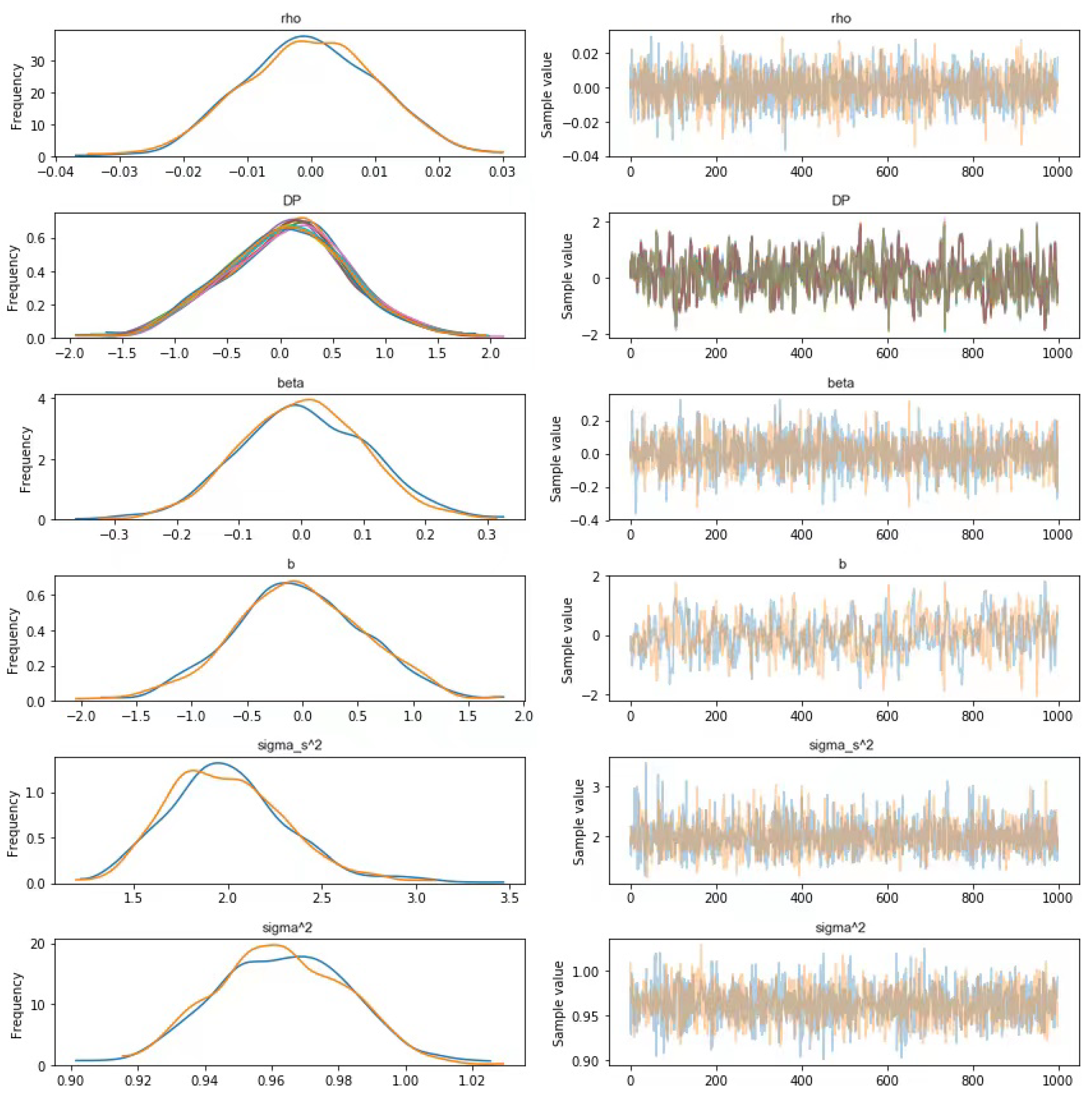
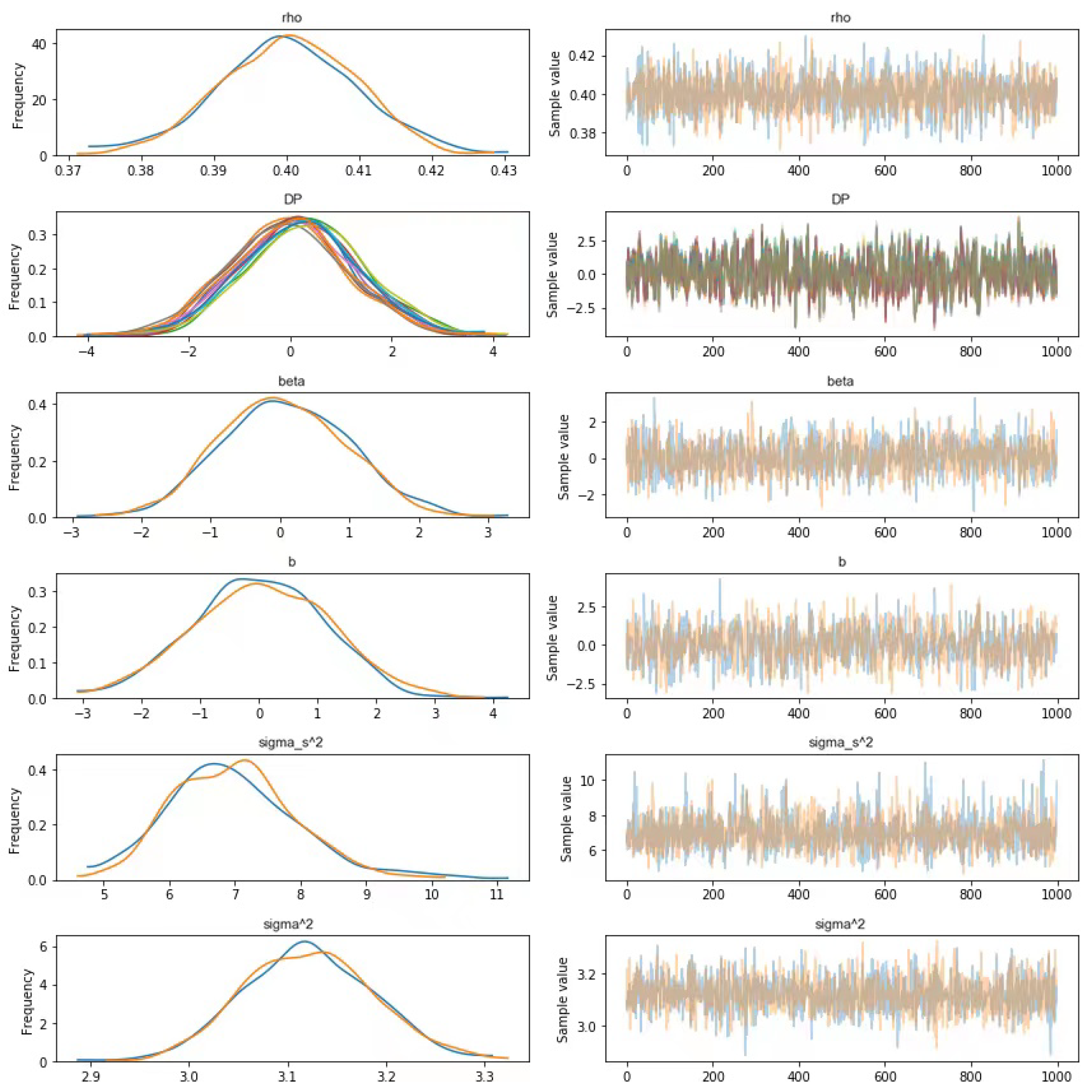
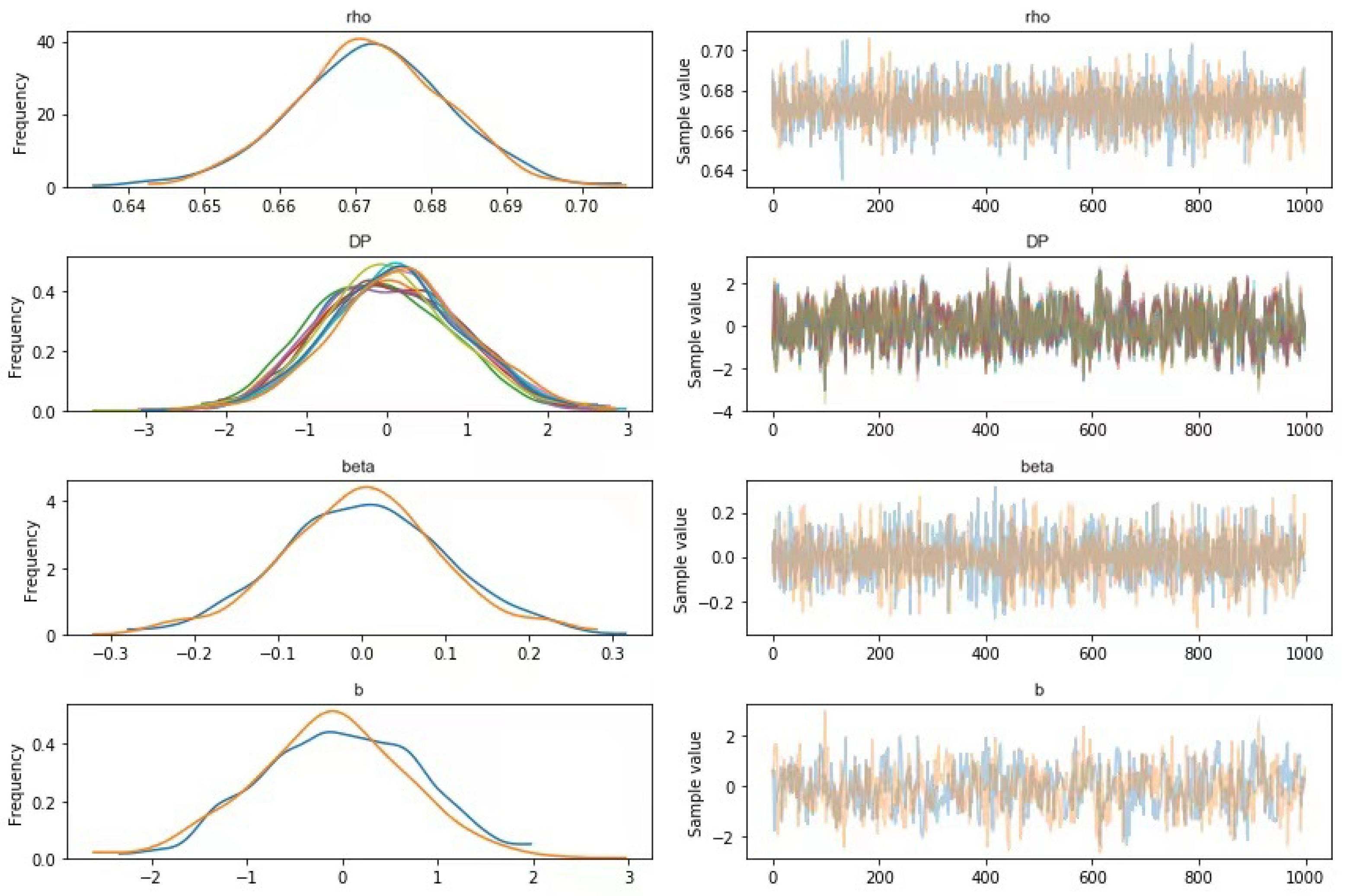
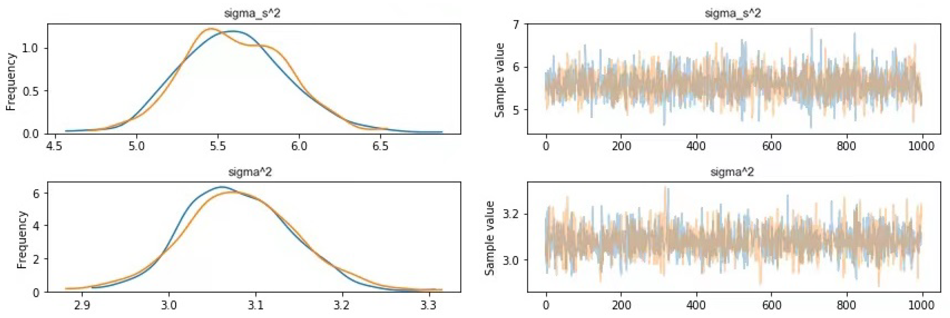
Each parameter in the model is sampled and estimated using the MCMC method. The last 1000 iterations were taken to draw the posterior sampling trend diagram, as shown in Figure 4.

Figure 4. Sampling results under the CS structure: The left panel gives the sampling distributions (smoothed by the kernel density estimation) for the parameters and the DP, which contain six pairs of DPs (each subject is observed for $p=6$ variables in the simulation), each pair consisting of a DP generated from model (18) with the CS structure and a DP generated from the traditional model with the inverse-Wishart structure (sampling population specified by Equations (23), (24) and (43)). The orange line stands for sampling distribution under the SPAR model (18), and the blue line for the inverse-Wishart model; the right panel gives the the graphs of two Markov chains under the SPAR model (orange) and the inverse-Wishart model (blue), respectively, as well as the Markov chain for each individual DP (different color for each). Each graph in the right column shows the relationship between each estimated parameter (the ordinate) versus the number of random samples in the abscissa, ranging from 1 to 1000. Each graph in the left column presents the kernel-estimated density function of the parameter from the last 1000 samples.

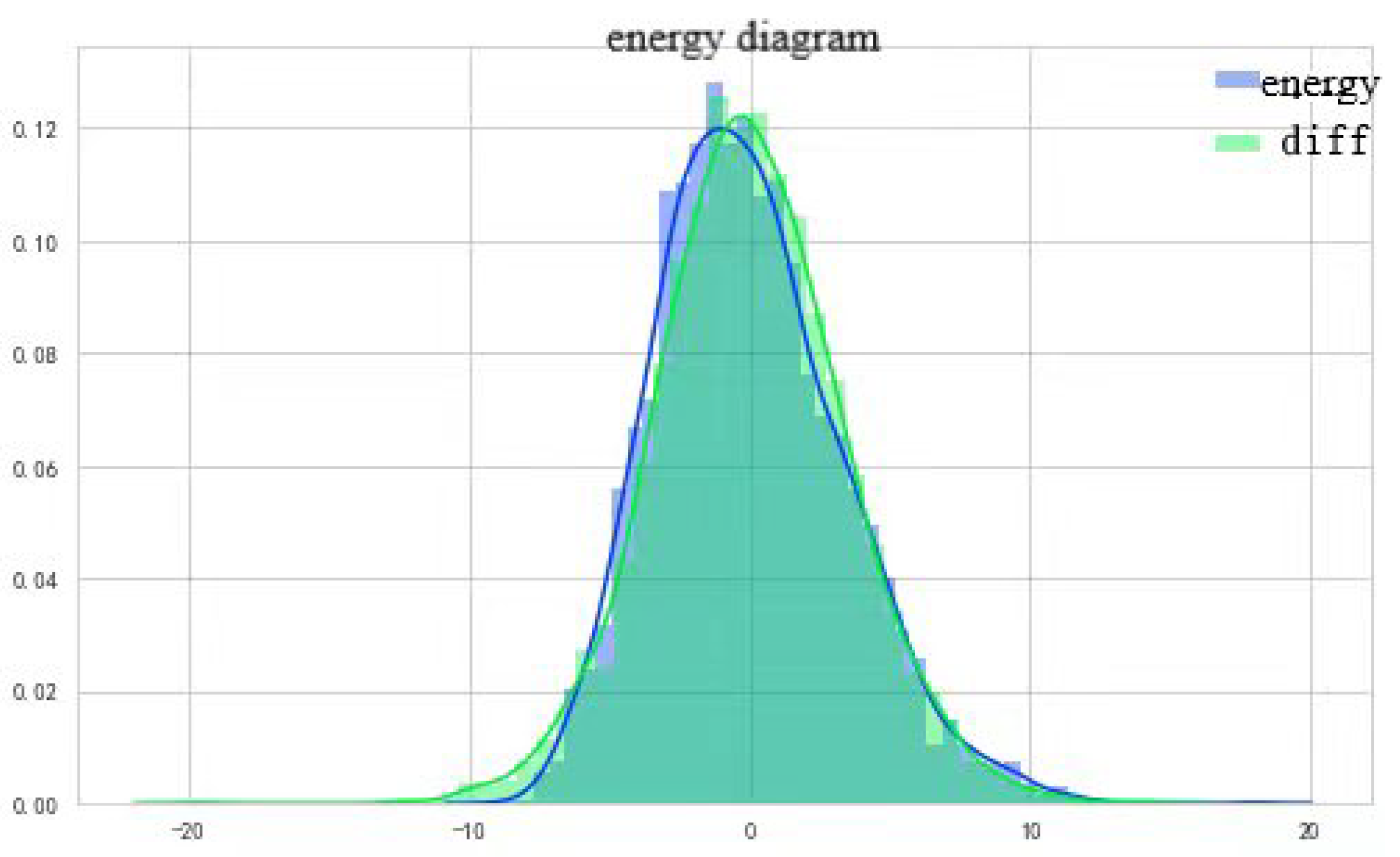
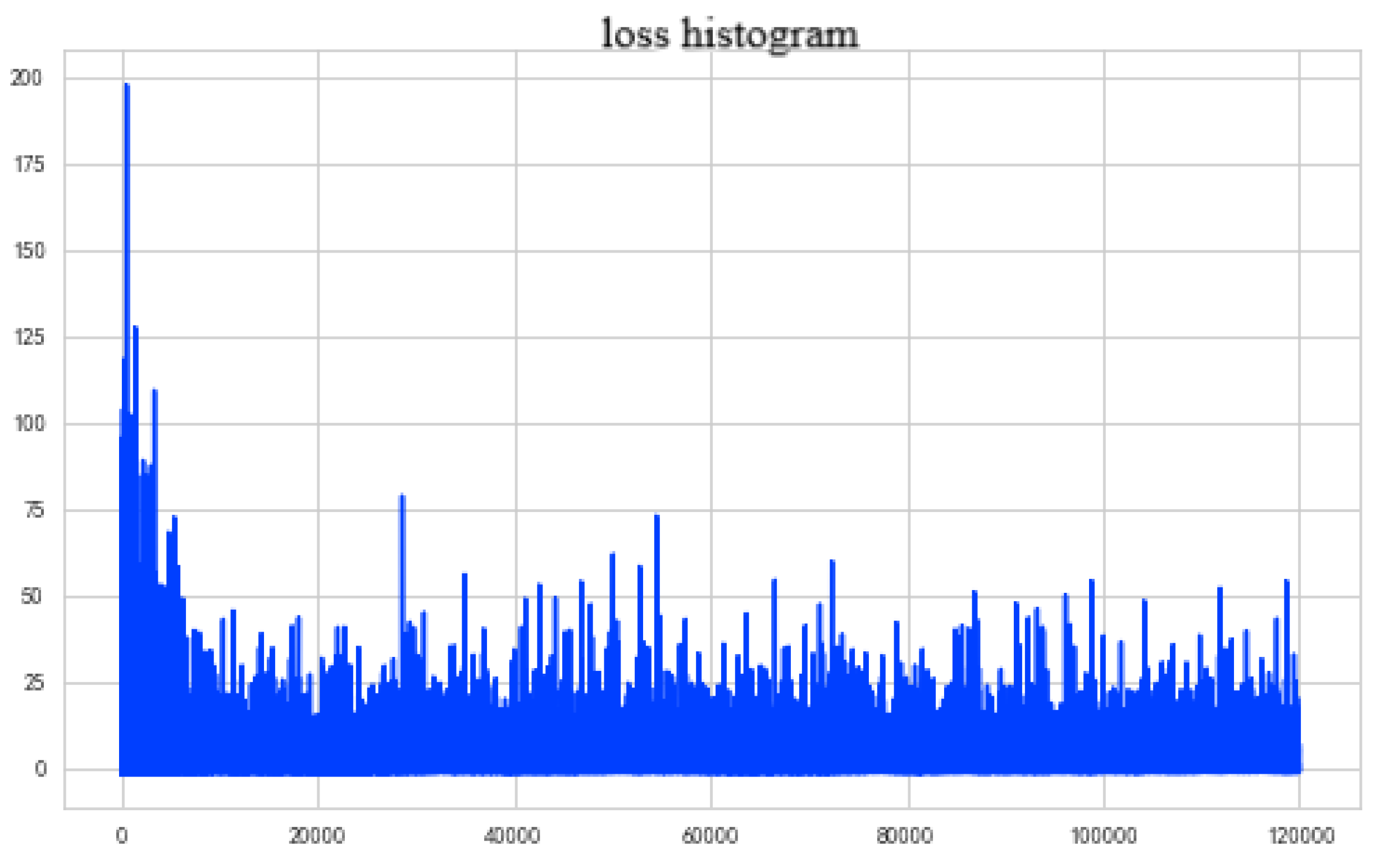
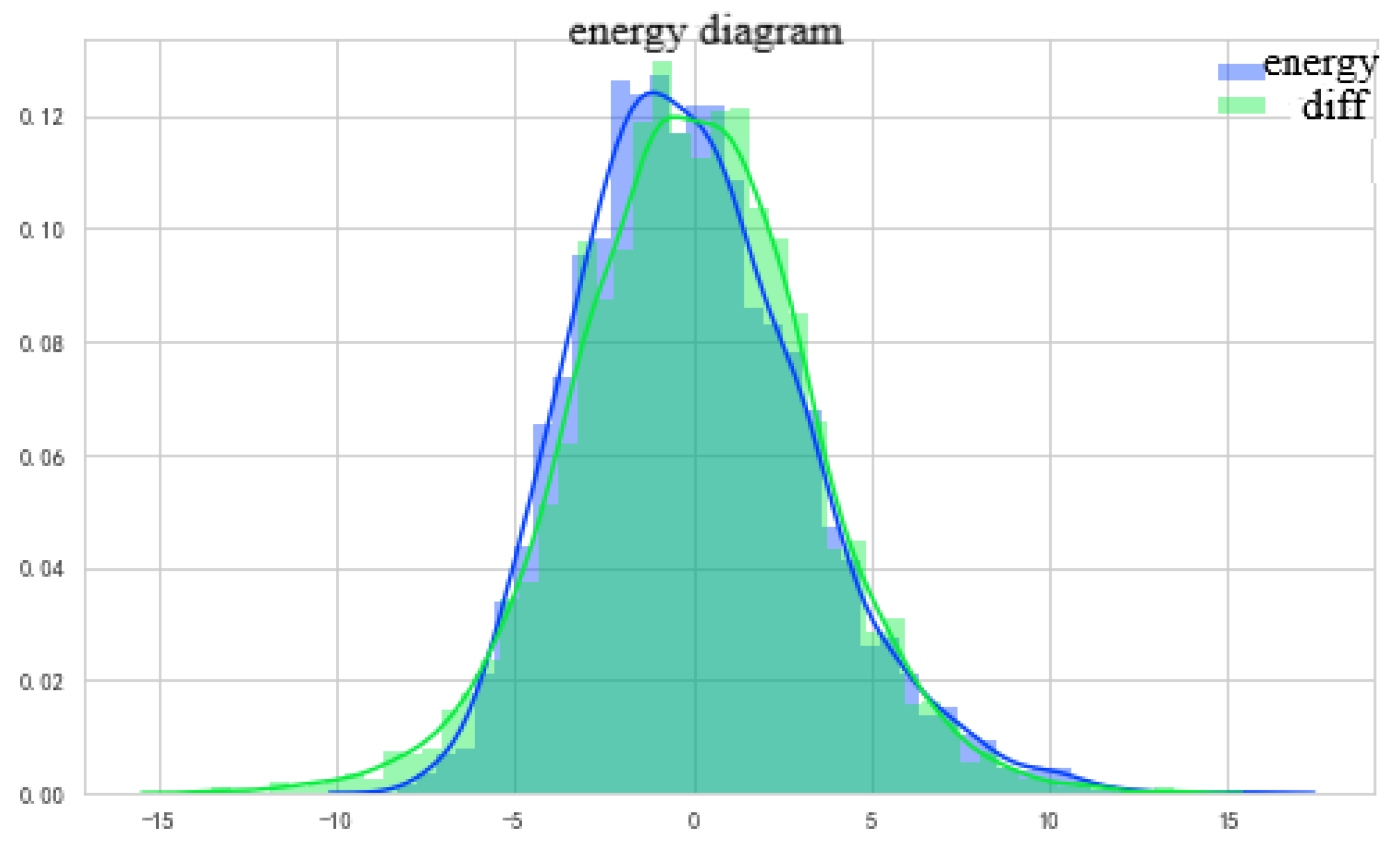
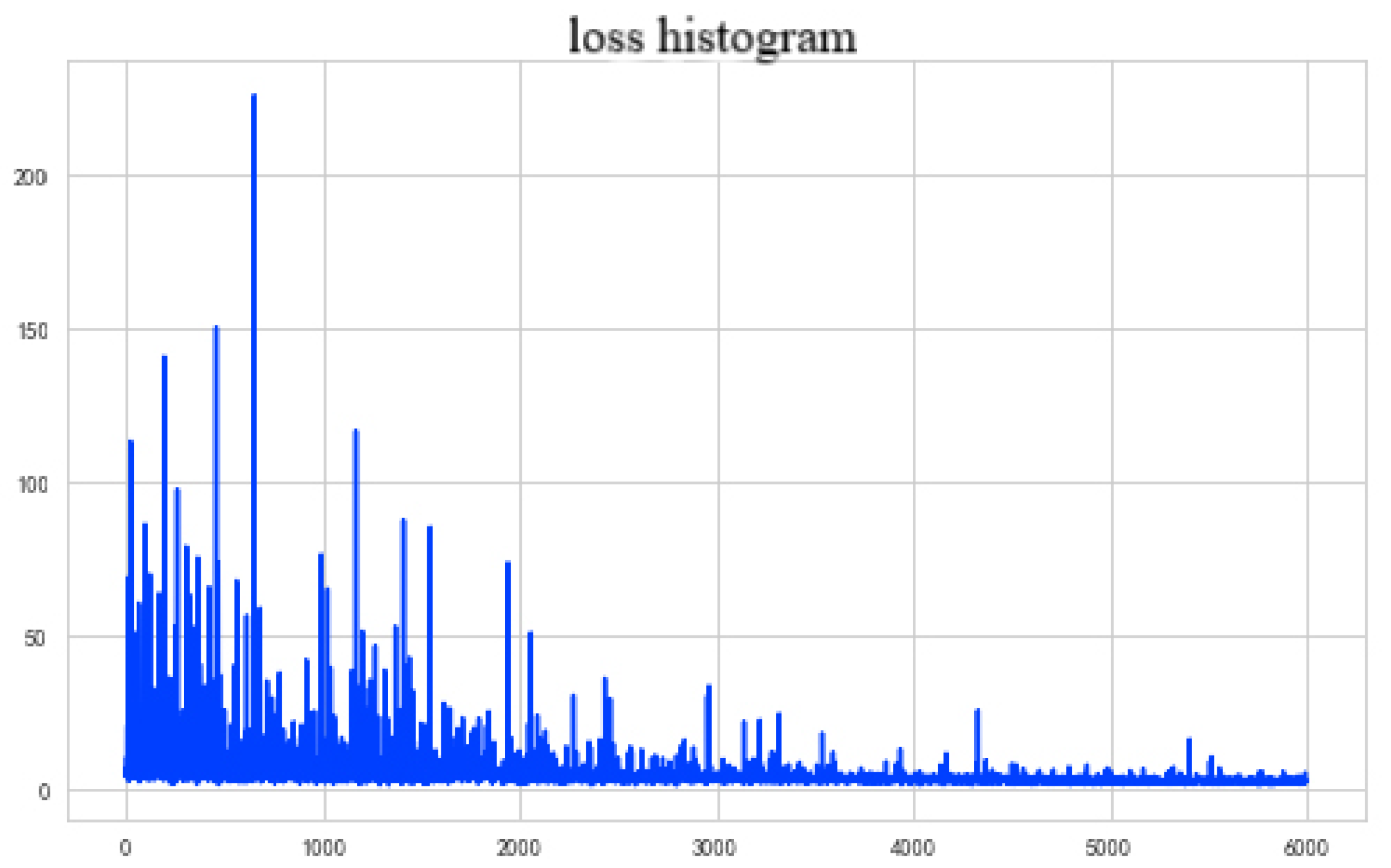
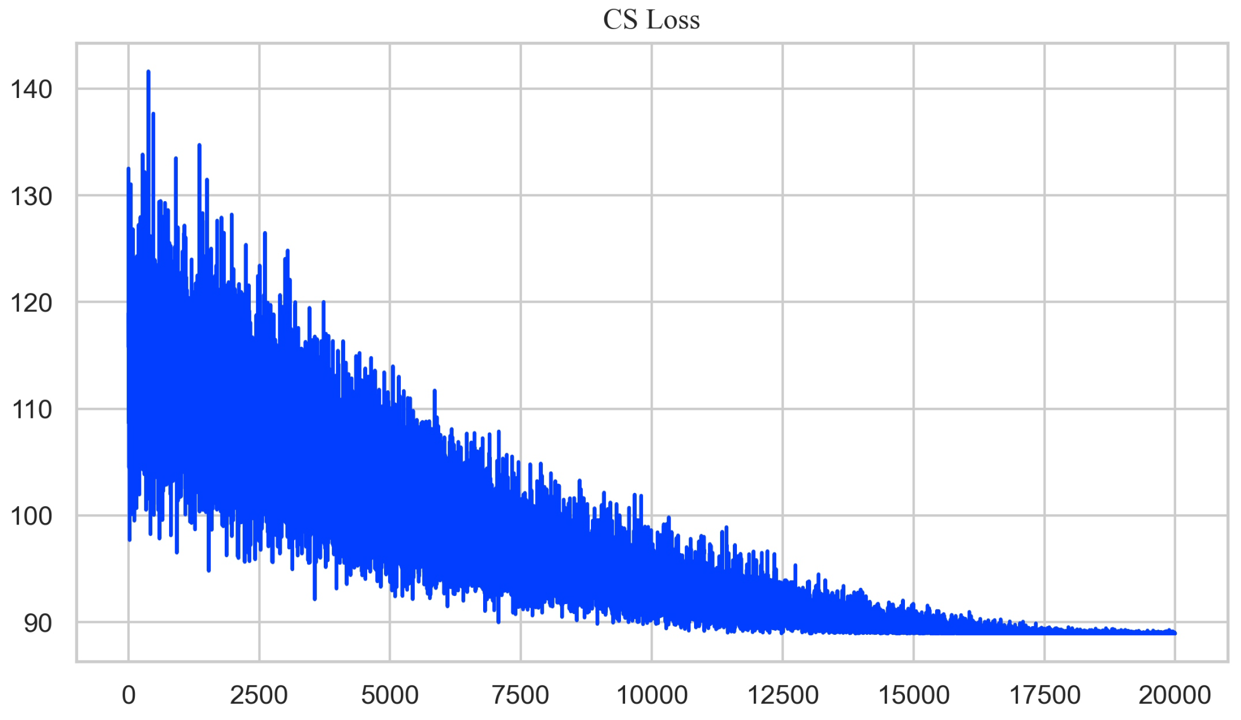
The negative ELBO loss histogram and energy graph estimated by the model with the CS structure are shown in Figure 5 and Figure 6, respectively, where the energy graph in Figure 6 was generated by the Python package PyMC3 (https://www.pymc.io/projects/docs/en/v3/pymc-examples/examples/getting_started.html) (accessed on 26 April 2023), which displays two simulated density curves: the blue one stands for the energy value at each MCMC sample point subtracted by the average energy (like conducting data centerization); the green one stands for the difference of the energy function (like deriving the derivative of a differential function). A normal energy distribution from an MCMC sampling indicates the sampling process tends to a stable point. It implies convergence of the MCMC sampling. More details on energy computation in MCMC sampling by PyMC3 can be found on this website (https://www.pymc.io/projects/docs/en/v3/api/inference.html#module-pymc3.sampling). Figure 5 and Figure 6 incorporate both popular methods for evaluating the convergence of the MCMC sampling in our Monte Carlo study. All energy graphs in the subsequent context have the same interpretation as they do here. We skip the tedious interpretations for all other energy graphs to save space.

Figure 5. Negative ELBO loss histogram: in Figure 5, the horizontal axis stands for the number of iterations in the MCMC sampling with size $n=100$, the vertical axis for the negative ELBO loss.

Figure 6. Energy graph: in Figure 6, the estimated distribution of energy is based on 1000 samples with size $n=100$.

As can be seen from Figure 5 and Figure 6, after several iterations of the MCMC algorithm, the negative ELBO loss is stable between 0 and 25, and the sample energy conversion distribution is basically consistent with the true energy distribution. Based on the sampling distribution and the trend graph, we can conclude that the MCMC algorithm is convergent.

For the case of the AR covariance structure, the prior distribution of each parameter in the model is specified as follows:

$$\begin{array}{cc}\hfill G_0=N& (0.4,10),\alpha =0.75,\hfill \\ \hfill b_i& \stackrel{iid}{\sim }N(0,0.01),\hfill \end{array}\begin{array}{cc}\hfill \mathit{\beta }& \sim N(0,10)\hfill \\ \hfill {\sigma }^2& \sim IG(1.25,0.01)\hfill \\ \hfill {\sigma }_s^2& \sim IG(3.76,9.566)\hfill \end{array}$$

(44)

Each parameter in the model is sampled and estimated using the MCMC method. The last 1000 iterations were taken to draw the posterior sampling trend diagram, as shown in Figure 7. Note that the DP-estimated density curves show different central locations from those in Figure 4, because they are generated from different prior distributions with different covariance structures (see the difference between Equations (43) and (44)).

Figure 7. Sampling results under the AR structure: The left panel gives the sampling distributions (smoothed by the kernel density estimation) for the parameters and the DP, which contain six pairs of DPs (each subject is observed $p=6$ variables in the simulation), each pair consisting of a DP generated from model (18) with the AR structure and a DP generated from the traditional model with the inverse-Wishart structure (sampling population specified by Equations (23), (24) and (44)). The orange line stands for sampling distribution under the SPAR model (18) and the blue line for the inverse-Wishart model; the right panel gives the the graphs of two Markov chains under the SPAR model (orange) and the inverse-Wishart model (blue), respectively, as well as the Markov chain for each individual DP (different color for each). Figure 4 and Figure 7 have the same structure in both axes for the two columns of graphs.

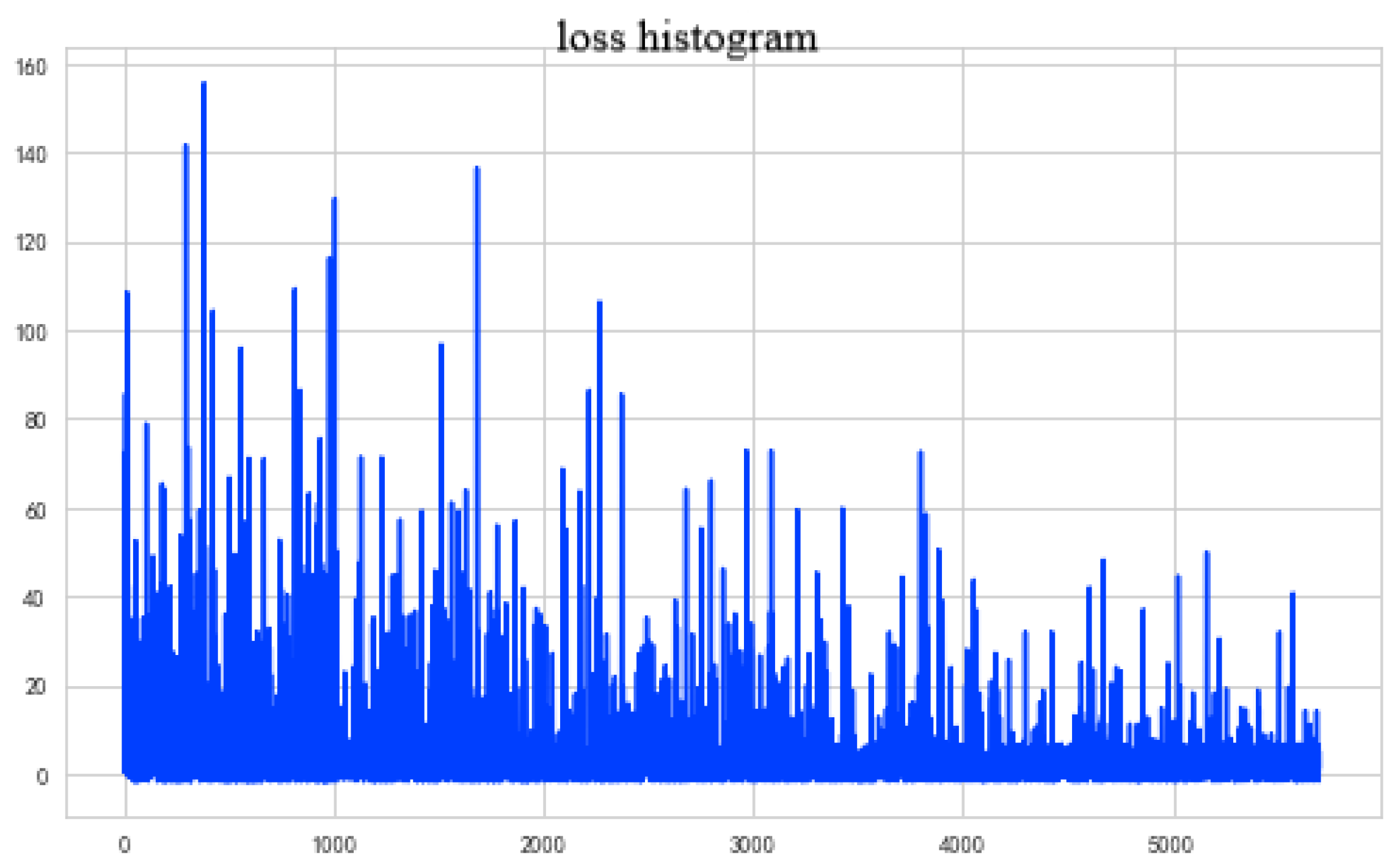
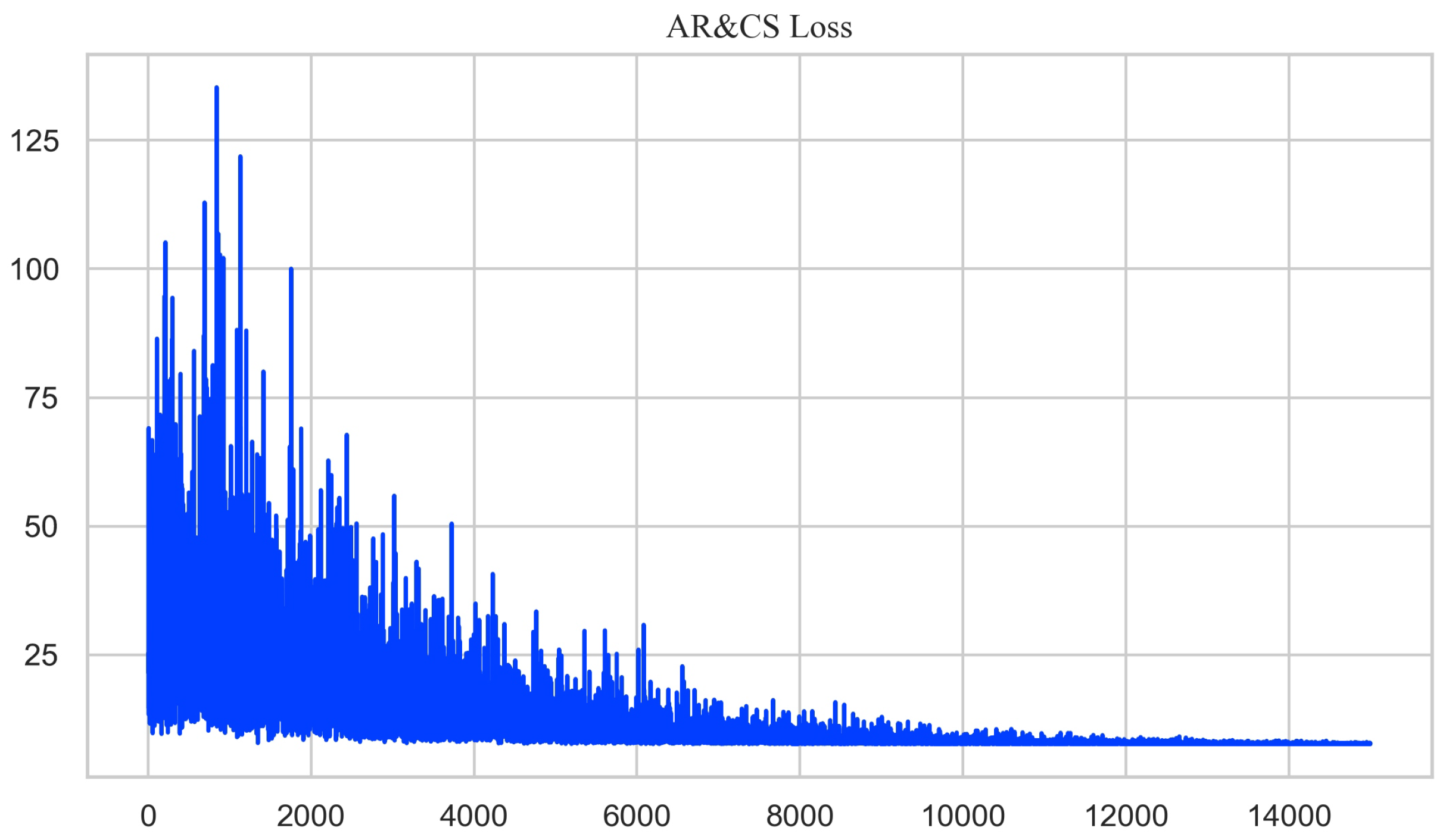
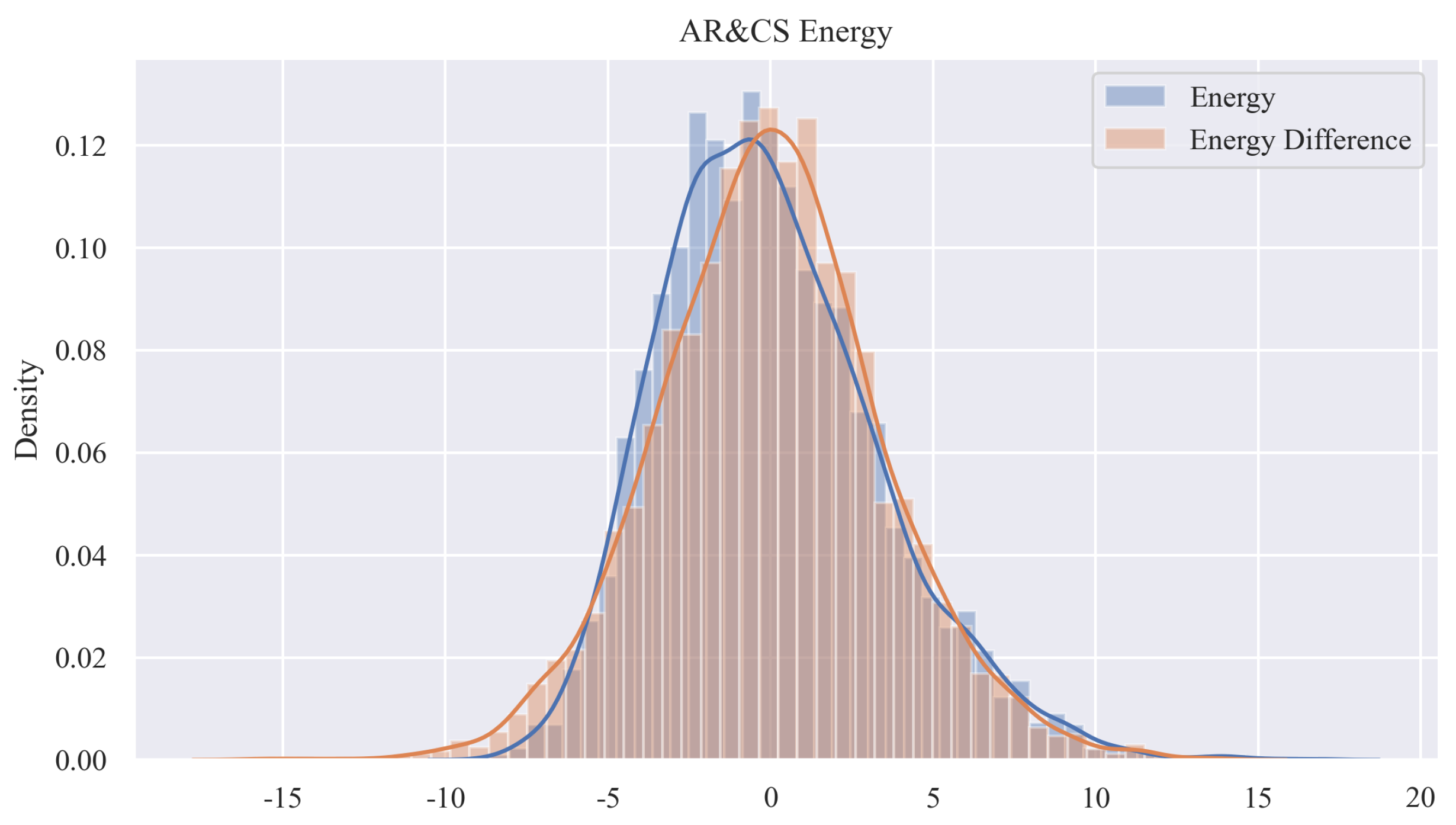
The histogram of negative ELBO loss and the energy graph for when the AR structure is estimated are shown in Figure 8 and Figure 9, respectively. They show that the histogram of the negative ELBO loss tends to be stable after several iterations, which is basically below 50, and the sample energy conversion distribution is basically consistent with the true energy distribution. Based on the posteriori sampling and the trend graph, it can be concluded that the algorithm converges quickly.

Figure 8. Negative ELBO loss histogram: in Figure 8, the horizontal axis stands for the number of iterations in the MCMC sampling with size $n=100$, the vertical axis for the negative ELBO loss.

Figure 9. Energy graph: In Figure 9, the estimated distribution of energy is based on 1000 samples with size $n=100$.

For the covariance of the mixed structure of CS and AR, the prior distribution of each parameter in the model is specified as follows:

$$\begin{array}{cc}\hfill G_0=N& (0.4,10),\alpha =0.75,\hfill \\ \hfill b_i& \stackrel{iid}{\sim }N(0,2.1),\hfill \end{array}\begin{array}{cc}\hfill \mathit{\beta }& \sim N(0,10),\hfill \\ \hfill {\sigma }^2& \sim IG(15.2,14),\hfill \\ \hfill {\sigma }_s^2& \sim IG(3.82,6.867).\hfill \end{array}$$

(45)

Each parameter in the model is sampled and estimated using the MCMC method. The last 1000 iterations were taken to draw the posterior sampling trend graph, as shown in Figure 10. The negative ELBO loss histogram and the model energy graph are shown in Figure 11 and Figure 12, respectively.

Figure 10. Sampling results under the mixed structure of CS and AR: The left panel gives the sampling distributions (smoothed by the kernel density estimation) for the parameters and the DP, which contain six pairs of DPs (each subject is observed $p=6$ variables in the simulation), each pair consisting of a DP generated from model (18) with the mixed structure of CS and AR and a DP generated from the traditional model with the inverse-Wishart structure (sampling population specified by Equations (23), (24) and (45)). The orange line stands for sampling distribution under the SPAR model (18) and the blue line for the inverse-Wishart model; the right panel gives the the graphs of two Markov chains under the SPAR model (orange) and the inverse-Wishart model (blue), respectively, as well as the Markov chain for each individual DP (different color for each). Figure 4 and Figure 10 have the same structure in both axes for the two columns of graphs.

Figure 11. Negative ELBO loss histogram: in Figure 11, the horizontal axis stands for the number of iterations in the MCMC sampling with size $n=100$, the vertical axis for the negative ELBO loss.

Figure 12. Energy graph: in Figure 12, the estimated distribution of energy is based on 1000 samples with size $n=100$.

As can be seen from the histogram of the negative ELBO loss in Figure 11, the negative ELBO loss is basically under control between 0 and 30, after several iterations of the algorithm, and the sample energy conversion distribution is basically consistent with the true energy distribution. Based on the posteriori sampling and the trend graph, we can conclude that the algorithm is convergent.

For the case of independent structure covariance, the prior distributions of the parameters in the model are specified as follows:

$$\begin{array}{cc}\hfill G_0=N& (0.672,10),\alpha =0.75,\hfill \\ \hfill b_i& \stackrel{iid}{\sim }N(0,1.106),\hfill \end{array}\begin{array}{cc}\hfill \mathit{\beta }& \sim N(0,20),\hfill \\ \hfill {\sigma }^2& \sim IG(2.22,7.48),\hfill \\ \hfill {\sigma }_s^2& \sim IG(3.20,3.443).\hfill \end{array}$$

(46)

The MCMC method was used to sample and estimate each parameter in the model. The last 1000 iterations were taken to draw the posterior sampling trend graph shown in Figure 13.

Figure 13. Sampling results under the independent structure: The left panel gives the sampling distributions (smoothed by the kernel density estimation) for the parameters and the DP, which contain six pairs of DPs (each subject is observed $p=6$ variables in the simulation), each pair consisting of a DP generated from model (18) with the independent structure and a DP generated from the traditional model with the inverse-Wishart structure (sampling population specified by Equations (23), (24) and (46)). The orange line stands for sampling distribution under the SPAR model (18) and the blue line for the inverse-Wishart model; the right panel gives the the graphs of two Markov chains under the SPAR model (orange) and the inverse-Wishart model (blue), respectively, as well as the Markov chain for each individual DP (different color for each). Figure 4 and Figure 13 have the same structure in both axes for the two columns of graphs.

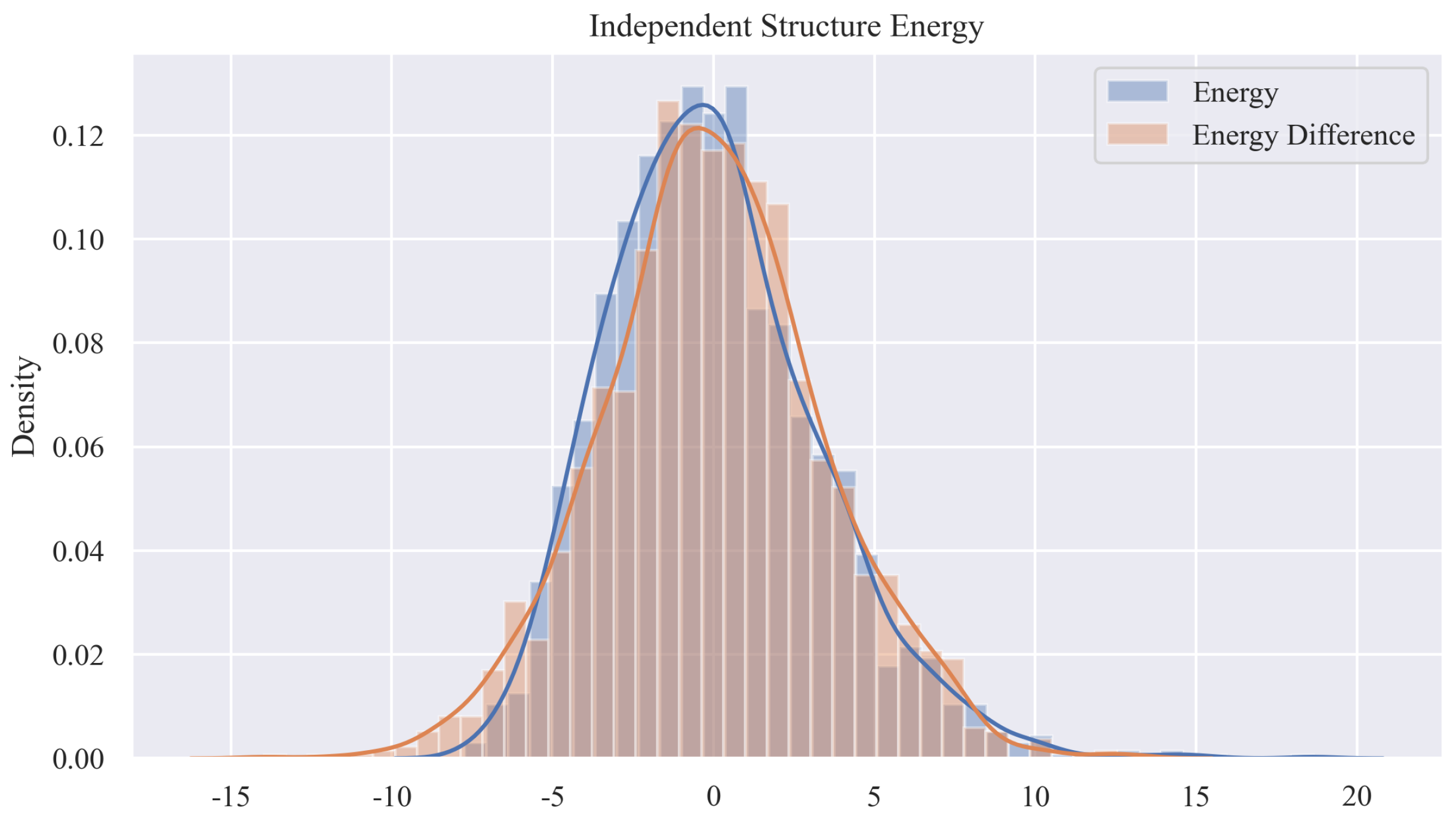
The negative ELBO loss histogram and the model energy graph are shown in Figure 14 and Figure 15, respectively. It can be seen that the negative ELBO loss approaches 0 quickly. Based on the posterior sampling and the trend diagram, we can conclude that the algorithm is convergent.

Figure 14. Negative ELBO loss histogram: in Figure 14, the horizontal axis stands for the number of iterations in the MCMC sampling with size $n=100$, the vertical axis for the negative ELBO loss.

Figure 15. Energy graph: in Figure 15, the estimated distribution of energy is based on 1000 samples with size $n=100$.

The above model is applied to the estimation of covariance matrices, correlation matrices, and model errors. We compare it with with the inverse-Wishart method. The outcomes of the estimation errors are shown in Table 2:

Table 2. Estimated RMSE, $L_1$, and $L_2$ based on covariance matrix $\mathbf{\Sigma }$.

Loss Function	Model	C1	C2	C3	C4
RMSE	SPAR	0.9960	0.1037	0.8995	1.5358
	Inv-W	2.9691	2.9352	3.4804	3.3285
$L_1$	SPAR	0.1810	0.1201	1.3217	0.9558
	Inv-W	1.8389	1.4632	3.0516	1.2926
$L_2$	SPAR	0.1289	0.1345	1.7575	0.6044
	Inv-W	0.2405	0.9576	2.8083	1.7565

C1 represents the covariance of the complex symmetry (CS) structure; C2 represents the AR structure covariance; C3 represents the mixed structure covariance of CS and AR; C4 represents independent structure covariance; and Inv-W = inverse-Wishart.

Similarly, the estimation results of the four corresponding correlation matrices are shown in Table 3:

Table 3. Estimated RMSE, $L_1$, and $L_2$ based on correlation matrix $\mathit{R}$.

Loss Function	Model	C1	C2	C3	C4
RMSE	SPAR	0.1628	1.1417	0.3775	0.1542
	Inv-W	0.2308	2.4152	0.9115	0.2771
$L_1$	SPAR	0.0956	0.5482	0.0631	1.2354
	Inv-W	0.1519	1.1424	0.1756	1.9137
$L_2$	SPAR	0.1013	0.9809	0.4937	0.5854
	Inv-W	0.1238	1.1935	0.5205	0.6484

C1 represents the covariance of the complex symmetry (CS) structure; C2 represents the AR structure covariance; C3 represents the mixed structure covariance of CS and AR; and C4 represents independent structure covariance.

In Table 2 and Table 3, the covariance models are compared with each other based on three types of loss functions. In estimating the four covariance structures, the SPAR model performs better than the traditional inverse-Wishart method for each covariance structure. The estimation error of the SPAR model is much smaller than that of the inverse-Wishart method. When estimating the correlation matrix, except for the relatively poor SPAR performance under the strict AR structure, all other models perform roughly the same based on the quadratic loss function $L_2(\widehat{\mathbf{\Sigma }},\mathbf{\Sigma })$. Based on the comparison of the estimation errors in Table 2 and Table 3, the SPAR model shows fairly good performance in estimating the covariance matrix and correlation matrix.

7.3. Analysis of a Real Wind Speed Dataset

To verify the effectiveness of the SPAR model built in this paper in practical application, we employ the Hongming data, which contain the ground meteorological data of Dingxin Station, Jinta County, Jiuquan City, Gansu Province, China. We use the SPAR model and the MCMC method to estimate the covariance matrix and correlation matrix under four different covariance structures (CS, AR, the mixture of CS and AR, and unstructured) and compare the estimates with those from the traditional Bayesian estimation by the inverse-Wishart method. The covariance structure of the four cases is shown in Equation (41), and the mean square error is shown in Equation (42). The real data are arranged into a longitudinal data structure, as shown in Table 1 with $n=100$, $p=6$, and $k=1$. The following graphs are plotted in the same way as in the corresponding graphs in the Monte Carlo study in Section 7.2 but with real data input in the same Python program.

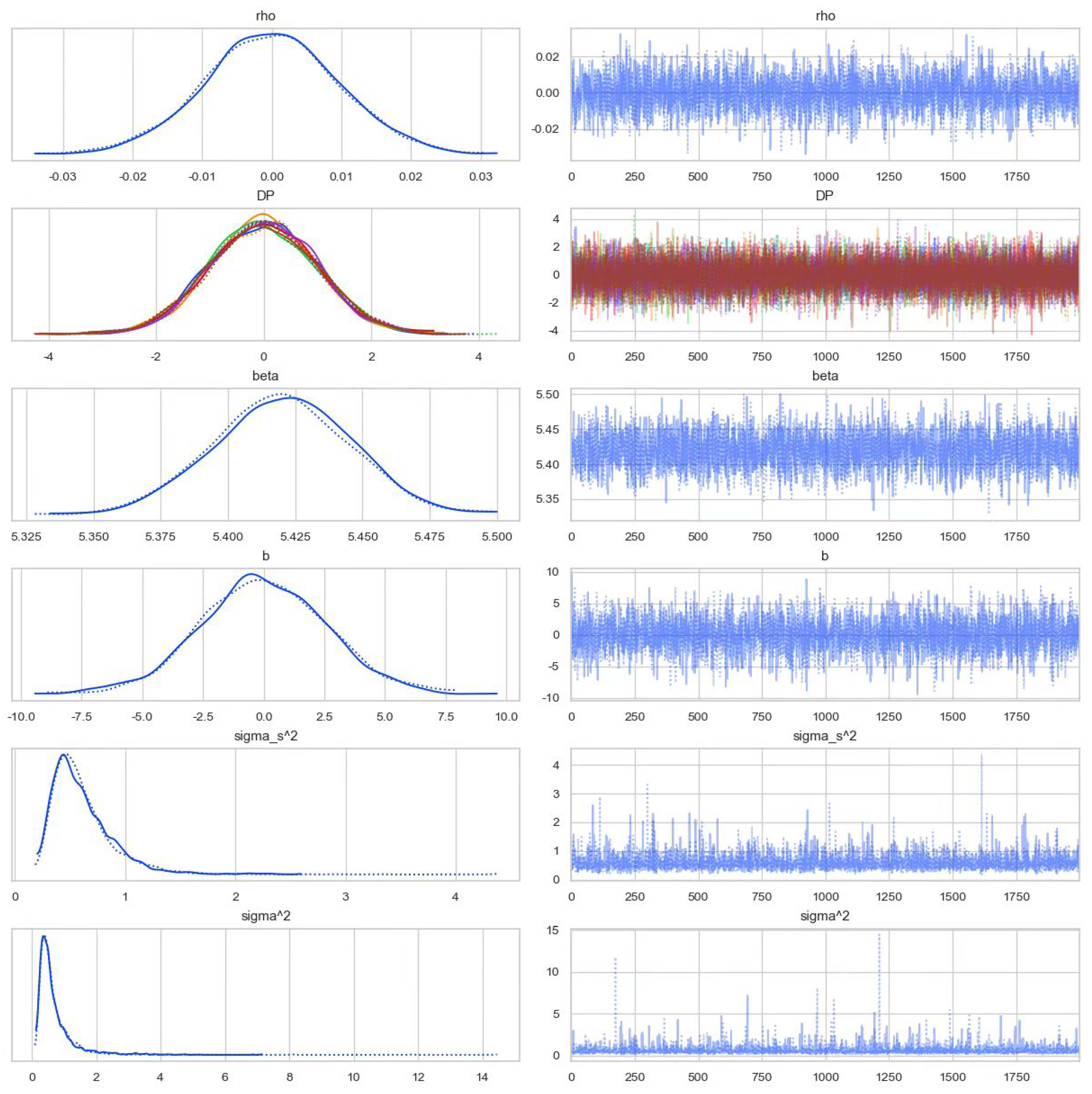
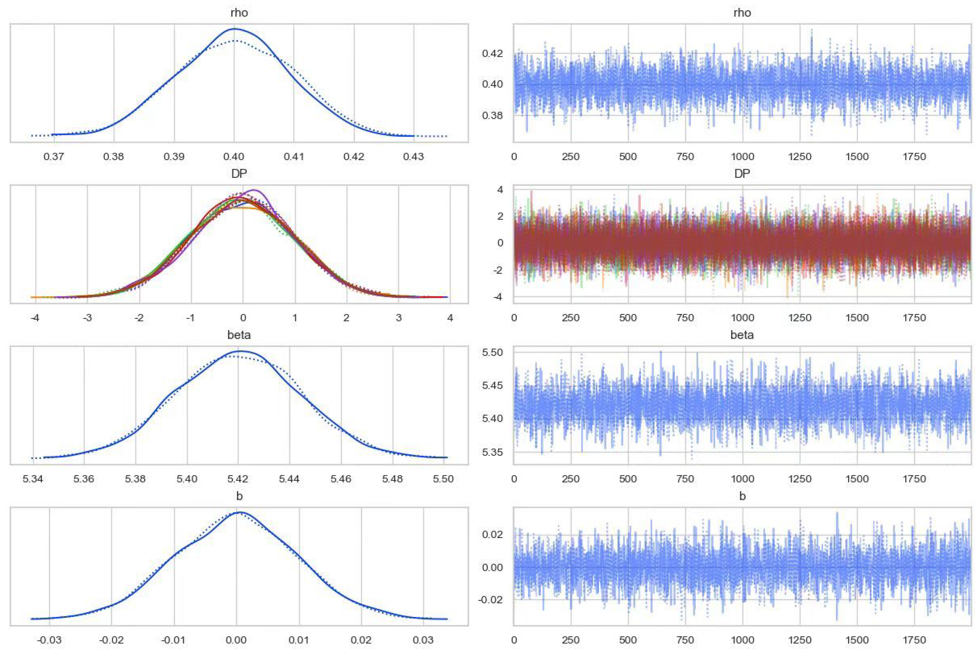
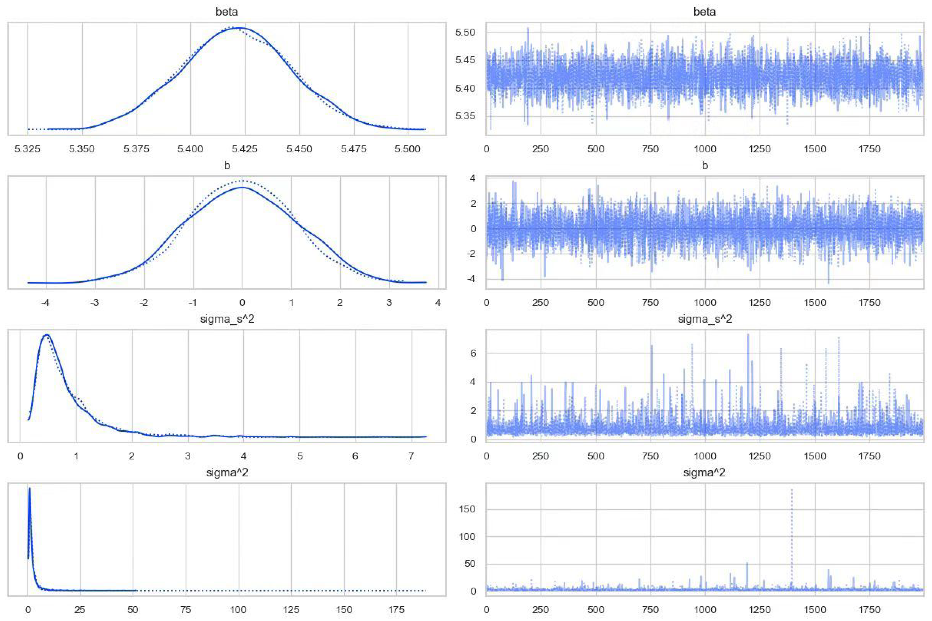
For the case of CS covariance structure, each parameter in the model is sampled and estimated using the MCMC method. The last 1000 iterations are taken to draw the posterior sampling trend diagram, as shown in Figure 16.

Figure 16. Sampling results under the CS structure: The left panel gives the sampling distributions (smoothed by the kernel density estimation) for the parameters and the DP, which contain six pairs of DPs (each subject is observed $p=6$ variables in the simulation), each pair consisting of a DP generated from model (18) with the CS structure and a DP generated from the traditional model with the inverse-Wishart structure (sampling population specified by Equations (23), (24) and (43)). The real blue line stands for sampling distribution under the SPAR model (18) and the dotted blue line for the inverse-Wishart model; the right panel gives the the graphs of two Markov chains under the SPAR model (real line) and the inverse-Wishart model (dotted line), respectively, as well as the Markov chain for each individual DP (different color for each). Figure 4 and Figure 16 have the same structure in both axes for the two columns of graphs.

The negative ELBO loss histogram and the model energy graph are shown in Figure 17 and Figure 18, respectively. It can be seen that the negative ELBO loss approaches 0 quickly, and the sample energy conversion distribution is basically consistent with the true energy distribution. Based on the posterior sampling and the trend diagram, we can conclude that the algorithm is convergent.

Figure 17. Negative ELBO loss histogram: in Figure 17, the horizontal axis stands for the number of iterations in the MCMC algorithm with size $n=100$, the vertical axis for the negative ELBO loss.

Figure 18. Energy graph: In Figure 18, the estimated distribution of energy is based on 1000 samples with size $n=100$.

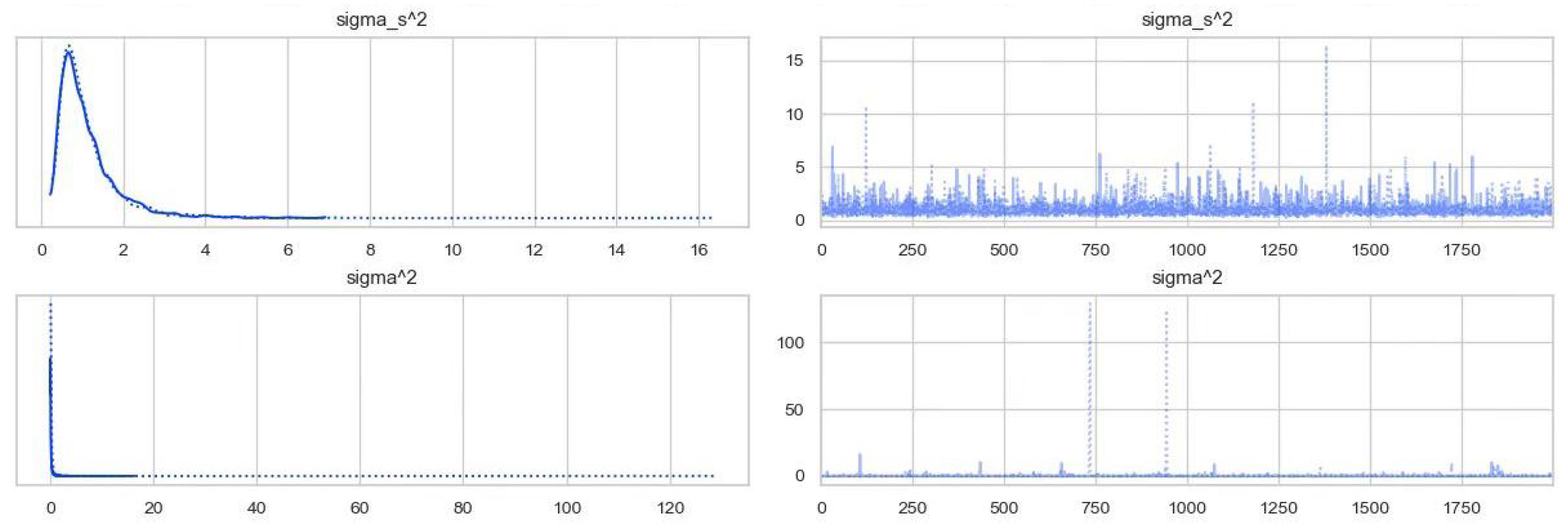
For the case of the AR covariance structure, each parameter in the model is sampled and estimated using the MCMC method. The last 1000 iterations are taken to draw the posterior sampling trend diagram, as shown in Figure 19:

Figure 19. Sampling results under the AR structure: The left panel gives the sampling distributions (smoothed by the kernel density estimation) for the parameters and the DP, which contain six pairs of DPs (each subject is observed $p=6$ variables in the simulation), each pair consisting of a DP generated from model (18) with the AR structure and a DP generated from the traditional model with the inverse-Wishart structure (sampling population specified by Equations (23), (24) and (44)). The real blue line stands for sampling distribution under the SPAR model (18) and the dotted blue line for the inverse-Wishart model; the right panel gives the the graphs of two Markov chains under the SPAR model (real line) and the inverse-Wishart model (dotted line), respectively, as well as the Markov chain for each individual DP (different color for each). Figure 4 and Figure 19 have the same structure in both axes for the two columns of graphs.

The negative ELBO loss histogram and the energy graph estimated by the model under the AR structure are shown in Figure 20 and Figure 21, respectively. It shows that the histogram of the negative ELBO loss approaches 0 quickly. Based on the posteriori sampling and the trend graph, it can be concluded that the algorithm converges quickly.

Figure 20. Negative ELBO loss histogram: in Figure 20, the horizontal axis stands for the number of iterations in the MCMC algorithm with size $n=100$, the vertical axis for the negative ELBO loss.

Figure 21. Energy graph: in Figure 21, the estimated distribution of energy is based on 1000 samples with size $n=100$.

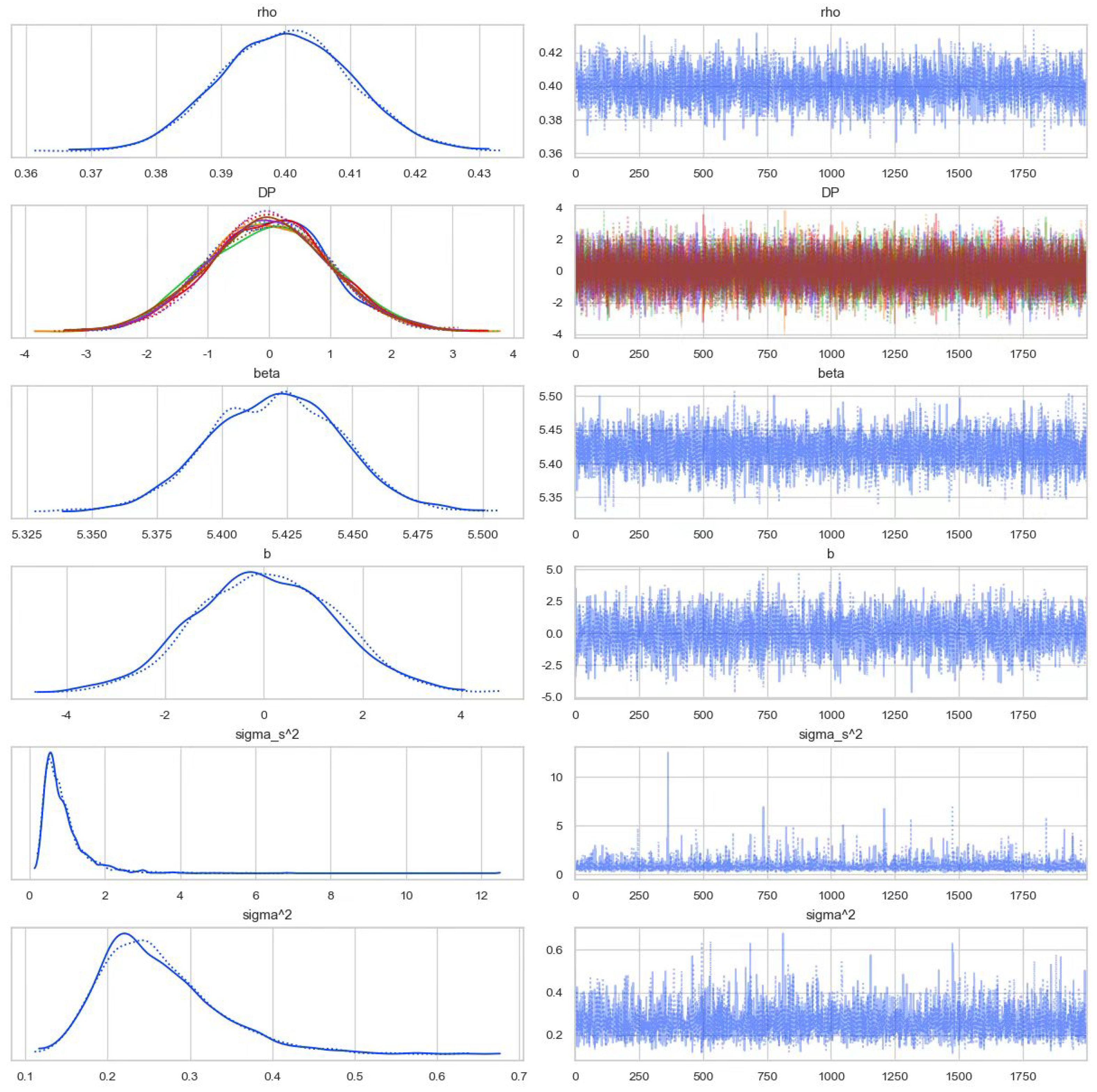
For the covariance of the mixed structure of CS and AR, each parameter in the model is sampled and estimated using the MCMC method. The last 1000 iterations are taken to draw the posterior sampling trend graph, as shown in Figure 22. The negative ELBO loss histogram and the model energy graph are shown in Figure 23 and Figure 24, respectively.

Figure 22. Sampling results under the mixed structure of CS and AR: The left panel gives the sampling distributions (smoothed by the kernel density estimation) for the parameters and the DP, which contain six pairs of DPs (each subject is observed $p=6$ variables in the simulation), each pair consisting of a DP generated from model (18) with the mixed structure of CS and AR and a DP generated from the traditional model with the inverse-Wishart structure (sampling population specified by Equations (23), (24) and (45)). The real blue line stands for sampling distribution under the SPAR model (18) and the dotted blue line for the inverse-Wishart model; the right panel gives the the graphs of two Markov chains under the SPAR model (real line) and the inverse-Wishart model (dotted line), respectively, as well as the Markov chain for each individual DP (different color for each). Figure 4 and Figure 22 have the same structure in both axes for the two columns of graphs.

Figure 23. Negative ELBO loss histogram: in Figure 23,the horizontal axis stands for the number of iterations in the MCMC algorithm with size $n=100$, the vertical axis for the negative ELBO loss.

Figure 24. Energy graph: in Figure 24, the estimated distribution of energy is based on 1000 samples with size $n=100$.

As can be seen from the histogram of the negative ELBO loss in Figure 23, the negative ELBO loss approaches 0 quickly after several iterations of the algorithm. Based on the posteriori sampling and the trend graph, we can conclude that the algorithm is convergent.

For the case of independent structure covariance, the MCMC method is used to sample and estimate each parameter in the model. The last 1000 iterations are taken to draw the posterior sampling trend graph shown in Figure 25.

Figure 25. Sampling results under an independent structure: The left panel gives the sampling distributions (smoothed by the kernel density estimation) for the parameters and the DP, which contain six pairs of DPs (each subject is observed $p=6$ variables in the simulation), each pair consisting of a DP generated from model (18) with the independent structure and a DP generated from the traditional model with the inverse-Wishart structure (sampling population specified by Equations (23), (24) and (46)). The real blue line stands for sampling distribution under the SPAR model (18) and the dotted blue line for the inverse-Wishart model; the right panel gives the the graphs of two Markov chains under the SPAR model (real line) and the inverse-Wishart model (dotted line), respectively, as well as the Markov chain for each individual DP (different color for each). Figure 4 and Figure 25 have the same structure in both axes for the two columns of graphs.

The negative ELBO loss histogram and the model energy graph are shown in Figure 26 and Figure 27, respectively. It can be seen that the negative ELBO loss approaches 0 quickly. Based on the posterior sampling and trend diagram, we can conclude that the algorithm is convergent.

Figure 26. Negative ELBO loss histogram: in Figure 26, the horizontal axis stands for the number of iterations in the MCMC algorithm with size $n=100$, the vertical axis for the negative ELBO loss.

Figure 27. Energy graph: in Figure 27, the estimated distribution of energy is based on 1000 samples with size $n=100$.

In Table 4 and Table 5, the covariance models are compared with each other based on three types of loss functions, RMSE, $L_1$, and $L_2$. When using the four covariance structures based on either the covariance matrix or the correlation matrix, the SPAR model always performs better than the traditional inverse-Wishart method—it always has a smaller value of RMSE, $L_1$, or $L_2$ when comparing the SPAR model with the Inv-W model under the same covariance structure C1, C2, C3, or C4 in Table 4 and Table 5.

Table 4. Estimated RMSE, $L_1$, and $L_2$ based on covariance matrix $\mathbf{\Sigma }$.

Loss Function	Model	C1	C2	C3	C4
RMSE	SPAR	0.0831	0.0962	0.08837	0.0981
	Inv-W	0.4120	0.6826	0.3181	0.4064
$L_1$	SPAR	0.1360	0.1996	0.1465	0.2508
	Inv-W	46.6743	16.8967	19.0260	14.3543
$L_2$	SPAR	0.0870	0.0826	0.2084	0.3517
	Inv-W	661.4643	142.3157	450.6686	340.6994

C1 represents the covariance of the complex symmetry (CS) structure; C2 represents the AR structure covariance; C3 represents the mixed structure covariance of CS and AR; C4 represents independent structure covariance; and Inv-W = inverse-Wishart.

Table 5. Estimated RMSE, $L_1$, and $L_2$ based on correlation matrix $\mathit{R}$.

Loss Function	Model	C1	C2	C3	C4
RMSE	SPAR	0.0187	0.5359	0.1976	0.1985
	Inv-W	0.6585	0.6486	0.6515	0.7580
$L_1$	SPAR	0.0066	0.1670	0.0662	0.1846
	Inv-W	0.0968	4.8245	0.3174	0.8035
$L_2$	SPAR	0.0036	0.0132	0.0080	0.0939
	Inv-W	0.0079	1.3683	0.1202	0.3488

C1 represents the covariance of the complex symmetry (CS) structure; C2 represents the AR structure covariance; C3 represents the mixed structure covariance of CS and AR; and C4 represents independent structure covariance.

8. Concluding Remarks

The SPAR model (18) provides an explicitly complete semiparametric solution to the estimation of model parameters through the MCMC algorithm. Compared with the model formulation in Quintana et al. [4], the MCMC algorithm for posterior inference on model (18) is easier to implement and may converge faster because of the explicit simple posterior distributions of the model parameters. An effective and fast-converging MCMC algorithm plays an important role in Bayesian statistical inference. The SPAR model (18) gains some trade-off in easy implementation and fast convergence in the MCMC algorithm by imposing simpler assumptions on model parameters.

With regard to the option of choosing the initial values for estimating model parameters by the MCMC algorithm, we recommend using a numerical optimization method such as the maximum posteriori (MAP) estimation to obtain an estimator as the initial value of a parameter. It is likely to speed up the convergence speed of the sampling parameter. We employ the Gibbs sampling algorithm when estimating the parameters in the model. The convergence diagnosis of Markov chains generated by the MCMC algorithm is assessed by the posterior sampling trend plot, negative ELBO histogram, and the energy graph, which show the observation of fast convergence of the MCMC sampling process. By applying the SPAR model to four different covariance structures through both Monte Carlo study and a real dataset, we illustrate its effectiveness in handling nonstationary forms of covariance structures and its domination over the traditional inverse-Wishart method.

It should be pointed out that the effectiveness and fast convergence of the MCMC algorithm depend on both model assumption and the priors of model parameters. Our Monte Carlo study was carried out by choosing normal priors for the model parameters and the inverse Gamma distribution for the variance components. This choice led to the easy implementation of the MCMC algorithm. It will be an interesting future research direction to develop some meaningful criteria for model and algorithm comparison in the area of Bayesian nonparametric longitudinal data analysis. The main purpose of our paper is to give an easily implementable approach to this area with a practical illustration. We can conclude that the complete semiparametric approach to Bayesian longitudinal data analysis in this paper is a significant complement to the area studied by some influential peers, such as Mukhopadhyay and Gelfand (1997, [21]), Quintana et al. (2016, [4]), and others.

References

- Pullenayegum, E.M.; Lim, L.S. Longitudinal data subject to irregular observation: A review of methods with a focus on visit processes, assumptions, and study design. Statist. Methods Med. Res. 2016, 25, 2992–3014. [Google Scholar] [CrossRef] [PubMed]
- Chakraborty, R.; Banerjee, M.; Vemuri, B.C. Statistics on the space of trajectories for longitudinal data analysis. In Proceedings of the 2017 IEEE 14th International Symposium on Biomedical Imaging (ISBI 2017), Melbourne, VIC, Australia, 18–21 April 2017; pp. 999–1002. [Google Scholar]
- Xiang, D.; Qiu, P.; Pu, X. Nonparametric regession analysis of multivariate longitudinal data. Stat. Sin. 2013, 23, 769–789. [Google Scholar]
- Quintana, F.A.; Johnson, W.O.; Waetjen, L.E.; BGold, E. Bayesian nonparametric longitudinal data analysis. J. Am. Statist. Assoc. 2016, 111, 1168–1181. [Google Scholar] [CrossRef]
- Cheng, L.; Ramchandran, S.; Vatanen, T.; Lietzén, N.; Lahesmaa, R.; Vehtari, A.; Lähdesmäki, H. An additive Gaussian process regression model for interpretable non-parametric analysis of longitudinal data. Nat. Commun. 2019, 10, 1798. [Google Scholar] [CrossRef]
- Kleinman, K.P.; Ibrahim, J.G. A semiparametric Bayesian approach to the random effects model. Biometrics 1998, 54, 921–938. [Google Scholar] [CrossRef] [PubMed]
- Gao, F.; Zeng, D.; Couper, D.; Lin, D.Y. Semiparametric regression analysis of multiple right- and interval-censored events. J. Am. Statist. Assoc. 2019, 114, 1232–1240. [Google Scholar] [CrossRef] [PubMed]
- Lee, Y. Semiparametric regression. J. Am. Statist. Assoc. 2006, 101, 1722–1723. [Google Scholar] [CrossRef]
- Sun, Y.; Sun, L.; Zhou, J. Profile local linear estimation of generalized semiparametric regression model for longitudinal data. Lifetime Data Anal. 2013, 19, 317–349. [Google Scholar] [CrossRef] [PubMed]
- Zeger, S.L.; Diggle, P.J. Semiparametric models for longitudinal data with application to CD4 cell numbers in HIV seroconverters. Biometrics 1994, 50, 689–699. [Google Scholar] [CrossRef] [PubMed]
- Li, Y.; Lin, X.; Müller, P. Bayesian inference in semiparametric mixed models for longitudinal data. Biometrics 2010, 66, 70–78. [Google Scholar] [CrossRef] [PubMed]
- Hunag, Y.X. Quantile regression-based Bayesian semiparametric mixed-effects models for longitudinal data with non-normal, missing and mismeasured covariate. J. Statist. Comput. Simul. 2016, 86, 1183–1202. [Google Scholar] [CrossRef]
- Li, J.; Zhou, J.; Zhang, B.; Li, X.R. Estimation of high dimensional covariance matrices by shrinkage algorithms. In Proceedings of the 2017 20th International Conference on Information Fusion (Fusion), Xi’an, China, 10–13 July 2017; pp. 955–962. [Google Scholar]
- Doss, H.; Park, Y. An MCMC approach to empirical Bayes inference and Bayesian sensitivity analysis via empirical processes. Ann. Statist. 2018, 46, 1630–1663. [Google Scholar] [CrossRef]
- Neal, R.M. Markov chain sampling methods for Dirichlet process mixture models. J. Comput. Graph. Statist. 2000, 9, 249–265. [Google Scholar]
- Kingma, D.P.; Welling, M. Auto-encoding variational Bayes. In Proceedings of the International Conference on Learning Representations (ICLR), Banff, AB, Canada, 14–16 April 2014. [Google Scholar]
- Csiszar, I. I-Divergence geometry of probability distributions and minimization problems. Ann. Probab. 1975, 3, 146–158. [Google Scholar] [CrossRef]
- Rasmussen, C.E.; Williams, C.K.I. Gaussian Processes for Machine Learning; MIT Press: Cambridge, MA, USA, 2006; pp. 63–71. [Google Scholar]
- Barndorff-Nielsen, O.E.; Shephard, N. Non-Gaussian Ornstein–Uhlenbeck-based models and some of their uses in financial economics. J. Roy. Statist. Soc. (Ser. B) 2001, 63, 167–241. [Google Scholar] [CrossRef]
- Griffin, J.E.; Steel, M.F.J. Order-based dependent Dirichlet processes. J. Am. Statist. Assoc. 2006, 101, 179–194. [Google Scholar] [CrossRef]
- Mukhopadhyay, S.; Gelfand, A.E. Dirichlet process mixed generalized linear models. J. Am. Statist. Assoc. 1997, 92, 633–639. [Google Scholar] [CrossRef]
- Zimmerman, D.L.; Núñez-Antón, V.A. Antedependence Models for Longitudinal Data; CRC Press: Boca Raton, FL, USA, 2009. [Google Scholar]
- Hsu, C.W.; Sinay, M.S.; Hsu, J.S. Bayesian estimation of a covariance matrix with flexible prior specification. Ann. Inst. Statist. Math. 2012, 64, 319–342. [Google Scholar] [CrossRef]
- Chen, X. Longitudinal Data Analysis Based on Bayesian Semiparametric Method. Master’s Thesis, Lanzhou University, Lanzhou, China, 2019. (In Chinese). [Google Scholar]
Disclaimer/Publisher’s Note: The statements, opinions and data contained in all publications are solely those of the individual author(s) and contributor(s) and not of MDPI and/or the editor(s). MDPI and/or the editor(s) disclaim responsibility for any injury to people or property resulting from any ideas, methods, instructions or products referred to in the content. |
© 2023 by the authors. Licensee MDPI, Basel, Switzerland. This article is an open access article distributed under the terms and conditions of the Creative Commons Attribution (CC BY) license (https://creativecommons.org/licenses/by/4.0/).