Modeling Environmental Pollution Using Varying-Coefficients Quantile Regression Models under Log-Symmetric Distributions

Abstract

Many phenomena can be described by random variables that follow asymmetrical distributions. In the context of regression, when the response variable Y follows such a distribution, it is preferable to estimate the response variable for predictor values using the conditional median. Quantile regression models can be employed for this purpose. However, traditional models do not incorporate a distributional assumption for the response variable. To introduce a distributional assumption while preserving model flexibility, we propose new varying-coefficients quantile regression models based on the family of log-symmetric distributions. We achieve this by reparametrizing the distribution of the response variable using quantiles. Parameter estimation is performed using a maximum likelihood penalized method, and a back-fitting algorithm is developed. Additionally, we propose diagnostic techniques to identify potentially influential local observations and leverage points. Finally, we apply and illustrate the methodology using real pollution data from Padre Las Casas city, one of the most polluted cities in Latin America and the Caribbean according to the World Air Quality Index Ranking.

1. Introduction

In the process of data modeling, it is common to utilize regression models that assume that the response variable follows a normal distribution, as this is well-established in theory. However, there are situations where using such models may not be appropriate, particularly when the response variable exhibits an asymmetric distribution and is restricted to the positive real line. Failing to account for this behavior can introduce bias in parameter estimates and the estimation of associated measures of variability; see [1]. To address the limitations associated with the assumption of normality, several authors have proposed alternative approaches that employ more flexible distributional assumptions. This allows for a better representation of the underlying data. Some examples of such approaches include the works of [2,3,4,5,6,7].

Vanegas and Paula [8] proposed a family of log-symmetric distributions, which are obtained by transforming symmetric distributed random variables whose probability density functions involve the exponential function. Some examples of log-symmetric distributions are the log-normal, log-power-exponential, log-Laplace, log-logistic, log-slash, log-hyperbolic, Birnbaum–Saunders (BS), and log-Student-t cases. This family of distributions includes special cases that exhibit bimodal behavior, as well as distributions with tails that are either lighter or heavier than the log-normal distribution. Regression models based on log-symmetric distributions have been studied by Vanegas and Paula [1,9,10].

In many real-life phenomena, the focus of interest is often on modeling a specific quantile of the response variable rather than the mean, as commonly done in classical regression models. This is particularly relevant when the distribution of the response variable exhibits asymmetry, where the median becomes a more appropriate measure of central tendency for estimating the response. Another reason is that our interest can be to model the relation between another non-central position measure and the covariates. This happens, for example, when we want to analyze the relationship between the greater (or lower) values of the response variable and the covariates; see [11]. Therefore, quantile regression models are useful for modeling the relationship between a set of predictor variables and specific quantiles of a response variable. Unlike traditional regression models, quantile regression does not assume a specific distribution for the response variable [11,12]. However, if we introduce a distributional assumption, it is possible to formulate quantile regression models based on the reparameterization of the distribution using a quantile. This approach has been successfully applied by [5,6,13]. Quantile regression models based on reparametrized log-symmetric distributions by quantiles (QLS) have been recently developed by Saulo et al. [7], albeit from a purely parametric perspective.

Considering the inclusion of nonparametric functions in the modeling, it becomes possible to incorporate the nonlinear effects of covariates. Semiparametric models have been developed to address this, where linear structures are described by parametric components and nonlinear structures are described by nonparametric components. Therefore, these models offer better flexibility for modeling data than those using only a parametric approach. Semiparametric structures have been effectively utilized to represent nonlinear components, as demonstrated in previous studies such as [1,14,15,16,17,18,19,20,21]. Based on our literature review, it appears that no semiparametric quantile regression models based on log-symmetric distributions have been developed thus far.

For over 30 years, Chile has been grappling with a significant public health issue related to the contamination of respirable particulate matter, particularly during winter periods. In the context of Latin America and the Caribbean, Chile currently ranks second, following Peru, in terms of cities with the highest levels of fine particulate matter (PM2.5), as reported by the World Air Quality Index Ranking (https://bit.ly/3MXVP38; accessed on 20 August 2023). It is concerning to note that these levels often exceed both national and international regulations, highlighting the severity of the problem in terms of public health. Statistical models provide a valuable approach to understanding and describing air quality, enabling us to study the relative impact of atmospheric contaminants on human health and the urban environment. Periodic episodes of extreme air pollution concentrations can occur with certain atmospheric contaminants, varying with geographical and meteorological factors and dependent on changes in emission sources and types; see [22]. Considering this variability, air pollutant concentrations are treated as non-negative random variables. In general, the distribution of these variables is asymmetrical and exhibits positive skewness, aligning with the characteristics of log-symmetric distributions.

The primary aim of this article is to develop varying-coefficients quantile regression models based on the family of log-symmetric distributions. Our secondary objectives encompass the following: (i) to estimate the parameters of the model using the maximum penalized likelihood (MPL) technique and a back-fitting algorithm; (ii) to incorporate the nonparametric structure through natural cubic smoothing splines (iii) to calculate local influence techniques for model diagnostics by assess the normal curvatures under different perturbation scenarios; (iv) to implement the obtained outcomes computationally within the R programming environment; and (v) to apply these results to real data related to atmospheric pollutants in Padre Las Casas, a city in Chile recognized as one of the most contaminated cities in Latin America and the Caribbean, as per the World Air Quality Index Ranking (https://www.iqair.com/; accessed on 20 August 2023).

The remainder of this work is organized as follows. Section 2 presents the proposed model for varying-coefficients quantile regression based on log-symmetric distributions. In Section 3, we explain the parameter estimation procedure utilizing the MPL method and a back-fitting algorithm. Section 4 extends the local influence method to assess the potential impact of specific observations on the proposed model, including the derivation of the generalized leverage matrix. In Section 5, we apply the proposed model to analyze a real dataset, demonstrating its potential applications. Finally, in Section 6, we provide concluding remarks and suggestions for future research.

2. Log-Symmetric Varying-Coefficient Quantile Regression Models

In this section, we introduce the varying-coefficients quantile regression models based on the log-symmetric distribution family.

2.1. Formulation

Let $q\in (0,1)$ be a fixed number. We will denote by $Y\sim \mathrm{QLS}(Q,\varphi ,g)$ to the log-symmetric distribution reparametrized by the q-quantile of Y (Q), where $\varphi >0$ is a power parameter and $g(·)$ is the probability density function generator kernel; see [7]. Let $Y_1,Y_2,\dots ,Y_n$ be independent random variables such that $Y_i\sim \mathrm{QLS}(Q_i,\varphi ,g)$, for $i\in \{1,2,\dots ,n\}$. We assume the semiparametric additive structure for $Q_i$ given by

$$h\left(Q_i\right)={\mathit{w}}_i^{\top }\mathit{\alpha }+x_{1i}{\beta }_1\left(t_{1i}\right)+\cdots +x_{si}{\beta }_s\left(t_{si}\right),i\in \{1,2,\dots ,n\},$$

(1)

where ${\mathit{w}}_i^{\top }=(1,w_{1i},\dots ,w_{pi})$, $\mathit{\alpha }$ is a $(p+1)\times 1$ unknown regression coefficients vector, with $p+1<n$, ${\beta }_1,\dots ,{\beta }_s$ are unspecified smooth real functions of the explanatory variable $T_k$ that do not depend on $\mathit{\alpha }$ or some other parameter. Also, $x_{ji}$, $w_{ji}$ and $t_{ji}$ are the values of covariates $X_j$, $W_j$ and $T_j$ for the ith observation, respectively. The function h has positive support and is at least twice differentiable, called the link function. The structure of the right side in Equation (1) defines the so-called partially varying-coefficients regression models; see [23]. Therefore, we have defined a partially varying-coefficient quantile regression model based on the family of log-symmetric distributions. Equation (1) can be written as

$$h\left(Q_i\right)={\mathit{w}}_i^{\top }\mathit{\alpha }+{\tilde{\mathit{n}}}_{1i}^{\top }{\mathit{\beta }}_1+\cdots +{\tilde{\mathit{n}}}_{si}^{\top }{\mathit{\beta }}_s,i\in \{1,2,\dots ,n\},$$

where ${\tilde{\mathit{n}}}_{ki}^{\top }$ denote the ith row of the matrix ${\tilde{\mathit{N}}}_k={\mathit{X}}^{\left(k\right)}{\mathit{N}}_k$, ${\mathit{X}}^{\left(k\right)}=\mathrm{diag}\{x_{k1},,\dots ,x_{kn}\}$, ${\mathit{N}}_k$ is the incidence matrix $n\times r_k$ whose $(i,l)$-th element equals to the indicator function $I(t_{ki}=t_{kl}^0)$, ${\mathit{\beta }}_k={({\zeta }_{k1},\dots ,{\zeta }_{k{r}_k})}^{\top }$ is a $r_k\times 1$ vector called a vector of spline coefficients such that ${\zeta }_{kl}={\beta }_k\left(t_{kl}^0\right)$, with $t_{kl}^0$ for $l\in \{1,\dots ,r_k\}$ representing the distinct and ordered values of the explanatory variable $T_k$ usually called knots. For a similar formulation, see [16].

2.2. Penalized Log-Likelihood Function

The log-likelihood function for the proposed model in Equation (1) is given by

$$\mathsf{\ell }\left(\mathit{\theta }\right)=\sum _{i=1}^{n}log\left({\displaystyle \frac{{\xi }_{\mathrm{nc}}}{y_i}}\right)+log\left(g\left(v_i^2\right)\right)-{\displaystyle \frac{1}{2}}log\left(\varphi \right),$$

where $\mathit{\theta }={({\mathit{\alpha }}^{\top },{\mathit{\beta }}_1^{\top },\dots ,{\mathit{\beta }}_s^{\top },\varphi )}^{\top }$ and $v_i=(log\left(y_i\right)-log\left(Q_i\right)+\sqrt{\varphi }{z}_q)/\sqrt{\varphi }$. To address the identifiability issues of the regression coefficient $\mathit{\alpha }$ and mitigate overfitting in the semiparametric modeling process, penalties are commonly incorporated into the smooth functions. The MPL method, initially introduced by Good and Gaskins [24] for estimating probability density curves, has been extended to the nonparametric regression context by researchers such as [25,26]. These extensions have provided effective solutions to handle the challenges of identifiability and overfitting in semiparametric models. This same approach is used to fit our model, optimizing the penalized log-likelihood function expressed as

$${\mathsf{\ell }}_{\mathrm{p}}(\mathit{\theta },\mathit{\lambda })=\mathsf{\ell }\left(\mathit{\theta }\right)-\sum _{k=1}^s{\lambda }_k^{*}J\left({\beta }_k\right),$$

(2)

where $J\left({\beta }_k\right)$ corresponds to a penalty function on the function ${\beta }_k$ that regulates the lack of smoothness of the estimated curve. Assuming that the design points $t_k^0$ belong to the compact set $[a_k,b_k]$ and that the functions ${\beta }_k$’s belongs to the Sobolev function space [27]

$$W_{[a_k,b_k]}=\left\{{\beta }_k:{\beta }_k\mathrm{and}{\beta }_k^{{}^{\prime }}\mathrm{are}\mathrm{absolutely}\mathrm{continuous}\mathrm{on}[a_k,b_k],\mathrm{and}{\int }_{a_k}^{b_k}{\left[{\beta }_k^{{}^{″}}\left(t_k\right)\right]}^{2}d{t}_k<\infty \right\},$$

Then one way to measure the roughness of the function ${\beta }_k$ over the interval $[a_k,b_k]$ is by their squared norm given by $J\left({\beta }_k\right)={\parallel {\beta }_k\parallel }^2={\int }_{a_k}^{b_k}{\left[{\beta }_k^{{}^{″}}\left(t_k\right)\right]}^{2}d{t}_k.$ Green and Silverman [15] showed that $J\left({\beta }_k\right)={\mathit{\beta }}_k^{\top }{\mathit{K}}_k{\mathit{\beta }}_k,$ where ${\mathit{K}}_k$ is a $r_k\times r_k$ non-negative definite matrix. Please note that both ${\mathit{\beta }}_k$ and ${\mathit{K}}_k$ are evaluated at the values belonging to the set of knots $\{t_{k1}^0,t_{k2}^0,\dots ,t_{k{r}_k}^0\}$, for k∈ $\{1,2,\dots ,s\}$, and therefore have finite dimensions. Taking ${\lambda }_k^{*}={\lambda }_k/2$, we can obtain the maximum penalized likelihood estimator (MPLE) of $\mathit{\theta }$, denoted by $\widehat{\mathit{\theta }}$, maximizing

$${\mathsf{\ell }}_{\mathrm{p}}(\mathit{\theta },\mathit{\lambda })=\mathsf{\ell }\left(\mathit{\theta }\right)-\sum _{k=1}^s{\displaystyle \frac{{\lambda }_k}{2}}{\mathit{\beta }}_k^{\top }{\mathit{K}}_k{\mathit{\beta }}_k,$$

(3)

where $\mathit{\lambda }={({\lambda }_1,\dots ,{\lambda }_s)}^{\top }$ denotes an $s\times 1$ vector of smoothing parameters. Each ${\lambda }_k\ge 0$ measures the “rate of exchange” between goodness-of-fit and variability of the function ${\beta }_k$. In this scenario, the estimators of ${\beta }_k$’s result in a cubic spline that is completely determined by the finite-dimensional set of knots $\{t_{k1}^0,t_{k2}^0,\dots ,t_{k{r}_k}^0\}$.

3. Parameter Estimation and Inference

In this section, we focus on estimating the parameters of the model described in Equation (1) and discuss aspects of statistical inference. We also provide a brief discussion on calculating the effective degrees of freedom and selecting smoothing parameters. To facilitate the parameter estimation process and associated inference, we have developed a routine in the R-project (https://www.r-project.org/; accessed on 15 May 2023).

3.1. Penalized Score Vector

First, we make the assumption that the function ${\mathsf{\ell }}_{\mathrm{p}}(\mathit{\theta },\mathit{\lambda })$ given in Equation (2) is regular, meaning that it has first and second partial derivatives with respect to the elements of the parameter vector $\mathit{\theta }$. By performing partial derivative operations, we can express the score function for $\mathit{\theta }$ in matrix form as follows:

$${\mathit{U}}_{\mathrm{p}}^{\top }\left(\mathit{\theta }\right)={\displaystyle \frac{\partial {\mathsf{\ell }}_{\mathrm{p}}\left(\mathit{\theta }\right)}{\partial \mathit{\theta }}}={\left(\begin{array}{ccccc}{\mathit{U}}_{\mathrm{p}}^{{\mathit{\alpha }}^{\top }}\left(\mathit{\theta }\right)& {\mathit{U}}_{\mathrm{p}}^{{\mathit{\beta }}_1^{\top }}\left(\mathit{\theta }\right)& \dots & {\mathit{U}}_{\mathrm{p}}^{{\mathit{\beta }}_s^{\top }}\left(\mathit{\theta }\right)& {\mathit{U}}_{\mathrm{p}}^{{\varphi }^{\top }}\left(\mathit{\theta }\right)\end{array}\right)}^{\top },$$

where ${\mathit{U}}_{\mathrm{p}}^{\mathit{\alpha }}\left(\mathit{\theta }\right)={\mathit{W}}^{\top }{\mathit{D}}_a\mathit{z}$, ${\mathit{U}}_{\mathrm{p}}^{{\mathit{\beta }}_k}\left(\mathit{\theta }\right)={\tilde{\mathit{N}}}_k^{\top }{\mathit{D}}_a\mathit{z}-{\lambda }_k{\mathit{K}}_k{\mathit{\beta }}_k$, for k∈ $\{1,\dots ,s\}$, and $U_{\mathrm{p}}^{\varphi }\left(\mathit{\theta }\right)$ = tr(D_b) with D_a = diag{a₁, …, a_n}, D_b = diag{b₁, …, b_n}, z = (z₁, …, z_n${)}^{\top }$, z_i = v_i r(v_i)/Q_i$\sqrt{\varphi }$, b_i = r(v_i)ϕ^−3/2v_i[log(y_i) − log(Q_i)]/2 − 1/2ϕ and a_i = 1/h′(Q_i), being r(v_i) = −2g′($v_i^2$)/g($v_i^2$). Please note that g′ represents the derivative of the function g.

3.2. Penalized Hessian Matrix

To obtain the penalized Hessian matrix, we need to compute the second derivate of ${\mathsf{\ell }}_{\mathrm{p}}(\mathit{\theta },\mathit{\lambda })$ with respect to each element of $\mathit{\theta }$, i.e., ${\partial }^2{\mathsf{\ell }}_{\mathrm{p}}(\mathit{\theta },\mathit{\lambda })/\partial {\theta }_{j^{*}}\partial {\theta }_{l^{*}}$ for $j^{*},l^{*}\in \{1,\dots ,p^{*}\}$ and $p^{*}=2+p+{\sum }_{k=1}^s{r}_k$. After performing some algebraic manipulations, we obtain the penalized Hessian matrix in the following form:

$${\ddot{\mathit{L}}}_{\mathrm{p}}\left(\mathit{\theta }\right)={\displaystyle \frac{{\partial }^2{\mathsf{\ell }}_{\mathrm{p}}(\mathit{\theta },\mathit{\lambda })}{\partial \mathit{\theta }\partial {\mathit{\theta }}^{\top }}}=\left(\begin{array}{ccccc}{\ddot{\mathit{L}}}_{\mathrm{p}}^{\mathit{\alpha }\mathit{\alpha }}& {\ddot{\mathit{L}}}_{\mathrm{p}}^{\mathit{\alpha }{\mathit{\beta }}_1}& \dots & {\ddot{\mathit{L}}}_{\mathrm{p}}^{\mathit{\alpha }{\mathit{\beta }}_s}& {\ddot{\mathit{L}}}_{\mathrm{p}}^{\mathit{\alpha }\varphi }\\ {\ddot{\mathit{L}}}_{\mathrm{p}}^{\mathit{\alpha }{\mathit{\beta }}_1^{\top }}& {\ddot{\mathit{L}}}_{\mathrm{p}}^{{\mathit{\beta }}_1{\mathit{\beta }}_1}& \dots & {\ddot{\mathit{L}}}_{\mathrm{p}}^{{\mathit{\beta }}_1{\mathit{\beta }}_s}& {\ddot{\mathit{L}}}_{\mathrm{p}}^{{\mathit{\beta }}_1\varphi }\\ ⋮& ⋮& \ddots & ⋮& ⋮\\ {\ddot{\mathit{L}}}_{\mathrm{p}}^{\mathit{\alpha }{\mathit{\beta }}_s^{\top }}& {\ddot{\mathit{L}}}_{\mathrm{p}}^{{\mathit{\beta }}_1{\mathit{\beta }}_s^{\top }}& \dots & {\ddot{\mathit{L}}}_{\mathrm{p}}^{{\mathit{\beta }}_s{\mathit{\beta }}_s^{\top }}& {\ddot{\mathit{L}}}_{\mathrm{p}}^{{\mathit{\beta }}_s\varphi }\\ {\ddot{\mathit{L}}}_{\mathrm{p}}^{\mathit{\alpha }{\varphi }^{\top }}& {\ddot{\mathit{L}}}_{\mathrm{p}}^{{\mathit{\beta }}_1{\varphi }^{\top }}& \dots & {\ddot{\mathit{L}}}_{\mathrm{p}}^{{\mathit{\beta }}_s{\varphi }^{\top }}& {\ddot{\mathit{L}}}_{\mathrm{p}}^{\mathit{\varphi }\mathit{\varphi }}\end{array}\right),$$

(4)

with ${\ddot{\mathit{L}}}_{\mathrm{p}}^{\mathit{\alpha }\mathit{\alpha }}={\mathit{W}}^{\top }{\mathit{D}}_c\mathit{W}$, ${\ddot{\mathit{L}}}_{\mathrm{p}}^{\mathit{\alpha }{\mathit{\beta }}_k}={\mathit{W}}^{\top }{\mathit{D}}_c{\tilde{\mathit{N}}}_k$, ${\ddot{\mathit{L}}}_{\mathrm{p}}^{\mathit{\alpha }\varphi }={\mathit{W}}^{\top }{\mathit{D}}_a\mathit{m}$, ${\ddot{\mathit{L}}}_{\mathrm{p}}^{{\mathit{\beta }}_k\varphi }={\tilde{\mathit{N}}}_k^{\top }{\mathit{D}}_a\mathit{m}$, for $k$ ∈ $\{1,\dots ,s\}$, ${\ddot{\mathit{L}}}_{\mathrm{p}}^{\varphi \varphi }=\mathrm{tr}\left({\mathit{D}}_d\right)$, and

$$\begin{array}{ccc}\hfill {\ddot{\mathit{L}}}_{\mathrm{p}}^{{\mathit{\beta }}_k{\mathit{\beta }}_{k^{\prime }}^{\top }}& =& \left\{\begin{array}{cc}{\tilde{\mathit{N}}}_k^{\top }{\mathit{D}}_c{\tilde{\mathit{N}}}_k-{\lambda }_k{\mathit{K}}_k,& k=k^{\prime }\hfill \\ {\tilde{\mathit{N}}}_k^{\top }{\mathit{D}}_c{\tilde{\mathit{N}}}_{k^{\prime }},& k\ne k^{\prime }\hfill \end{array}\right.\hfill \end{array}$$

where the matrices ${\mathit{D}}_c=\mathrm{diag}\{c_1,\dots ,c_n\}$, ${\mathit{D}}_a=\mathrm{diag}\{a_1,\dots ,a_n\}$ and vector $\mathit{m}={(m_1,\dots ,m_n)}^{\top }$, with $c_i$, $a_i$ and $m_i$ defined in Appendix A. The Hessian matrix presented in this section will be used in the construction of the normal curvature for the local influence method developed in Section 4.

3.3. Penalized Fisher Information Matrix

By taking the expectation of the matrix $-{\ddot{\mathit{L}}}_{\mathrm{p}}\left(\mathit{\theta }\right)$ given in Equation (4), we derive the $p^{*}\times p^{*}$ penalized expected information matrix given by

$${\mathit{J}}_{\mathrm{p}}\left(\mathit{\theta }\right)=\left(\begin{array}{ccccc}{\mathit{J}}_{\mathrm{p}}^{\mathit{\alpha }\mathit{\alpha }}& {\mathit{J}}_{\mathrm{p}}^{\mathit{\alpha }{\mathit{\beta }}_1}& \dots & {\mathit{J}}_{\mathrm{p}}^{\mathit{\alpha }{\mathit{\beta }}_s}& {\mathit{J}}_{\mathrm{p}}^{\mathit{\alpha }\varphi }\\ {\mathit{J}}_{\mathrm{p}}^{\mathit{\alpha }{\mathit{\beta }}_1^{\top }}& {\mathit{J}}_{\mathrm{p}}^{{\mathit{\beta }}_1{\mathit{\beta }}_1}& \dots & {\mathit{J}}_{\mathrm{p}}^{{\mathit{\beta }}_1{\mathit{\beta }}_s}& {\mathit{J}}_{\mathrm{p}}^{{\mathit{\beta }}_1\varphi }\\ ⋮& ⋮& \ddots & ⋮& ⋮\\ {\mathit{J}}_{\mathrm{p}}^{\mathit{\alpha }{\mathit{\beta }}_s^{\top }}& {\mathit{J}}_{\mathrm{p}}^{{\mathit{\beta }}_1{\mathit{\beta }}_s^{\top }}& \dots & {\mathit{J}}_{\mathrm{p}}^{{\mathit{\beta }}_s{\mathit{\beta }}_s^{\top }}& {\mathit{J}}_{\mathrm{p}}^{{\mathit{\beta }}_s\varphi }\\ {\mathit{J}}_{\mathrm{p}}^{\mathit{\alpha }{\varphi }^{\top }}& {\mathit{J}}_{\mathrm{p}}^{{\mathit{\beta }}_1{\varphi }^{\top }}& \dots & {\mathit{J}}_{\mathrm{p}}^{{\mathit{\beta }}_s{\varphi }^{\top }}& {\mathit{J}}_{\mathrm{p}}^{\mathit{\varphi }\mathit{\varphi }}\end{array}\right),$$

(5)

whose elements can be expressed as ${\mathit{J}}_{\mathrm{p}}^{\mathit{\alpha }\mathit{\alpha }}={\mathit{W}}^{\top }{\mathit{D}}_v\mathit{W}$, ${\mathit{J}}_{\mathrm{p}}^{\mathit{\alpha }{\mathit{\beta }}_k}={\mathit{W}}^{\top }{\mathit{D}}_v{\tilde{\mathit{N}}}_k$, ${\mathit{J}}_{\mathrm{p}}^{\mathit{\alpha }\varphi }={\mathit{W}}^{\top }{\mathit{D}}_a\mathit{s}$, ${\mathit{J}}_{\mathrm{p}}^{{\mathit{\beta }}_k\varphi }={\tilde{\mathit{N}}}_k^{\top }{\mathit{D}}_a\mathit{s}$, for $k$ ∈ $\{1,\dots ,s\}$, ${\mathit{J}}_{\mathrm{p}}^{\varphi \varphi }=\mathrm{tr}\left({\mathit{D}}_u\right)$, and

$$\begin{array}{ccc}\hfill {\mathit{J}}_{\mathrm{p}}^{{\mathit{\beta }}_k{\mathit{\beta }}_{k^{\prime }}^{\top }}& =& \left\{\begin{array}{cc}{\tilde{\mathit{N}}}_k^{\top }{\mathit{D}}_v{\tilde{\mathit{N}}}_k+{\lambda }_k{\mathit{K}}_k,& k=k^{\prime }\hfill \\ {\tilde{\mathit{N}}}_k^{\top }{\mathit{D}}_v{\tilde{\mathit{N}}}_{k^{\prime }},& k\ne k^{\prime },\hfill \end{array}\right.\hfill \end{array}$$

where ${\mathit{D}}_v=\mathrm{diag}\{e_1,\dots ,e_n\}$, ${\mathit{D}}_u=\mathrm{diag}\{u_1,\dots ,u_n\}$ and $\mathit{s}={(s_1,\dots ,s_n)}^{\top }$, being $e_i=\mathbb{E}[-c_i]$, $s_i=\mathbb{E}[-m_i]$ and $u_i=\mathbb{E}[-d_i]$, with $\mathbb{E}[·]$ denoting the expected value operator. This matrix will be utilized to approximate the variance-covariance matrix of $\widehat{\mathit{\theta }}$, as discussed in Section 3.5.

3.4. Iterative Process

The MPLE of $\mathit{\theta }$ is obtained by maximizing the penalized log-likelihood function presented in Equation (3). Since the resulting estimation equation ${\mathit{U}}_{\mathrm{p}}\left(\mathit{\theta }\right)=\mathbf{0}$ is nonlinear, an iterative process is necessary to solve it. In this regard, we propose to employ the Fisher scoring algorithm, which updates $\mathit{\theta }$ using the matrix equation

$${\mathit{J}}_{\mathrm{p}}\left(\mathit{\theta }\right)\left[{\mathit{\theta }}^{(m+1)}-{\mathit{\theta }}^{\left(m\right)}\right]={\mathit{U}}_{\mathrm{p}}{\left(\mathit{\theta }\right)}^{\left(m\right)},m=0,1,\dots .$$

(6)

3.4.1. $\varphi$ Unknown

After some algebraic operations, we obtain the following expressions for the iterative solutions for the case where $\varphi$ unknown:

$$\begin{array}{ccc}\hfill {\mathit{\alpha }}^{(m+1)}& =& {\left({\mathit{W}}^{\top }{\mathit{D}}_v^{\left(m\right)}\mathit{W}\right)}^{-1}{\mathit{W}}^{\top }{\mathit{D}}_v^{\left(m\right)}\left[{\mathit{\psi }}_{\alpha }^{\left(m\right)}-{\mathit{D}}_{v,a}^{\left(m\right)}\mathit{s}{\mathbf{\Phi }}_{\varphi }^{(m+1,m)}-\sum _{k=1}^s{\tilde{\mathit{N}}}_k{\mathbf{\Phi }}_{{\beta }_k}^{(m+1,m)}\right],\hfill \\ \hfill {\mathit{\beta }}_{\mathsf{\ell }}^{(m+1)}& =& {({\tilde{\mathit{N}}}^{\top }{\mathit{D}}_v^{\left(m\right)}\tilde{\mathit{N}}+{\lambda }_k\mathit{K})}^{-1}{\tilde{\mathit{N}}}^{\top }{\mathit{D}}_v^{\left(m\right)}[{\mathit{\psi }}_{{\beta }_{\mathsf{\ell }}}^{\left(m\right)}-{\mathit{D}}_{v,a}^{\left(m\right)}\mathit{s}{\mathbf{\Phi }}_{\varphi }^{(m+1,m)}-\mathit{W}{\mathbf{\Phi }}_{\alpha }^{(m+1,m)}\hfill \\ & & -\sum _{k=1,k\ne \mathsf{\ell }}^s{\tilde{\mathit{N}}}_k{\mathbf{\Phi }}_{{\beta }_k}^{(m+1,m)}],\mathsf{\ell }\in \{1,\dots ,s\}\mathrm{and}\hfill \\ \hfill {\varphi }^{(m+1)}& =& {\mathrm{tr}}^{-1}({\mathit{D}}_u^{\left(m\right)}[\mathrm{tr}\left({\mathit{D}}_b^{\left(m\right)}\right)+\mathrm{tr}\left({\mathit{D}}_u^{\left(m\right)}\right){\varphi }^{\left(m\right)}-{\mathit{s}}^{\top }{\mathit{D}}_a^{\left(m\right)}\mathit{W}{\mathbf{\Phi }}_{\mathit{\alpha }}^{(m+1,m)}\hfill \\ & & -{\mathit{s}}^{\top }{\mathit{D}}_a^{\left(m\right)}\sum _{k=1}^s{\tilde{\mathit{N}}}_k{\mathbf{\Phi }}_{{\beta }_k}^{(m+1,m)}],\hfill \end{array}$$

where ${\mathit{\psi }}_{\alpha }^{\left(m\right)}={\mathit{D}}_{v,a}^{\left(m\right)}{\mathit{z}}^{\left(m\right)}+\mathit{W}{\mathit{\alpha }}^{\left(m\right)}$ and ${\mathit{\psi }}_{{\mathit{\beta }}_{\mathsf{\ell }}}^{\left(m\right)}={\mathit{D}}_{v,a}^{\left(m\right)}{\mathit{z}}^{\left(m\right)}+{\tilde{\mathit{N}}}_{\mathsf{\ell }}{\mathit{\beta }}_{\mathsf{\ell }}^{\left(m\right)}$, with ${\mathit{D}}_{v,a}^{\left(m\right)}={\mathit{D}}_v^{{\left(m\right)}^{-1}}{\mathit{D}}_a^{\left(m\right)}$.

3.4.2. $\varphi$ Known

When $\varphi$ is known, it is possible to obtain simplified expressions for the iterative solutions of ${\mathit{\alpha }}^{(m+1)}$ and ${\mathit{\beta }}_{\mathsf{\ell }}^{(m+1)}$. In this case, we have that

$$\begin{array}{ccc}\hfill {\mathit{\alpha }}^{(m+1)}& =& {\left({\mathit{W}}^{\top }{\mathit{D}}_v^{\left(m\right)}\mathit{W}\right)}^{-1}{\mathit{W}}^{\top }{\mathit{D}}_v^{\left(m\right)}\left[{\mathit{r}}_{v,a}^{\left(m\right)}-\sum _{k=1}^s{\tilde{\mathit{N}}}_k{\mathit{\beta }}_k^{(m+1)}\right],\mathrm{and}\hfill \\ \hfill {\mathit{\beta }}_{\mathsf{\ell }}^{(m+1)}& =& {({\tilde{\mathit{N}}}^{\top }{\mathit{D}}_v^{\left(m\right)}\tilde{\mathit{N}}+{\lambda }_k\mathit{K})}^{-1}{\tilde{\mathit{N}}}^{\top }{\mathit{D}}_v^{\left(m\right)}\left[{\mathit{r}}_{v,a}^{\left(m\right)}-\mathit{W}{\mathit{\alpha }}^{(m+1)}-\sum _{k=1,k\ne \mathsf{\ell }}^s{\tilde{\mathit{N}}}_k{\mathit{\beta }}_k^{(m+1)}\right],\hfill \end{array}$$

for $\mathsf{\ell }\in \{1,\dots ,s\}$, where ${\mathit{r}}_{v,a}^{\left(m\right)}={\mathit{D}}_{(v,a)}^{\left(m\right)}{\mathit{z}}^{\left(m\right)}+{\mathit{\eta }}^{\left(m\right)}$, with ${\mathit{\eta }}^{\left(m\right)}=\mathit{W}{\mathit{\alpha }}^{\left(m\right)}+{\sum }_{k=1}^s{\tilde{\mathit{N}}}_k{\mathit{\beta }}_k^{\left(m\right)}$. It is possible to prove that these expressions correspond to the weighted back-fitting (Gauss-Seidel) iterations considering ${\mathit{r}}_{v,a}^{\left(m\right)}$ as dependent modified variable and ${\mathit{D}}_v$ as a matrix of weights that changes with each iteration of the process; see, for instance [28]. A general expression for these iterations is as follows:

$$\begin{array}{ccc}\hfill {\mathit{\beta }}_{\mathsf{\ell }}^{(m+1)}& =& {\mathit{S}}_{\mathsf{\ell }}^{\left(m\right)}\left[{\mathit{r}}_{v,a}^{\left(m\right)}-\sum _{k=0,k\ne \mathsf{\ell }}^s{\tilde{\mathit{N}}}_k{\mathit{\beta }}_k^{(m+1)}\right],\mathsf{\ell }\in \{1,\dots ,s\},\hfill \end{array}$$

(7)

where ${\mathit{r}}_{v,a}^{\left(m\right)}={\mathit{D}}_{v,a}^{\left(m\right)}{\mathit{z}}^{\left(m\right)}+{\mathit{\eta }}^{\left(m\right)}$, with ${\mathit{\eta }}^{\left(m\right)}={\sum }_{k=0}^s{\tilde{\mathit{N}}}_k{\mathit{\beta }}_k^{\left(m\right)}$, ${\tilde{\mathit{N}}}_0=\mathit{W}$, ${\mathit{\beta }}_0=\mathit{\alpha }$, ${\mathit{S}}_0^{\left(m\right)}={\left({\tilde{\mathit{N}}}_0^{\top }{\mathit{D}}_v^{\left(m\right)}{\tilde{\mathit{N}}}_0\right)}^{-1}{\tilde{\mathit{N}}}_0^{\top }{\mathit{D}}_v^{\left(m\right)}$ and ${\mathit{S}}_k^{\left(m\right)}={({\tilde{\mathit{N}}}_k^{\top }{\mathit{D}}_v^{\left(m\right)}{\tilde{\mathit{N}}}_k+{\lambda }_k{\mathit{K}}_k)}^{-1}{\tilde{\mathit{N}}}_k^{\top }{\mathit{D}}_v^{\left(m\right)}$. A discussion about the consistency of the system of Equations (6) and the convergence of the back-fitting algorithm in (7) is given, for example, in [29].

3.5. Approximate Standard Errors

In this work, we propose to approximate the variance-covariance matrix of $\widehat{\mathit{\theta }}$ using the inverse of the penalized Fisher information matrix defined in Equation (5). In effect, an estimation of the variance-covariance matrix of $\widehat{\mathit{\theta }}$ is given by

$$\widehat{\mathrm{Cov}}\left(\widehat{\mathit{\theta }}\right)\approx {\mathit{J}}_{\mathrm{p}}{\left(\widehat{\mathit{\theta }}\right)}^{-1}.$$

(8)

Following [14], we can consider an approximate pointwise standard error band (SEB) for nonparametric functions ${\beta }_k^{\prime }$s to evaluate the accuracy of the estimators ${\widehat{\beta }}_k^{\prime }$s for different locations within the range of interest. In our case, these approximate pointwise SEBs are provided by

$${\mathrm{SEB}}_{\mathrm{approx}}\left({\beta }_k\left(t_l^0\right)\right)={\widehat{\beta }}_k\left(t_l^0\right)\pm 2\sqrt{\widehat{Var}\left({\widehat{\beta }}_k\left(t_l^0\right)\right)},$$

where $Var\left({\widehat{\beta }}_k\left(t_l\right)\right)$ is the $l$-th principal diagonal element of the matrix provided in Equation (8) for $l\in \{1,2,\dots ,r_k\}$. Please note that $t_l^0$ corresponds to the knots associated with each variable with a nonparametric contribution to the model.

3.6. Effective Degrees of Freedom and ${\lambda }_k$’s

The calculation of the degrees of freedom associated with the parametric and non-parametric contributions is based on the iterative process used in the parameters estimation of the proposed model. Assuming $\varphi$ fixed, we have from the convergence of the iterative process that

$${\widehat{\mathit{\beta }}}_{\mathsf{\ell }}={({\tilde{\mathit{N}}}^{\top }{\widehat{\mathit{D}}}_v\tilde{\mathit{N}}+{\lambda }_k\mathit{K})}^{-1}{\tilde{\mathit{N}}}^{\top }{\widehat{\mathit{D}}}_v{\widehat{\mathit{r}}}_{v,a}^{*},\mathsf{\ell }\in \{1,\dots ,s\},$$

where ${\widehat{\mathit{r}}}_{v,a}^{*}={\widehat{\mathit{r}}}_{v,a}-{\sum }_{k=0,k\ne \mathsf{\ell }}^s{\tilde{\mathit{N}}}_k{\widehat{\mathit{\beta }}}_k$, ${\widehat{\mathit{r}}}_{v,a}={\widehat{\mathit{D}}}_{(a,v)}\widehat{\mathit{z}}+\widehat{\mathit{\eta }}$, $\widehat{\mathit{\eta }}=\mathit{W}\widehat{\mathit{\alpha }}+{\sum }_{k=1}^s{\tilde{\mathit{N}}}_k{\widehat{\mathit{\beta }}}_k$ and $\widehat{\mathit{z}}={({\widehat{z}}_1,\dots ,{\widehat{z}}_n)}^{\top }$, with $z_i$ ($i\in \{1,2,\dots ,n\}$) defined in Section 3.1. Note that ${\mathit{r}}_{v,a}^{*}$ can be interpreted as a modified variable and ${\mathit{D}}_v$ a weight matrix that is updated at each stage of the iterative process. From this, we define the effective degrees of freedom (edf) associated with the smooth functions as (see, for instance [14])

$$\mathrm{edf}\left({\lambda }_k\right)=\mathrm{tr}\left\{\tilde{\mathit{N}}{({\tilde{\mathit{N}}}^{\top }{\widehat{\mathit{D}}}_v\tilde{\mathit{N}}+{\lambda }_k\mathit{K})}^{-1}{\tilde{\mathit{N}}}^{\top }{\widehat{\mathit{D}}}_v\right\},\mathsf{\ell }\in \{1,\dots ,s\}.$$

Following Ibacache-Pulgar and Reyes [23], we choose the optimal smoothing parameter for each smooth function by specifying an appropriate $\mathrm{edf}\left({\lambda }_k\right)$ value. Another way to select the ${\lambda }_k$’s is to consider the Akaike Information Criterion (AIC). The idea is to minimize a function with respect to $\mathit{\lambda }$ formulated as follows:

$$\mathrm{AIC}\left(\mathit{\lambda }\right)=-2{\mathsf{\ell }}_{\mathrm{p}}(\widehat{\mathit{\theta }},\mathit{\lambda })+2(2+p+\mathrm{edf}\left(\mathit{\lambda }\right)),$$

(9)

where ${\mathsf{\ell }}_{\mathrm{p}}(\widehat{\mathit{\theta }},\mathit{\lambda })$ denotes the penalized log-likelihood function evaluated at $\widehat{\mathit{\theta }}$ for a fixed $\mathit{\lambda }$ and $\mathrm{edf}\left(\mathit{\lambda }\right)={\sum }_{k=1}^s\mathrm{edf}\left({\lambda }_k\right)$ denoting the number of effective parameters involved in the modeling of the smooth functions. A grid for different values of $\mathit{\lambda }$ and its corresponding $\mathrm{AIC}\left(\mathit{\lambda }\right)$ are helpful to choose the suitable smoothing parameters. The criteria defined in Equation (9) can also be used to select the best model within the class of varying coefficients quantile regression models based on the log-symmetric family.

4. Diagnostic Analysis

In this section, we extend the local influence method for the model given in Equation (1) and derive the generalized leverage matrix, which allows us to assess the influence of each observed value of the response variable $y_i$ on its corresponding predicted value ${\widehat{y}}_i$.

4.1. Local Influence Analysis

Let $\mathit{\omega }={({\omega }_1,\dots ,{\omega }_n)}^{\top }$ be an $n\times 1$ vector of perturbations restricted to some open subset $\mathsf{\Omega }$ ∈ ${\mathbb{R}}^n$ and ${\mathsf{\ell }}_{\mathrm{p}}(\mathit{\theta },\mathit{\lambda }|\mathit{\omega })$ be the logarithm of the perturbed penalized likelihood function. It is assumed that exists ${\mathbf{\omega }}_0$ ∈ $\mathsf{\Omega }$, a vector of non-perturbation, such that ${\mathsf{\ell }}_{\mathrm{p}}(\mathit{\theta },\mathit{\lambda }|{\mathit{\omega }}_0)={\mathsf{\ell }}_{\mathrm{p}}(\mathit{\theta },\mathit{\lambda })$. To assess the influence of small perturbations on the MPL estimate $\widehat{\mathit{\theta }}$, we can consider the displacement of the penalized likelihood, which is given by $\mathrm{LD}\left(\mathit{\omega }\right)=2\left({\mathsf{\ell }}_{\mathrm{p}}(\widehat{\mathit{\theta }},\mathit{\lambda })-{\mathsf{\ell }}_{\mathrm{p}}({\widehat{\mathit{\theta }}}_{\omega },\mathit{\lambda })\right)$, where ${\widehat{\mathit{\theta }}}_{\omega }$ is the MPL estimate under ${\mathsf{\ell }}_{\mathrm{p}}(\mathit{\theta },\mathit{\lambda }|\mathit{\omega })$. The measure LD($\mathit{\omega })$ is helpful for assessing the distance between $\widehat{\mathit{\theta }}$ and ${\widehat{\mathit{\theta }}}_{\omega }$. Cook [30] suggested studying the local behavior of LD($\mathit{\omega }$) around ${\mathbf{\omega }}_0$. The procedure involves selecting a unit direction $d\in \mathsf{\Omega }$ with $\left|d\right|=1$ and plotting LD(${\mathit{\omega }}_0+ad$) against $a\in \mathbb{R}$. This plot, known as a lifted line, can be characterized by considering the normal curvature $C_d\left(\mathit{\theta }\right)$ around $a=0$. To determine the direction $d=d\max$ that corresponds to the largest curvature $C{d}_{max}\left(\mathit{\theta }\right)$, one can examine the index plot of $d_{max}$. This plot helps identify cases that, under small perturbations, may have a significant potential influence on LD($\mathit{\omega }$). According to Cook [30], the normal curvature at the unit direction $d$ can be expressed as

$$C_d\left(\mathit{\theta }\right)=-2\left(d^{\top }{\mathsf{\Delta }}_{\mathrm{p}}^{\top }{\ddot{\mathit{L}}}_{\mathrm{p}}^{-1}{\mathsf{\Delta }}_{\mathrm{p}}d\right),$$

with ${\ddot{\mathit{L}}}_{\mathrm{p}}\left(\mathit{\theta }\right)={\partial }^2{\mathsf{\ell }}_{\mathrm{p}}(\mathit{\theta },\mathit{\lambda })/\partial \mathit{\theta }\partial {\mathit{\theta }}^{\top }$ and ${\mathsf{\Delta }}_{\mathrm{p}}={\partial }^2{\mathsf{\ell }}_{\mathrm{p}}(\mathit{\theta },\mathit{\lambda }|\mathit{\omega })/\partial \mathit{\theta }\partial {\mathit{\omega }}^{\top }$ evaluated at $\mathit{\theta }=\widehat{\mathit{\theta }}$ and $\mathit{\omega }={\mathit{\omega }}_0$. ${\mathsf{\Delta }}_{\mathrm{p}}$ is called a penalized perturbation matrix. Observe that $C_d\left(\mathit{\theta }\right)$ denotes the local influence on the estimate $\widehat{\mathit{\theta }}$ after perturbing the model or data. Escobar and Meeker [31] proposed to study the normal curvature at the direction $d=e_i$, where $e_i$ is an $n\times 1$ vector with a one at the $i$th position and zeros at the remaining positions. Thus, the normal curvature, called the total local influence of the $i$th case, assumes the form $C_{e_i}\left(\mathit{\theta }\right)=2\left|c_{\mathit{ii}}\right|$, for $i\in \{1,\dots ,n\}$, where $c_{\mathit{ii}}$ is the $i$th principal diagonal element of the matrix $\mathit{C}={\mathsf{\Delta }}_{\mathrm{p}}^{\top }{\ddot{\mathit{L}}}_{\mathrm{p}}^{-1}{\mathsf{\Delta }}_{\mathrm{p}}$.

Next, we present the perturbed penalized log-likelihood function for four perturbation schemes, namely case weight, response variable, power parameter, and explanatory variable perturbation. The matrix ${\mathsf{\Delta }}_{\mathrm{p}}$ for each case is presented in Appendix B.

• The case-weight perturbation scheme considers the perturbed penalized log-likelihood function as

  $${\mathsf{\ell }}_{\mathrm{p}}(\mathit{\theta },\mathit{\lambda }|\mathit{\omega })=\sum _{i=1}^n{\omega }_i{\mathsf{\ell }}_i(Q_i,\varphi ;y_i)-\sum _{k=1}^s\frac{{\lambda }_k}{2}{\mathit{\beta }}_k^{\top }{\mathit{K}}_k{\mathit{\beta }}_k,$$

  where $\mathit{\omega }={({\omega }_1,\dots ,{\omega }_n)}^{\top }$ is the vector of weights, with $0\le {\omega }_i\le 1$ for $i\in \{1,\dots ,n\}$.
• Regarding the response variable perturbation scheme, we consider an additive type of perturbation weighted by a scaling factor on the $i$th response variable, i.e., $y_i\left({\omega }_i\right)=y_i+{\omega }_i{s}_{Y_i}$, where $s_{Y_i}$ is a scale factor that can be the sample standard deviation of $Y_i$ and ${\omega }_i$ ∈ $\mathbb{R}$, for $i\in \{1,\dots ,n\}$. Then, the perturbed penalized log-likelihood function is written as

  $$\begin{array}{ccc}\hfill {\mathsf{\ell }}_{\mathrm{p}}(\mathit{\theta },\mathit{\lambda }|\mathit{\omega })& =& \sum _{i=1}^n{\mathsf{\ell }}_i(Q_i,\varphi ;y_i\left({\omega }_i\right))-\sum _{k=1}^s\frac{{\lambda }_k}{2}{\mathit{\beta }}_k^{\top }{\mathit{K}}_k{\mathit{\beta }}_k.\hfill \end{array}$$
• Initially, the model given in Equation (1) assumes that the power parameter is constant across observations. However, we can introduce a perturbation in the power parameter such that it is not constant between the observations, i.e., $Y_i\sim \mathrm{QLS}\left(Q_i,{\varphi }_i,g\right),$ where ${\varphi }_i=\varphi /{\omega }_i$, with ${\omega }_i>0$ for $i\in \{1,\dots ,n\}$. Under this perturbation scheme, the perturbed penalized log-likelihood function is constructed from the expression defined in Equation (3) with $\varphi$ being replaced by ${\varphi }_i$.
• The last perturbation scheme considered in this work consists of incorporating an additive type perturbation on one of the covariates $X_1,\dots ,X_s$, say $X_l$, given by $x_{\mathit{li}}\left({\omega }_i\right)=x_{\mathit{li}}+{\omega }_i{s}_{x_l}$, where $s_{x_l}$ is a scale factor that can be the sample standard deviation of $X_l$ and ${\omega }_i\in \mathbb{R}$, for $i\in \{1,\dots ,n\}$. In this case, the perturbed penalized log-likelihood function can be expressed as

  $${\mathsf{\ell }}_{\mathrm{p}}(\mathit{\theta },\mathit{\lambda }|\mathit{\omega })=\sum _{i=1}^n{\mathsf{\ell }}_i(Q_i\left({\omega }_i\right),\varphi ;y_i)-\sum _{k=1}^s\frac{{\lambda }_k}{2}{\mathit{\beta }}_k^{\top }{\mathit{K}}_k{\mathit{\beta }}_k,$$

  where $Q_i\left({\omega }_i\right)$ is as given in Equation (1) replacing $w_{\mathit{li}}$ for $w_{\mathit{li}}\left({\omega }_i\right)$.

4.2. Generalized Leverage Matrix

The generalized leverage (GL) measures the influence of the observed value of the response variable $y_i$ on its corresponding predicted value ${\widehat{y}}_i$ based on the model given in Equation (1). Following the approach proposed by Wei et al. [32], the GL for $\widehat{\mathit{\theta }}$ can be computed using the lemma they provided. The expression for the GL is given by $\partial \widehat{\mathit{y}}/\partial {\mathit{y}}^{\top }={\mathit{H}}_{\mathit{\theta }}{(-{\ddot{\mathit{L}}}_{\mathrm{p}}\left(\mathit{\theta }\right))}^{-1}{\ddot{\mathsf{\ell }}}_{\mathit{\theta }\mathit{y}}{|}_{\mathit{\theta }=\widehat{\mathit{\theta }}}$, where ${\mathit{H}}_{\mathit{\theta }}=\partial \mathit{\mu }/\partial {\mathit{\theta }}^{\top }$, ${\ddot{\mathit{L}}}_{\mathrm{p}}\left(\mathit{\theta }\right)={\partial }^2{\mathsf{\ell }}_{\mathrm{p}}\left(\mathit{\theta }\right)/\partial \mathit{\theta }\partial {\mathit{\theta }}^{\top }$, ${\ddot{\mathsf{\ell }}}_{\mathit{\theta }\mathit{y}}={\partial }^2{\mathsf{\ell }}_{\mathrm{p}}\left(\mathit{\theta }\right)/\partial \mathit{\theta }\partial {\mathit{y}}^{\top }$, $\mathit{y}={(y_1,\dots ,y_n)}^{\top }$ and $\mathit{\mu }={({\mu }_1,\dots ,{\mu }_n)}^{\top }$, with ${\mu }_i$ being the mean of the $Y_i$. Using the chain rule, we have

$${\displaystyle \frac{\partial \widehat{\mathit{y}}}{\partial {\mathit{y}}^{\top }}}={\displaystyle \frac{\partial \mathit{\mu }}{\partial {\mathit{Q}}^{\top }}}{\displaystyle \frac{\partial \mathit{Q}}{\partial {\mathit{\theta }}^{\top }}}{(-{\ddot{\mathit{L}}}_{\mathrm{p}}\left(\mathit{\theta }\right))}^{-1}{\ddot{\mathsf{\ell }}}_{\mathit{\theta }\mathit{y}}{|}_{\mathit{\theta }=\widehat{\mathit{\theta }}}.$$

Because of $\mu =log\left(\lambda \right)$ and $Q=\lambda exp\left(\sqrt{\varphi }{z}_q\right)$, where $z_q$ is the $q$-quantile of the distribution $S(0,1,g)$ [7], we have $\mu =log\left(Q\right)-\sqrt{\varphi }{z}_q$. Therefore, $\partial \mathit{\mu }/\partial {\mathit{Q}}^{\top }=\mathrm{diag}\{1/Q_1,\dots ,1/Q_n\}$. Also, we can obtain the $n\times p^{*}$ matrix

$$\begin{array}{ccc}\hfill {\displaystyle \frac{\partial \mathit{Q}}{\partial {\mathit{\theta }}^{\top }}}& =& \left({\displaystyle \frac{\partial \mathit{Q}}{\partial {\mathit{\alpha }}^{\top }}},{\displaystyle \frac{\partial \mathit{Q}}{\partial {\mathit{\beta }}_1^{\top }}},\dots ,{\displaystyle \frac{\partial \mathit{Q}}{\partial {\mathit{\beta }}_s^{\top }}},{\displaystyle \frac{\partial \mathit{Q}}{\partial \varphi }}\right)=\left({\mathit{D}}_a\mathit{W}{\mathit{D}}_a{\tilde{\mathit{N}}}_1\cdots {\mathit{D}}_a{\tilde{\mathit{N}}}_s{\mathbf{0}}_n\right),\hfill \end{array}$$

where ${\mathbf{0}}_n$ is the $n\times 1$ null vector and ${\ddot{\mathsf{\ell }}}_{\mathit{\theta }\mathit{y}}=\left({\mathit{D}}_{\psi }{\mathit{D}}_a\mathit{W}{\mathit{D}}_{\psi }{\mathit{D}}_a{\tilde{\mathit{N}}}_1\cdots {\mathit{D}}_{\psi }{\mathit{D}}_a{\tilde{\mathit{N}}}_s\mathit{\tau }\right)$ is a $n\times p^{*}$ matrix. Please note that the computation of the matrix $-{\ddot{\mathit{L}}}_{\mathrm{p}}\left(\mathit{\theta }\right)$ relies on the availability of the penalized Hessian matrix given in Equation (4). By utilizing this penalized Hessian matrix, we have all the necessary elements to calculate the GL matrix $\partial \widehat{\mathit{y}}/\partial {\mathit{y}}^{\top }$.

5. Real Data Analysis

In this section, we apply the model proposed in Section 2 to real pollution data from the Padre Las Casas Air Quality Monitoring Station (AQMS). The AQMS is situated in the commune of Padre Las Casas in the Araucanía region of southern Chile, approximately 695 km away from Santiago, the capital city of Chile. Padre Las Casas has gained notoriety for its elevated levels of pollution, particularly concerning PM2.5. It is recognized as one of the most heavily polluted cities in Latin America and the Caribbean, as indicated by the World Air Quality Index Ranking (https://bit.ly/3MXVP38; accessed on 20 August 2023). The average concentration of PM2.5 in Padre Las Casas exceeds the limits set by national and international regulations [22], highlighting the significance of analyzing this type of data and developing models that accurately capture its behavior.

By studying the pollution data from the Padre Las Casas AQMS, we aim to gain insights into the underlying patterns and factors contributing to pollution levels. The proposed model will help us to describe and understand the behavior of pollution in this area, providing valuable information for monitoring and management purposes.

5.1. Exploratory Data Analysis

The dataset used in this analysis consists of hourly (h) average values for the months of June and July 2020, acquired from the Chilean Ministry of Environment (MMA) website (http://sinca.mma.gob.cl; accessed on 11 January 2022). The dataset includes measurements of various variables related to air pollution and meteorological conditions in Padre Las Casas. The considered random variables in this dataset are: (i) Median of PM2.5 concentrations: this variable represents the median concentration of fine particulate matter with a diameter less than 2.5 micrometers in micrograms per normal cubic meter ($\mathsf{\mu }$g/Nm${}^3$). PM2.5 is a commonly monitored pollutant and is known to have detrimental effects on human health; (ii) Median of PM10 concentrations: this variable represents the median concentration of particulate matter with a diameter smaller than 10 micrometers (PM10) in $\mathsf{\mu }$g/Nm${}^3$. PM10 includes both fine and coarse particles and is also considered a significant air pollutant; (iii) Ambient temperature (TEMP): this variable represents the temperature at the monitoring station in degrees Celsius. Temperature is an important meteorological parameter that can influence air quality and pollutant levels; (iv) Wind speed (WIND): this variable represents the speed of wind at the monitoring station in meters per second. Wind speed plays a crucial role in the dispersion and transport of pollutants in the atmosphere; (v) Relative air humidity (HR): this variable represents the percentage of moisture in the air at the AQMS. Humidity can affect atmospheric stability and the formation of certain pollutants. By analyzing these variables, we can gain insights into the relationship between air pollution levels and meteorological conditions in Padre Las Casas during the specified period.

In the exploratory data analysis (EDA) of the median PM2.5 concentrations recorded by the Padre Las Casas AQMS during June–July 2020, Figure 1a shows a histogram with density kernel estimation. This plot provides an overview of the distribution of the data, and permits us to visualize the shape of the empirical distribution. From the histogram, it appears that the distribution of the PM2.5 concentrations has a positive skewness, indicating that most of the observations have lower values with a few extremely high values. Figure 1b presents a boxplot for the median PM2.5 concentrations. From the boxplot, we can see that there are some observations labeled as atypical data (#1, #3, #4, #14, #36, #45) that lie outside the whiskers. These observations deviate from the overall pattern of the data and may represent extreme or unusual values. This suggests that there may be some extreme pollution events or unusual conditions during the observed period. Based on the positive skewness of the empirical distribution and the presence of atypical data points, it is reasonable to consider using log-symmetrical distributions to model the PM2.5 concentrations. Log-symmetrical distributions can better capture the positive skewness and accommodate the potential presence of extreme values in the data.

Table 1. Descriptive statistics for median PM2.5 concentrations recorded by Padre Las Casas AQMS during June–July 2020.

Variable	n	Min	Max	Range	Mean	Median	SD	CS	CK
PM2.5	61	15	121.5	106.5	43.4	36.0	26.0	1.3	0.8

provides descriptive statistics for the median PM2.5 concentrations recorded by the Padre Las Casas AQMS during June-July 2020. These statistics include measures of central tendency (mean, median), dispersion (range, standard deviation –SD–), as well as coefficients of skewness (CS) and kurtosis (CK). The descriptive statistics reveal that the median PM2.5 concentrations have a mean of 43.4 $\mathsf{\mu }$g/Nm${}^3$ and a median of 36.0 $\mathsf{\mu }$g/Nm${}^3$. The SD is relatively high, with a value of 26.0 $\mathsf{\mu }$g/Nm${}^3$, indicating substantial variability in the data. The CS is 1.3, indicating a positive skewness and confirming the observation from the histogram in Figure 1a. The positive skewness suggests that most of the observations have lower values, while a few extremely high values contribute to the right tail of the distribution. The CK is 0.8, which indicates a moderately peaked distribution compared to a normal distribution. Furthermore, as mentioned in the text, a significant quantity of levels that surpass the recommended Chilean thresholds for PM2.5, set at 50 $\mathsf{\mu }$g/Nm${}^3$. This suggests that the air pollution level in Padre Las Casas is dangerous from a toxicological perspective, posing potential health risks for the inhabitants of this commune in southern Chile. Overall, the descriptive statistics and Figure 1a,b provide evidence of the high pollution levels and the need for modeling approaches that can adequately capture the characteristics of the PM2.5 concentrations in this region.

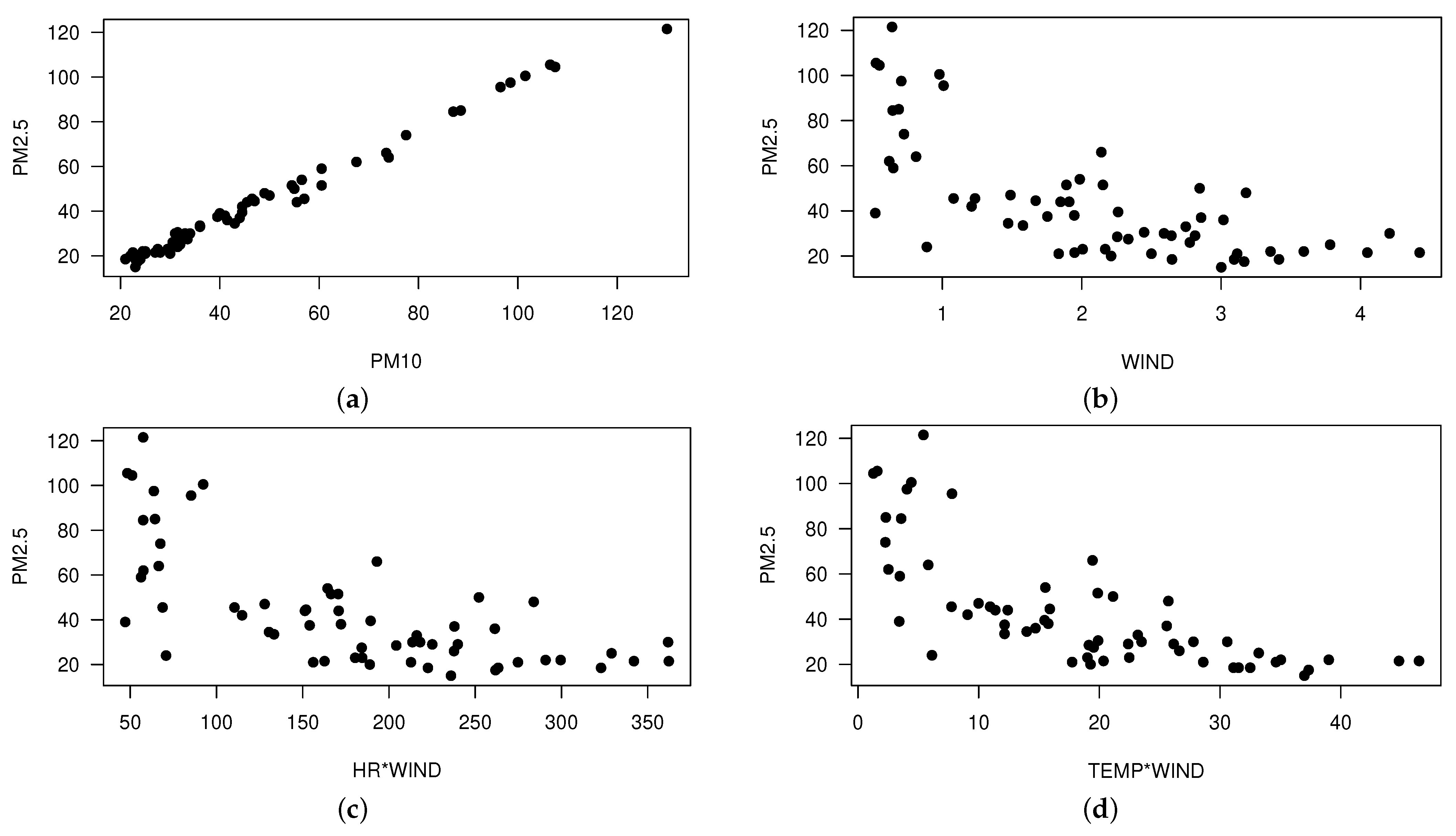
Figure 2 shows a correlation matrix for PM2.5, PM10, TEMP, WIND, and HR. From this figure, we detect: (i) a high positive association between PM2.5 and PM10 (Pearson coefficient of correlation equal to 0.99); (ii) medium negative association between PM2.5 and TEMP and WIND (Pearson coefficient of correlation equal to −0.70); (iii) low positive association between PM2.5 and HR (Pearson coefficient of correlation equal to 0.38). In Figure 3, scatter plots depicting the explanatory variables, response variable, and potential interactions among the explanatory variables are presented. In Figure 3a, note that the relationship between PM2.5 and PM10 is linear, while in Figure 3b, the relationship between PM2.5 and WIND is not linear. Furthermore, Figure 3c,d imply that the explanatory variables TEMP and HR may be engaging with the WIND variable in a nonlinear manner.

5.2. Parameter Estimation

Based on the EDA and the observed relationships between the median PM2.5 concentration and the variables as PM10, WIND, TEMP, and HR, we suggest the following varying-coefficients quantile regression models to capture the trends:

$${\sqrt{Q}}_i={\mathit{w}}_i^{\top }\mathit{\alpha }+x_{1i}{\beta }_1\left(t_i\right)+x_{2i}{\beta }_2\left(t_i\right),i\in \{1,2,\dots ,61\}$$

(10)

where $y_i\sim \mathrm{QLS}(Q_i,\varphi ,g)$ with Student-$t$ and normal PDF generator $g$, $\mathit{\beta }$ represents the vector of regression coefficients, while ${\mathit{w}}_i^{\top }={(1,w_{1i})}^{\top }$ with $w_{1i}$ denoting the values of the parametric covariate for the $i$th observation (PM10). The coefficients ${\beta }_k(\mathrm{for}k\in \{1,2\})$ correspond to unknown, smooth, and arbitrary functions of the explanatory variable $t_i$ (WIND), which are linked to the explanatory variables $x_{1i}$ (TEMP) and $x_{2i}$ (HR) from the $i$th case. These varying-coefficients quantile regression models allow for a more flexible and comprehensive characterization of the relationships between the median PM2.5 concentration and the other variables, considering potential variations across quantiles.

Table 2. MPL estimates, SEs, $p$-values, AIC and selected smoothing parameters and $\mathrm{df}(·)$ of the indicated model.

Model	Parameter	Estimate	SE	p-Value	AIC
Log-normal	${\alpha }_0$	3.072	2.2 × 10${}^{-5}$	<0.001	374.1
	${\alpha }_1$	0.068	1.1 × 10${}^{-3}$	<0.001
	$\varphi$	0.013	4.1 × 10${}^{-6}$
	${\lambda }_1$	4034.3
	${\lambda }_2$	2.2 × 10${}^5$
	df(${\lambda }_1$)	4.001
	df(${\lambda }_2$)	4.466
Log-$t$($\nu =4$)	${\alpha }_0$	3.052	1.7 × 10${}^{-5}$	<0.001	361.3
	${\alpha }_1$	0.070	8.3 × 10${}^{-4}$	<0.001
	$\varphi$	0.007	4.9 × 10${}^{-6}$
	${\lambda }_1$	4034.3
	${\lambda }_2$	5.9 × 10${}^5$
	df(${\lambda }_1)$	4.556
	df(${\lambda }_2$)	4.198

presents the MPL estimates for the model parameters, their approximate standard errors (SEs), $p$-values obtained from a $z$-test, the AIC, selected smoothing parameters, and the degrees of freedom $\mathrm{df}(·)$ for the models defined by Equation (10). The best values of ${\lambda }_1$ and ${\lambda }_2$ were selected by considering a grid of values and choosing those that yielded a range of $\mathrm{df}\left({\lambda }_1\right)$ and $\mathrm{df}\left({\lambda }_2\right)$ within the range of (4, 12), while minimizing the AIC value.

When comparing the results reported in Table 2, we observe that the estimates for ${\alpha }_0$ and ${\alpha }_1$ show similarity between both models, but the log-$t$ model has smaller estimated standard errors (SEs) for these parameters compared to the log-normal model. Additionally, the estimated value of $\varphi$ in the log-$t$ model is smaller than that in the log-normal model. It is worth noting that based on the (AIC), the log-$t$ model is preferred as it yields a lower AIC value.

To assess the distributional assumption made in the model, we examine the goodness-of-fit plots based on generalized Cox-Snell (GCS) residuals, as shown in Figure 4. Additionally, we provide the $p$-values associated with the Kolmogorov–Smirnov (KS) test, which are 0.73 for the log-normal model and 0.89 for the log-$t$($\nu =4$) model. Based on the goodness-of-fit plots, the KS test, and the AIC, we can conclude that the log-$t$($\nu =4$) model provides a better fit to the dataset. The log-$t$ model captures the underlying distribution of the data more accurately compared to the log-normal model, as indicated by the higher $p$-value and better fit observed in the goodness-of-fit plots.

Figure 5 displays the plots of the partial residuals relative to the WIND covariate, with the superimposed estimated smooth functions ${\beta }_1$ (on the left) and ${\beta }_2$ (on the right). The behavior of the partial residuals (dots) in these plots appears reasonable, indicating that the fit of the log-$t$($\nu =4$) varying-coefficients quantile regression model to the pollution dataset is adequate. The dots are closely aligned with the estimated curves, as expected, suggesting that the model captures the relationship between the WIND covariate and the partial residuals effectively. This agreement between the partial residuals and the estimated curves supports the appropriateness of the log-$t$($\nu =4$) varying-coefficients quantile regression model for analyzing the pollution data.

5.3. Diagnostic Analysis

In this section, we investigate the potential influence of individual observations using the local influence method for the selected varying-coefficients quantile regression model. We consider four perturbation schemes: case-weight perturbation, response variable perturbation, power parameter perturbation, and explanatory variable perturbation. Additionally, we examine the GL to assess the influence of each observed value on its own predicted value. These analyses allow us to identify potentially influential cases and understand their impact on the selected model. Details on the local influence method and the perturbation schemes can be found in Section 4.2.

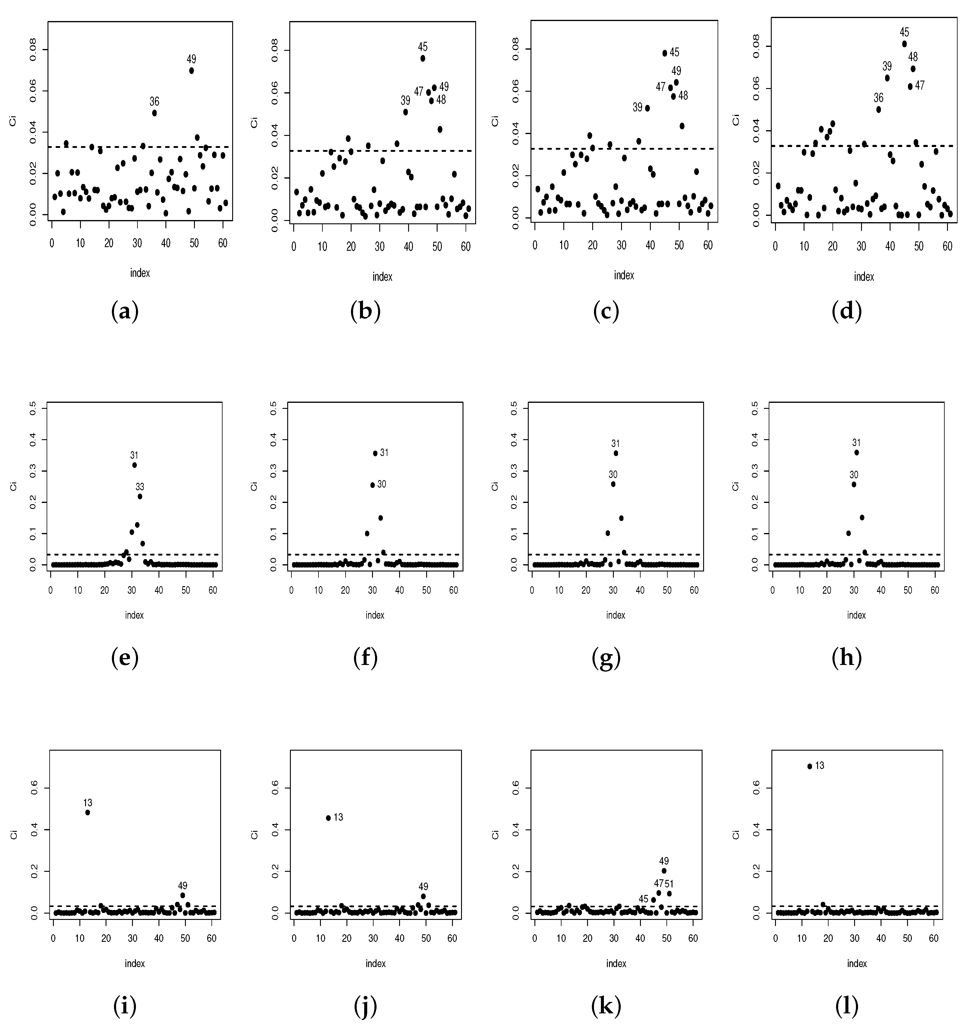
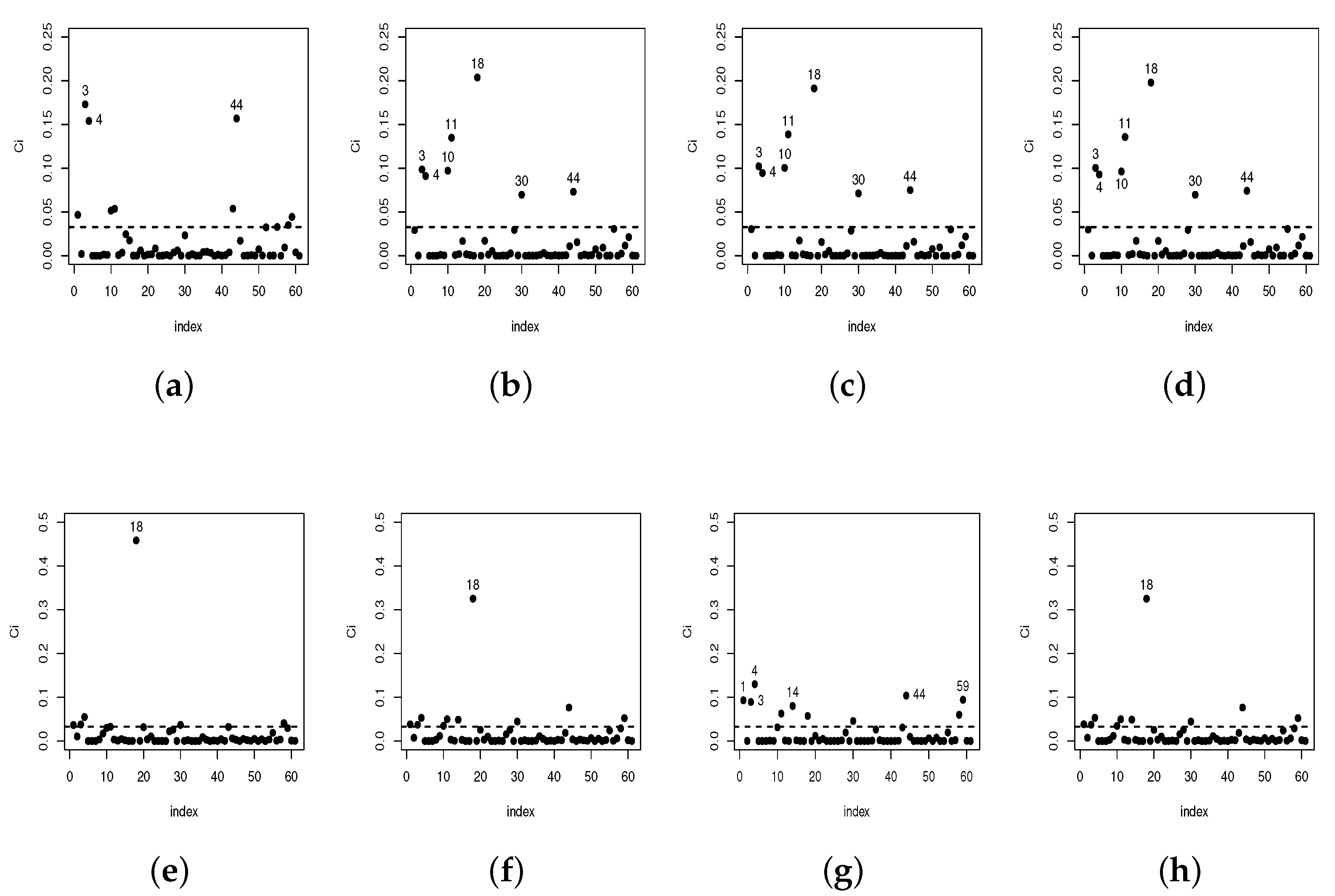
In Figure 6, we present index plots illustrating C${}_i$($\mathit{\theta }$) as defined in Section 4.2 for $\mathit{\alpha }$, ${\mathit{\beta }}_1$, ${\mathit{\beta }}_2$ and $\varphi$ under the case-weight perturbation (a,b,c,d), under response perturbation (e,f,g,h) and perturbation on the power parameter (i,j,k,l) schemes. Also, Figure 7 showcases the index plots of C${}_i$($\mathit{\theta }$) when introducing perturbations in covariates $X_1$ (a, b, c, d) and $X_2$ (e, f, g, h). Despite different observations being detected as potentially influential, it is worth noting that there are four cases (#13, #18, #31, and #45) that consistently appear as potentially influential across multiple perturbation schemes. These cases exhibit characteristics that make them stand out and have a notable impact on the model results.

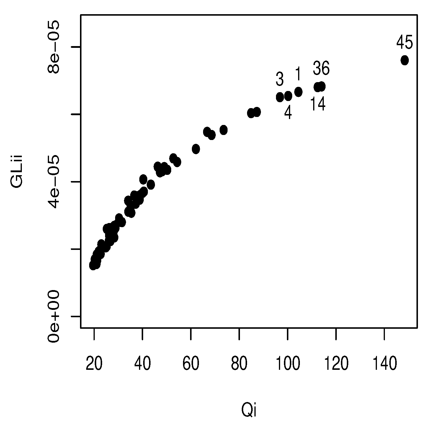
Figure 8 displays the GL plot, which assesses the influence of each observation on its own predicted value. From this plot, we observe that cases #45, #36, #14, #1, #3, #4 are potentially leverage points. These observations have response variable values that can exert a significant influence on their own predicted values. It is worth noting that these cases correspond to the outliers identified by the boxplot in Figure 1b. Their extreme values contribute to their influential nature within the model.

It is interesting to observe that the cases identified as potentially influential in the parametric component may not necessarily be detected in the nonparametric component, and vice versa. This indicates that different aspects of the data and model may be driving their influence in different ways. Additionally, the local influence analysis technique has successfully detected some atypical cases that were previously identified as outliers in Figure 1b. This reinforces the effectiveness of the local influence method in identifying observations that have a considerable impact on the model.

In the sense of evaluating the impact of these observations in the selected model, the subsets of cases {#13}, {#18}, {#31}, {#45}, {#13, #18}, {#13, #31}, {#13, #45}, {#18, #31}, {#18, #45}, {#31, #45}, and {#13, #18, #31}, {#13, #18, #45}, {#18, #31, #45} and {#13, #18, #31, #45} are removed and the model parameters are re-estimated. To determine the variation in the estimates of model parameters, we use the value of the relative changes (RCs) for each parameter. The RCs for each estimated parameter are calculated using the formula: ${\mathrm{RC}}_{\theta }=|\left({\widehat{\theta }}_j-{\widehat{\theta }}_{j\left(i\right)}\right)/{\widehat{\theta }}_j|\times 100\%,$ where ${\widehat{\theta }}_j$ represents the MPLE of ${\theta }_j$, and ${\widehat{\theta }}_{j\left(i\right)}$ represents the MPLE of ${\theta }_j$ after removing the subset $i$ of observations. Here, $j=1,2,3$ with ${\theta }_1={\alpha }_0$, ${\theta }_2={\alpha }_1$, and ${\theta }_3=\varphi$.

Table 3. RC (in %) on the MPL estimate of ${\alpha }_j$ and $\varphi$ and respective $p$-values (in parenthesis) for varying-coefficients quantile regression model after removing the indicated sets of cases.

	Parameters			Relative Changes
Removed Case	${\mathit{\alpha }}_{\mathbf{0}}$	${\mathit{\alpha }}_{\mathbf{1}}$	$\mathit{\varphi }$	RC${}_{{\mathit{\alpha }}_{\mathbf{0}}}$	RC${}_{{\mathit{\alpha }}_{\mathbf{1}}}$	RC${}_{\mathit{\varphi }}$
none	3.052	0.069	0.007
	(<0.001)	(<0.001)
{#13}	3.213	0.066	0.007	5.1%	4.7%	4.0%
	(<0.001)	(<0.001)
{#18}	2.961	0.072	0.006	3.0%	3.4%	5.5%
	(<0.001)	(<0.001)
{#31}	3.095	0.069	0.007	1.4%	1.1%	3.9%
	(<0.001)	(<0.001)
{#45}	2.891	0.073	0.006	5.3%	5.6%	4.0%
	(<0.001)	(<0.001)
{#13, #18}	3.415	0.065	0.006	11.9%	6.7%	18.0%
	(<0.001)	(<0.001)
{#13, #31}	3.223	0.066	0.006	5.6%	4.7%	9.4%
	(<0.001)	(<0.001)
{#13, #45}	3.093	0.069	0.006	1.4%	0.4%	13.0%
	(<0.001)	(<0.001)
{#18, #31}	3.011	0.071	0.006	1.3%	2.2%	9.5%
	(<0.001)	(<0.001)
{#18, #45}	2.901	0.073	0.006	4.9%	5.4%	10.9%
	(<0.001)	(<0.001)
{#13, #18, #31}	3.488	0.064	0.005	14.3%	7.8%	20.5%
	(<0.001)	(<0.001)
{#13, #18, #45}	3.005	0.071	0.006	1.5%	2.8%	17.4%
	(<0.001)	(<0.001)
{#18, #31, #45}	2.960	0.072	0.006	3.0%	4.0%	14.5%
	(<0.001)	(<0.001)
{#13, #18, #31, #45}	3.046	0.071	0.005	0.2%	1.9%	21.4%
	(<0.001)	(<0.001)

reports the values of RCs for the varying-coefficients quantile regression model after removing the indicated sets of cases. In this table, the individual elimination of cases #13 and #45 produces a RC in ${\alpha }_0$ and ${\alpha }_1$ of 5.1%, 4.7% and 5.3%, 5.6%, respectively, while the elimination of case #18 produces an RC in $\varphi$ of 5.5%. In addition, note that set of cases {#13, #18} and {#13, #18, #31} produces the largest RCs in ${\alpha }_0$, ${\alpha }_1$ and $\varphi$.

During the analyzed period, it was observed that observation #45 had particularly high concentrations of PM2.5 and PM10 compared to other observations. On the other hand, observation purple #31 had a very low wind speed, close to the minimum recorded during the entire period. These observations exhibit extreme values in their respective covariates. When the sets of potentially influential cases {#13, #18, #31, #45} are excluded from the analysis, it is observed that their removal results in notable alterations solely in the estimation of $\varphi$, displaying a percentage change of 21.4%. This suggests that these observations have a notable influence on the estimation of the dispersion parameter $\varphi$ in the model.

Finally, in Table 3, while certain RCs exhibit considerable values, there are no substantial alterations in inference, as evidenced by the diminutive $p$-values (less than 0.001) associated with the parameter estimates. It is important to note that when observations detected as influential in the diagnostic plots are eliminated, it can lead to significant changes in the parameter estimates. This indicates that the well-known robustness properties of maximum likelihood estimates from Student-t models may not necessarily apply to other perturbation schemes. Therefore, it is crucial to conduct diagnostic examinations specific to each case to properly assess the influence of observations and ensure the reliability of the model estimates.

6. Discussion, Conclusions and Future Research

In this work, we propose new varying-coefficients semiparametric quantile regression models based on the family of log-symmetric distributions, following the approach of [5,6,7]. By reparametrizing the family of log-symmetric distributions using a quantile, we introduce new quantile models that offer greater flexibility in modeling data compared to the model proposed by Saulo et al. [7], as a nonparametric component has been added (Section 2). We develop parameter estimation based on the penalized likelihood function and propose a back-fitting iterative algorithm implemented in the R language (Section 3). Additionally, we discuss diagnostic techniques for detecting potentially influential local observations and identifying leverage points (Section 4). Please note that the local influence analysis reinforces the need for diagnostic evaluation. It has been observed that parameter estimators in this class of models tend to be sensitive to the presence of atypical or influential data points. To the best of our knowledge, techniques for detecting leverage points have not been developed for semiparametric quantile regression models.

We illustrate the methodology developed in this work using data associated with PM2.5 pollution in Padre Las Casas city for predicting the daily median of 1-h average values. We propose and fit two models (log-normal and log-$t(\nu =4)$) and evaluate them using CGS residuals and their AIC values. The plots of CGS residuals and partial residuals show a good fit of the selected model (log-$t(\nu =4)$) to the data. We also apply our diagnostic techniques to detect potentially influential cases and leverage points (Section 4.2); however, no inferential changes are observed in the parameter estimates.

Thus, among the accomplishments of this work, we can highlight: (i) The development of novel quantile regression models suitable for modeling data following asymmetric distributions, which can be added into the existing toolkit for quantile modeling; (ii) The expansion of our model beyond the one presented in [7], incorporating nonlinear structures arising from interaction effects. (iii) The derivation of analytical tools for identifying potentially influential observations and leverage points.

One limitation of our study is that the proposed models may not be suitable for describing other types of data, such as temporally or spatially correlated data, as well as censored data. In such cases, the utilization of multivariate distributions for the response variable, reparametrized by quantiles of marginal distributions, may be necessary. Another area for future investigation is conducting a simulation study to evaluate the distributional behavior of the residuals used in this study and exploring alternative types of residuals appropriate for this type of regression. This aspect has received limited attention in the existing literature. Furthermore, we aim to establish inferences about the model parameters through asymptotic analysis of specific estimators. Lastly, we intend to compare our model with others, including models proposed by [7,12]. These are additional areas that remain unexplored, and we plan to address these open questions in our future research.

References

1. Vanegas, L.; Paula, G. A semiparametric approach for joint modeling of median and skewness. Test 2015, 24, 110–135. [Google Scholar] [CrossRef]
2. Arellano-Valle, R.B.; Gómez, H.W.; Quintana, F.A. A New Class of Skew-Normal Distributions. Commun. Stat. Theory Methods 2004, 33, 1465–1480. [Google Scholar] [CrossRef]
3. Paula, G.A.; Leiva, V.; Barros, M.; Liu, S. Robust statistical modeling using the Birnbaum-Saunders-t distribution applied to insurance. Appl. Stoch. Model. Bus. Ind. 2012, 28, 16–34. [Google Scholar] [CrossRef]
4. Leiva, V.; Santos-Neto, M.; Cysneiros, F.J.A.; Barros, M. Birnbaum–Saunders statistical modelling: A new approach. Stat. Model. 2014, 14, 21–48. [Google Scholar] [CrossRef]
5. Sánchez, L.; Leiva, V.; Galea, M.; Saulo, H. Birnbaum-Saunders quantile regression and its diagnostics with application to economic data. Appl. Stoch. Model. Bus. Ind. 2021, 37, 53–73. [Google Scholar] [CrossRef]
6. Sánchez, L.; Leiva, V.; Marchant, C.; Saulo, H.; Sarabia, J.M. A new quantile regression model and its diagnostic analytics for a Weibull distributed response with applications. Mathematics 2021, 9, 2768. [Google Scholar] [CrossRef]
7. Saulo, H.; Dasilva, A.; Leiva, V.; Sanchez, L.; de la Fuente-Mella, H. Log-symmetric quantile regression models. Stat. Neerl. 2022, 76, 124–163. [Google Scholar] [CrossRef]
8. Vanegas, L.; Paula, G. Log-symmetric distributions: Statistical properties and parameter estimation. Braz. J. Probab. Stat. 2016, 30, 196–220. [Google Scholar] [CrossRef]
9. Vanegas, L.; Paula, G. An extension of log-symmetric regression models: R codes and applications. J. Stat. Simul. Comput. 2016, 86, 1709–1735. [Google Scholar] [CrossRef]
10. Ventura, M.; Saulo, H.; Leiva, V.; Monsueto, S.E. Log-symmetric regression models: Information criteria and application to movie business and industry data. Appl. Stoch. Model. Bus. Ind. 2019, 35, 963–977. [Google Scholar] [CrossRef]
11. Hao, L.; Naiman, D.Q. Quantile Regression; Sage Publications: London, UK, 2007. [Google Scholar]
12. Koenker, R.; Chernozhukov, V.; He, X.; Peng, L. Handbook of Quantile Regression; CRC Press: Boca Raton, FL, USA, 2018. [Google Scholar]
13. Noufaily, A.; Jones, M.C. Parametric quantile regression based on the generalized gamma distribution. J. R. Stat. Soc. Ser. 2013, 62, 723–740. [Google Scholar] [CrossRef]
14. Hastie, T.; Tibshirani, R. Generalized Additive Models; Chapman and Hall: New York, NY, USA, 1990. [Google Scholar]
15. Green, P.J.; Silverman, B.W. Nonparametric Regression and Generalized Linear Models; Chapman and Hall: Boca Raton, FL, USA, 1994. [Google Scholar]
16. Ibacache-Pulgar, G.; Paula, G.A.; Cysneiros, F.J.A. Semiparametric additive models under symmetric distributions. Test 2013, 22, 103–121. [Google Scholar] [CrossRef]
17. Ramires, T.; Ortega, E.; Hens, N.; Cordeiro, G.; Paula, G. A flexible semiparametric regression model for bimodal, asymmetric and censored data. J. Appl. Stat. 2018, 45, 1303–1324. [Google Scholar] [CrossRef]
18. Manghi, R.; Cysneiros, F.J.A.; Paula, G. Generalized additive partial linear models for analyzing correlated data. Comput. Stat. Data Anal. 2019, 129, 47–60. [Google Scholar] [CrossRef]
19. Oliveira, R.A.; Paula, G.A. Additive models with autoregressive symmetric errors based on penalized regression splines. Comput. Stat. 2021, 36, 2435–2466. [Google Scholar] [CrossRef]
20. Ferreira, C.; Montoril, M.; Paula, G. Partially linear models with p-order autoregressive skew-normal errors. Braz. J. Probab. Stat. 2022, 36, 792–806. [Google Scholar]
21. Cardozo, C.A.; Paula, G.A.; Vanegas, L.H. Generalized log-gamma additive partial linear models with P-spline smoothing. Stat. Pap. 2022, 63, 1953–1978. [Google Scholar] [CrossRef]
22. Cavieres, M.F.; Leiva, V.; Marchant, C.; Rojas, F. A methodology for data-driven decision making in the monitoring of particulate matter environmental contamination in Santiago of Chile. Rev. Environ. Contam. Toxicol. 2020, 250, 5–67. [Google Scholar]
23. Ibacache-Pulgar, G.; Reyes, S. Local influence for elliptical partially varying coefficient model. Stat. Model. 2018, 18, 149–174. [Google Scholar] [CrossRef]
24. Good, I.J.; Gaskins, R.A. Nonparametric roughness penalties for probability densities. Biometrika 1971, 58, 255–277. [Google Scholar] [CrossRef]
25. Silverman, B.W. Some aspects of the spline smoothing approach to non-parametric regression curve fitting. J. R. Stat. 1985, 47, 1–52. [Google Scholar] [CrossRef]
26. Green, P.J. Penalized likelihood for general semi-parametric regression models. Int. Stat. Rev. 1987, 55, 245–259. [Google Scholar] [CrossRef]
27. Adams, R.A.; Fournier, J. Sobolev Spaces. In Pure and Applied Mathematics; Academic Press: Boston, MA, USA, 2003. [Google Scholar]
28. Rigby, R.A.; Stasinopoulos, D.M. Generalized additive models for location, scale and shape. J. R. Stat. Soc. Ser. (Appl. Stat.) 2005, 54, 507–554. [Google Scholar] [CrossRef]
29. Berhane, K.; Tibshirani, J. Generalized additive models for longitudinal data. Can. J. Stat. 1998, 26, 517–535. [Google Scholar] [CrossRef]
30. Cook, R.D. Assessment of local influence (with discussion). J. R. Stat. Soc. 1986, 48, 133–169. [Google Scholar]
31. Escobar, L.; Meeker, W. Assessing influence in regression analysis with censored data. Biometrics 1992, 48, 507–528. [Google Scholar] [CrossRef]
32. Wei, B.C.; Hu, Y.Q.; Fung, W.K. Generalized leverage and its applications. Scand. J. Stat. 1998, 25, 25–37. [Google Scholar] [CrossRef]
Figure 1. Histogram with density kernel estimation (solid black line) (a) and boxplot (b) for median PM2.5 concentrations recorded by Padre Las Casas AQMS during June–July 2020.
Axioms 12 00976 g001
Figure 2. Correlation matrix displaying the respective Pearson correlation coefficient for the specified explanatory and response variables.
Axioms 12 00976 g002
Figure 3. Scatter plots for median PM2.5 vs. PM10 concentrations (a); median PM2.5 vs. WIND (b); median PM2.5 vs. HR*WIND (c); and, median PM2.5 vs. TEMP*WIND (d) recorded by Padre Las Casas AQMS during June–July 2020.
Axioms 12 00976 g003
Figure 4. Goodness-of-fit plots with simulated envelope for GCS residual under the indicated model with the analyzed data set.
Axioms 12 00976 g004
Figure 5. Plots of partial residuals in relation to the WIND covariate, with the estimated smooth functions β 1 (on the left) and β 2 (on the right) superimposed.
Axioms 12 00976 g005
Figure 6. Case weight (ad), response (eh) and on the power parameter (il) perturbation for α , β 1 , β 2 and ϕ .
Axioms 12 00976 g006
Figure 7. Perturbationin the covariate X 1 (ad) and X 2 (eh) scheme for α , β 1 , β 2 and ϕ .
Axioms 12 00976 g007
Figure 8. Generalized leverage.
Axioms 12 00976 g008