Abstract
This paper deals with the mathematical modelling of the red palm weevil (RPW), Rhynchophorus ferrugineus (Olivier) (Coleoptera: Curculionidae), in date palms using chemical control by utilizing injection and sex pheromone traps. A deterministic and stochastic model for RPW is proposed and analyzed. The existence of a positive global solution for the stochastic RPW model is investigated, and the conditions for the extinction of RPWs from the stochastic system are obtained. The adequate criteria for the presence of a unique ergodic stationary distribution for the RPW system are established by creating suitable Lyapunov functions. The impact of chemical injection and pheromone traps on RPW is demonstrated. The importance of environmental noise on RPW is highlighted and simulated using the Milstein method.
Keywords:
stochastic models; stability; sex pheromone trap; Rhynchophorus ferrugineus; chemical injection MSC:
37N25; 92D30; 93E03
1. Introduction
The red palm weevil (RPW) is considered one of the most dangerous insects to date palms. Recently, RPW expanded its distribution within palm varieties and outbreaks to be a major invasive agricultural pest in date palm cultivars, which helped in becoming a key date-palm pest within a short time [1]. RPW as an invasive species is defined by its ability to invade, colonize and adapt to new agricultural areas worldwide [2]. The global movement of commercial goods helped spread the species of RPW, which was previously confined to areas of its initial discovery in India [3,4]. The insect is voracious in feeding, especially in the larval stage, which requires at least 60–90 days to complete its development and transfer to a pupal stage. RPW is a soft tissue insect that feeds on the inner tissue of palm trunk [5,6,7,8]. Consequently, larvae feeding leads to severe damage, resulting in destroying the inner palm trunk and finally complete palm death. Reducing RPW feeding, damage and distribution is not possible to by following one control method, but an integrated control program must be developed to reduce RPW activity and limit its damage. The integrated management program for RPW should include different control techniques such as mechanical, chemical, biological control and other possible methods that can be relied upon to control the numbers of the RPW in the affected areas. When RPW damage is detected on the trunk at one or more points, the chemical injection method can be followed, and it is considered one of the most successful methods of treatment and is a more effective method than spraying pesticides [9,10,11]. According to [12], early and intermediate infestation can be treated by injecting insecticides into the trunk. When the trunk is locally injected, the chemical pesticide spreads within the stem under the influence of diffusion and gravity, which leads to the killing of both the larval and pupal stages. Sex aggregated pheromone traps are used to control the level of RPW in farms by attracting both males and females, which affects the pest populations and kills them because the traps contain insecticides that kill what is being caught, thus reducing the number of RPW [3,13]. The researchers showed that using pheromone traps for the RPW are one of the most effective ways to monitor and reduce the numbers of this harmful insect in the Arab Gulf countries [14]. Mathematical models can help understand and explain the spread of this pest and the methods and factors that control it. This paper aims to develop and analyze a mathematical model of RPW with sex pheromone traps and chemical injection. The paper is organized as follows: The RPW mathematical model is described in Section 2, and the conditions for stability of the RPW model are obtained. In Section 3, the stochastic RPW model is performed, and the existence of a positive global solution for the stochastic RPW model is investigated, as well as the sufficient conditions for population extinction from the stochastic system. Sufficient criteria for the existence of a unique ergodic stationary distribution for the RPW system are established. The numerical simulations described in Section 4 are used to verify the theoretical results. The discussion and conclusion are found in Section 5.
2. Mathematical Model
- In this model, the total date palm tree population is divided into two classes: susceptible date palm tree denoted by and infected date palm denoted by . In the absence of RPW, the date palm tree grows logistically with an intrinsic growth rate r and carrying capacity k. The natural death rate of the susceptible and infected date palm tree is .
- Assume that the date palm tree is susceptible to infection according to simple mass kinematics with as the RPW transmission coefficient. Experimental studies on palm pests indicated that the functional response pattern of the predator is consistent with the Holling II functional response [15,16]. As a result, we assume that RPW larvae harvest palm trees with Holing type-II functional response. The predation rate of RPW larvae on a date palm tree is c, and constant a is the half-saturation constant. The larvae population decreases by rate due to the transformation from the larva stage to the adult stage. The transition rate of RPW larvae to adults females is given by , whereas a complementing fraction will emerge as males . We assume that larvae decreases at the rate due to the injection of chemical compounds. The natural death of larvae is assumed to be , while the natural death for adult RPW is .
- To indicate the trap’s effect, one can consider the approach proposed by Barclay [17]. We assume the pheromone trap attracted additional females. As a result, the RPW males attracted to pheromone traps according to , where represents the effective rate of pheromone traps on mortality of RPW males. Recently, this approach was used by [18,19,20,21] to investigate the dynamics of the mirid population under mating disruption and trapping.
The following system describes the model of RPW with sex pheromone traps and chemical injection.
The RPW model (1) has four equilibrium points. The trivial equilibrium point is stable if . The free RPW equilibrium point exists if and stable if , where . The equilibrium point , where and . exists if . The first three eigenvalues of are , and , where . The other two eigenvalues are given by and the roots have negative real parts. As a result, is stable if The coexistence equilibrium point , where
exists if and , where . The stability of the RPW system around is now investigated. The Jacobian matrix of the RPW model (1) around is given as follows.
The first two eigenvalues of are , and . The other three eigenvalues are determined by where , and . The coexistence equilibrium point is stable if and .
3. Dynamics of the Stochastic Model
Stochastic effects can be significant in the case of RPW because the environmental conditions of its transmission are subject to randomness. The deterministic RPW (1) ignores the possible importance of a stochastic environment. In [22], a deterministic and stochastic prey–predator model for three predators and a single prey was proposed and analyzed. In this paper, we study a stochastic eco-epidemiological model for one of the agricultural pests. The RPW model (1) will be extended to include the stochastic effects as follows:
where represents the five-dimensional standard Brownian motions with , and is the intensities of the white noise defined in a complete probability space with a filtration satisfying the usual conditions. In the next theorem, we will prove the existence and uniqueness of a global positive solution of the system (2). This approach has recently been used in many papers for the analysis of stochastic predator–prey systems [23,24,25,26,27], stochastic epidemic models [28,29,30,31,32,33,34] and stochastic eco-epidemiological models [35].
Theorem 1.
For any given initial value , there exists a unique solution of system (2) for and the global positive solution remains in with probability one.
Proof.
Firstly, one can consider the local solution of system (2) for , where is the explosion time [36], by conducting the transformation of variables.
Using the Itô formula, one can change system (2) as follows.
The coefficients of system (3) satisfy the local Lipschitz conditions; consequently, there exists a unique local solution
on . To ensure that this solution is global, one needs to prove that a.s. Let be sufficiently large for every coordinate in the interval . For each integer , we define the stopping time.
One can note that is increasing as . Assume , then . In the next step, one needs to verify that . If this is not true, then there exists a constant and such that . As a result, there exists an integer such that . Define the following positive definite function as
Using Itô’s formula, one obtains
Using inequality , for any , one obtains
which means that
where , and .
Taking the expectation of the above inequality, one obtain the following.
Following [35,37], applying Grownwall’s inequality, one obtains
The remainder of the proof is similar to [37,38] and is therefore omitted. The proof is now complete. □
The above theorem shows that the stochastic RPW system (2) has a positive global solution remaining in with a probability of one. In the following, we will establish the boundedness property of the RPW model (2).
Lemma 1.
Let then for any positive initial value, the following inequality holds:
where.
Proof.
According to the stochastic RPW system (2), we have the following.
Integrating from 0 to t yields
According to strong law of large numbers, one obtains
Consequently,
Thus, one obtains
□
The above theorem tells us the solution of RPW system (2) is uniformly bounded in mean, and as a result, the deterministic RPW system (1) is uniformly bounded. The conditions for RPW extinction will be established using the following theorem.
Theorem 2.
If , then the populations will be extinct with a probability of one for any positive initial conditions.
Proof.
Applying Itô’s formula to the first equation of stochastic RPW system (2), one obtains
and integrating both sides of the above equation from 0 to t leads to
It follows that
which implies that
Applying Itô’s formula to the second equation of stochastic RPW system (2), one obtains
Consequently,
Taking the superior limit, one obtains
Thus, The other classes of the RPW system (2) also proceed to extinction a.s. Thus,
□
In the following theorem, we will establish the asymptotic stability of the RPW system (2).
Theorem 3.
If , , , , and , then the trivial solution of the RPW system (2) is stochastically asymptotically stable in probability for any positive initial conditions.
Proof.
Firstly, one can consider the following linearized RPW system.
Consider the following Lyapunov function.
Applying Itô’s formula to the linearized stochastic RPW system (4), one computes
can be written in the form , where and
Matrix Q will be negatively definite if , , , , and According to Theorem 2.4 [36], if there exists a positive-definite decreasing unbounded function such that is negative-definite, then the trivial solution of the linearized stochastic RPW system (4) is stochastically stable in the large. As indicated by Arnold [39] (Theorem 11.6.1), if the trivial solution of the linear stochastic RPW system (4) is stochastically asymptotically stable, then the trivial solution of the non-linear stochastic RPW system (2) is stochastically asymptotically stable. □
In the following, based on the method of Khasminskii [40], we establish the conditions for the existence of an ergodic stationary distribution of the positive solutions to the RPW model (2). The positive equilibrium for system (1) is locally asymptotically stable, but there is non positive equilibrium point for RPW system (2). According to [41,42], one can investigate the stationary distribution for the RPW system (2) instead of asymptotically stable equilibria. Before providing the main theorem, we first state the following Lemma
Lemma 2
([40]). The Markov process has a unique ergodic stationary distribution if there exists a bounded closed domain with regular boundary possessing the following properties:
- There is a positive number M such that
- There exists a non-negative function V such that is negative on
Theorem 4.
Assume , then for any positive initial value, system (2) has a unique ergodic stationary distribution
Proof.
In order to prove Theorem 4, one needs only to validate conditions and of Lemma 2. The first step is to validate conditions of Lemma 2. The diffusion matrix of the system (2) is given by
Following [37,43,44], choose ; then, there is a positive number such that
for all , This implies condition that in Lemma 2 is satisfied. The second step is to prove that there exists a non-negative function such that as follows. Define the following function.
Applying Itô formula leads to the following:
where
Define ; then, is negative on which implies that condition in Lemma 2 is satisfied. As a result, the RPW system (2) is ergodic and has a stationary distribution. This completes the proof. □
4. Numerical Simulations
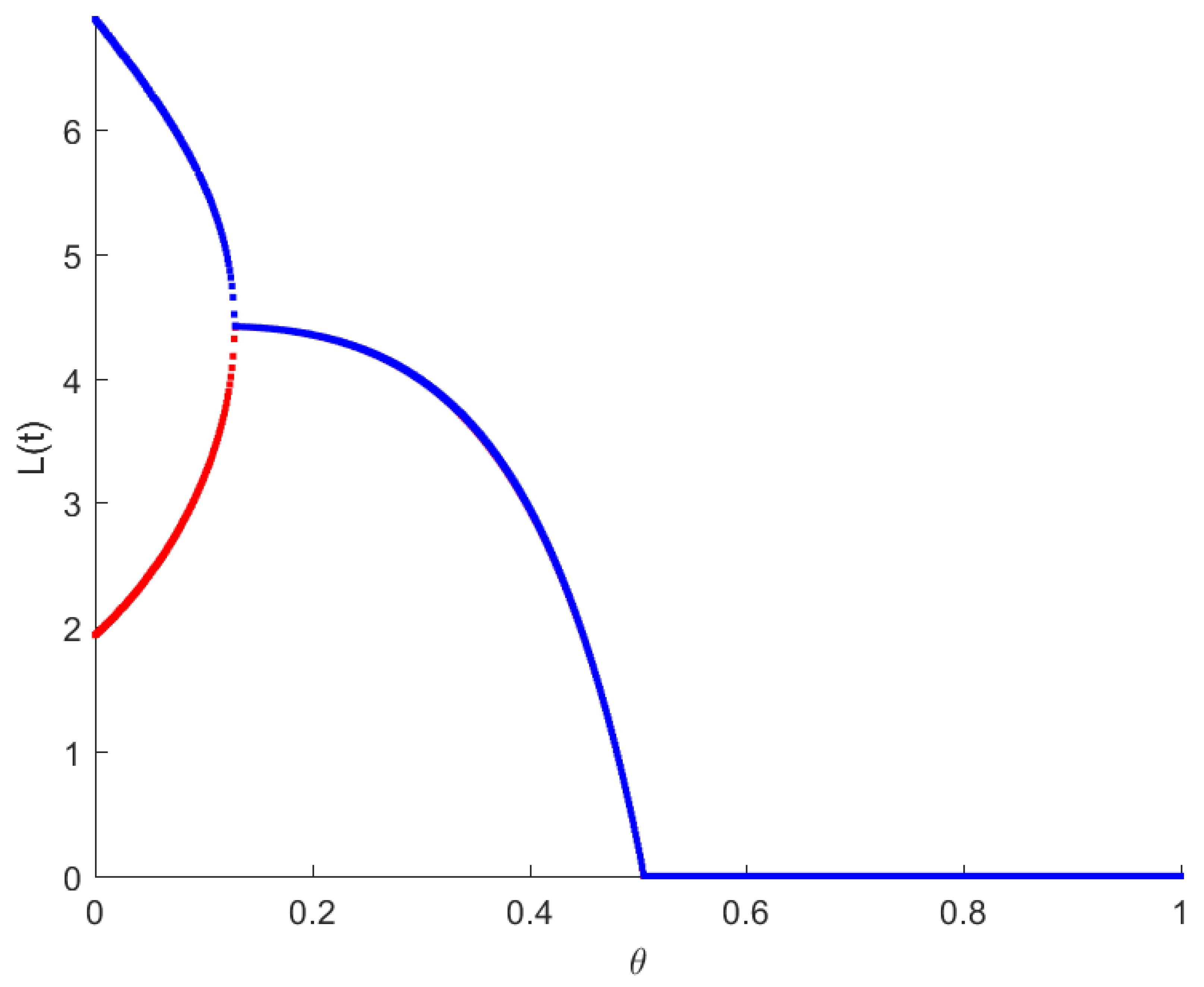
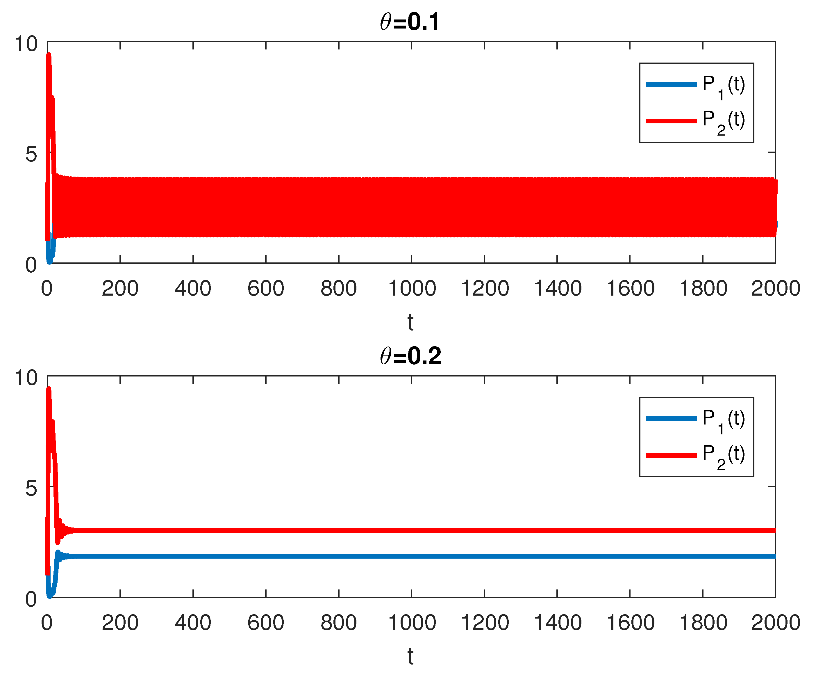
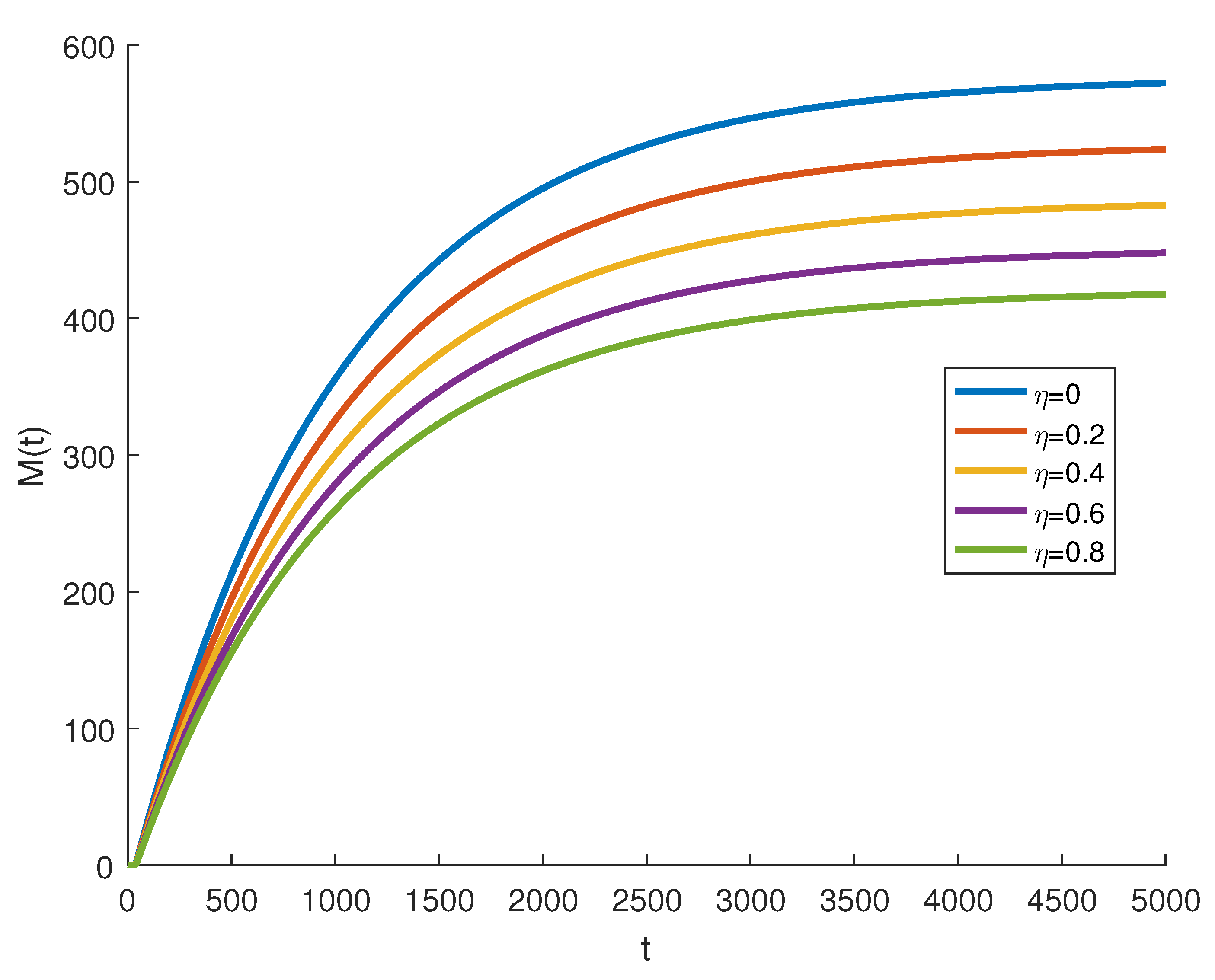
The RPW model is simulated in this section to demonstrate some of the previously obtained analytical results. The following parameters will be used to simulate the interactions between palm trees and different stages of the RPW To understand the effect of the chemical injection coefficient on the dynamic behavior of the RPW (1), one can increase the value and keep the rest of the parameters as above. Figure 1 indicates the occurrence of transcritical bifurcation at and supercritical Hoph bifurcation at , as shown in Figure 2. When , the density of larvae will become extinct; consequently, the other classes of RPW will be extinct. Figure 3 indicates that the population density of RPW males decreases with an increase in sex pheromone trap parameter . One can conclude that pheromone trap parameters can limit the spread of RPWs. The effect of intrinsic date palm growth rate r can be shown by drawing the bifurcation diagram regarding r as a bifurcation parameter. From Figure 4 and Figure 5, it can be seen that two transcritical bifurcation values localized at and . When , the trivial equilibrium point is locally asymptotically stable. For , the equilibrium point is locally stable. It can be seen that supercritical Hopf bifurcation value localized at as shown in Figure 5. When , the RPW model (2) proceeds through limit cycle oscillation and for , is locally stable as indicated in Figure 4 and coincides with Figure 5.
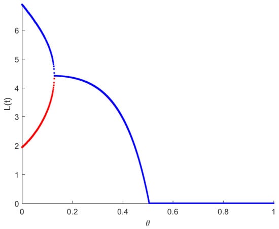
Figure 1.
Bifurcation diagram of RPW system (1) with respect to .
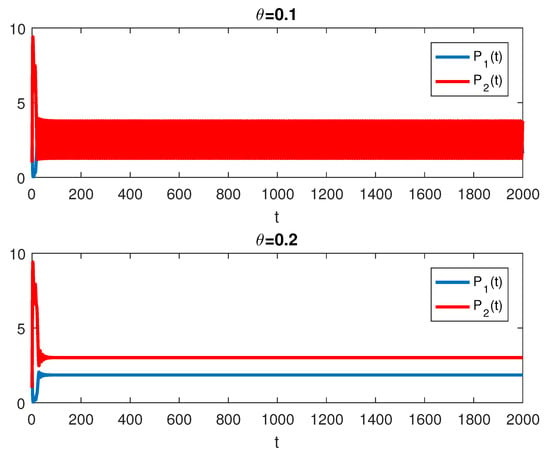
Figure 2.
The RPW system (1) with and .
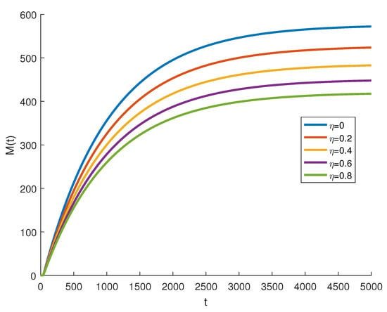
Figure 3.
The RPW system (1) with different values of .
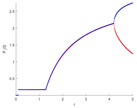
Figure 4.
Bifurcation diagram of RPW system (1) with respect to r.
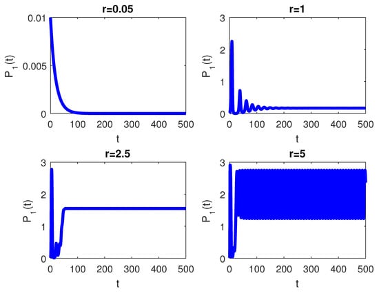
Figure 5.
The RPW system (1) with .
To provide some numerical findings to the stochastic RPW system (2), we use the Milstein method mentioned in [45]. The stochastic RPW system (2) reduces to the following discrete system:
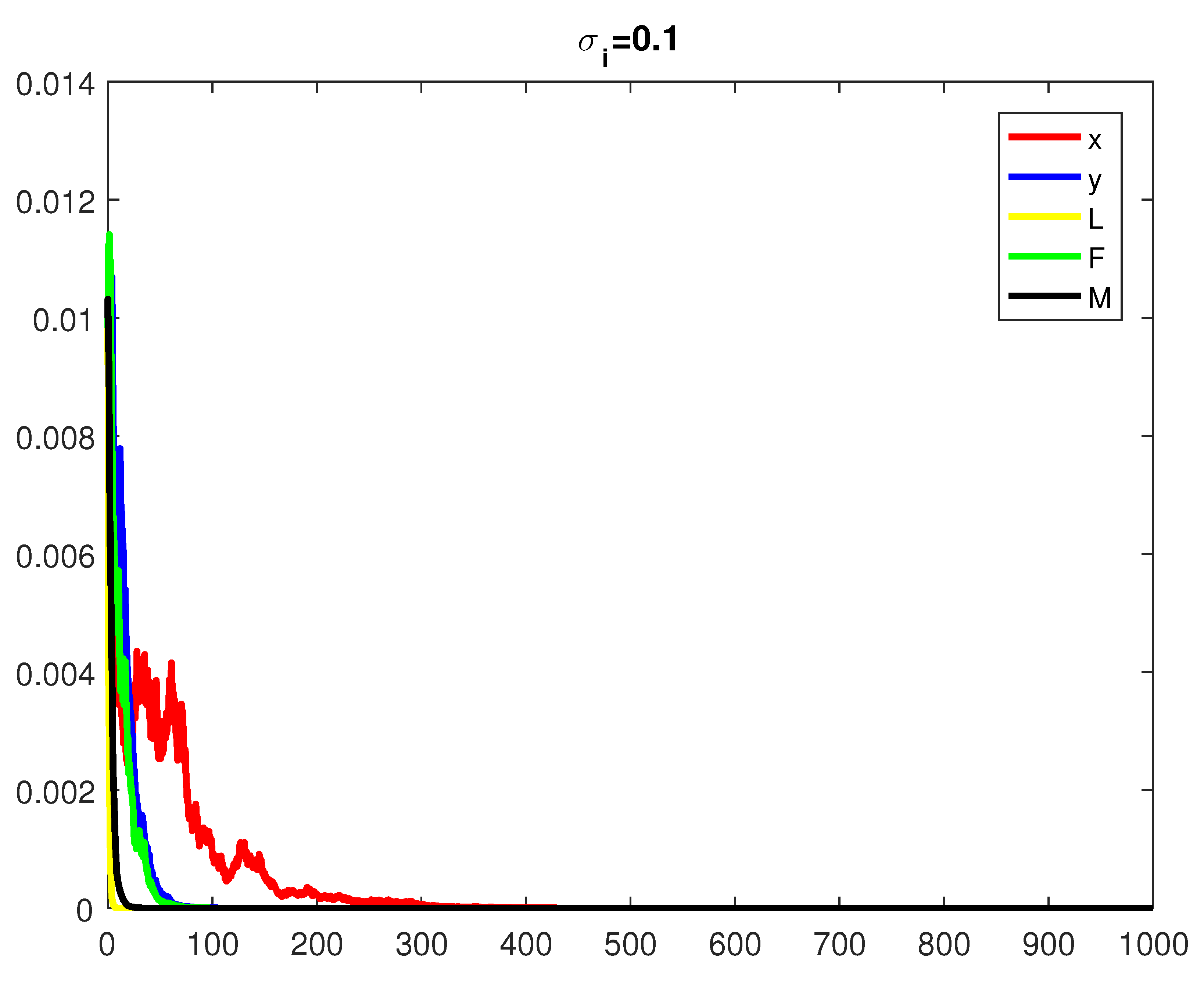
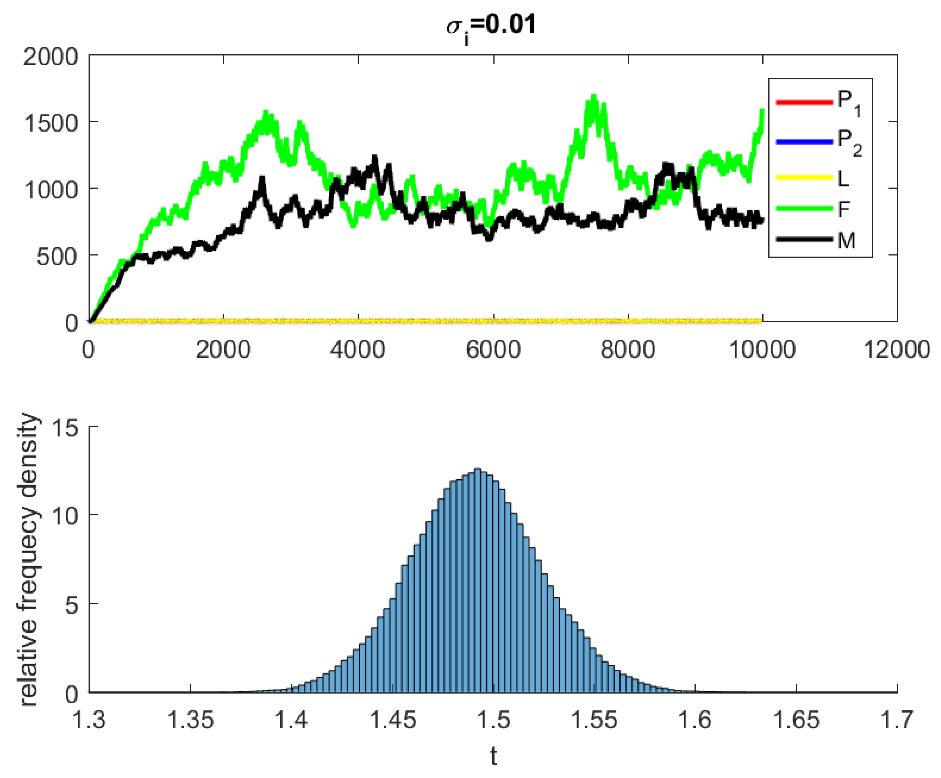
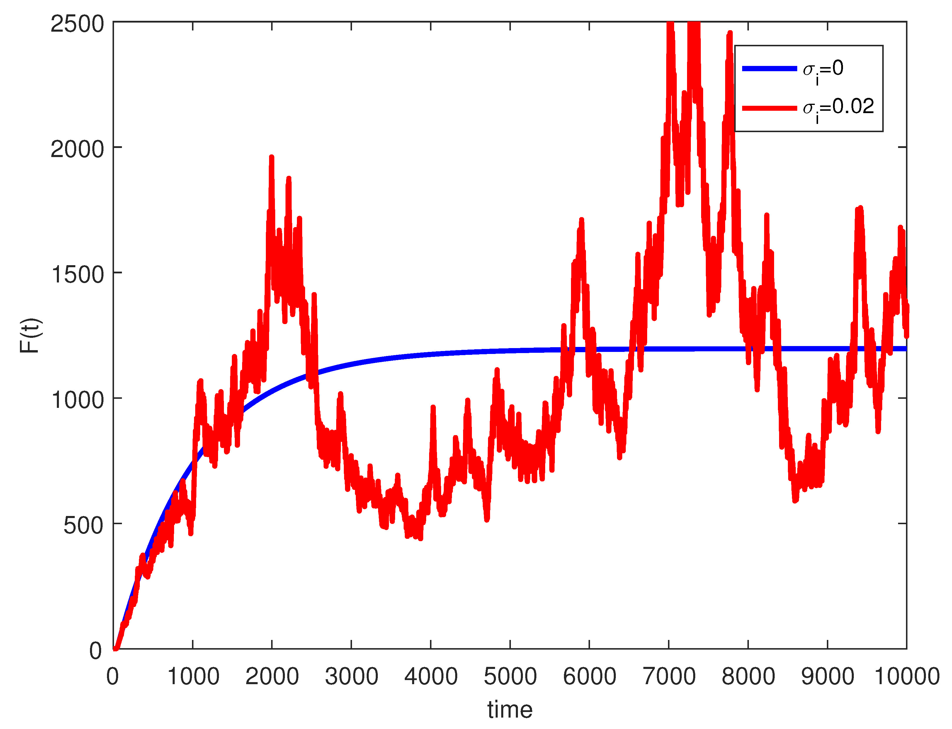
where are independent random Gaussian variables , and h is a positive time increment. For the given parameters, one can note that the conditions of Theorems 2 and 3 are verified and the populations will be extinct with probability one if as indicated in Figure 6, when . The time series for the stochastic system (2) and its histograms of probability density function are shown in Figure 7. The conditions of Theorem 3 hold and system (2) has a unique stationary distribution and it has ergodic properties. If one gradually increases the intensities of fluctuation and keeps the remaining parameters unchanged, the RPW female oscillates around coexistence point , as shown in Figure 8.
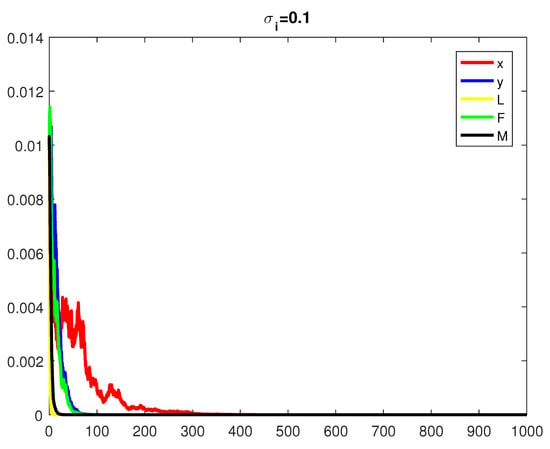
Figure 6.
The stochastic RPW system (2) with .
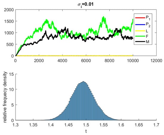
Figure 7.
The stochastic system (2) and its histograms of probability density function.
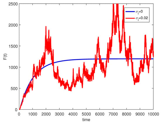
Figure 8.
The stochastic RPW system (2) with and .
5. Discussion and Conclusions
In this paper, a deterministic and stochastic model for RPW has been proposed and analyzed. For the deterministic model, the stability of the solution has been studied. The chemical injection parameter plays an essential role in controlling the RPW insect, because by increasing the rate of injection, the insect is killed in the larval stage, and as a result, the adult stages of the insect do not appear. The parameter is biologically important, as by knowing the parameters of the insect infestation of palm farms, it is possible to determine the critical injection rate that leads to the disappearance of the palm weevil from the farms. Moreover, from the numerical results, one can find that the population density of RPW males decreases with increasing sex pheromone trap parameters . The numerical simulation for RPW indicates that white noise has a significant impact on the dynamical behavior of the RPW system. The conditions for the extinction of RPW insects from the stochastic model have been obtained. The adequate criteria for the presence of a unique ergodic stationary distribution for the RPW system have been established by creating suitable Lyapunov functions. The importance of environmental noise in RPW has been simulated using the Milstein method. If one inserts the intensities of fluctuation and the chemical injection parameter , the results of the stochastic model in this paper coincide with the results of the deterministic model considered by [18]. Moreover, it is interesting to study controlling RPW in date palms using sterile insect technique and the effects of other factors, such as time delays and impulsive perturbations. We leave these cases for future work.
Author Contributions
Formal analysis, M.E.-S.; Funding acquisition, A.A.-N.; Methodology, M.E.-S.; Project administration, A.A.-N.; Supervision, N.F.A.-B.; Validation, M.E.-S., A.A.-N. and N.F.A.-B.; Writing—original draft, M.E.-S. All authors have read and agreed to the published version of the manuscript.
Funding
The authors gratefully acknowledge Qassim University, represented by the Deanship of Scientific Research, on the financial support under the number (cosao-bs-2019-2-2-I-5469) during the academic year 1440 AH/2019 AD.
Institutional Review Board Statement
Not applicable.
Informed Consent Statement
Not applicable.
Data Availability Statement
Data sharing is not applicable to this article as no datasets were generated or analyzed during the current study.
Conflicts of Interest
The authors declare that there is no conflict of interest.
References
- Abdel-Baky, N.F.; Hamed, K.E.; Al-Otaibi, N.D.; Aldeghairi, M.A. Bioassay of Some Indigenous Entomopathogens for Controlling Rhynchophorus ferrugineus, Olivier in Saudi Arabia. Pak. J. Biol. Sci. 2021, 24, 944–952. [Google Scholar] [CrossRef]
- Wang, G.; Hou, Y.; Zhang, X.; Zhang, J.; Li, J.; Chen, Z. Strong population genetic structure of an invasive species, Rhynchophorus ferrugineus (Olivier), in southern China. Ecol. Evol. 2017, 7, 10770–10781. [Google Scholar] [CrossRef] [PubMed]
- Abd El-Wahab, A.; Abd El-Fattah, A.; El-Shafei, W.; El Helaly, A. Efficacy of aggregation nano gel pheromone traps on the catchability of Rhynchophorus ferrugineus (Olivier) in Egypt. Braz. J. Biol. 2020, 81, 452–460. [Google Scholar] [CrossRef] [PubMed]
- Faleiro, J.; Abdallah, A.B.; El-Bellaj, M.; Al-Ajlan, A.; Oihabi, A. Threat of the red palm weevil, Rhynchophorus ferrugineus (Olivier) to date palm plantations in North Africa. Arab. J. Plant Prot. 2012, 30, 274–280. [Google Scholar]
- Nangai, V.L.; Martin, B. Interpreting the acoustic characteristics of RPW towards its detection-A review. In Proceedings of the IOP Conference Series: Materials Science and Engineering, Narsimha Reddy Engineering College, Hyderabad, India, 3–4 July 2017; Volume 225, p. 012178. [Google Scholar]
- Al-Dosary, N.M.; Al-Dobai, S.; Faleiro, J.R. Review on the management of red palm weevil Rhynchophorus ferrugineus Olivier in date palm Phoenix dactylifera L. Emir. J. Food Agric. 2016, 28, 34–44. [Google Scholar] [CrossRef]
- Archer, L.; Crane, J.H.; Albrecht, U. Trunk Injection as a Tool to Deliver Plant Protection Materials—An Overview of Basic Principles and Practical Considerations. Horticulturae 2022, 8, 552. [Google Scholar] [CrossRef]
- El-Shafie, H.A.F.; Faleiro, J.R. Red palm weevil Rhynchophorus ferrugineus (Coleoptera: Curculionidae): Global invasion, current management options, challenges and future prospects. In Invasive Species-Introduction Pathways, Economic Impact, and Possible Management Options; 2020; Available online: https://doi.org/10.5772/intechopen.93391 (accessed on 6 July 2022).
- Ahmad, I. Integrated Pest Management of Rhynchophorus ferrugineus Olivier: An Efficient Approach to Reduce Infestation in Date Palm Trees. Pak. J. Zool. 2021, 54, 927. [Google Scholar] [CrossRef]
- Chihaoui-Meridja, S.; Harbi, A.; Abbes, K.; Chaabane, H.; La Pergola, A.; Chermiti, B.; Suma, P. Systematicity, persistence and efficacy of selected insecticides used in endotherapy to control the red palm weevil Rhynchophorus ferrugineus (Olivier, 1790) on Phoenix canariensis. Phytoparasitica 2020, 48, 75–85. [Google Scholar] [CrossRef]
- Faleiro, J. A review of the issues and management of the red palm weevil Rhynchophorus ferrugineus (Coleoptera: Rhynchophoridae) in coconut and date palm during the last one hundred years. Int. J. Trop. Insect Sci. 2006, 26, 135–154. [Google Scholar]
- Nurashikin-Khairuddin, W.; Abdul-Hamid, S.N.A.; Mansor, M.S.; Bharudin, I.; Othman, Z.; Jalinas, J. A Review of Entomopathogenic Nematodes as a Biological Control Agent for Red Palm Weevil, Rhynchophorus ferrugineus (Coleoptera: Curculionidae). Insects 2022, 13, 245. [Google Scholar] [CrossRef]
- Vacas, S.; Melita, O.; Michaelakis, A.; Milonas, P.; Minuz, R.; Riolo, P.; Abbass, M.K.; Lo Bue, P.; Colazza, S.; Peri, E.; et al. Lures for red palm weevil trapping systems: Aggregation pheromone and synthetic kairomone. Pest Manag. Sci. 2017, 73, 223–231. [Google Scholar] [CrossRef]
- Soomro, M.H.; Mari, J.M.; Nizamani, I.A.; Gilal, A.A. Impact of trapping density on the performance of aggregation pheromone against Rhynchophorus ferrugineus (Coleoptera: Dryophthoridae). Int. J. Entomol Res. 2020, 5, 129–132. [Google Scholar]
- Shehab, B.; Ammr, M. The Influence of Prey and Predator Density on THE Predacious Behavior of Chrysoperla Mutata (Maclachlan) Larvae Feeding on Dubas Nymphs Ommatissus lybicus Deberg. Iraqi J. Sci. 2008, 49, 40–49. [Google Scholar]
- Al-Rawy, M.A.; Hamad, B.S.; Abdullatif, A.M. Factors affecting the effectiveness of Chrysoperla mutata (McL.) larvae feeding on dubas nymphs Ommatissus lybicus DeBerg. J. Educ. Sci. Stud. 2013, 1, 387–398. [Google Scholar]
- Barclay, H.J.; Jorge, H. Models for assessing the male annihilation of Bactrocera spp. with methyl eugenol baits. Ann. Entomol. Soc. Am. 2014, 107, 81–96. [Google Scholar] [CrossRef] [Green Version]
- Anguelov, R.; Dufourd, C.; Dumont, Y. Mathematical model for pest–insect control using mating disruption and trapping. Appl. Math. Model. 2017, 52, 437–457. [Google Scholar] [CrossRef] [Green Version]
- Ntahomvukiye, J.P.; Temgoua, A.; Bowong, S. Study of the population dynamics of Busseola fusca, maize pest. Acta Biotheor. 2018, 66, 379–397. [Google Scholar] [CrossRef]
- Xiang, S.; Pei, Y.; Liang, X. Analysis and optimization based on a sex pheromone and pesticide pest model with gestation delay. Int. J. Biomath. 2019, 12, 1950054. [Google Scholar] [CrossRef]
- Tapi, M.D.; Bagny-Beilhe, L.; Dumont, Y. Miridae control using sex-pheromone traps Modeling, analysis and simulations. Nonlinear Anal. Real World Appl. 2020, 54, 103082. [Google Scholar] [CrossRef]
- Alnafisah, Y.; El-Shahed, M. Deterministic and Stochastic Prey–Predator Model for Three Predators and a Single Prey. Axioms 2022, 11, 156. [Google Scholar] [CrossRef]
- Xu, C.; Ren, G.; Yu, Y. Extinction analysis of stochastic predator–prey system with stage structure and crowley–martin functional response. Entropy 2019, 21, 252. [Google Scholar] [CrossRef] [PubMed] [Green Version]
- Song, G. Dynamics of a stochastic population model with predation effects in polluted environments. Adv. Differ. Equ. 2021, 2021, 189. [Google Scholar] [CrossRef]
- Mu, Y.; Lo, W.C. Stochastic dynamics of populations with refuge in polluted turbidostat. Chaos Solitons Fractals 2021, 147, 110963. [Google Scholar] [CrossRef]
- Wang, Z.; Deng, M.; Liu, M. Stationary distribution of a stochastic ratio-dependent predator-prey system with regime-switching. Chaos Solitons Fractals 2021, 142, 110462. [Google Scholar] [CrossRef]
- Salman, S.; Yousef, A.; Elsadany, A. Dynamic behavior and bifurcation analysis of a deterministic and stochastic coupled logistic map system. Int. J. Dyn. Control 2022, 10, 69–85. [Google Scholar] [CrossRef]
- Liu, Q.; Jiang, D.; Hayat, T.; Alsaedi, A.; Ahmad, B. A stochastic SIRS epidemic model with logistic growth and general nonlinear incidence rate. Phys. Stat. Mech. Its Appl. 2020, 551, 124152. [Google Scholar] [CrossRef]
- Li, Q.; Cong, F.; Liu, T.; Zhou, Y. Stationary distribution of a stochastic HIV model with two infective stages. Phys. Stat. Mech. Its Appl. 2020, 554, 124686. [Google Scholar] [CrossRef]
- Khan, A.; Hussain, G.; Yusuf, A.; Usman, A.H.; Humphries, U.W. A hepatitis stochastic epidemic model with acute and chronic stages. Adv. Differ. Equ. 2021, 2021, 181. [Google Scholar] [CrossRef]
- Wang, X.; Wang, C.; Wang, K. Extinction and persistence of a stochastic SICA epidemic model with standard incidence rate for HIV transmission. Adv. Differ. Equ. 2021, 2021, 1–17. [Google Scholar] [CrossRef]
- Wang, X.; Tan, Y.; Cai, Y.; Wang, K.; Wang, W. Dynamics of a stochastic HBV infection model with cell-to-cell transmission and immune response. Math. Biosci. Eng. 2021, 18, 616–642. [Google Scholar] [CrossRef]
- Lan, G.; Yuan, S.; Song, B. The impact of hospital resources and environmental perturbations to the dynamics of SIRS model. J. Frankl. Inst. 2021, 358, 2405–2433. [Google Scholar] [CrossRef]
- Ikram, R.; Khan, A.; Zahri, M.; Saeed, A.; Yavuz, M.; Kumam, P. Extinction and stationary distribution of a stochastic COVID-19 epidemic model with time-delay. Comput. Biol. Med. 2022, 141, 105115. [Google Scholar] [CrossRef] [PubMed]
- Wei, C.; Liu, J.; Zhang, S. Analysis of a stochastic eco-epidemiological model with modified Leslie–Gower functional response. Adv. Differ. Equ. 2018, 2018, 1–17. [Google Scholar] [CrossRef] [Green Version]
- Mao, X. Stochastic Differential Equations and Applications; Elsevier: Amsterdam, The Netherlands, 2007. [Google Scholar]
- Li, L.; Zhao, W. Deterministic and stochastic dynamics of a modified Leslie-Gower prey-predator system with simplified Holling-type IV scheme. Math. Biosci. Eng. 2021, 18, 2813–2831. [Google Scholar] [CrossRef]
- Li, J.; Shan, M.; Banerjee, M.; Wang, W. Stochastic dynamics of feline immunodeficiency virus within cat populations. J. Frankl. Inst. 2016, 353, 4191–4212. [Google Scholar] [CrossRef] [Green Version]
- Arnold, L. Stochastic Differential Equations; Wiley-Interscience: New York, NY, USA, 1974; p. 243. [Google Scholar]
- Khasminskii, R. Stochastic Stability of Differential Equations; Springer: Berlin/Heidelberg, Germany, 2011; Volume 66. [Google Scholar]
- Caraballo, T.; Kloeden, P.E. The persistence of synchronization under environmental noise. Proc. R. Soc. A Math. Phys. Eng. Sci. 2005, 461, 2257–2267. [Google Scholar] [CrossRef]
- Ji, C.; Jiang, D.; Liu, H.; Yang, Q. Existence, uniqueness and ergodicity of positive solution of mutualism system with stochastic perturbation. Math. Probl. Eng. 2010, 2010, 684926. [Google Scholar] [CrossRef] [Green Version]
- Chen, Y.; Zhao, W. Dynamical analysis of a stochastic SIRS epidemic model with saturating contact rate. Math. Biosci. Eng. 2020, 17, 5925–5943. [Google Scholar] [CrossRef]
- Huang, Y.; Shi, W.; Wei, C.; Zhang, S. A stochastic predator–prey model with Holling II increasing function in the predator. J. Biol. Dyn. 2021, 15, 1–18. [Google Scholar] [CrossRef]
- Higham, D.J. An algorithmic introduction to numerical simulation of stochastic differential equations. SIAM Rev. 2001, 43, 525–546. [Google Scholar] [CrossRef]
Publisher’s Note: MDPI stays neutral with regard to jurisdictional claims in published maps and institutional affiliations. |
© 2022 by the authors. Licensee MDPI, Basel, Switzerland. This article is an open access article distributed under the terms and conditions of the Creative Commons Attribution (CC BY) license (https://creativecommons.org/licenses/by/4.0/).

