1. Introduction
Elementary series and polynomials, particularly the Mittag–Leffler functions and polynomials and their consequences, can be frequently seen in specific areas of number theory, including the theory of partitions. These functions are valuable in an extensive diversity of fields involving, for instance, finite vector spaces, combinator analysis, lie theory, nonlinear electric circuit theory, particle physics, optical studies, fluid theory, mechanical engineering, quantum mechanics, cosmology, theory of thermal conduction and measurements (see [
1,
2,
3,
4,
5,
6]). Quantum power series, especially the Mittag–Leffler functions, are known to have common applications, specifically in numerous areas of function theory, geometric function theory and others. As a substance of detail, q-Mittag–Leffler functions are beneficial too in a extensive diversity of arenas. In our study, we employ the definition of the q- Mittag–Leffler functions to modify a fractional integral operator of a complex variable.
The 2D-shallow water equations (SWEs) are utilized to designate flow in precipitously well mixed water figures where the straight length scales are much bigger than the fluid depth (long wavelength phenomena) [
7]. The SWEs are selected by supposing a hydro-static pressure distribution and a uniform velocity profile in the vertical direction. The SWEs can be used to study numerous physical phenomena of interest, such as storm surges, tidal variations, tsunami waves, and forces performing on off-shore assemblies, and can be joined to transport equations to formulate transport of chemical species. Most of these equations are solved by numerical techniques [
8,
9]. Our study is based on an approximated analytic solution given in the open unit disk.
In this study, we investigate a generalization of fractional integro-differential operators in the open unit disk formulated by the q-calculus. We employ the q-operator to describe a formulation of normalized analytic functions. We consider a set of integral inequalities indicating the notion of differential subordination and superordination. In addition, as an application, we regulate the upper and lower bound solutions of the generalized fractional 2D-shallow water equation in a complex domain. In addition, as an application, we compute the maximum and minimum solutions of the modified fractional 2D-shallow water equation in a complex domain.
2. Methods
In this section, we deal with the techniques used in this study.
2.1. Geometric Presentations
In this presentation, we give some definitions based on the geometric function theory, which are located in [
10]
Definition 1. Define the set , which is the open unit disk. Two analytic functions in are subordinated ( or ) if an analytic function occurs that fulfils Definition 2. A class of analytic functions of the power seriesdenoted by Δ and known as the class of univalent functions which is called the normalized subclass with the normalization equation Moreover, the normalized functions are called convoluted ( ) if Definition 3. The generalized Mittag–Leffler function is powered as follows: [
11]
where
indicates the Pochhammer operator. Note that [
6]
and
2.2. ABC-Fractional Differential Operator
Atangana and Baleanu [
12] presented a new fractional operator, which is extended to the complex plane [
13]:
where
is normalized by
and
is the Mittag–Leffler function. Additionally, they familiarized the succeeding fractional differential operator
Definition 4. LetThen, the ABC-fractional operators of (
1)
and (
2)
are given by the next integrals correspondinglyandwhere υ designates the power of Furthermore, we ensure that ϱ is analytic in simply connected region of the complex z-plane involving the origin, and the multiplicity of is flouted by representing as real when Example 1. For instance, let ; then, from Theorem 2.4 [
14]
or Theorem 11.2 [
15],
we arrange Based on [
14],
Theorem 2.2, we obtainObviously, we obtain Next, we investigate some possessions of the exceeding operators.
Example 2. For a functionwe have the following normalized operatorsandwhere Proof. For
a calculation gives
Similarly, we have □
Note that, when , we obtain the formulawhich for k-times (), we obtain the Salagean derivative operator [
16].
2.3. Q-Calculus
For a number
, the
q-shifted factorials is formulated by the formal [
17]
According to (
5), and in terms of gamma function, we obtain the
q-shifted formula
where
and
Jackson derivative is formulated in the following difference operator
such that
Moreover, the notion of
q-binomial formula achieves the equality
In [
18], the authors presented the
q-Mittag–Leffler function as follows:
Based on
q- Mittag–Leffler function, we have the
q-ABC fractional operator acting on
where
More investigations and applications of
q-calculus can be located in [
19,
20,
21,
22].
3. Lemmas
The results of this investigation are based on the differential subordination theory via the following preliminaries:
Lemma 1. [
10]
Let two analytic functions and be convex univalent defined in such that Moreover, for a constant the subordinationimplies that Lemma 2. [
10]
Define the general class of analytic functionswhere and n is a positive integer. If , thenMoreover, if and then there are fixed numbers and such that the inequalityyields Lemma 3. (See [
23]
.) Let , where p is convex univalent in Δ and for then, Lemma 4. (See [
24]
.) Let , where p is convex univalent in Δ such that is univalent; then, Lemma 5. (See [
25]
.) Let and g is convex univalent in such that and ; then, 4. Results
Our investigation is about the following class:
Definition 5. A function is called in the class if it satisfies the inequalitywhere p is convex univalent in . For example,
which is univalent convex in
and it is the extreme function in the set
Define a functional
as follows:
Shortly, by Definition 5, we have the following inequality
Theorem 1. Suppose that . Ifthen the coefficient bounds of Ψ satisfy the inequalitywhere is a probability measure. Additionally, ifthen, that is Proof. By the assumption, we have
Thus, the Carathéodory positivist method implies
where
is a probability measure. In addition, if
then according to [
26], Theorem 1.6, and for fixed
we have
Hence, □
The next outcomes indicate the sufficient and necessary conditions for the sandwich behavior of the functional
Theorem 2. Let the following assumptions holdwhere and convex in Moreover, let be univalent in such that , where represents the set of all (1-1) analytic functions f with and Then,and is the best sub-dominant and is the best dominant. Proof. Since,
then a computation yields
As a consequence, we obtain the next double inequality
Thus, Lemmas 3 and 4 imply the desired assertion. □
Theorem 3. Let p be a univalent convex function in such that and Proof. By the definition of
and
clearly we have
Hence, a direct application of Lemma 5, we obtain the result. □
Theorem 4. Let and Then Proof. Let
Define the analytic function in
, as follows:
satisfying
A computation implies that
Applying Lemma 1 with
gives
Since
and
is convex univalent in
, we obtain
Hence, by Definition 5, we conclude that □
Theorem 5. Letthenwhere Proof. A calculation implies that
According to Lemma 2 with
we obtain
□
5. Application
By employing the concept of fractional calculus, we formulate the fractional 2D-shallow water equation in view of the suggested operator
q-operator
which is formulated in the class
We investigate the upper bound of the 2D-shallow water equation of diffusive wave (this equation is measured at the level of the water). The formula is simply given as follows:
where
is the height deviation of the horizontal pressure surface at two-dimensional position
and
represents the bed slope. We have the following result describing the solution of (
17).
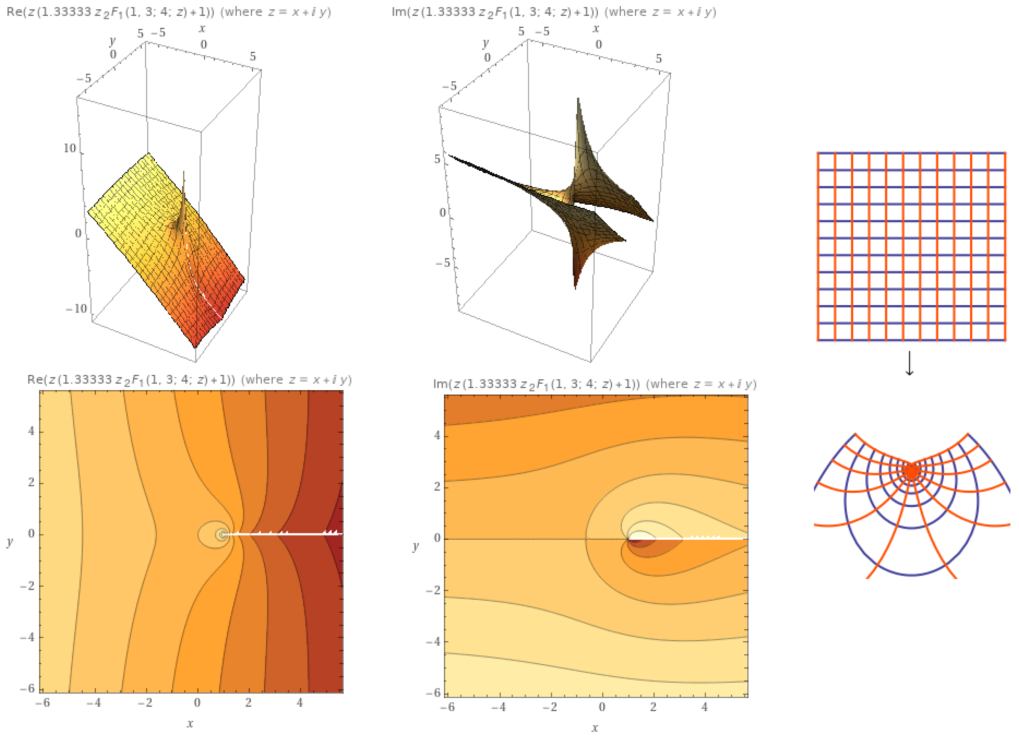
Theorem 6. Consider the class of analytic functions Then, the solution of the differential equation corresponding to this class iswhere represents the hypergeometric function. Proof. Suppose that
Then, it yields the differential equation
where
and
This implies the integral equation
To find the upper solution, we let
Thus, we have the differential equation
Rewrite the above equation as follows:
Multiplying the above equation by the functional
then, we obtain
Hence, it yields solution (
18). □
Example 3. For, and in view of Theorem 6, we have the solution (see Figure 1) 6. Conclusions
The above investigation shows the extension of the ABC-fractional operator in the open unit disk and its generalization by using Jackson calculus. We expressed it in a linear convolution operator acting on a normalized analytic function. A class of analytic functions is studied involving the suggested operator. As an application, we consider the 2D-shallow water differential equation. We discovered its solution in terms of a special function-type hypergeometric function. Moreover, we indicated that the solution is also in the class of normalized analytic functions.
For future works, we suggest modifying the operator acting on different classes of holomorphic functions including the multi-valent, meromorphic and harmonic functions in the open unit disk.
Author Contributions
Conceptualization, R.W.I. and D.B.; methodology, D.B.; formal analysis, R.W.I. All authors have read and agreed to the published version of the manuscript.
Funding
This research received no external funding.
Data Availability Statement
No new data were created or analyzed in this study. Data sharing is not applicable to this article.
Conflicts of Interest
The authors declare no conflict of interest.
References
- Srivastava, H.M.; Kiliçman, A.; Abdulnaby, Z.E.; Ibrahim, R.W. Generalized convolution properties based on the modified Mittag-Leffler function. J. Nonlinear Scien. Appl. 2017, 10, 4284–4294. [Google Scholar] [CrossRef] [Green Version]
- Meshram, C.; Ibrahim, R.W.; Meshram, S.G.; Jamal, S.S.; Imoize, A.L. An efficient authentication with key agreement procedure using Mittag-Leffler-Chebyshev summation chaotic map under the multi-server architecture. J. Supercomput. 2021, 1–22. [Google Scholar] [CrossRef]
- Ibrahim, R.W. Maximize minimum utility function of fractional cloud computing system based on search algorithm utilizing the Mittag-Leffler sum. Int. J. Anal. Appl. 2018, 16, 125–136. [Google Scholar]
- Noreen, S.; Raza, M.; Liu, J.L.; Arif, M. Geometric Properties of Normalized Mittag-Leffler Functions. Symmetry 2019, 11, 45. [Google Scholar] [CrossRef] [Green Version]
- Liu, J.L.; Srivastava, R. A linear operator associated with the Mittag-Leffler function and related conformal mappings. J. Appl. Anal. Comput. 2018, 8, 1886–1892. [Google Scholar]
- Ryapolov, P.A.; Postnikov, E.B. Mittag-Leffler Function as an Approximant to the Concentrated Ferrofluid’s Magnetization Curve. Fractal Fract. 2021, 5, 147. [Google Scholar] [CrossRef]
- Aizinger, V.; Dawson, C. A discontinuous Galerkin method for two-dimensional flow and transport in shallow water. Adv. Water Resour. 2002, 25, 67–84. [Google Scholar] [CrossRef]
- Issakhov, A.; Zhandaulet, Y. Numerical study of dam break waves on movable beds for complex terrain by volume of fluid method. Water Resour. Manag. 2020, 34, 463–480. [Google Scholar] [CrossRef]
- Hauck, M.; Aizinger, V.; Frank, F.; Hajduk, H.; Rupp, A. Enriched Galerkin method for the shallow-water equations. Gem-Int. J. Geomath. 2020, 11, 1–25. [Google Scholar] [CrossRef]
- Miller, S.S.; Mocanu, P.T. Differential Subordinations: Theory and Applications; CRC Press: Boca Raton, FL, USA, 2000. [Google Scholar]
- Srivastava, H.M. Some families of Mittag-Leffler type functions and associated operators of fractional calculus (Survey). TWMS J. Pure Appl. Math. 2016, 7, 123–145. [Google Scholar]
- Atangana, A.; Baleanu, D. New fractional derivatives with nonlocal and non-singular kernel: Theory and application to heat transfer model. arXiv 2016, arXiv:1602.03408. [Google Scholar] [CrossRef] [Green Version]
- Fernandez, A. A complex analysis approach to Atangana-Baleanu fractional calculus. Math. Methods Appl. Sci. 2019, 44, 8070–8087. [Google Scholar] [CrossRef] [Green Version]
- Shukla, A.K.; Prajapati, J.C. On a generalization of Mittag-Leffler function and its properties. J. Math. Anal. Appl. 2007, 336, 797–811. [Google Scholar] [CrossRef] [Green Version]
- Haubold, H.J.; Mathai, A.M.; Saxena, R.K. Mittag-Leffler functions and their applications. J. Appl. Math. 2011, 2011, 298628. [Google Scholar] [CrossRef] [Green Version]
- Salagean, G.S. Subclasses of univalent functions. In Complex Analysis–Fifth Romanian-Finnish Seminar; Springer: Berlin/Heidelberg, Germany, 1983; pp. 362–372. [Google Scholar]
- Jackson, F.H. q-form of Taylor’s theorem. Messenger Math. 1909, 38, 62–64. [Google Scholar]
- Sharma, S.K.; Jain, R. On some properties of generalized q-Mittag Leffler function. Math. Aeterna 2014, 4, 613–619. [Google Scholar]
- Ibrahim, R.W.; Elobaid, R.M.; Obaiys, S.J. A class of quantum Briot-Bouquet differential equations with complex coefficients. Mathematics 2020, 8, 794. [Google Scholar] [CrossRef]
- Ibrahim, R.W.; Elobaid, R.M.; Obaiys, S.J. On subclasses of analytic functions based on a quantum symmetric conformable differential operator with application. Adv. Differ. Equ. 2020, 2020, 325. [Google Scholar] [CrossRef]
- Ibrahim, R.W.; Baleanu, D. On quantum hybrid fractional conformable differential and integral operators in a complex domain. Revista de la Real Academia de Ciencias Exactas, Fisicasy Naturales. Ser. A Mat. 2021, 115, 1–13. [Google Scholar]
- Ibrahim, R.W.; Hadid, S.B.; Momani, S. Generalized Briot-Bouquet differential equation by a quantum difference operator in a complex domain. Int. J. Dyn. Control 2020, 8, 762–771. [Google Scholar] [CrossRef]
- Shanmugam, T.N.; Sivasubramanian, S.; Srivastava, H.M. Differential sandwich theorems for certain subclasses of analytic functions involving multiplier transformations. Integral Transform. Spec. Funct. 2006, 17, 889–899. [Google Scholar] [CrossRef]
- Miller, S.S.; Mocanu, P.T. Subordinants of differential superordinations. Complex Var. 2003, 48, 815–826. [Google Scholar] [CrossRef]
- Guo, D.; Liu, M.-S. On certain subclass of Bazilevic functions. J. Inequal. Pure Appl. Math. 2007, 8, 1–11. [Google Scholar]
- Ruscheweyh, S. Convolutions in Geometric Function Theory. Ph.D. Thesis, Les Presses De L’Universite De Montreal, Montreal, QC, Canada, 1982. [Google Scholar]
| Publisher’s Note: MDPI stays neutral with regard to jurisdictional claims in published maps and institutional affiliations. |
© 2021 by the authors. Licensee MDPI, Basel, Switzerland. This article is an open access article distributed under the terms and conditions of the Creative Commons Attribution (CC BY) license (https://creativecommons.org/licenses/by/4.0/).


