Nanoscale Automated Quantitative Mineralogy: A 200-nm Quantitative Mineralogy Assessment of Fault Gouge Using Mineralogic

Abstract
:
1. Introduction
1.1. Automated Quantitative Mineralogy (AQM)
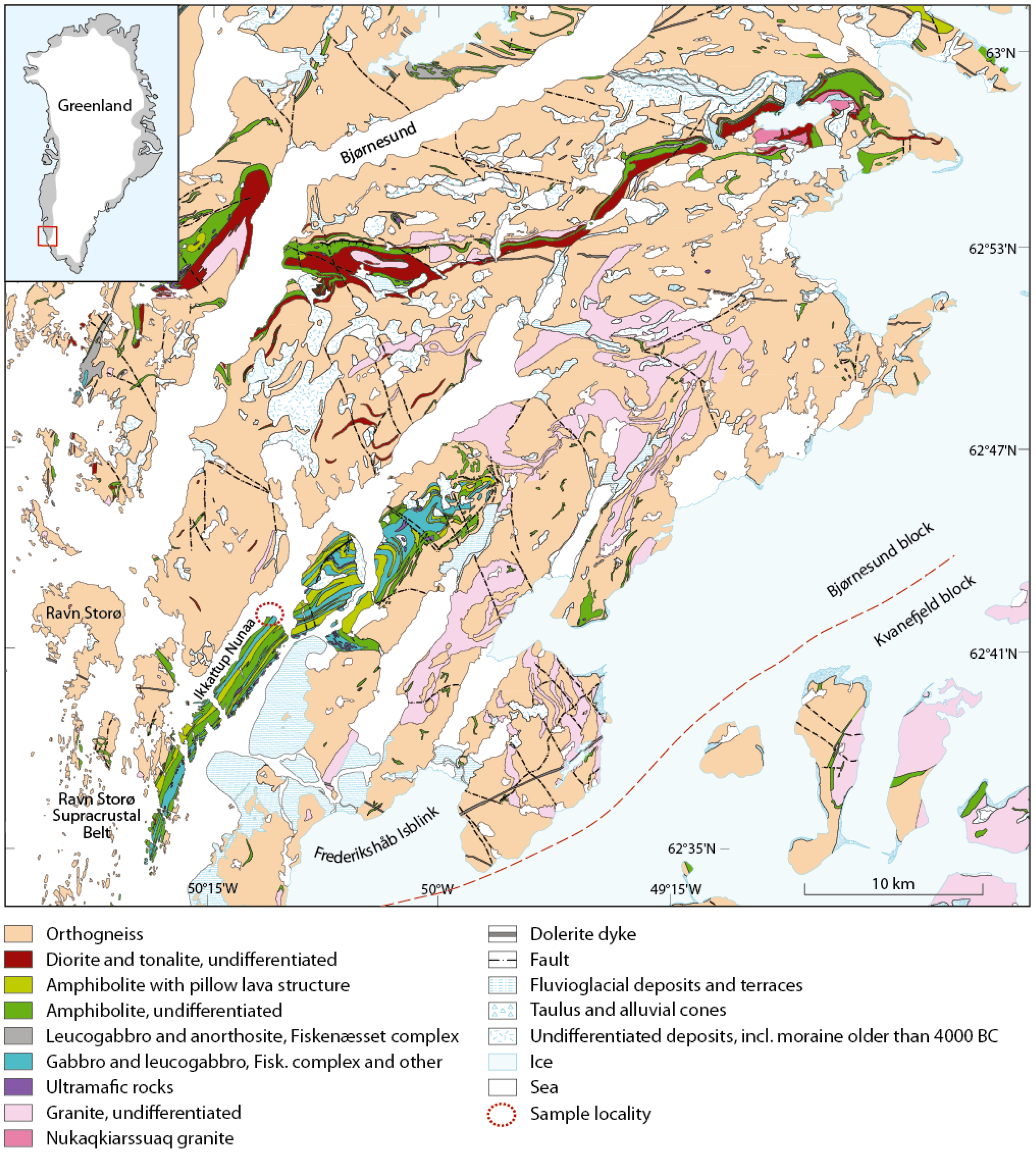
1.2. Geological Background
2. Materials and Methods
3. Results
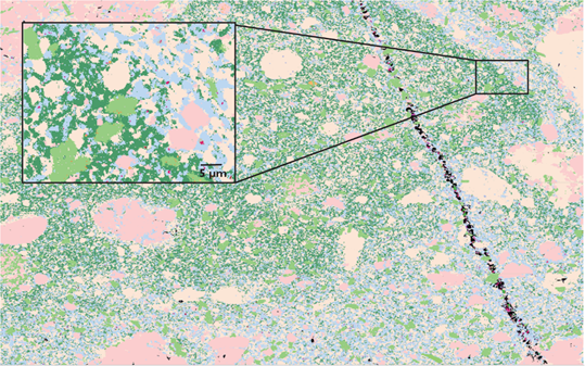
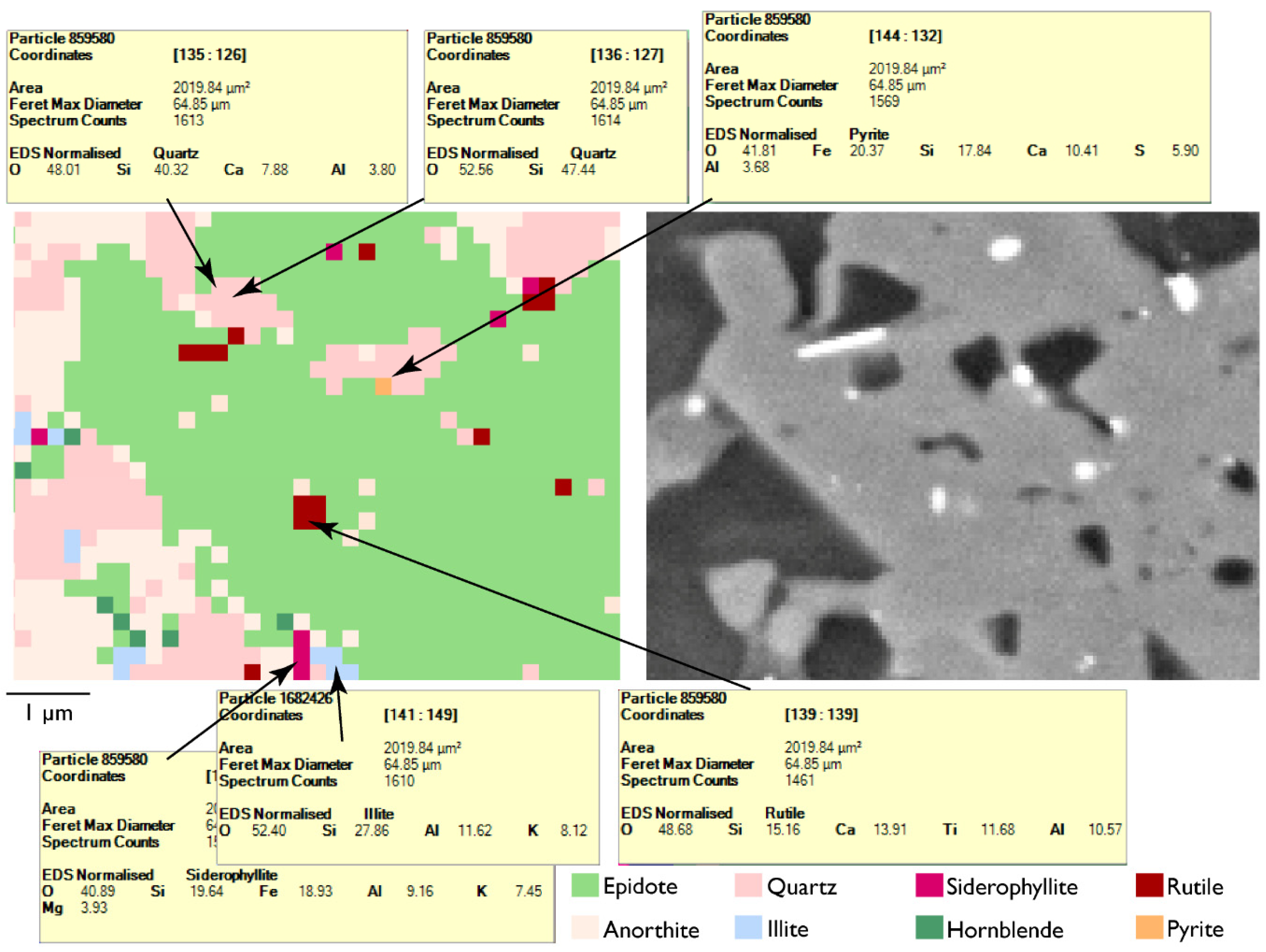
3.1. Mineralogy
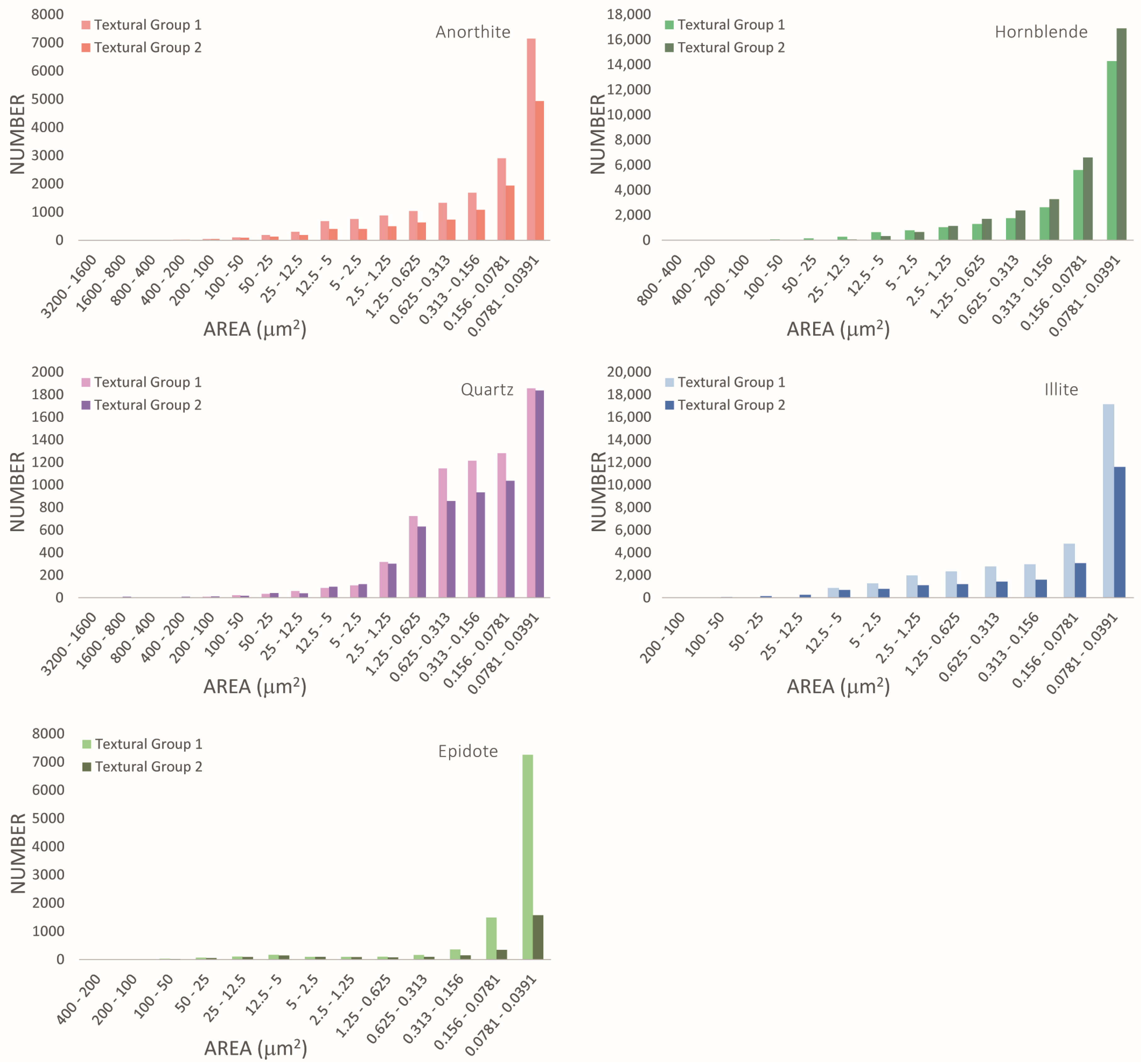
3.2. Grain Size Distributions
4. Implications
5. Conclusions
Author Contributions
Funding
Acknowledgments
Conflicts of Interest
References
- Sutherland, D.N.; Gottlieb, P. Application of automated quantitative mineralogy in mineral processing. Min. Eng. 1991, 4, 753–762. [Google Scholar] [CrossRef]
- Hrtska, T.; Gottlieb, P.; Skála, R.; Breiter, K.; Motl, D. Automated mineralogy and petrology—Applications of Tescan Integrated Mineral Analyzer (TIMA). J. Geosci. 2018, 63, 47–63. [Google Scholar]
- Lotter, N.-O.; Kowal, D.L.; Tuzun, M.A.; Whittaker, P.J.; Kormos, L. Sampling and flotation testing of Sudbury Basin drill core for process mineralogy modelling. Miner. Eng. 2003, 16, 857–864. [Google Scholar] [CrossRef]
- Gottlieb, P.; Wilkie, G.; Sutherland, D.; Ho-Tun, E.; Suthers, S.; Perera, K.; Jenkins, B.; Spencer, S.; Butcher, A.; Rayner, J. Using quantitative electron microscopy for process mineralogy applications. JOM 2000, 52, 24–25. [Google Scholar] [CrossRef]
- Andersen, J.C.Ø.; Rollinson, G.K.; Snook, B.; Herrington, R.; Fairhurst, R.J. Use of QEMSCAN® for the characterization of Ni-rich and Ni-poor goethite in laterite ores. Min. Eng. 2009, 22, 1119–1129. [Google Scholar] [CrossRef]
- Newbury, D.E. Energy-dispersive spectrometry. In Methods in Materials Research; Kaufmann, E.N., Abbaschian, R., Barnes, P.A., Bocarsly, A.B., Chien, C.-L., Dollimore, D., Doyle, B.L., Fultz, B., Goldman, A.I., Gronsky, R., et al., Eds.; John Wiley & Sons: New York, NY, USA, 2000; pp. 11d.1.1–11d.1.25. [Google Scholar]
- Newbury, D.E.; Ritchie, N.W.M. Is Scanning Electron Microscopy/Energy Dispersive X-ray Spectrometry (SEM/EDS) Quantitative? Scanning 2013, 35, 141–168. [Google Scholar] [CrossRef] [PubMed]
- Holwell, D.A.; Adeyemi, Z.; Ward, L.A.; Graham, S.D.; Smith, D.J.; McDonald, I.; Smith, J.W. Low temperature alteration and upgrading of magmatic Ni-Cu-PGE sulfides as a source for hydrothermal Ni and PGE ores: A quantitative approach using automated mineralogy. Ore Geol. Rev. 2017, 91, 718–740. [Google Scholar] [CrossRef]
- Keulen, N.; Malkki, S.N.; Graham, S. Automated quantitative mineralogy applied to metamorphic rocks. Minerals 2019. Submitted this volume. [Google Scholar]
- Goldstein, J.I.; Newbury, D.E.; Michael, J.R.; Ritchie, N.W.M.; Scott, J.-H.J.; Joy, C.C. Scanning Electron Microscopy and X-Ray Microanalysis; Springer: New York, NY, USA, 2017; p. 550. [Google Scholar]
- Keulen, N.; Schumacher, J.C.; Næraa, T.; Kokfelt, T.F.; Schersten, A.; Szilas, K.; van Hinsberg, V.J.; Schlatter, D.M.; Windley, B.F. Meso- and Neoarchaean geological history of the Bjørnesund and Ravns Storø Supracrustal Belts, southern West Greenland: Settings for gold enrichment and corundum formation. Precambrian Res. 2014, 254, 36–58. [Google Scholar] [CrossRef]
- Windley, B.F.; Garde, A.A. Arc-generated blocks with crustal sections in the North Atlantic craton of West Greenland: New mechanisms of crustal growth in the Archaean with modern analogues. Earth Sci. Rev. 2009, 93, 1–30. [Google Scholar] [CrossRef]
- Keulen, N.; Kokfelt, T.F. The Homogenisation Team, 2011. A Seamless, Digital, Internet-Based Geological Map of South-West and Southern West Greenland, 1:100 000, 61°30′–64°. Copenhagen: Geological Survey of Denmark and Greenland. Available online: http://geuskort.geus.dk/gisfarm/svgrl.jsp (accessed on 9 May 2018).
- Keulen, N.; Stünitz, H.; Heilbronner, R. Healing microstructures of experimental and natural fault gouge. J. Geophys. Res. 2008, 113, B06205. [Google Scholar] [CrossRef]
- Hombourger, C.; Outrequin, M. Quantitative Analysis and High-Resolution X-ray Mapping with a Field Emission Electron Microprobe. Microsc. Today 2013, 21, 10–15. [Google Scholar] [CrossRef]
- McSwiggen, P. Characterisation of sub-micrometre features with the FE-EPMA. IOP Conf. Ser. Mater. Sci. Eng. 2014, 55, 012009. [Google Scholar] [CrossRef]
- Fournelle, J.; Cathey, H.; Pinard, P.T.; Richter, S. Low voltage EPMA: Experiments on a new frontier in microanalysis—Analytical lateral resolution. IOP Conf. Ser. Mater. Sci. Eng. 2016, 109, 012003. [Google Scholar] [CrossRef]
- Hovington, P.; Drouin, D.; Gauvin, R. CASINO: A new Monte Carlo Code in C Language for Electron Beam Interaction—Part 1: Description of the program. Scanning 1997, 19, 1–14. [Google Scholar] [CrossRef]
- Drouin, D.; Couture, A.R.; Joly, D.; Tastet, X.; Aimez, V.; Gauvin, R. CASINO V2.42—A fast and Easy-to-use modeling tool for scanning electron microscopy and microanalysis users. Scanning 2007, 29, 92–101. [Google Scholar] [CrossRef]
- Stünitz, H.; Fitzgerald, J.D. Deformation of granitoids at low metamorphic grade. II: Granular flow in albite-rich mylonites. Tectonophysics 1983, 221, 299–324. [Google Scholar]
- Tullis, J.; Yund, R.A. Dynamic recrystallization of feldspar: A mechanism for ductile shear zone formation. Geology 1985, 13, 238–241. [Google Scholar] [CrossRef]
- Velde, B.; Suzuku, T.; Nicot, E. Pressure-temperature of illite-smectite mixed-layer minerals: Niger delta mudstones and other examples. Clays Clay Miner. 1986, 34, 435–441. [Google Scholar] [CrossRef]
- Kristmannsdottir, H. Alteration of Basaltic Rocks by Hydrothermal-Activity at 100–300 °C. Dev. Sedim. 1979, 27, 359–367. [Google Scholar]
- Abd Emola, A.; Charpentier, D.; Buatier, M.; Lanari, P.; Monié, P. Textural-chemical changes and deformation conditions registered by phyllosilictes in a fault zone (Pic de Port Vieux thrust, Pyrenees). Appl. Clay Sci. 2017, 144, 88–103. [Google Scholar] [CrossRef]


| Mineral | Area% | Avg Grain Size (µm) | Grain Size Std Dev (µm) | Average Composition |
|---|---|---|---|---|
| Anorthite | 38.78 | 1.57 | 3.73 | O 40.8; Si 35.62; Al 15.26; Ca 7.29; Fe 0.94; Mg 0.08; K 0.02 |
| Illite | 19.91 | 0.95 | 1.72 | O 37.19; Si 31.84; Al 11.91; Fe 8.64; Ca 4.56; K 3.48; Mg 2.38 |
| Hornblende | 19.86 | 0.85 | 1.84 | O 37.4; Si 31.01; Al 12.71; Fe 9.41; Ca 7.81; Mg 1.46; Ti 0.18; K 0.02 |
| Quartz | 13.27 | 1.11 | 2.62 | Si 54.77; O 43.28; Al 1.95 |
| Epidote | 6.12 | 0.76 | 1.89 | O 36.56; Si 25.6; Ca 16.18; Al 14.49; Fe 7.01; Mg 0.09; Ti 0.07 |
| Siderophyllite | 0.25 | 0.44 | 0.46 | O 34.83; Si 22.99; Fe 19.45; Al 12.26; K 6.23; Mg 4.24 |
| Muscovite | 0.09 | 0.31 | 0.25 | O 50.65; Si 30.4; Al 10.65; K 6.19; Mg 1.52; Na 0.25; Fe 0.18; Ca 0.16 |
| Pyrite | 0.08 | 0.44 | 0.32 | Fe 65.19; S 34.8; Zn 0.01 |
| Apatite | 0.07 | 1.91 | 3.80 | Ca 42.22; O 40.11; P 17.6; Cl 0.07; F 0 |
| Ankerite | 0.06 | 0.32 | 0.27 | O 57.36; Ca 27.14; Fe 12.99; Mg 2.52 |
| Rutile | 0.05 | 0.52 | 0.34 | O 65.7; Ti 34.3 |
| Chamosite | 0.02 | 0.61 | 1.02 | O 33.59; Fe 24.66; Si 22.26; Al 14.33; Mg 5.03; Ca 0.13; K 0.01; Mn 0 |
| K Feldspar | 0.02 | 0.46 | 0.55 | O 37.48; Si 34.62; Al 13.03; K 12.34; Ca 1.74; Fe 0.59; Mg 0.21 |
| Calcite | 0.01 | 0.85 | 0.86 | O 52.63; Ca 44.23; Al 2.42; Fe 0.49; K 0.1; Mg 0.08; S 0.02; Mn 0.02 |
| Area | Average Grain Size | Grain Size Standard Distribution | ||||||||||
|---|---|---|---|---|---|---|---|---|---|---|---|---|
| Mineral | TG1 | TG2 | Absolute Difference | Relative Difference (%) | TG1 | TG2 | Absolute Difference | Relative Difference (%) | TG1 | TG2 | Absolute Difference | Relative Difference (%) |
| Anorthite | 40.68 | 39.92 | 0.76 | 1.89 | 1.55 | 1.62 | −0.07 | −4.50 | 3.59 | 4.21 | −0.62 | −15.94 |
| Illite | 15.14 | 23.46 | −8.32 | −43.09 | 0.87 | 1.08 | −0.22 | −22.26 | 1.26 | 2.23 | −0.98 | −55.94 |
| Quartz | 9.59 | 18.86 | −9.27 | −65.17 | 1.07 | 1.21 | −0.15 | −12.73 | 2.26 | 3.27 | −1.01 | −36.69 |
| Hornblende | 26.36 | 10.31 | 16.05 | 87.54 | 1.02 | 0.71 | 0.31 | 36.15 | 2.36 | 1.09 | 1.28 | 74.06 |
| Epidote | 6.23 | 5.49 | 0.74 | 12.62 | 0.61 | 1.40 | −0.79 | −78.44 | 1.59 | 2.71 | −1.12 | −52.18 |
| Siderophyllite | 0.20 | 0.29 | −0.08 | −34.21 | 0.41 | 0.47 | −0.06 | −14.16 | 0.46 | 0.50 | −0.04 | −7.59 |
| Muscovite | 0.07 | 0.12 | −0.05 | −54.68 | 0.32 | 0.31 | 0.02 | 4.92 | 0.27 | 0.25 | 0.02 | 7.87 |
| Apatite | 0.04 | 0.09 | −0.06 | −88.82 | 1.99 | 1.83 | 0.16 | 8.47 | 2.81 | 4.16 | −1.35 | −38.59 |
| Ankerite | 0.06 | 0.06 | 0.00 | −0.89 | 0.32 | 0.33 | 0.00 | −1.10 | 0.27 | 0.28 | −0.01 | −4.21 |
| Pyrite | 0.09 | 0.06 | 0.03 | 41.86 | 0.41 | 0.48 | −0.08 | −16.87 | 0.34 | 0.26 | 0.08 | 25.95 |
| Rutile | 0.05 | 0.05 | 0.00 | −9.21 | 0.50 | 0.55 | −0.05 | −9.64 | 0.34 | 0.34 | 0.00 | −0.12 |
| Chamosite | 0.01 | 0.04 | −0.03 | −127.75 | 0.41 | 0.76 | −0.35 | −60.31 | 0.68 | 1.17 | −0.49 | −52.38 |
| K Feldspar | 0.02 | 0.01 | 0.00 | 0.51 | 0.54 | 0.40 | 0.14 | 29.69 | 0.77 | 0.37 | 0.41 | 71.40 |
| Calcite | 0.01 | 0.01 | 0.00 | −20.93 | 0.75 | 0.81 | −0.07 | −8.41 | 0.71 | 0.78 | −0.07 | −9.25 |
© 2019 by the authors. Licensee MDPI, Basel, Switzerland. This article is an open access article distributed under the terms and conditions of the Creative Commons Attribution (CC BY) license (http://creativecommons.org/licenses/by/4.0/).
Share and Cite
Graham, S.; Keulen, N. Nanoscale Automated Quantitative Mineralogy: A 200-nm Quantitative Mineralogy Assessment of Fault Gouge Using Mineralogic. Minerals 2019, 9, 665. https://doi.org/10.3390/min9110665
Graham S, Keulen N. Nanoscale Automated Quantitative Mineralogy: A 200-nm Quantitative Mineralogy Assessment of Fault Gouge Using Mineralogic. Minerals. 2019; 9(11):665. https://doi.org/10.3390/min9110665
Chicago/Turabian StyleGraham, Shaun, and Nynke Keulen. 2019. "Nanoscale Automated Quantitative Mineralogy: A 200-nm Quantitative Mineralogy Assessment of Fault Gouge Using Mineralogic" Minerals 9, no. 11: 665. https://doi.org/10.3390/min9110665
APA StyleGraham, S., & Keulen, N. (2019). Nanoscale Automated Quantitative Mineralogy: A 200-nm Quantitative Mineralogy Assessment of Fault Gouge Using Mineralogic. Minerals, 9(11), 665. https://doi.org/10.3390/min9110665