Article

Mineralogical Imaging for Characterization of the Per Geijer Apatite Iron Ores in the Kiruna District, Northern Sweden: A Comparative Study of Mineral Liberation Analysis and Raman Imaging

1
Division of Economic Geology and Petrology, Technische Universität Bergakademie Freiberg, Akademiestraße 6, 09599 Freiberg, Germany
2
Chair of Bioanalytical Chemistry, Dresden University of Technology, 01069 Dresden, Germany
3
Luossavaara Kiirunavaara AB (publ.), 98186 Kiruna, Sweden
*
Author to whom correspondence should be addressed.
Minerals 2019, 9(9), 544; https://doi.org/10.3390/min9090544
Submission received: 14 August 2019 / Revised: 5 September 2019 / Accepted: 6 September 2019 / Published: 10 September 2019

Abstract

:
The Per Geijer iron oxide apatite deposits are important potential future resources for Luossavaara-Kiirunavaara Aktiebolag (LKAB) which has been continuously mining magnetite/hematite ores in northern Sweden for over 125 years. Reliable and quantitative characterization of the mineralization is required as these ores inherit complex mineralogical and textural features. Scanning electron microscopy-based analyses software, such as mineral liberation analyzer (MLA) provide significant, time-efficient analyses. Similar elemental compositions of Fe-oxides and, therefore, almost identical backscattered electron (BSE) intensities complicate their discrimination. In this study, MLA and Raman imaging are compared to acquire mineralogical data for better characterization of magnetite and hematite-bearing ores. The different approaches demonstrate advantages and disadvantages in classification, imaging, discrimination of iron oxides, and time consumption of measurement and processing. The obtained precise mineralogical information improves the characterization of ore types and will benefit future processing strategies for this complex mineralization.

1. Introduction

The mineralogical characterization of ore deposits using scanning electron microscopy (SEM)-based automated mineralogy systems such as mineral liberation analyzer (MLA) or QEMSCAN® are of major importance for mineral processing. Declining ore grades, the reconnaissance of new targets, and demands for improved energy efficiency require fast, reliable, and high-quality information on mineral resources. Highly variable and complex mineralogy affects mineral processing and extractive metallurgy, as has been shown by authors in the past [1,2,3,4,5,6]. Collecting quantitative data of mineral distributions, associations and textures are one of its key abilities. Using this technique, information gained by traditional bulk mineralogical analysis, chemical assay, and optical microscopy can be supported and expanded. Automated mineralogy is widely used in the mining business as it allows rapid identification and characterization of key minerals in ore and rock samples. Furthermore, it can be applied to all sorts of different mineral deposit types [1,7,8,9,10,11]. Mineral liberation analysis (MLA) software is one of the widely applied SEM-based applications offering a rapid quantitative characterization of mineral species and their relations in polished samples [12]. It is commonly used in conjunction with other micro-compositional or microstructural techniques such as electron-probe microanalyses (EPMA) or X-ray diffraction (XRD). However, SEM-based techniques cannot precisely distinguish mineral polymorphs (e.g., rutile-anatase-brookite) or discriminate between minerals having a similar elemental composition (e.g., magnetite and hematite). Especially the discrimination of magnetite and hematite becomes an important factor in future processing stages at the Luossavaara-Kiirunavaara Aktiebolag (LKAB) enterprise. Almost pure magnetite mineralization is only prevalent in the Kiirunavaara deposit. Increasing hematite contents in the other deposits in the Kiruna district (Malmberget and Leveäniemi), and most predominantly in Per Geijer will significantly influence the beneficiation and pelletizing process. In order to sustain efficient comminution and magnetic separation processes evaluation by automated mineralogy or similar methods will add significant value in the future.
The effect that similar average atomic numbers result in similar BSE intensities (BSE grey values) requires modification of the MLA technique, especially in the data processing stage. A technique for distinguishing between hematite and magnetite by MLA has been established by Figueroa et al. [13]. However, stable beam currents and even sample surfaces are obligatory for maintaining constant BSE grey values. As this often proves problematic, there is demand for additional analytic solutions.
In this study, Raman imaging is used as an alternative tool to highlight advantages and disadvantages of both methods with the focus on magnetite-hematite mineralization of the Per Geijer iron ore deposits close to the well-known Kiirunavaara deposit. This comparative approach for ore characterization provides detailed information by mapping mineral distributions of a potential new iron ore resource.

2. Geology of the Per Geijer Deposits

The iron oxide apatite ores (IOA) in the Kiruna area are hosted by the Svecofennian Kiirunavaara Group. Svecofennian rocks are represented by volcanic and sedimentary units generated by reworking of older crust and subduction and accretion of several volcanic arc complexes [14,15,16,17]. Three formations account for that group: (1) Hopukka Formation, (2) Luossavaara Formation, and (3) Matojärvi Formation. The giant Kiirunavaara ore body with pre-mining resources of more than 2000 Mt [18], is a massive tabular almost purely magnetite body with generally low phosphorus content. The smaller, magnetite-rich Luossavaara deposit north of Kiirunavaara is situated in the same stratigraphy. Closely associated with the east and northeast reside the Per Geijer orebodies at the stratigraphically upper contact of the Luossavaara Formation or within the lower part of the Matojärvi Formation [19]. These deposits are located north of the town of Kiruna and consist of five orebodies that have been mined in intervals during the 20th century as open pits. The Nukutus, Henry, and Rektorn mineralization occur stratigraphically at the upper contact of the Luossavaara Formation, while the Haukivaara and Lappmalmen deposits, at least partly, are located within the overlying Matojärvi Formation. Lappmalmen is a blind and, so far, unexploited ore body only known from exploration drilling. The ores exhibit large variations in texture, mineral composition, and relation to wall rocks [18]. Depending on the orebody and the vertical position of the mineralization in the deposit, magnetite and hematite occur in varying textures and proportions leading to different ore types (e.g., hematite-dominated, magnetite-dominated, magnetite/hematite-mixed), as proposed by [20]. Generally, hematite occurs together with magnetite often replacing it, especially close to the upper part of the deposit. The overall phosphorus content is high and occurs as apatite. Other main gangue minerals are carbonate and quartz. The Per Geijer deposits have an average composition of 40–50% Fe and 3–5% P but higher and lower iron and phosphorus contents can locally occur.

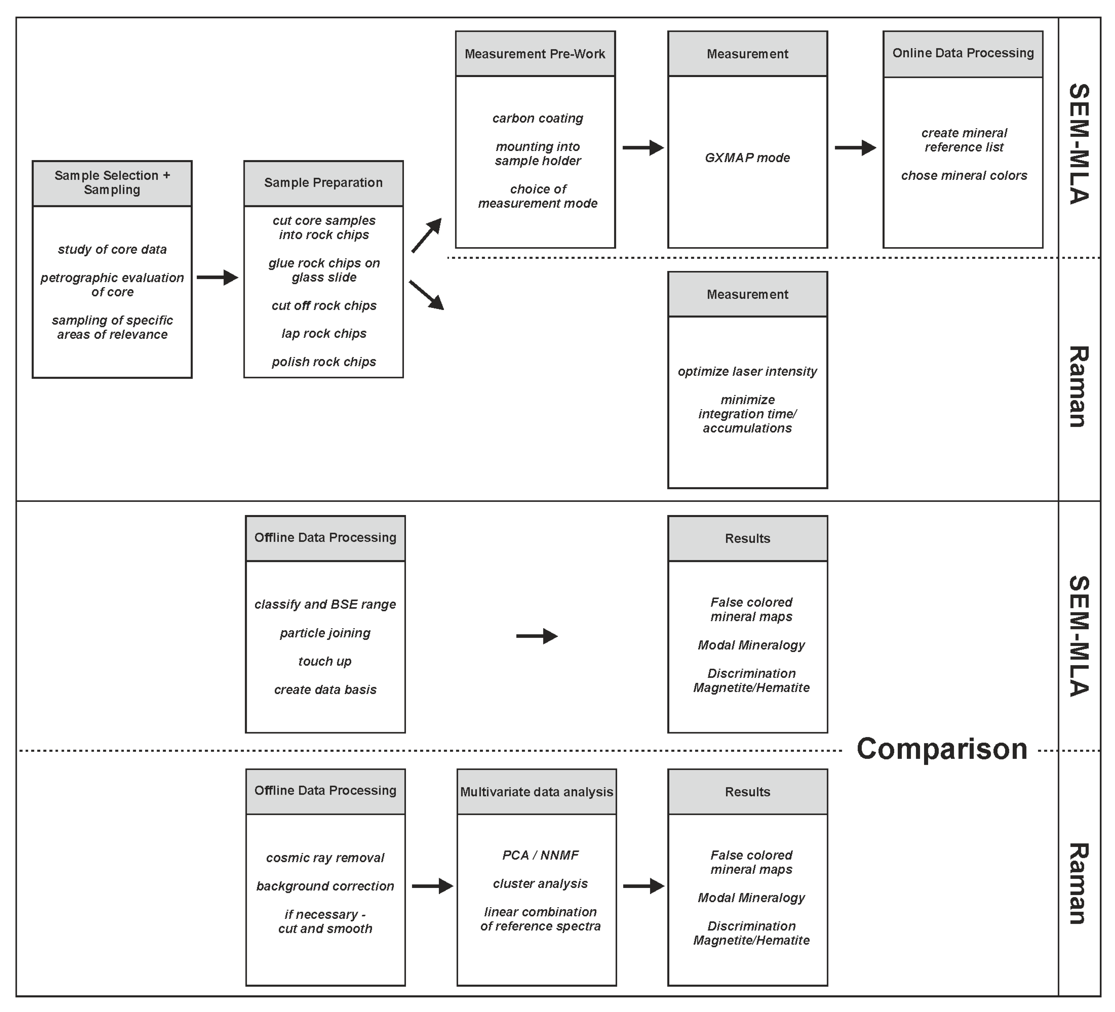
3. Materials and Methods

3.1. Samples and Preparation

Sixty-five samples were selected from drill cores representing all five Per Geijer ore bodies after specific pre-defined ore type sections and macroscopic petrographic evaluation. For this study, 18 polished thin sections were prepared by the preparation laboratory of the Helmholtz Institute Freiberg for Resource Technology. Sample HA-81155-2 was selected for comparative SEM-MLA and Raman measurements because of the occurrence of magnetite, hematite, and Ti-bearing hematite in satisfying abundances.

3.2. Scanning Electron Microscope (SEM) and Mineral Liberation Analyzer (MLA)

Samples were studied with the scanning electron microscope (SEM) including mineral liberation analyzer (MLA) (FEI, Brisbane, Australia) software on a Quanta 650 FEG-MLA650F (FEI©, Brno, Czech Republic). The analyses were carried out at the geometallurgical laboratory of the Department of Mineralogy at TU Bergakademie Freiberg, Germany. Energy-dispersive X-ray spectroscopy (EDS) was performed with two Bruker Nano Dual X-Flash 5030 detectors (Bruker, Berlin, Germany), using an accelerating voltage of 25 kV and a working distance of 12 mm. The workflow of the SEM-MLA analysis described in the following sections is shown in Figure 1.

3.2.1. Measurement Mode and Setup

The grain-based X-ray mapping (GXMAP) mode was selected for this study. The GXMAP technique analyses selected grains (in this case, the whole thin section) with a closely spaced grid of X-ray measurements resulting in false-colored mineral maps [12,21]. Here, the whole sample was continuously mapped with an EDS analysis every 12 μm (slower mapping) or 36 μm (faster mapping). In both measurements, the frame resolution was 500 × 500 pixel with a magnification of either 3 or 2 μm/pixel, respectively. Based on backscattered images, the minerals were first separated according to their grey values and then mapped in a definite grid of EDS analysis. The basic setup included the definition of a BSE grey value range (BSE trigger). As element contents are responsible for the BSE contrast, chemically similar minerals have identical BSE grey levels. Thus, for hematite and magnetite classification, reference BSE values had to be manually defined. Furthermore, they were compared with optical reflected light images of the sample in which the two iron oxides have characteristic reflection properties. The details of the SEM image acquisition are listed in Table 1. A detailed description of the functionality of MLA and the measuring modes can be found in the literature [12,22,23,24].

3.2.2. Mineral Reference List

A preliminary mineral reference list was generated by collecting mineral standards manually. Chemical compositions were obtained with the Bruker Esprit 1.9 software (Bruker, Berlin, Germany), mineral names, and formulae, as well as physical properties (e.g., density), were added.

3.2.3. Online Data Processing

The preliminary mineral list had to be adjusted after first classification due to larger unknowns. Unknowns are detected when the comparison between the spectra of the mineral reference list and the measured X-ray spectra fails. This error in consistency occurs when the limits of a spectrum matching threshold (80%) and/or a low count limit (800) exceed the predetermined values. Thus, an assignation to a suitable mineral phase was not possible. However, some unknowns can be the result of mixed spectra of two different phases.

3.2.4. Offline Data Processing

For off-line image and data processing collected X-ray spectra were classified. As for online data processing, comparison with the spectra of the mineral reference list is necessary. Therefore, the spectrum matching threshold and low count limit were set to 80% and 800 counts, respectively. However, the X-ray spectra and the BSE grey level of the different iron oxides (e.g., hematite and magnetite) are very similar. Consequently, the results from MLA were checked against the results from optical microscopy and manual correction was applied. For most samples, BSE grey value ranges were set at 150 to 190 for hematite and 191 to 250 for magnetite. These values were checked for every sample after classification and adjusted, if necessary. However, single frames in some samples yielded wrong classification of magnetite and hematite based on local BSE grey value variations. Manual correction was obtained by using the edit selected particles mode. By re-defining wrongly classified areas manually, the validity for the samples was improved.
To remove small unknowns and other noise from the image, the touch-up tool was used. All unknowns with a size smaller than 50 pixels were turned into the containing host (unknown to any host), which mainly affected pixels with mixed spectra. The remaining unknowns generated by holes and brackets of the thin section holder were turned into background (size < 2,000,000 pixels). Minerals, which feature a pixel size smaller than 50 or 70 that are located in another mineral, were transformed to the containing host mineral (mineral to any host). Finally, databases were created comprising information about modal mineralogy, mineral associations, as well as grain properties. For this study, only information of the modal mineral abundance was taken into account.

3.3. Raman Spectroscopy and Imaging

Raman maps were collected using an alpha300 M+ Raman Microscope System (WITec GmbH, Ulm, Germany) or an inVia Qontor Raman Confocal Microscope (Renishaw, Pliezhausen, Germany). The workflow of the Raman analysis described in the following sections is shown in Figure 1.

3.3.1. Measurement Mode and Setup

The measurements were carried out at Papiertechnische Stiftung (PTS) Heidenau and Center for Molecular Bioengineering at TU Dresden (BCUBE). Both systems were equipped with an upright microscope using a 532 nm laser excitation and a Charge Coupled Device (CCD) detector with 1024 pixel. The Renishaw system was used with a 100× objective (Leica Objective N plan EPI 100×/NA 0.85) using 10% laser power (corresponding to approximately 5 mW) and a 1800 gr/mm grating (spectral range: 60–1837 cm−1). The Raman map of Figure 2 (2.127 cm × 2.232 cm) was collected with 30 µm step size and 275 ms exposure time using the Renishaw system.
The WITec confocal Raman system is based on a Zeiss microscope and was used with a 100× objective (Zeiss EC Epiplan NA 0.9) using 20 mW laser power and a 600 gr/mm grating (spectral range: −123–3777 cm−1). The Raman maps of Figure 3 were collected using the WITec system. The overview map (2.38 cm × 1.3 mm) was collected with 12 µm step size, the detailed map with 1 µm step size (160 µm × 120 µm). In both cases, spectra were collected using 200 ms exposure time.
Before measurement, we optimized spectral acquisition parameters (especially laser power). Due to the large mapping areas (up to 2 cm × 2 cm), we decided to use the highest laser power while reducing exposure time as much as possible to achieve a high mapping speed. We started with point measurements on all minerals (acquisition time: 0.2 s) using increasing laser power to check for thermal decomposition or oxidation. This way, the maximum laser power for each mineral can be determined. In our samples, sulfides were found to be the most sensitive to laser damage resulting in significant visible and spectroscopical changes. The most sensitive minerals determined the laser power that was used. We did not observe any changes in the spectra of magnetite and hematite. In comparison, the literature reporting on hematite transformation [25], used exposure times from at least several seconds up to several minutes (10 s–5 min). Samples were checked for oxidation effects after measurements with optical reflected light microscopy.

3.3.2. Mineral Reference List

Reference spectra were collected either by spot measurements, isolated by non-negative matrix factorization (NMF), or extracted by averaging mineral-specific areas of Raman maps based on the EDS maps obtained for MLA. Before linear combination, the spectra were background-corrected and normalized. All reference spectra can be found in the Supporting Information (Figure S1).

3.3.3. Offline Data Processing-Data Preprocessing

Spectral datasets were imported into the in-house SpectralImaging software (TU Dresden, Dresden, Germany) on the basis of Matlab provided and developed by Matthias Finger ([email protected]). First, cosmic ray removal was performed to eliminate spikes. Spectral datasets were typically cut to a wavelength of 100–1900 cm−1 where significant spectral differences were found. Baseline correction was performed by asymmetric least squares correction (smoothness 5, asymmetry 2). If necessary, smoothing (Savitzky-Golay, seven points, degree 2) was applied.

3.3.4. Offline Data Processing-Multivariate Analysis

Multivariate analysis was used to identify the number of principal components and to image their distribution. We used two data analyses methods, principal component analysis (PCA) and non-negative matrix factorization (NMF). Both techniques were conducted using the above-mentioned in-house SpectralImaging software based on Matlab.
PCA and NMF are both unsupervised statistical methods to reduce the dimensionality of large datasets. Using PCA, original variables of the dataset are summarized in new variables, the so-called principal components. These components are calculated as the solution of an eigenvalue problem responsible for the whole variance of the data set. As a result, PCA weights a set of principal components with positive and negative values to represent the full spectral information.
NMF is similar to PCA but the weights and factors are constrained to be positive. Therefore, it is well-suited to represent data with non-negative features. We found that the resulting spectral factors are easier to inspect. That is why, if necessary, non-negative matrix factorization (NMF) was used to extract spectral signatures of individual minerals from the total set. To validate these unsupervised methods, a supervised linear combination approach was used to map the distribution of selected components. All maps shown were prepared using linear combination of a set of measured reference spectra (see above).

4. Results

The following results are presented as comparison and verification of SEM-MLA and Raman mapping. Emphasis is given on imaging, discrimination of magnetite and hematite and modal mineralogy in area % with respect to the time demands for measurements and processing.

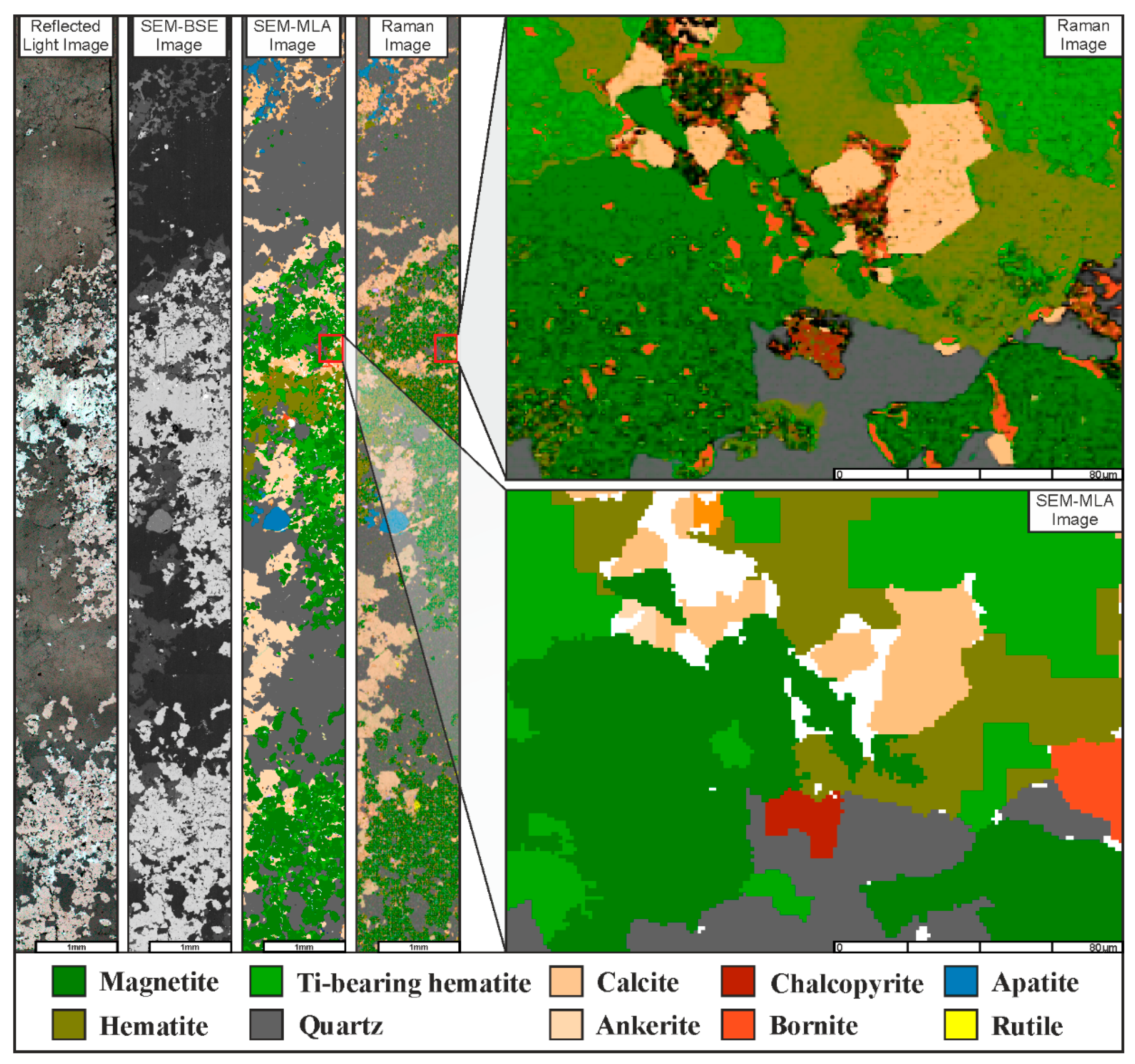
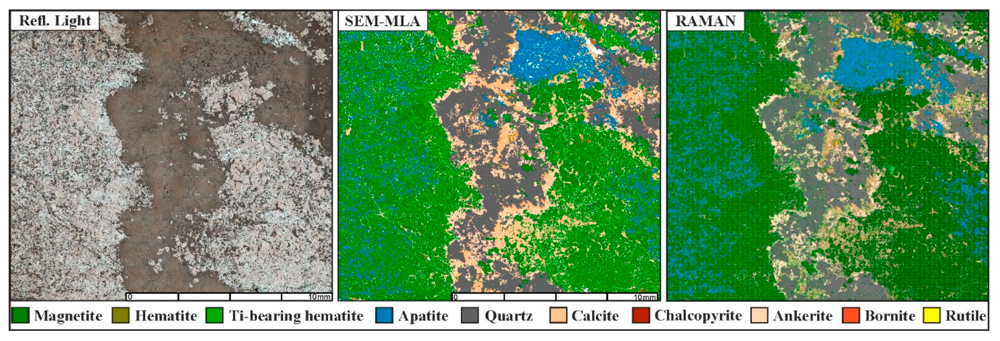
4.1. Classification and Imaging

The mineral distribution maps of both classifications (SEM-MLA and Raman) correspond well with the thin section of the reflected light photograph (Figure 2). Both methods recognized the present minerals. The classification with MLA was manually adjusted with a BSE grey level range from 150 to 190 for hematite and 191 to 250 for magnetite. Mineral boundaries are pre-defined based on the BSE grey values with the SEM-MLA. This function is not yet available for Raman imaging resulting in a rasterized resolution. General features, textures of the sample material and the abundance and location of important minerals are visible with both methods.

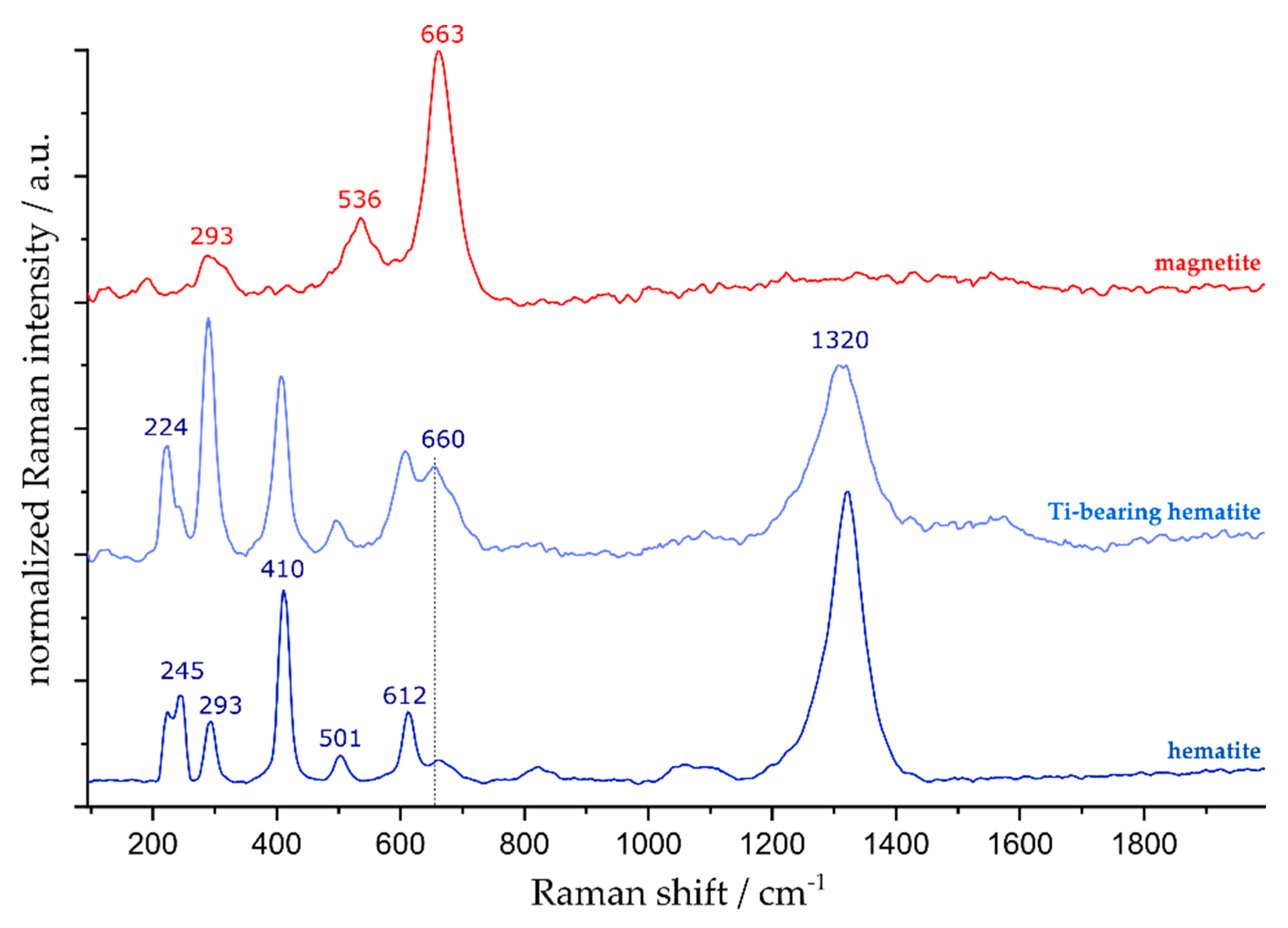
4.2. Discrimination of Magnetite and Hematite

In the reflected light image of the polished sample of apatite iron ore, magnetite, hematite, and gangue minerals (mostly apatite, carbonates, and silicates) can be seen (Figure 3). In SEM-based backscattered electron images, iron oxides are hardly distinguishable from each other due to similar BSE grey values. The processed false-colored mineral maps from MLA and Raman show all present phases. However, the precise discrimination of magnetite and hematite varies with both techniques. A smaller area (see the red square in Figure 3) was selected for high-resolution Raman mapping. Six minerals were spectrally identified within this smaller area, corresponding to magnetite, Ti-free hematite, Ti-bearing hematite, quartz, ankerite, bornite, and chalcopyrite. The different Raman spectra for hematite were assigned to Ti-bearing hematite by EDS data.

4.3. Modal Mineralogy

The modal mineralogy can be extracted in the Dataview software for SEM-MLA measurements. Raman does not commonly offer this data analysis feature as an in-built tool. However, quantification of phase abundances is possible based on the number of pixels identified for each phase in relation to the total number of pixels in the scanned area.
The modal mineralogy of the major and minor components obtained for the area displayed in Figure 2 shows similar results between the slow and the fast SEM-MLA and Raman measurements (Table 2). However, magnetite occurs in higher modal abundance in the measurement with lower step size (35.54 area %) compared to the fast measurement (33.62 area %) and Raman (34.9 area %). Contrary, the modal mineralogy of hematite and Ti-bearing hematite is elevated in the fast GXMAP but lower in Raman (Table 2). Quartz, apatite, and ankerite show slightly lower values compared to SEM-MLA. The modal mineralogy of calcite is in the range of ± 0.2 area % for all measurements.

4.4. Time Constraints

For this study, SEM-based MLA measurements were performed with two different resolutions and step sizes on the same sample in addition to Raman mapping.

4.4.1. Measurement Time

The measurement time for fast GXMAP mapping with a resolution of 500 × 500 pixels and a step size of 36 µm was 6 h. Mapping with a step size of 12 µm and the same resolution took 12 h. The identical area of the same sample measured with Raman was the most time-intensive with 42 h using a step size of 30 µm. The measurement time of the detailed Raman map (Figure 3) took 1 h using a step size of 1 µm.

4.4.2. Data Processing Time

The processing time is dependent on many variables, including the operator in charge, technical equipment, e.g., computational power, software requirements, and functions. In SEM-MLA data processing of faster measurements using larger step sizes resulted in more unknowns and misidentification of phases. In this case, additional processing time was required due to manual correction of the sample set.
Data processing in Raman imaging depends strongly on the signal-to-noise ratio of the acquired spectra. Since processing is done mainly offline after data acquisition, it is crucial to ensure the best acquisition parameters (e.g., laser power, exposure time) before measurement. To discriminate similar minerals (e.g., Ti-bearing and Ti-poor hematite) longer acquisition times are recommended.

5. Discussion

The presented results and images of SEM-MLA and Raman measurements of magnetite and hematite-bearing ores from apatite iron oxide deposits in the Kiruna area depend, in both cases, mainly on the correct classification of the present minerals. For SEM-MLA, a comprehensive mineral database containing all present minerals that are correctly distinguished by their chemical information is inevitable. Raman imaging does not necessarily require any preexisting knowledge about the existing minerals. Therefore, online data processing is not necessary and data analysis happens solely offline after data acquisition, e.g., using unsupervised multivariate data analysis to identify different minerals.
When it comes to mineral classification, Raman shows some major advantages, especially in the discrimination of magnetite and hematite due to their distinct Raman spectral signatures [25,26,27,28,29,30]. A diagnostic Raman peak for magnetite is 663 cm−1 (T2g), whereas hematite is dominated by strong peaks at 293 (Eg), 410 (Eg), 615 (Eg) and 1320 cm−1 (Figure 4). In comparison, Figueroa et al. [13] showed that using the SEM-based MLA method discrimination of magnetite and hematite is possible but needs significant adjustments prior to and during measurements. It was stated, that measurement times did not increase significantly but the process of time-consuming offline modification and the effect of fluctuations in beam current was neglected. The ability of Raman spectroscopy to intrinsically discriminate clearly between magnetite and hematite shows great potential for the characterization of iron oxide deposits. However, it needs to be noted that Fe(II)-containing minerals can be easily converted into Fe(III)-oxides like hematite by high laser powers [25,29,30]. In order to avoid conversion, it is crucial to optimize spectral acquisition parameters prior to mapping (see experimental details).
Another great advantage of Raman spectroscopy is its ability to not only identify, but also quantify incorporated foreign elements. Substitution of iron with aluminum [31,32,33], manganese/chromium [34,35], or titanium [36] results in a shift of Raman peak positions due to differences in mass. In a similar manner, carbonates show changes in peak location and shape depending on the amount of magnesium, iron, and manganese replacing calcium [37,38,39,40]. Ti-bearing hematite was classified by both methods because of the incorporation of ca. 3 wt % Ti. In Raman, we observed a change in the peak intensity at 295 cm−1 and 660 cm−1 (LO Eu) and an increased peak width, especially at 660 cm−1 and 1320 cm−1. A shift to higher wavenumbers, as described by Varshney et al. [36] was not observed most likely due to lack of spectral resolution. The IR-active Eu (LO) at 660 cm−1 is theoretically not allowed (Raman-inactive). The intensity increase at about 660 cm−1 is a common indication for the incorporation of foreign elements. It becomes Raman-active due to structural disorder induced by surface defects or stress [34,35,36].
Please note that Raman imaging can be compromised by fluorescence excited by the laser source. The use of different laser wavelengths, bleaching, or fluorescence correction algorithms can efficiently counter the possible fluorescence of geological samples. If necessary, fluorescent areas can also be visualized using the Raman system.
Raman spectroscopy offers a variety of additional possibilities to characterize inorganic materials in terms of polymorphism, crystal orientation, crystallinity, phase, stress, and strain [41,42]. The combination of the strong and distinct Raman signatures with its nondestructive nature makes Raman spectroscopy a powerful tool for fine-scale identification and characterization of iron oxides.
A summary of the pros and cons of SEM-MLA and Raman imaging is given in Table 3.
Quantification of the mineral abundance is well established using the MLA software (FEI, Brisbane, Australia) [12]. For Raman imaging, quantification using a similar algorithm as described by Fandrich et al. [12] and FEI [21], needs to be implemented for geological applications. For this reason, we decided to compare area % in Table 2, which are easily accessible by both methods. For mineral quantification of the Raman map, we relied solely on the results of linear combination of reference spectra, not taking into account any microscopic data. The results also rely on color thresholds set in the SpectralImaging software. Therefore, it should be noted that the error of the Raman quantification method described here is larger than that of MLA quantification. Nevertheless, both methods reveal similar quantitative analyses of mineral abundance in the range of 1.5% with the exception of Ti-bearing hematite. The discrepancy of >3% is assumed to be caused by the fact that Raman relies on a fixed mapping grid neglecting mineral boundaries visible in the BSE image. Therefore, in some areas the step size of 30 µm is too big to resolve fine structures smaller than 30 µm size. Furthermore, the increased Raman intensity at 660 cm−1 for Ti-bearing hematite could, at least partially, result in a misassignment of magnetite using the linear combination approach.
Another important criterion for institutions and companies working on iron ores is the cost of analysis when making feasible assumptions according to improved characterization and extraction of the ore mineral. In purchase and maintenance, the financial advantage is on the Raman side, as the acquisition of an SEM-MLA (~800.000€) is roughly three times higher than a Raman imaging device including software (~250.000€). Furthermore, operating an SEM requires high vacuum pumps and nitrogen supply. Both techniques require a skilled operator to efficiently adjust measurements and they should be operated in an air-conditioned laboratory. In this study, the analyses were conducted on prepared thin sections for both methods. However, the advantage of Raman on the cost side is further supported by the fact that no sample preparation is needed, whereas SEM-MLA requires preparation and carbon coating of the samples.
Taking into account the limits and potentials of both methods, it is essential to define the right questions to a problem in order to find the most suitable analytical solution. Samples that contain very fine-grained aggregates or minerals that have fine intergrowths may need to be resolved in higher resolution. These detailed maps with a spot size in nm range (up to around half the laser wavelength) are one of the major advantages of the Raman technique, whereas the SEM is limited to µm range (~1 µm) even with the best operating conditions. It should be noted that, with higher resolution and smaller spot, size measurements become more time-consuming. In this study, Raman measurements on the same sample area with the same spot size took at least 10 times longer than MLA mapping, thus they are not nearly as time-efficient. Although Ramanaidou and Wells [43], suggested Raman spectroscopy as a potential method for large volume or bulk analysis, this seems not applicable with stationary Raman spectroscopes at this stage. Transportable Raman devices may offer fast field analysis by point measurements, but the loss of spectral information due to the downsized equipment needs to be compensated. Future instrumental research and development may lead to Raman spectroscopy and imaging as the first order application in process mineralogical analysis of iron ore. However, solely imaging will not solve the need for precise characterization of these complex ores, thus parameters, such as mineral liberation, association or locking, especially from processed ore, need to be extracted. Raman manufacturers start to offer software solutions for particle analysis, e.g., ParticleScout (WITec GmbH, Ulm, Germany), applicable to large sample areas typical for geosciences. The authors of this study are currently working on the development of these functions too, to further enhance the application of Raman imaging as a modern tool for analysis, especially for iron ore.

6. Conclusions

This study has demonstrated the potential of both SEM- and Raman-based mineralogical imaging for the characterization of iron oxide apatite deposits (IOA). In polished sections of IOA, magnetite, hematite, apatite, carbonates, and silicates were easily detected and mapped. The discrimination of magnetite and hematite, however, is strongly dependent on operating conditions in SEM-MLA. Raman imaging shows a major advantage due to distinct Raman spectra that enable in situ identification. Raman spectroscopy allows the determination of mineral composition and can detect contaminants in iron oxides, further advancing iron ore characterization. However, the main “struggles” of Raman are the time demands, especially when it comes to large volume or bulk analysis of iron ores. Further enhancement of the Raman technique is pursued for better characterization of iron ores.

Supplementary Materials

The following are available online at https://www.mdpi.com/2075-163X/9/9/544/s1, Figure S1: Reference Raman spectra. Background-corrected and normalized Raman reference spectra used for linear combination.

Author Contributions

Conceptualization, P.K. and A.J.; software and methodology, S.G. and P.K. (MLA) and A.J. (Raman); investigation, P.K.; resources, P.K.; data curation, P.K.; writing—original draft preparation, P.K. and A.J.; writing—review and editing, all authors.; visualization, P.K. (MLA) and A.J. (Raman); supervision and project administration, T.S. and K.N.; funding acquisition, P.K.

Funding

This research is part of the author’s doctoral study and fully funded by Luossavaara Kiirunavaara AB (publ.).

Acknowledgments

We thank Richard J. Best and Igor Zlotnikov (BCUBE Dresden) for the Renishaw Raman measurements. The kind help of Enrico Pigorsch (PTS Heidenau) with the WITEC Raman system is highly appreciated. Matthias Finger provided the SpectralImaging software and was helpful in analyzing the Raman data. Patrick Krolop gratefully acknowledges the funding and support of LKAB and involved personnel. Michael Stoll and Roland Würkert are thanked for sample preparation.

Conflicts of Interest

The authors declare no conflict of interest. The funders had no role in the design of the study; in the collection, analyses, or interpretation of data, nor in the writing of the manuscript.

References

  1. Andersen, J.C.Ø.; Rollinson, G.K.; Snook, B.; Herrington, R.; Fairhurst, R.J. Use of QEMSCAN® for the characterization of Ni-rich and Ni-poor goethite in laterite ores. Miner. Eng. 2009, 22, 1119–1129. [Google Scholar] [CrossRef]
  2. Rollinson, G.K.; Andersen, J.C.Ø.; Stickland, R.J.; Boni, M.; Fairhurst, R. Characterisation of non-sulphide zinc deposits using QEMSCAN®. Miner. Eng. 2011, 24, 778–787. [Google Scholar] [CrossRef]
  3. Hunt, J.; Berry, R.; Bradshaw, D. Characterising chalcopyrite liberation and flotation potential. Examples from an IOCG deposit. Miner. Eng. 2011, 24, 1271–1276. [Google Scholar] [CrossRef]
  4. Sandmann, D.; Haser, S.; Gutzmer, J. Characterisation of graphite by automated mineral liberation analysis. Miner. Process. Extr. Metall. 2014, 123, 184–189. [Google Scholar] [CrossRef]
  5. Lund, C.; Lamberg, P.; Lindberg, T. Development of a geometallurgical framework to quantify mineral textures for process prediction. Miner. Eng. 2015, 82, 61–77. [Google Scholar] [CrossRef]
  6. Niiranen, K. Characterization of the Kiirunavaara Iron Ore Deposit for Mineral Processing with a Focus on the High Silica Ore Type B2. Ph.D. Thesis, Montanuniversität Leoben, Leoben, Austria, 2015. [Google Scholar]
  7. Lund, C. Mineralogical, Chemical and Textural Characterisation of the Malmberget Iron Ore Deposit for a Geometallurgical Model. Ph.D. Thesis, Luleå tekniska universitet, Luleå, Sweden, 2013. [Google Scholar]
  8. Gilligan, M.; Costanzo, A.; Feely, M.; Rollinson, G.K.; Timmins, E.; Henry, T.; Morrison, L. Mapping arsenopyrite alteration in a quartz vein-hosted gold deposit using microbeam analytical techniques. Mineral. Mag. 2016, 80, 739–748. [Google Scholar] [CrossRef]
  9. Escolme, A.; Cooke, D.; Hunt, J.; Berry, R.; Fisher, L.; Potma, W. Ore characterisation and geometallurgy modelling. Productora Cu-Au-Mo deposit, Chile. In Proceedings of the Second International Seminar on Geometallurgy, Santiago, Chile, 1–3 December 2014; p. 1. [Google Scholar]
  10. Kern, M.; Möckel, R.; Krause, J.; Teichmann, J.; Gutzmer, J. Calculating the deportment of a fine-grained and compositionally complex Sn skarn with a modified approach for automated mineralogy. Miner. Eng. 2018, 116, 213–225. [Google Scholar] [CrossRef]
  11. Warlo, M.; Wanhainen, C.; Bark, G.; Butcher, A.R.; McElroy, I.; Brising, D.; Rollinson, G.K. Automated Quantitative Mineralogy Optimized for Simultaneous Detection of (Precious/Critical) Rare Metals and Base Metals in A Production-Focused Environment. Minerals 2019, 9, 440. [Google Scholar] [CrossRef]
  12. Fandrich, R.; Gu, Y.; Burrows, D.; Moeller, K. Modern SEM-based mineral liberation analysis. Int. J. Miner. Process. 2007, 84, 310–320. [Google Scholar] [CrossRef]
  13. Figueroa, G.; Moeller, K.; Buhot, M.; Gloy, G.; Haberla, D. Advanced discrimination of hematite and magnetite by automated mineralogy. In Proceedings of the 10th International Congress for Applied Mineralogy (ICAM), Trondheim, Norway, 1–5 August 2012; Springer: Berlin, Germany; pp. 197–204. [Google Scholar]
  14. Weihed, P.; Bergman, J.; Bergström, U. Metallogeny and tectonic evolution of the Early Proterozoic Skellefte district, northern Sweden. Precambrian Res. 1992, 58, 143–167. [Google Scholar] [CrossRef]
  15. Lahtinen, R.; Nironen, M.; Korja, A. Palaeoproterozoic orogenic evolution of the Fennoscandian Shield at 1.92–1.77 Ga with notes on the metallogeny of FeOx–Cu–Au, VMS, and orogenic gold deposits. In Proceedings of the Seventh Biennial SGA Conference “Mineral Exploration and Sustainable Development”, Athens, Greece, 24–28 August 2003; pp. 1057–1060. [Google Scholar]
  16. Lahtinen, R.; Korja, A.; Nironen, M. Paleoproterozoic tectonic evolution. In Developments in Precambrian Geology; Elsevier: Amsterdam, The Netherlands, 2005; Volume 14, pp. 481–531. [Google Scholar]
  17. Lahtinen, R.; Hölttä, P.; Kontinen, A.; Niiranen, T.; Nironen, M.; Saalmann, K.; Sorjonen-Ward, P. Tectonic and metallogenic evolution of the Fennoscandian Shield. Key questions with emphasis on Finland. Geol. Surv. Finl. Spec. Pap. 2011, 49, 23–33. [Google Scholar]
  18. Martinsson, O. Genesis of the Per Geijer apatite iron ores, Kiruna area, northern Sweden. In Proceedings of the Abstract Volume, SGA Biennal Meeting, Nancy, France, 24–27 August 2015; pp. 23–27. [Google Scholar]
  19. Martinsson, O. Geology and Metallogeny of the Northern Norrbotten Fe-Cu-Au Province. In Svecofennian Ore-Forming Environments Field Trip Volcanic-Associated Zn-Cu-Au-Ag and Magnetite-Apatite, Sediment-Hosted Pb-Zn, and Intrusion-Associated Cu-Au Deposits in Northern Sweden; Rodney, A., Olof, M., Pär, W., Eds.; Society of Economic Geologists Guidebook Series; Society of Economic Geologists: Littleton, CO, USA, 2004; Volume 33, pp. 131–148. [Google Scholar]
  20. Krolop, P.; Niiranen, K.; Gilbricht, S.; Seifert, T. Ore type characterization of the Per Geijer iron ore deposits in Kiruna, Northern Sweden. In Proceedings of the Iron Ore 2019 Conference, Perth, Australia, 22–24 July 2019; The Australasian Institute of Mining and Metallurgy: Perth, Australia, 2019; pp. 343–353. [Google Scholar]
  21. FEI Company. MLA System User Training Course. 2011; 380 p, unpublished work. [Google Scholar]
  22. Sandmann, D. Method Development in Automated Mineralogy. Ph.D. Thesis, TU Bergakademie Freiberg, Freiberg, Germany, 2015. [Google Scholar]
  23. Dobbe, R.; Gottlieb, P.; Gu, Y.; Butcher, A.R.; Fandrich, R.; Lemmens, H. Scanning Electron Beambased Automated Mineralogy-Outline of Technology and Selected Applications in the Natural Resources Industry. In European Workshop on Modern developments and Applications in Microbeam Analysis: The Book of Tutorials and abstracts of EMAS 2009 11th European Workshop on Modern Developments and Applications in Microbeam Analysis, Gdynia, Poland, 10–14 May 2009; Gdynia/Rumia: Gdansk, Poland, 2009; Volume 10, pp. 169–189. [Google Scholar]
  24. Gu, Y. Automated scanning electron microscope based mineral liberation analysis an introduction to JKMRC/FEI mineral liberation analyser. J. Miner. Mater. Charact. Eng. 2003, 2, 33. [Google Scholar] [CrossRef]
  25. De Faria, D.L.A.; Venâncio, S.S.; de Oliveira, M.T. Raman microspectroscopy of some iron oxides and oxyhydroxides. J. Raman Spectrosc. 1997, 28, 873–878. [Google Scholar] [CrossRef]
  26. Bersani, D.; Lottici, P.P.; Montenero, A. Micro-Raman investigation of iron oxide films and powders produced by sol–gel syntheses. J. Raman Spectrosc. 1999, 30, 355–360. [Google Scholar] [CrossRef]
  27. Chamritski, I.; Burns, G. Infrared-and Raman-active phonons of magnetite, maghemite, and hematite. A computer simulation and spectroscopic study. J. Phys. Chem. 2005, 109, 4965–4968. [Google Scholar] [CrossRef] [PubMed]
  28. Ramanaidou, E.; Wells, M.; Lau, I.; Laukamp, C. Characterization of iron ore by visible and infrared reflectance and, Raman spectroscopies. In Iron ore; Woodhead Publishing: Cambridge, UK, 2015; pp. 191–228. [Google Scholar]
  29. Colomban, P. Potential and drawbacks of Raman (micro)spectrometry for the understanding of iron and steel corrosion. In New Trends and Developments in Automotive System Engineering; Chiaberge, M., Ed.; InTech: London, UK, 2011; pp. 567–584. [Google Scholar]
  30. Shebanova, O.N.; Lazor, P. Raman spectroscopic study of magnetite (FeFe2O4): A new assignment for the vibrational spectrum. J. Solid State Chem. 2003, 174, 424–430. [Google Scholar] [CrossRef]
  31. Zoppi, A.; Lofrumento, C.; Castellucci, E.; Dejoie, C.; Sciau, P. Micro-Raman study of aluminium-bearing hematite from the slip of Gaul sigillata wares. J. Raman Spectrosc. 2006, 37, 1131–1138. [Google Scholar] [CrossRef]
  32. Zoppi, A.; Lofrumento, C.; Castellucci, E.; Sciau, P. Al-for-Fe substitution in hematite: The effect of low Al concentrations in the Raman spectrum of Fe2O3. J. Raman Spectrosc. 2008, 39, 40–46. [Google Scholar] [CrossRef]
  33. Liu, H.; Chen, T.; Zou, X.; Qing, C.; Frost, R. Effect of Al content on the structure of Al-substituted goethite: A micro-Raman spectroscopic study. J. Raman Spectrosc. 2013, 44, 1609–1614. [Google Scholar] [CrossRef]
  34. Varnshey, D.; Yogi, A. Structural and Electrical conductivity of Mn doped Hematite (α-Fe2O3) phase. J. Mol. Struct. 2011, 995, 157–162. [Google Scholar]
  35. Varnshey, D.; Yogi, A. Influence of Cr and Mn substitution on the structural and spectroscopic properties of doped haematite: α-Fe2-xMxO3 (0.0 ≤ x <0.50). J. Mol. Struct. 2013, 1052, 105–111. [Google Scholar]
  36. Varshney, D.; Yogi, A. Structural, vibrational and magnetic properties of Ti substituted bulk hematite. A-Fe2− xTixO3. J. Adv. Ceram. 2014, 3, 269–277. [Google Scholar] [CrossRef]
  37. Rividi, N.; van Zuilen, M.; Philippot, P.; Ménez, B.; Godard, G.; Poidatz, E. Calibration of Carbonate Composition Using Micro-Raman Analysis: Application to Planetary Surface Exploration. Astrobiology 2010, 3, 293–309. [Google Scholar] [CrossRef] [PubMed]
  38. Bischoff, W.; Sharma, S.; Mackenzie, F. Carbonate ion disorder in synthetic and biogenic magnesian calcites: A Raman spectral study. Am. Mineral. 1985, 70, 581–589. [Google Scholar]
  39. Perrin, J.; Vielzeuf, D.; Laporte, D.; Ricolleau, A.; Rossman, G.R.; Floquet, N. Raman characterization of synthetic magnesian calcites. Am. Mineral. 2016, 101, 2525–2538. [Google Scholar] [CrossRef]
  40. Borromeo, L.; Zimmermann, U.; Andò, S.; Coletti, G.; Bersani, D.; Basso, D.; Gentile, P.; Schulz, B.; Garzanti, E. Raman spectroscopy as a tool for magnesium estimation in Mg-calcite. J. Raman Spectrosc. 2017, 48, 983–992. [Google Scholar] [CrossRef]
  41. Schmid, T.; Schäfer, N.; Levcenko, S.; Rissom, T.; Abou-Ras, D. Orientation-distribution mapping of polycrystalline materials by Raman microspectroscopy. Sci. Rep. 2015, 5, 18410. [Google Scholar] [CrossRef] [PubMed]
  42. Schmid, T.; Schäfer, N.; Abou-Ras, D. Raman microspectroscopy provides access to compositional and microstructural details of polycrystalline materials. Spectrosc. Eur. 2016, 28, 16–20. [Google Scholar]
  43. Ramanaidou, E.R.; Wells, M.A. Raman I Do–Raman spectroscopy for the mineralogical characterisation of banded iron formation and iron ore. In Proceedings of the Iron Ore 2011 Conference, The Australasian Institute of Mining and Metallurgy, Perth, Australia, 11–13 July 2011; pp. 11–13. [Google Scholar]
Figure 1. Workflow of the SEM-MLA and Raman analysis.
Minerals 09 00544 g001
Figure 2. Mineral distribution maps from reflected light (optical microscopy) and processed SEM-MLA and Raman analysis.
Minerals 09 00544 g002
Figure 3. Reflected light, backscattered electron (BSE), false-colored MLA, and Raman images from the same area of sample HA-81155-2. Detailed comparison of magnetite, Ti-bearing hematite, and Ti-poor hematite is shown in zoomed-in maps.
Minerals 09 00544 g003
Figure 4. Characteristic Raman spectra of magnetite, hematite, and Ti-bearing hematite. Note that the peak width and intensity for both hematites vary according to elemental changes.
Minerals 09 00544 g004
Table 1. Details of the scanning electron microscope (SEM) + mineral liberation analyzer (MLA) and Raman measurements.
DeviceMLA GXMAP (f)MLA GXMAP (s)Raman
Sample type
Excitation energy
ca. 20 mm × 40 mm ts
25 kV
20 mm × 40 mm ts
25 kV
20 mm × 40 mm ts
532 nm,
5–20 mW laser power
Step size36 µm12 µm30 µm
Acquisition time7 ms7 ms275 ms/200 ms
Measurement time0.75 h/cm21.5 h/cm29 h/cm2 (30 µm Renishaw)
45 h/cm2 (12 µm WITEC)
42 h/mm2 (1 µm WITEC)
(s)—slow measurement, (f)—fast measurement, (ts)—thin section.
Table 2. Modal mineralogy (area %) of major and minor components obtained by SEM + MLA and Raman measurements on sample HA-81155-2. Fe-oxides are highlighted for better comparison.
MineralMLA GXMAP(s)MLA GXMAP(f)Raman
Magnetite35.5433.6234.9
Hematite_Ti14.6215.5911.6
Quartz22.0221.6019.5
Apatite9.789.389.0
Ankerite8.618.857.4
Calcite7.687.707.6
Hematite0.722.210.7
Table 3. Pros and cons of MLA and Raman imaging for characterization of iron ores.
MLARaman Imaging
+
ast acquisition of large areas
+
quantitative mineralogical data (abundance, associations, distributions)
+
no influence of fluorescence
+
higher resolution
+
easy discrimination of minerals of identical composition
+
identification and quantification of incorporated foreign elements/trace minerals
+
polymorphism, crystal orientation, crystallinity, phase, stress, strain
+
no sample preparation necessary
+
direct field measurements possible with handheld Raman
+
confocal measurements possible
+/−
resolution
+/−
discrimination of Fe-oxides possible
+/−
fluorescence imaging possible but impairing Raman signal detection
discrimination of minerals with identical composition not possible
ample preparation and carbon coating necessary
no confocal measurements
fixed mapping grid
slow acquisition of large areas

