Abstract
The ability to apply automated quantitative mineralogy (AQM) on metamorphic rocks was investigated on samples from the Fiskenæsset complex, Greenland. AQM provides the possibility to visualize and quantify microstructures, minerals, as well as the morphology and chemistry of the investigated samples. Here, we applied the ZEISS Mineralogic software platform as an AQM tool, which has integrated matrix corrections and full quantification of energy dispersive spectrometry data, and therefore is able to give detailed chemical information on each pixel in the AQM mineral maps. This has been applied to create mineral maps, element concentration maps, element ratio maps, mineral association maps, as well as to morphochemically classify individual minerals for their grain shape, size, and orientation. The visualization of metamorphic textures, while at the same time quantifying their textures, is the great strength of AQM and is an ideal tool to lift microscopy from the qualitative to the quantitative level.
1. Introduction
Automated mineralogy, or more correctly automated quantitative mineralogy (AQM) was developed in the 1980s to analyse the mineralogy, chemistry, and microstructures of mineral ores, fly ashes, and sediments with an energy dispersive spectrometry (EDX) detector mounted to a scanning electron microscope (SEM) [1,2,3]. This developed from a range of automated particle analysis procedures into software platforms, e.g., Qemscan, MLA, ZEISS Mineralogic, AMICS, or TIMA-X, dedicated to multiphase materials in a wide range of research fields including, but not limited to, forensic sciences, archaeometry, oil reservoir geology, urban mining, and material sciences [4,5,6,7,8,9,10,11,12,13]. Within geosciences, AQM is most widely used on ore minerals (for modal mineralogy, liberation, association, etc.) [13,14,15] and oil reservoir rocks (e.g., to describe mineralogy and porosity or provenance) [16,17,18]. However, other areas within geosciences have so far received less attention, (but see e.g., [19,20,21]). Apart from AQM with SEM-EDX systems, AQM can also be applied with wavelength dispersive spectrometry (WDX), micro-energy-dispersive X-ray fluorescence, laser-induced breakdown spectroscopy and hyperspectral mineral analyses [22,23,24].
Many AQM systems, like Qemscan, MLA, or TIMA-X, apply spectrum-matching for the classification of the mineralogy of the samples. This AQM technique is based on generating unquantified EDX spectra in user-defined steps or specific spots or a raster on the sample surface. The EDX spectra are not matrix-corrected or quantified but matched against a library of known referenced EDX spectra (based on analyses of standards, or calculated from mineral formulas) [5,6,25,26]. The development of this library typically requires an extensive workflow on mineral spectrum validation using electron microprobe validation or pre-validated mineral standards.
AQM in geosciences (outside the mining industry) has mainly been used as a qualitative instrument, rather than a laboratory tool for quantitative measurements on mineralogy, chemistry, and morphology. There are several reasons for this: It takes a large effort to obtain reproducible data between AQM systems. This is caused by a lack of precise chemical data for most AQM systems, and for complex and variable mineral systems reduces the reliability and therefore the range of application of these AQM techniques in these research environments. Resulting from this is the fact that each mineral list for each spectrum-matching analysis is as precise as the geological and mineralogical knowledge of the operator. To analyze the same sample in a different AQM system, or under different analytical conditions requires the development of a new mineral library. Furthermore, to produce valuable petrological results, good quality data on textures and on minerals are needed, preferably with the chemical data derived from exactly the minerals that are visualized.
Here, we will present examples where the latest AQM solutions, such as ZEISS Mineralogic can provide new insights into metamorphic textures using advanced visualization and quantification methods. To our knowledge, no study with a metamorphic petrology focus exist based on ZEISS Mineralogic software, and only few studies based on other automated mineralogy platforms exist with metamorphic petrology as a main focus outside a mining and exploration setting [27,28,29]. AQM serves as an ideal tool to visualize metamorphic textures and to simultaneously quantify the mineralogy, chemistry, and grain properties of these textures. The applied software includes the possibility to obtain precise element chemistry and therefore to analyze minor-element contributions to variations in individual mineral compositions and to measure grain properties within multi-phase composites; both features are of interest for metamorphic petrologists. The ZEISS Mineralogic software also allows to exchange mineral lists between Mineralogic users or samples, or to change acceleration voltages without the need to create new mineral lists. These advanced chemical, mineralogical, and textural properties are applied here to visualize mineralogy and textures in a new way.
The examples used in this study are thin sections derived from the Geological Survey of Denmark and Greenland’s (GEUS) sample collection of rocks from southern West-Greenland (Figure 1). This region comprises Archean basement rocks that are part of the North Atlantic Craton. The majority of the rocks are grey and brown tonalite–trondhjemite–granodiorite (TTG) orthogneisses, intruded by granitic and granodioritic bodies, and by TTG-composition as well as mafic sheets. Intercalated in the orthogneisses are enclaves of supracrustal rocks including amphibolites, mafic granulites and mica-schists, but also lenses of ultramafic rocks. The area also includes the well-known Meso-Archean Fiskenæsset complex (a leucogabbro–anorthosite intrusive complex). The rocks of the Fiskenæsset complex intruded 2.97–2.95 Ga in amphibolites that already were deformed and metamorphosed by the time of the intrusion. The formation age of the amphibolites is estimated to be 2.90 Ga. [30,31,32,33,34,35,36,37,38,39].
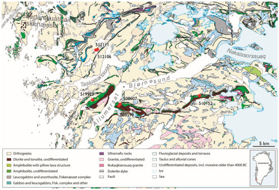
Figure 1.
Geological map of southern West-Greenland near the village Fiskenæsset. The localities of the samples used in this study are indicated with red dots. Map modified from GEUS [40].
At least three deformation phases affected the rocks in the area, where deformation was accommodated mainly by folding, but also by thrusting at a meter- to kilometer-scale. The region consists of several blocks or terrane that assembled into a larger unit at the latest part of the Meso-Archean age. The first regionally recognized deformation phase in the rocks can be observed in finely foliated isoclinally folded units (mica-schists, amphibolites, leucogabbroic rocks of the Fiskenæsset complex). The main deformation event metamorphosed the rocks in the area at amphibolite facies and granulite facies conditions. The effects of this main folding phase were overprinted by a later folding and thrusting phase at amphibolite facies conditions, before minor retrogressive overprint at greenschist facies conditions localized around late fault and shear zones. Uplift and erosion brought the rocks to the Earth’s surface [30,31,32,34,36]. The tectonometamorphic processes affecting the region developed a range of metamorphic features that are used as examples to highlight the visualization and quantification of metamorphic textures by AQM applying the Mineralogic software.
2. Materials and Methods
2.1. Sample Material
Six polished thin sections from metamorphic rocks from southern West-Greenland were coated with Carbon and investigated with SEM (ZEISS SIGMA 300VP; Cambridge, UK), see below. In the light of this study, no cross-checks were performed on the optical microscope. More details about the geological history of the samples were published previously [37,41]. Table 1 presents the analytical details for the investigated samples and Supplementary 1 gives sample and outcrop images as well as rock and mineral compositions as analysed with Mineralogic.

Table 1.
Analytical conditions for Mineral mapping. Mapping step size: three samples were mapped several times at different step sizes, see Section 3 (Examples of Applications) for details.
Samples 508599 and 508607 represent a finely layered volcanoclastic sediment collected from the Bjørnesund Supracrustal Belt (BSB). Hand specimen of sample 508599 is near-black with a slatey cleavage. It consists of quartz, andesine (plagioclase), biotite, amphibole, apatite, and pyrite. The rocks in the BSB were isoclinally folded at amphibolite facies conditions. The sample was collected close to an isoclinal fold core, and biotite in the sample clearly defines the shape of the fold and the foliation. Sample 508607 was collected from the same volcanoclastic unit in the RSB. However, in this sample contains quartz, anorthite, pale amphibole (anthophyllite based on field observations), biotite, and large garnets with inclusions of quartz, apatite, ilmenite, and rutile were grown over the main foliation.
Samples 521106 and 521111 show the reaction products between an ultramafic rock in contact with anorthosite or leucogabbro and intruded by a tonalite sheet. The anorthosite, leucogabbro and ultramafic rocks are part of the Fiskenæsset complex. The intruding tonalitic sheet causes a desilification reaction resulting in the formation of amphibole (anthophyllite, cummingtonite, gedrite or pargasite), phlogopite, and one or more aluminium-rich phases (cordierite, spinel, sapphirine and corundum (ruby)). Reaction temperatures are estimated to ca. 600 °C, using iso-chemical P–T-sections [36], with a gradient from lower granulite facies conditions in the western part of the Fiskenæsset complex to upper amphibolite facies close to the Inland ice sheet and in the southern part of the complex. The reaction occurred during the main folding phase in the region. Sample 521106 and 521111 are collected from Aappaluttoq, south of the village of Fiskenæsset, and here ruby is the main aluminium-rich phase resulting from the reaction. The sample consists of pale amphibole (gedrite), biotite, corundum, sapphirine, spinel, cordierite, anorthosite, hornblende, epidote, magnesite. Note that the peak mineral assemblage (gedrite, hornblende, ± biotite, cordierite, sapphirine; ca. 630 °C; 7 kbar [38]) does not contain quartz.
Sample 510152 represents a leucogabbro from the Fiskenæsset complex (Figure 1). The sample was collected in the southern part of the complex, where the complex lies in contact with the BSB. It consists of the minerals anorthite, Mg-rich hornblende, chromite and minor rutile. The amphibole in the sample is a result of deformation and metamorphism at amphibolite facies conditions, where it replaces pyroxene.
Sample 519923 is an amphibolite collected from the BSB. The hand specimen is dark green and finely foliated with a slatey cleavage. The minerals in the sample are distributed homogeneously, apart from tiny small faults filled with gouge and secondary minerals. Reactivated shear zones in the area accumulated gold in slightly enhanced concentrations. The sample contains anorthite, hornblende and the minor phases quartz, zoisite, rutile, sphene, apatite and zircon.
2.2. Whole Rock Geochemistry
Whole-rock geochemistry was carried out on a sample to characterize the bulk composition of these rocks. The analyses were carried out by Activation Laboratories (Actlab), Ancaster, ON, Canada, using their Research Lithium Metaborate/Tetraborate Fusion—ICP/MS analytical package. Samples 519923 was investigated, see Table 2. Both samples are described in more detail above.
Table 2.
Bulk geochemistry of each analysed thin section. For sample 511923, this data is compared to a whole rock geochemistry analysed by Actlab. Other data generated with Mineralogic (EDX analyses) in element wt% and recalculated to wt% oxides (and ppm for sample 511923). LOI: loss on ignition. Numbers in italics are estimates only.
2.3. Mineralogic Method
The micro-analysis on the selected thin section was performed on a ZEISS SIGMA 300VP SEM equipped with a back-scattered electrons (BSE) detector and two Bruker XFlash 6ǀ30 EDX detectors, with 129 eV energy resolution and with the ZEISS Mineralogic automated quantitative mineralogy software platform located at the Geological Survey of Denmark and Greenland, Copenhagen, Denmark. The description of the Mineralogic method in this section, including screenshots (Figures S1–S7) from the set-up of the Mineralogic recipes can be found in the Supplementary 2. Within each thin section, a region of interest was selected and imaged to provide a high-resolution BSE mosaic of stitched images. Also, on this region of interest, a quantitative mineralogical analysis was carried out using Mineralogic, creating a mineral map with a user defined step size (or pixel size) as well as a list with parameters for grains in the sample. The acceleration voltage of the primary electron beam was set to 15 or 20 kV, to ensure X-ray excitation for all relevant elements (e.g., Fe, Cu, Zn). The 120 µm aperture providing 80 µA beam current used was used to obtain a high input count rate for the EDX detectors. The EDX software is fully integrated with the Mineralogic software, allowing for matrix corrections of each mineral. Therefore, the exact element concentrations can be calculated for each acceleration voltage. A detailed description of the Mineralogic method is given below:
2.3.1. Zeiss Mineralogic Mining
The ZEISS Mineralogic software platform has a Mining and a Reservoir rock plug-in, though analytical functionalities between both branches largely overlap. The difference between both lies in how obtained data are visualized, e.g., as target and byproduct (Mining), or integrated with porosity measurements (Reservoir). Here, the Mining part of the software was applied. The software offers a recipe-based solution for all steps in the analysis (SEM parameters, holders and stubs used, calibration for the EDX and BSE detectors, image analysis, morphological analysis, mineralogical analysis, lithological analysis, mining output parameters, and criteria that specify how and when the analytical run is performed and terminated). These recipes can be saved, mixed, and changed individually, thus adapting each analysis to the sample at hand. Recipes can also be in- and exported allowing for an exchange between different internal and external users. Routine analyses can be set up allowing a non-geologist/mineralogist can run samples from a batch of similar samples, while the more experienced user gets the freedom to vary many parameters for each analysis [8]. The description here is based on Mineralogic software version 1.6.
2.3.2. Image Navigation
The Image Navigation tool of the ZEISS SEM applies digital images of thin sections, the entire sample holder, or overview SEM-images to navigate within the sample (Figure S1). The tool allows the user to define three fiducial points on the navigation image and connect those to stage coordinates, afterwards the movements of the stage can be controlled from the navigation image. The tool is especially ideal to set up analyses on holders with several samples, or on fine grained material in a fast manner.
2.3.3. SEM Recipe
In this recipe, the SEM can be operated in a normal mode to set and save the operating conditions for the analysis. The sample can be placed to the correct position, the beam is focused and optimized at the required acceleration voltage (often 15–25 kV) and aperture size (often 60–120 µm). The brightness and contrast of the image are set. The SEM recipe saves the current settings of the SEM (like vacuum settings, beam parameters) and regulates the SEM imaging parameters (dwell time to allow for stage movements, scan speed), see Figure S1.
2.3.4. Holder Recipe
In the Holder recipe the size and shape of both the sample holder and of the individual stubs can be defined and adjusted. First the size and shape of holder are defined (holder set-up), afterward the size and shapes of the individual stubs (stub setup). The recipe lists a number of standard sample holders, but own holders can be defined as well (Figure S2). In the stub details part of the menu, the geometrical parameters for the analysis of each particle can be defined: Z-coordinate of the stage, magnification during the analysis, step size for the mapping of the sample, and the area or areas in the sample that are analysed (Figure S2).
2.3.5. Calibration Recipe
Both the BSE brightness and the EDS peak position can be monitored and corrected during larger mapping sessions. The BSE brightness is regulated using a standard with a bright- and a dark phase next to each other, e.g., a copper–aluminium stub. The brightness of the BSE image is set such that the bright phase in the standard (e.g., copper) has grey-values in the upper grey-level segment, but is not completely white, while the dark phase (e.g., aluminium) has grey values in the dark-grey segment. The interval for monitoring can be selected, e.g., every hour and for every new sample. At each monitoring event, the SEM resets the brightness and contrast values of the SEM to match the predefined values for the bright and dark phase in the standard (Figure S3).
The EDS peak position can be monitored by regularly measuring suitable EDS peak, typically Cu Kα, for the beam energy settings chosen for the analysis.
2.3.6. Image Processing Recipe
Mineralogic analyses are typically performed overlying a BSE image, but other types of images based on electron microscope detector input, like secondary electrons or cathodoluminescence (CL) signal can be applied too, where required. The image can be thresholded to only include certain grey levels for the forthcoming Mineralogic analysis, e.g., with the aim only to investigate the brightest phases in the sample, or to exclude epoxy and porosity from the analysis. The quality of the image can be improved with a large number of image processing techniques like arithmetic functions (e.g., addition, substraction, inversion), logical operations (e.g., image AND image, image OR constant), convolution and filters (e.g., median filter, sharpening, edge detection), histogram and threshold operations, morphological operations (e.g., dilation, opening, hole fill, skeletonize), segmentation and region based operations (e.g., watershed) or geometric and linear transformations (e.g., downsize with a power of two).
The image processing recipe tap can also be applied on pre-set functions like the search for bright phases in the sample (Figure S4), which can be applied to find suitable zircon or monazite minerals for isotope dating or certain ore minerals). Here, the BSE signal is thresholded to only find the brightest particles in a large sample and to store their chemistry and coordinates.
2.3.7. Morphology Recipe
In the Morphology recipe the grain size, grain shape and other physical parameters of the sample that are analysed can be selected. The software offers following possibilities: area, length, breadth, elongation, roughness, Feret maximum, minimum, and mean length, Feret maximum, minimum, and mean angle, porosity, and grey value (Figure S5). These grain morphology parameters are provided as output data for every individual analysed grain and can therefore be correlated to grain mineralogy or chemistry. Morphological analyses are performed on the BSE (or other input) image of the sample, not on the map produced during the analysis.
The morphological parameters can be classified such that grains full-filling certain size or shape parameters are registered separately. The grains fulfilling these parameters can be filtered out after the analysis.
2.3.8. Mineral Recipe
The Mineral recipe is the central part of the Mineralogic Mining plugin. It regulates the EDS and mapping type parameters, holds the list of minerals, and allows for morphochemical classification criteria (Figure S6). The Mineralogic analysis can be performed in five different ways:
- Mapping analysis, where the user defines the step size (pixel size) for the EDS map, and an analysis is performed for every single point (pixel) of the map. Typical pixel sizes are 5–30 µm, but can be larger for coarse grained, homogeneous samples, or as small as 200 nm [20]. This method presents the full detail of the sample but is also the most time-consuming method.
- Spot centroid analysis, where the sample is segmented by BSE value of the grains. The method is typically used on grains in an epoxy matrix. For each grain determined, the geometrical centre of the grain is calculated, and a single EDS analysis on this point is performed. This method is especially suitable for homogeneous grains, as a small variation in the chemistry, like inclusions or zonations, will not be picked up.
- Feature scan analysis, where—like for the spot centroid analysis—the grain boundaries are determined by segmenting the BSE image. In this analysis mode, the beam is rastering within the boundaries of the grain, giving an average chemical composition. In case of zonations, a more correct average grain chemistry will be found; for heavily included samples, a false mineral classification might be generated. The method can be nearly as fast as a spot centroid analysis, depending on the pre-set amount of counts in the spectrum.
- Fast scan is an intermediate form of Feature scan and spot centroid analysis. It scatters a series of point analyses across a grain and thus arrives at an average composition of the grain. The user gets to determine the density of the spots for the analyses in an area, but each grain is analysed at least once, independent of its size.
- Line scan analysis, where all EDS analyses are made along a line with a pre-defined step-size across the centre of a particle or frame. All variations in composition are accounted for, and a first impression on the grain size and texture can be obtained. The method is very fast compared to a full Mapping analysis.
- Grey level mapping, where the sample is imaged (usually with BSE), without applying EDS measurements. For samples with a simple chemistry, grey values can be used to separate individual minerals. The method is very fast, but less precise than EDS-based investigations.
For all EDS-based methods, the EDS spectrum deconvolution can be specified in the same way as for regular EDS analyses (Figure S6a). Thus, elements can be excluded from quantification (e.g., carbon used for coating is set to deconvolution-only), matrix quantification methods can be chosen (ZAF vs. Phi-Rho-Z), spectra output data can be normalized, and elements can be chosen to be always or never included, if wished for, thus potential sources of peak overlap can be avoided. EDS dwell time, and detector throughput rate can be chosen by the user. Every single generated spectrum during the analysis is fully quantified and the weight percentages of each element in each pixel on the false coloured mineral map is available after the analysis. User can choose to add standards-based quantification of the spectra. These latter two points are unique for the Mineralogic software. The matrix quantification for each spectrum also allows the user to switch between different acceleration voltages in between samples, without the need to specify a new mineral list. Most AQM systems require the user to make separate mineral lists for each acceleration voltage.
The mineral list for the sample analysis is created by the user based on the element wt% of the mappable phases and can be used to produce a variety of visualizable informative image and data outputs. For each mineral the range of tolerated concentrations for each element, as well as for ratios between two elements, can be used to define the mineral phase (Figure S6b). Minerals are placed in a list, which is checked against the chemistry of each analysed point, following a first-match principle and based on the order of minerals in the mineral list, which is defined by the operator. The same principle to build mineral lists can also be used to define element concentration maps or element ratio maps, where individual phases are identified and coloured by the concentration of one or a few elements. Mineral lists can be exported and imported between projects and adjusted to fit the exact mineral specifics for the sample area of interest, allowing for slight differences in mineral chemistry resulting from different whole rock compositions or metamorphic temperatures.
In an addition tab in the recipe, minerals can be clustered into groups (e.g., albite, labradorite and anorthite as plagioclase). Clustered minerals can be integrated as a group when particle data is exported after the analysis.
Additionally, morphological criteria can be used in the classification of minerals. For example, textural properties can be defined based on the chemically mapped grains, where the grain size or shape properties are used to synergize the chemical and textural characteristics. For example, zircons of a size large enough to be dated with a laser connect to a mass spectrometer can be classified from the main zircon population separately. All different ways of describing the sample (e.g., element map, mineral map, morphochemical map) can be calculated offline from the generated data. There is no need to reanalyze the sample after the mineral list was changed.
Many parameters affect the speed and quality of an AQM analysis, and a Mineralogic analysis is no different. Each analysis must be optimized prior to an AQM run. Different types of analyses (see above) will yield a difference in analysis speed and data quality. Acceleration voltage and aperture size both control how much signal reaches the EDX detectors, where a high acceleration voltage and a large aperture size result in a greater signal. These parameters are typically tailored to the nature of the question (i.e., the data required), according to which the resolution and speed can be adapted. Detector throughput rate can be adjusted to optimize the measurement accuracy and precision. The throughput amount (i.e., counts input) impacts the elemental energy peaks full width half maximum (FWHM) and therefore the accuracy and precision. The dwell time (time the beam stays at one spot before moving on) has a major impact on the analysis speed. The lower a dwell time the faster the analysis is, however if the dwell time is too low it will result in insufficient spectrum counts for a good quality analysis. Image capture time, determining the quality of the BSE image, and frame magnification, determining the amount of stage movements, also affect the analysis time, but these effects are minor and have no real influence during a mapping analysis. The last parameter to affect the analysis speed, is the step size (pixel size) in the mineral map, where a smaller step size will increase the analysis time, but at the same time will provide a more detailed in-depth analysis.
2.3.9. Mining Recipe
In this part of the software, particular minerals of interest and elements can be selected to perform advanced textural and chemical quantification. In the “Assay” part of the user interface, the user has the ability to select the elements of interest in this sample (Figure S7). The software will then perform an assay measurement, whereby the chemically quantified pixel data and the specific gravity (data that is added to each mineral classification) are used to calculate a mass. This is done for all pixel/elements selected across the sample and is used to calculate an assay. This can therefore be used as a rough “bulk rock assay” where the analysis is based on a single 2D plane throughout the entire sample.
Additional value can be gathered from this aspect of the software whereby “elemental distribution” data can be gathered. This is where the chemical distribution is quantified. For example, when the chemical distribution of Mn is of interest: the data will give the wt% amount of Mn in all specified minerals, and also a distribution percentage based the total percentage of Mn found in each phase. This data is provided from the directly chemical quantification during the automated analysis and not from idealized or pre-defined concentrations. This provides researchers with a more reliable AQM technique to understand and quantify chemical and mineralogical variations. However, in cases where element concentrations cannot be measured reliably (e.g., for Boron in tourmaline), a concentration can be assigned in the mineral list for that specific element.
The minerals to be analysed for the map can be selected, as Target minerals. Byproducts and Gangue minerals can also be defined. The example shows a sample with a mineral list with a morphochemical classification (Figure S7). The mutual interconnection between minerals can be described by defining the liberation parameters, which can be exported for all minerals after analysis, together with the association and interlocking data.
3. Examples of Applications
3.1. Mapping Speed and Composition
Sample 511923 was analyzed with the purpose of investigating how different types of Mineralogic analyses (line scan and mapping) and a variation in step size affect the analysis speed and results in a fairly homogenous sample. In total six different analyses at 235.2× magnification were run on the same 0.5 × 0.5 cm area of the sample (Figure 2) consisting of 20 frames. Two line-scan analyses with 10 and 20 µm step size, plus four mapping analyses with step sizes ranging from 40 to 5 µm were carried out on the same area of the sample. The parameters for the analyses were the same using 20 kV acceleration voltage, 120 µm aperture, 275 kcps throughput rate for the EDX detector, and 0.004 sec dwell time.
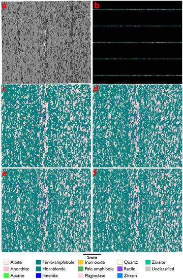
Figure 2.
Same area of sample 511923 analyzed with different methods. (a) BSE image. (b) 20 µm step size line-scan. (c) 40 µm step size mapping. (d) 20 µm step size mapping. (e) 10 µm step size mapping. (f) 5 µm step size mapping. For analysis times see Table 3. The 10 µm step size map consists of 244606 analysed pixels.
The line-scan analyses both completed in just around 4 min, and the most time consuming of this type of analysis is to capture the (BSE) image prior to analysis. For the mapping analyses, there is a huge increase in analysis time, when decreasing the step size (see Table 3).
Table 3.
Comparison between most abundant and selected other minerals between the different analysis methods in area % for different step sizes in line scanning and mapping. STD = standard deviation. Sample 511923: 24 frames at 235.2× magnification (ca. 0.5 × 0.5 cm). Sample 521106: 220 frames at 235.2× magnification (1.5 × 2 cm).
As seen in Figure 3, the distribution of mineral phases between the runs are very similar. Also, when looking on the standard deviation for each mineral phase between the different analysis, there are only small differences (Table 3). However, there are more minor phases picked up by the 5 µm mapping method than the other methods. With the line-scan methods no zircon or rutile were analyzed, however both phases were present in all of the mapping methods. Line scan does not find all minor phases in the sample, and in foliated samples detected small equidimensional phases may get overrepresented when scanning perpendicular to the foliation.
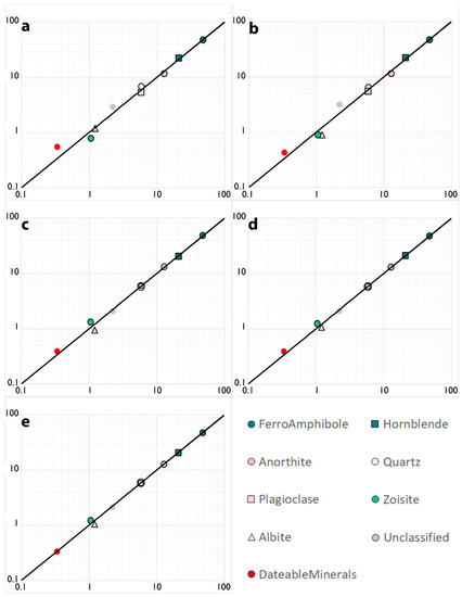
Figure 3.
Logarithmic diagrams comparing the different analysis methods (y-axis) against the most time consuming and most detailed 5 µm step size mapping method (x-axis). Data is shown as area %. (a) 20 µm step size line-scan. (b) 10 µm step size line-scan. (c) 40 µm step size mapping. (d) 20 µm step size mapping. (e) 10 µm step size mapping. Dateable minerals are zircon, apatite, rutile and sphene.
We use the more inhomogeneous sample 521106 to investigate how the different analysis methods apply on a more complex sample. The setup is similar to that used for sample 519923, except for the area analyzed, which is 220 frames at 235.2× magnification (1.5 × 2 cm) (Figure 4), and only one line-scan, at 20 µm, was applied (Figure 5). The results are similar as well, with zircon not identified in the line-scan analysis. Otherwise, the different step sizes in the mapping analysis produce results with minimal variations (Figure 5; Table 3).
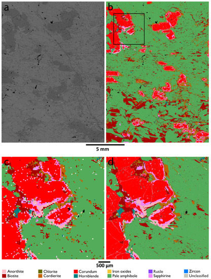
Figure 4.
BSE and Mineral maps of sample 521106 and a selected area for comparing the map quality between different step sizes. (a) BSE image consisting of 220 frames. (b) 5 µm step size mineral map (ca. 9 million pixels). The square indicates the position of details in (c,d). (c) Selected area mapped with 40 µm step size. (d) Selected area mapped with 5 µm step size.
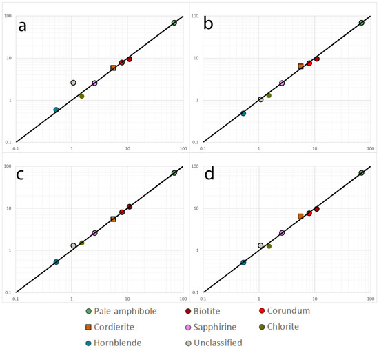
Figure 5.
Logarithmic diagrams showing the correlation between different analysis methods (y-axis) and 5 µm step size mapping (x-axis). Data is shown as area %. (a) 20 µm step size line-scan. (b) 40 µm step size mapping. (c) 20 µm step size mapping. (d) 10 µm step size mapping.
The line-scan feature has proven to be very useful as a way of obtaining a quick and precise overview of the geochemistry and major element mineralogy of the sample. Also, a more detailed mineral list can be built from the line scan runs. Where the focus of investigation lies on the chemistry and mineralogy, line scan is a good alternative to running a full map. However, many textural features (e.g., zonations, reaction rims, included minerals) and accessory minerals are not picked up by line-scan analysis.
Mineral mapping at a large step size (here 40 µm in 8 min for 20 frames and 83 min for 220 frames) also is a very fast analysis and gives a good overview of the entire sample (see Figure 2 and Figure 4 to compare image quality). Afterwards ares can be chosen for a more detailed analysis with the mapping feature at a small step size. This two-step procedure is faster than mapping the entire sample at a small step-size. The difference in step sizes generally has little influence on the mineralochemical data (Figure 3 and Figure 5), however details like zonations or reaction rims are often not detected with a larger step size (Figure 4).
3.2. Garnet with Quartz Inclusions
In sample 508607 large garnet grains were observed, which were investigated for their chemistry and mineralogy in order to gain more information on the metamorphic history of the volcanoclastic rocks. The sample was collected from the same unit of volcanoclastic sediments as sample 508599 discussed below. However due to lithological variation, its bulk composition is different (less Na, less K, less Si, more Ca, more Fe, more Al, see Table 2), which is expressed in a different mineralogy: quartz, anorthite, biotite, pale amphibole, garnet, apatite and pyrite. In the most biotite-rich amphibole-poor layers, large garnets have grown with the foliation bending around them (Figure 6). In the garnets, inclusions of apatite, rutile, ilmenite and especially quartz are present. The quartz is irregularly shaped with lobes intruding into the garnet. All inclusions are only found in the center of the garnets, but not in the rim. Pyrite is partially oxidized and is found in association with biotite.
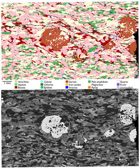
Figure 6.
Mineral map (a) and BSE micrograph (b) for the volcanoclastic sediment with garnet porphyroblasts. The mineral map contains 281714 pixels.
The sample was imaged with the BSE and CL detectors, as well as analyzed for its mineralogy and chemistry, all with the Mineralogic software. In the SEM recipe of the Mineralogic software, the detector for imaging can be selected and changed to CL in order to make a stitchable series of images automatically. After creating a Mineral map (Figure 6), the Mineral recipe was applied to generate element concentration maps for the main elements in garnet (in Figure 7 Mg, Fe, and Ca are shown). The element concentrations displayed are true wt% concentrations, not relative intensities. Furthermore, the quality of the EDS systems was monitored with point analyses on silicate standards and yields an error < 1 wt% compared to electron microprobe analyses, with slightly too low values for light elements and too high on the heavier elements (see Supplementary Table S1).
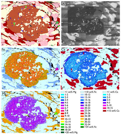
Figure 7.
Detailed maps and image of the central garnet in Figure 6. (a) Mineral map. See Figure 6 for a legend of the colours applied. (b) Cathodoluminescence image mosaic of the same garnet. White and black arrows point to growth features in anorthite and quartz, respectively. (c) Mg element concentration map. (d) Ca element concentration map with black contours indicating the weak zonation in garnet. (e) Fe element concentration map. Arrows in (c,e) point to an example of an included biotite grain with different Mg–Fe ratios.
The mineral map (Figure 6 and Figure 7a) reveal that the inclusions in garnet are mainly observed in the core and inner rim of the garnet. The core of the garnet mainly yields quartz and biotite (plus pyrite) inclusions, while ilmenite, rutile, amphibole and apatite mainly, but not exclusively, are observed in the inner rim. The inner rim does not show biotite inclusions.
CL investigations show that the quartz inclusions in the garnet consist of smaller grains healed into larger inclusions (black arrows in Figure 7b). Anorthite adjacent to garnet reveals growth rims in CL (white arrows in Figure 7b), which are most strongly on the left and right sights of the grains.
EDS analyses of the garnet showed ca. 19% Si, 13% Al, 2% Ca, 5% Mg and ca. 26% Fe. There is some Mn present as well (~0.5 wt%), but no Cr (less than 0.5 wt%, usually not detectable). There is a minor compositional variation between the core and the two rims of the garnet, with no difference in Si and Al (less than 1 wt%), but slightly lower Ca and higher Mg and Fe in the inner rim and slightly higher Ca, lower Mg in the outer rim (the difference in concentrations between the core and rims is always less than 2 wt%). These zonations are just visible in Figure 7c–e. With image manipulation (inversion of Ca-image, followed by adding the images together in Adobe Photoshop©), these differences can be enhanced and mapped. Figure 7d shows the contours for the weak zonation, based on Fe, Mg and Ca concentrations. The small variations in the chemical composition are visible in the garnet ternary diagram (Figure 8), where the XMg–XFeMn–XCa composition of the garnets in Figure 6 are plotted based on pixel-by-pixel data exported from Mineralogic analyses of the garnet. The garnet is an almandine, which are typical for aluminous rocks deformed at amphibolite facies conditions.
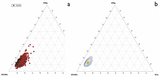
Figure 8.
Ternary diagram showing the garnet porphyroblast minor element composition expressed as XMg–XFeMn–XCa. (a) Data for 6400 representative pixels; (b) Contours showing the data intensity of (a). The Figures are plotted applying WxTernary [42].
The garnet in this samples has probably grown from a quartz consuming reaction, possibly chlorite + quartz + muscovite = garnet + biotite + H2O, which can explain for the biotite and quartz inclusions in the core of the garnet (Figure 6 and Figure 7). From the element concentration plots (Figure 7c,e) can be seen that the composition of the biotite in the inclusions is different from the biotite in the foliation: the included biotite is Mg-rich, while the biotite in the foliation is Fe-rich. The inner rim of the garnet showed a continuation of the same reaction, probably at a slightly higher temperature, thus slightly changing the Fe–Mg concentration in biotite and garnet [43] (Figure 7). Ti is largely incompatible in aluminous garnet and remains as ilmenite and rutile inclusions. The foliation of the rock bends around the previously formed garnet and some biotite is formed in the pressure shadows demonstrating a weak dextral sense of shear (Figure 6 and Figure 7). The fractured and healed quartz and anorthite visible in the CL image show that deformation might have been fast and intense, as quartz and anorthite typically are deforming plastically at garnet-forming temperatures [44,45]. Large rims around anorthite show that anorthite precipitated under a differential stress from fluids during metamorphism (darker rims of anorthite visible in the CL image (Figure 7b) are thicker along the horizontal grain axis than the vertical). Ca in garnet may also originate from these fluids.
3.3. Reaction Rims Around Rubies
The ruby-bearing sample 521111 from the Fiskenæsset complex contains the reaction products of the interaction of a tonalitic sheet intruding into an ultramafic rock in contact with anorthosite. As not all of the ruby in the thin section is of gem-quality, we refer to the ruby as corundum. The reaction occurred at amphibolite-facies metamorphic conditions, i.e., post peak-metamorphism (which was at granulite facies conditions) [37,41]. It has been discussed previously whether the alumina of corundum and other aluminous minerals (spinel, kornerupine, cordierite, and sapphirine) are primary or secondary minerals [37,38,41,46]. Reaction temperatures are estimated to be ca. 600 °C, for the southern part of the complex [37,41], but may have been higher nearer to the village of Fiskenæsset where the current sample was collected. with a gradient from lower granulite facies conditions in the western part of the Fiskenæsset complex. The corundum-forming reaction occurred during the main folding phase in the region [37].
Like for the garnet example above, the sample was mapped for its mineralogy, and afterwards recalculated with new mineral lists to create mineral association maps and an element ratio map (Figure 9 and Figure 10). The mineral association maps can be made in the Mineral recipe tab by redefining the colours of the minerals, highlighting two or three phases, while all other mineral phases are displayed in white. As for the element concentration maps, the mineral list can also be redefined to show steps in element ratios in order to display e.g., changes in Si/Al or Fe/Mg ratios in the sample.
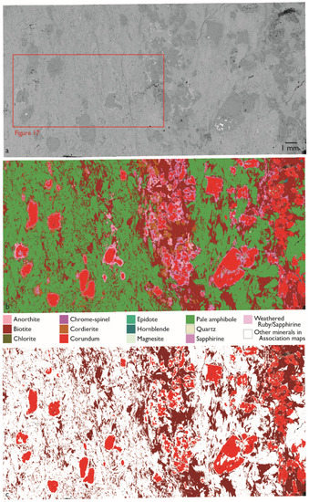
Figure 9.
Corundum (Ruby-)bearing rock showing the mineral assembly after the formation of corundum, sapphirine, cordierite, anorthite, pale amphibole and biotite (peak metamorphic reaction products) and the retrograde reaction products magnesite, chlorite, and quartz. (a) BSE image of a selected part of the sample. (b) Mineral map of nearly the entire thin section of the sample (1.63 million pixels). (c) Mineral association map of biotite and ruby. All other minerals are displayed in white.
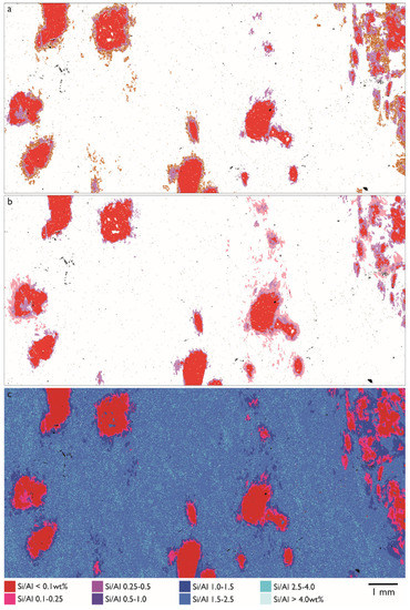
Figure 10.
Detail of the sample displayed in Figure 9. (a) Corundum-sapphire-cordierite association map. (b) Corundum-sapphirine-anorthite association map. All other minerals are displayed in white. (c) Element ratio map showing the Si/Al ratios in the sample. wt% indicates that wt% data were used to calculate the ratios. Legend for (a,b) in Figure 9.
Desilification of the ultramafic rock results in the formation of pale amphibole (mainly gedrite), biotite, and one or more aluminous phases (cordierite, sapphirine and corundum), e.g., by the reactions: olivine + K-feldspar (tonalite) + H2O = biotite + anthophyllite or olivine + SiO2(aqueous) (tonalite) = anthophyllite [41] (Figure 9). The intruding tonalite is not peraluminous and can therefore not be the source of aluminium, however anorthite is able to react in a balanced reaction: olivine + anorthite + H2O (tonalite) = Ca-bearing amphibole + corundum [41]. In the case of sample 521111, where reaction temperatures may have been slightly higher, the corundum mineral is surrounded by two rims of reaction products (Figure 9b and Figure 10a,b). Corundum in the centre, sapphirine around the corundum, and cordierite or anorthite around the sapphirine. The reaction rims are very well developed with the same width all around the corundum minerals, no symplectites or other fine-grained minerals are observed in the reaction rims, which are therefore interpreted to have developed near-simultaneously with the corundum-forming reaction at peak or near-peak metamorphic conditions. Figure 10c indicates that the minerals formed in the reaction rims are increasingly rich in Si compared to Al, ranging from no Si in ruby to more Si than Al in cordierite. This shows that the degree of silica-desaturation of the rock may have fluctuated during the ruby-forming reaction, or that the Al from the original anorthite was consumed towards the end of the reaction series. Cordierite or anorthite as the outer reaction rim, occur systematic (Figure 9b and Figure 10a,b) and may reflect the original hornblenditic and anorthitic layers, respectively, in the anorthosite before intrusion of the tonalite. Biotite is not associated with corundum (Figure 9c), but cordierite seems more strongly associated with biotite, than anorthite (Figure 9b). Here, sapphirine and cordierite are peak metamorphic minerals, ruby started growing just before peak metamorphic conditions, sapphirine and ruby are part of the peak metamorphic assemblage, and cordierite and anorthite grow immediately after initial decompression [42], as was also observed in other parts of the Fiskenæsset complex [37,41]. However, a decrease in temperature could additionally create retrograde sapphirine or plagioclase, as also was described previously for other parts of the Fiskenæsset complex [46].
3.4. Grain Size Distribution of Chromite in Leucogabro
Within the Fiskenæsset gabbro and leucogabbro thin layers of chromitite have been observed, which previously have been investigated for their platinum group elements content [34,47]. Within the Fiskenæsset complex both primary and secondary chromite occur [48]. The chromite in the layer is homogeneous in composition but shows a wide variation in grain size. The chromite grains are situated in the Mg-rich hornblende layers of the metamorphosed gabbro (Figure 11a), while only a few grains are associated with anorthite. The chromitite is highly dominated by chromite (Figure 11b), thus individual chromite grains are touching each other, which makes automated grain size analysis more complex.
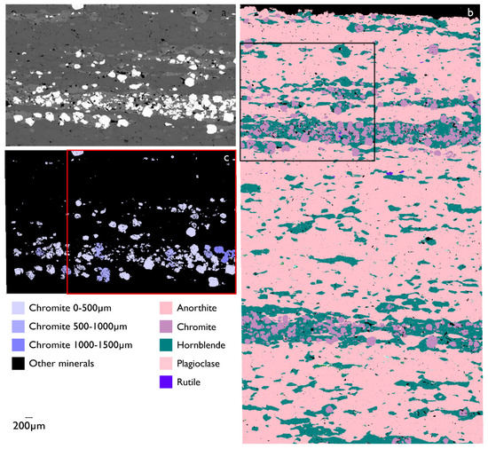
Figure 11.
Leucogabbro with bands of chromite, sample 510152. (a) BSE micrograph of part of sample, showing chromite grains in white. (b) Mineral map of a larger part of the same sample. Chromite is associated with hornblende. 1.63 million pixels. (c) Grain size map showing the same part of sample as in (a), with colour-coding of the chromite grain sizes. (a,c) partially overlap with the upper left part of (b), indicated with squares in (b,c).
In order to measure the grain sizes a modified version of the watershed method, which the image processing tap of the software provides, was applied. After thresholding to select the chromite grains from the rock, the image was eroded in three iterations, followed by dilation, as a modification of the opening function that is routinely applied—this gives better separation of individual grains. The watershedding was set to 40 units difference in order to separate touching grains. After image processing the chromite was selected by mineral classification (minerals tab) and characterized by morphology and chemistry in the same tab.
The association data for sample show that 54% of the chromite is in contact association with hornblende and only 17.1% with anorthite, while 23% is associated with the background (mainly holes and cracks between chromite grains) and the remaining fraction of the association is made up by minor phases including rutile and chrome-spinel. The grain size distribution of the grains is visualised in Figure 11. It shows that individual chromite grains in this layer range in size (Feret mean diameter) from 100 to 1000 micrometer. Part of these grains are clusters of several grains, despite the watershed procedure during the image processing. Chromite settled together with hornblende during the cumulation of the igneous rock. Individual chromite grains were already inter-grown during their crystallization and their grain size and texture have not been affected by metamorphism. The chromite grains in this sample are primary minerals. An analysis of the roundness and orientation of the individual grains (Feret angle) shows that the chromite grains are not systematically flattened during the three tectonometamorphic events that affected the area, showing that the chromite grains are very rigid under those tectonometamorphic conditions (ca. 600 °C, 5 kbar [37,41]).
3.5. Maximum Feret Angle Determination
Sample 508599 was investigated for the size and orientation of the biotite minerals in the thin section, which define the foliation and the isoclinal fold in the sample. The orientation of the biotite minerals can be described with the maximum Feret angle. The maximum Feret angle is the angle between the maximum Feret diameter of a particle and the horizontal axis. The maximum Feret diameter is the longest diameter of irregular shaped particles.
In order to measure these morphological features for biotite in the volcanoclastic sediment, in the image processing recipe the BSE image of the sample (Figure 12A) was thresholded by grey scale value to only investigate the minerals with a bright BSE contrast; these include mainly biotite and a few accessory phases. The biotite grains are now isolated features of single grains or clusters of grains that lie in a darker matrix. The biotite grains can thus be investigated with a spot centroid or feature scan analysis. The mineral list was adapted to show all none-biotite grains in black, while a morphochemical criterion was added to the biotite classification in order to classify the biotite grains in colours according to their Feret angle (Figure 12B). The results are shown in Figure 12, together with the BSE image and the mineral map of the entire thin section.
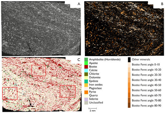
Figure 12.
Isoclinal fold in a volcanoclastic sediment containing biotite, amphibole, anorthite and quartz. (A) BSE micrograph of the sample. The three main phases (biotite, anorthite and quartz) are light, intermediate and dark grey respectively. (B) Maximum Feret angle map over the thin section. All none-biotite minerals are black, while biotite is coloured by its maximum Feret angle. Positive and negative angles are indicated in the same colours. (C) Mineral map showing the distribution of the mineral phases in the sample. This mineral map contains 2.04 million pixels. Squares define three smaller areas within the sample, with their own data for surface area and association data.
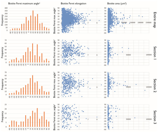
The BSE image and the Mineral map show a different behavior for the individual minerals in the sample across the isoclinal fold. In the flanks of the fold, biotite occurs in clusters of grains. Individual grains are occasionally oriented randomly, but the larger clusters of grains are oriented into elongated clusters with low Feret angles (preferentially 20–40°; see Figure 13), while most individual biotite grains and smaller clusters have lower Feret angles (mainly 0–20°) and are stacked stair-case-wise to follow the local foliation. Thus, the individual grains follow the main foliation in the area (oriented ca. 0–10° with respect to the horizontal axis), while they form stacked arrays that follow the local foliation (20–40°) in the individual fold flank. In the core of the fold, biotite occurs more scattered, and all Feret angle orientations with an large elongation are observed between −30 and 40° (Figure 12 and Figure 13), while the grains with the largest area have orientations around 40 and −10° (Figure 13), fitting with the orientation of the two flanks mapped in Area 2 (Figure 12). In the least deformed part of the fold (Area 3) biotite grains are smaller and show no preferred orientation for the most elongated grains (Figure 13).
In the less extensively deformed parts of the fold, quartz and plagioclase occupy roughly the same percentage of the area (compare least deformed Area 3 to intensively deformed Areas 1 and 2 in Table 4). Both minerals are partially intermixed but prefer to cluster with their own phase. In the flanks of the fold, a more well-defined layering of quartz, biotite and anorthite occurs, where both quartz and biotite are sandwiched between layers of anorthite. In the core of the fold, hardly any quartz minerals are observed. Biotite is associated with anorthite (Figure 12C and Figure 13). This is illustrated for association data for the three areas in Figure 12C (see Table 4). Area 1, derived from the core of the fault, and Area 2, derived from the flank, show that biotite is strongly associated with plagioclase (45.3 area% and 48.7 area%, respectively), while in the least deformed Area 3 this association is only 34.0 area%. Plagioclase in the flanks of fold (Area 2) is strongly associated with biotite (45.3 area%), and the association with quartz is the least of the three areas (34.5 area%). Plagioclase in the core of the fold (Area 1) is forming the sandwiching layer between biotite (37.8 area% association) and quartz (40.9 area%). In the least deformed part of the sample, plagioclase is strongly associated with quartz (51.6 area%) and much less with biotite (21.3 area%), which is partially caused by a much lower area% of biotite in this section.
Table 4.
Area% and association data for biotite, quartz and plagioclase in the three areas indicated in Figure 12C. TS = thin section.
Folding in the area occurred at ca. 600 °C [37,41]. Under these conditions all three minerals (quartz, anorthite and biotite) deform plastically under most strain rates [44,45]. Quartz, which under these conditions is more plastic than plagioclase, moves to the flanks of the fold, while the more rigid plagioclase is pressed towards the cores of the fold (compare Areas 1 and 2 in Figure 12C and Table 4). Biotite rotates by a combination of recrystallization and mechanical fracturing and healing to accommodate to the main stress in the region and can be used to read the record of the main foliation outside the isoclinal fold (Figure 13), i.e., 0°. However, the movement of quartz and plagioclase also force the biotite to follow the local foliation, leading to a stacking of horizontally oriented minerals into a local foliation of ca. 30° to the horizontal fold axial plane (compare to Figure 13). Continued stress on the rock will remove the evidence for a fold core from the record of the rock, leaving the sample layered by mineral phase and with clusters of flat-lying biotite. We are thus able to study the generation of a schistose layering from an initially little deformed rock in a single sample by studying individual areas of the fold core.
4. Discussion
The five examples of application above show a small set of the vast range of possibilities for modern AQM systems, like Mineralogic, where visualization of the data and the generation of chemical, mineralogical and morphological data are combined. Traditionally, mineral compositions in metamorphic rocks are quantified with optical microscopy or microprobe analyses, while metamorphic textures are investigated with optical microscopy and often unquantified or, mainly in case of deformed samples, quantified by electron back-scatted diffraction. By applying AQM, visualization and quantification can be combined in one tool and executed on the same minerals. The AQM software is creating a false-coloured mineral map, while simultaneously measuring grain morphology and chemistry. The false-coloured map resembles the optical microscope mineral display of metamorphic textures, but also forms the basis to gain quantitative data for the sample. Compared to the microprobe, AQM offers mineral maps and not only element maps. This is combined with the higher analytical speed for EDX analyses compared to the wavelength dispersive spectrometry analyses on the microprobe. The diversity and flexibility in the chemical, textural and mineralogic visualization is demonstrated in this paper as a means of contextualization of what can initially be complex data sets.
AQM is often regarded as a slow analytical tool. However, depending on the information required, analytical speed can be adapted to the optimal combination of mineralochemical precision, map-quality and time. An area of 1.5 × 2 cm can be analysed in 83 min at a 40 µm step size, and provide almost identical mineral concentrations, when compared to runs with smaller step sizes and longer analysis times (Table 3; Figure 3 and Figure 5). A time-saving approach could be to first run a large (here 20 µm) step size line-scan or Mineral map (here 40 µm step size) on the selected sample, then build a solid mineral list and run selected area(s) with a smaller step size to obtain detailed information on specific features e.g., reaction rims. Further, these investigations indirectly showed that the general reproducibility of the data, even while generated at different step-sizes (pixel sizes), is good.
Within the Mineralogic software platform, it is also possible to analyze samples with different acceleration voltages, without changing the mineral list. Samples 521106 and 521111 originate from the same area, were analyzed at 20 and 15 kV respectively, and were recalculated with the same mineral list without any adaptions (Table 1).
The garnet and ruby examples outline unique capabilities the Mineralogic software is able to access when compared to other AQM platforms. Because Mineralogic’s EDX software is matrix-correcting and quantifying every spectrum for every pixel in the mineral maps and for each spot or feature scan for every epoxy-embedded particle, the exact chemistry is known with the same precision as for EDX point analyses. Elements can be easily detected with concentrations down to ca. 0.5 wt%, and major and minor elements can be analysed with an accuracy of 1–2 wt%. This is a large improvement compared to spectrum matching AQM platforms, which are not able to detect elements in concentrations of less than 5% [22]. Also, by obtaining the chemistry for every pixel makes the addition of new minerals to the mineral library more certain, and easily adaptable to changes in composition due to slightly different metamorphic conditions (e.g., Mg/Fe ratio dependence on pressure and especially temperature during metamorphism). The ability to measure detailed chemistry of the minerals for every pixel of the mineral maps has been applied to make element concentration maps (Figure 7c–e) and element ratio maps (Figure 10c). But the chemical data can also be exported after analysis, e.g., to obtain a bulk geochemical assay or to obtain raw data for a garnet XMg–XFeMn–XCa ternary diagram (Figure 8). A comparison with whole rock geochemical data and EDS generated data with Mineralogic on a homogeneous sample (Table 2) shows a good agreement in the results between the two methods. The tested sample had slightly higher Ca and lower Si in the analysed thin section than the bulk rock sample and comparable results for the other elements., The discrepancy in Ca and Si probably occurred due to the presence of a calcite vein in the thin section.
The garnet example shows how the zonation into core-inner rim-outer rim could be observed by the garnet elements Fe, Ca, and Mg. These three zones in garnet were each associated with their own set of inclusion minerals, visualized in the mineral map of the sample (Figure 6 and Figure 7a), revealing three stages of the metamorphic history of the garnet. Similarly, the Si/Al element ratio map show how silica-concentration is increasing in the reaction rims around corundum in the sample, causing the formation of sapphirine, cordierite and anorthite, each with a higher Si/Al ratio. Sapphirine, cordierite and anorthite are clearly associated with the ruby, as is visible in the mineral association map for these three minerals (Figure 9 and Figure 10). Mineral mapping of the reaction rim showed that these are a prograde/peak metamorphic feature and not part of the retrograde reaction path [41].
The chromite-bearing gabbro example and the biotite example show the power of morphochemical classifications of the minerals (Figure 11). The ability to precisely select certain minerals and to cluster and colour-code them by morphological features is a very powerful feature in AQM software products. For the chromite-bearing leucogabbro sample it was demonstrated that the Mineralogic software can evaluate and colour-code the grain size distribution of grains in a rock. Image processing tools help to automatically separate near-touching grains (though not the entirely clustered grains). The strong preference of chromite for the hornblende layers is quantified by the mineral association data that AQM software is able to produce.
The biotite sample’s Feret analysis is an example of a monomineralic display used to illustrate a morphological criterion. Here, the most important mineral is mapped out only, and colour-coded by its mineral orientation (Figure 12). However, the results are not only displayed, but the data for the analysed particles from the mineral map formed the basis for association data, Feret angle orientation and Feret elongation, grain size (area) as well as modal mineralogy (Figure 13 and Table 4), showing how intensive isoclinal foliation causes mineral layering in the formation of a schistosity.
Even though most scientific investigations cannot exist without the availability of numerical data and the quantification of processes. However, the visualization of results and qualitative observations still remain very important in order to fully understand the data, and often this visualization is the key to gaining new insights through conceptualization of the data.
Here, we show that AQM software in general and especially Mineralogic software is able to generate many different ways of displaying the same sample and thereby highlighting several aspects of same sample. In the examples above we apply BSE and CL images, mineral maps, element concentration maps, element ratio maps, single mineral maps, mineral association maps on paired mineral groups, and morphology maps highlighting grain shape and orientation. Still these range of maps are only a small selection of the range ways the same sample can be displayed. As most humans are visually oriented, this displaying of results makes it easier for us to gain new insights. Visualization of the data adds context and meaning to the data tables. For example: the zonation of the garnets would not be visible without the Fe, Ca, and Mg concentration maps (Figure 7) and the orientation of biotite with respect to the local and main orientation of the foliation was more easily visible with colour coded oriented minerals (Figure 12).
The flexibility of having platform independent, acceleration voltage independent mineral classification, precise chemical measurements allowing for element concentrations and element ratio maps supplement and support the quantified data analysis, and interpretations, and on these topics ZEISS Mineralogic has proven its worth for metamorphic texture investigations, as well as a large number of other areas of investigation.
Supplementary Materials
The following are available online at https://www.mdpi.com/2075-163X/10/1/47/s1, Supplementary 1: Outcrop Images and Mineral Composition; Supplementary 2: Mineralogical Method (Figure S1: Overview of the SEM recipe (left) and the image navigation tool (right); Figure S2: Holder recipe; Figure S3: Calibration recipe; Figure S4: Image processing recipe; Figure S5: Morphology recipe; Figure S6: Mineral recipe set-up; Figure S7: Mining recipe); Table S1: EDX point analyses on garnet standard.
Author Contributions
Conceptualization, N.K., S.G. and S.N.M.; methodology, N.K., S.G. and S.N.M.; validation, N.K., and S.N.M.; formal analysis, N.K., S.N.M.; investigation, N.K., S.N.M.; resources, N.K.; writing—original draft preparation, N.K. and S.N.M.; writing—review and editing, N.K., S.G. and S.N.M.; visualization, N.K. and S.N.M.; supervision, N.K.; project administration, N.K. All authors have read and agreed to the published version of the manuscript.
Funding
This research received no external funding.
Acknowledgments
The authors wish to thank R. Kahn and S. Lode for discussion and suggestions on the use of the Mineralogic software. J.C. Schumacher is thanked for his work on the metamorphic petrology in the Fiskenæsset area. Two anonymous reviewers and the editor provided valuable comments to an earlier version of this publication.
Conflicts of Interest
The authors declare no conflict of interest.
References
- Huggins, F.E.; Kosmack, D.A.; Huffman, G.P.; Lee, R.J. Coal mineralogy by SEM analysis. Scanning Electron Microsc. 1980, 1, 531–540. [Google Scholar]
- Friedrichs, K.H. Electron microscopic analyses of dust from the lungs and the lymph nodes of talc-mine employees. Am. Ind. Hyg. Assoc. J. 1987, 48, 626–633. [Google Scholar] [CrossRef] [PubMed]
- Heasman, I.; Watt, J. Particulate pollution case studies which illustrate uses of individual particle analysis by scanning electron microscopy. Environ. Geochem. Health 1989, 11, 157–162. [Google Scholar] [CrossRef] [PubMed]
- Steffen, S.; Otto, M.; Niewoehner, L.; Barth, M.; Brozek-Mucha, Z.; Biegstraaten, J.; Horvath, R. Chemometric classification of gunshot residues based on energy dispersive X-ray microanalysis and inductively coupled plasma analysis with mass-spectrometric detection. Spectrochim. Acta 2007, 62, 1028–1036. [Google Scholar] [CrossRef]
- Hrtska, T.; Gottlieb, P.; Skála, R.; Breiter, K.; Motl, D. Automated mineralogy and petrology—Applications of Tescan Integrated Mineral Analyzer (TIMA). J. Geosci. 2018, 63, 47–63. [Google Scholar]
- Pirrie, D.; Rollinson, G.K. Unlocking the applications of automated mineral analysis. Geol. Today 2011, 27, 226–235. [Google Scholar] [CrossRef]
- Gäbler, H.-E.; Melcher, F.; Graupner, T.; Bahr, A.; Sitnikova, M.A.; Henjes-Kunst, F.; Brätz, H.; Gerdes, A. Speeding up the analytical workflow for Coltan Fingerprinting by an Integrated Mineral Liberation Analysis/LA-ICP-MS approach. Geostand. Geoanal. Res. 2011, 35, 431–448. [Google Scholar] [CrossRef]
- Graham, S.D.; Brough, C.; Cropp, A. An Introduction to ZEISS Mineralogic Mining and the correlation of light microscopy with automated mineralogy: A case study using BMS and PGM analysis of samples from a PGE-bearing chromitite prospect. Precious Met. 2015, 1–2. Available online: https://www.researchgate.net/profile/Christopher_Brough2/publication/277669986_An_Introduction_to_ZEISS_Mineralogic_Mining_and_the_correlation_of_light_microscopy_with_automated_mineralogy_a_case_study_using_BMS_and_PGM_analysis_of_samples_from_a_PGE-bearing_chromitite_prospect/links/5570388208aeccd77741818c.pdf (accessed on 15 June 2019).
- Keulen, N.; Frei, D.; Riisager, P.; Knudsen, C. Analysis of heavy minerals in sediments by Computer-Controlled Scanning Electron Microscopy (CCSEM): Principles and applications. In Quantitative Mineralogy and Microanalysis of Sediments and Sedimentary Rocks; Sylvester, P., Ed.; Mineralogical Association of Canada Short Course: Toronto, ON, Canada, 2012; Volume 42, pp. 167–184. [Google Scholar]
- Elghali, A.; Benzaazoua, M.; Bouzahzah, H.; Bussiere, B.; Villarraga-Gomez, H. Determination of the available acid-generating potential of waste rock, part 1: Mineralogical approach. Appl. Geochem. 2018, 99, 31–41. [Google Scholar] [CrossRef]
- Sandmann, D. Method Development in Automated Mineralogy. Ph.D. Thesis, Technischen Universität Bergakademie Freiberg, Freiberg, Germany, 2015. Available online: https://pdfs.semanticscholar.org/6c7d/fc4f887906a3c987f47277981fbec453538f.pdf (accessed on 1 June 2019).
- Scheller, S.; Tagle, R.; Gloy, G.; Barraza, M.; Menzies, A. Advancements in Minerals Identification and Characterization in Geo-Metallurgy: Comparing E-Beam and Micro-X-ray-Fluorescence Technologies. Microsc. Microanal. 2017, 23, 2168–2169. [Google Scholar] [CrossRef][Green Version]
- Holwell, D.A.; Adeyemi, Z.; Ward, L.A.; Graham, S.D.; Smith, D.J.; McDonald, I.; Smith, J.W. Low temperature alteration and upgrading of magmatic Ni-Cu-PGE sulfides as a source for hydrothermal Ni and PGE ores: A quantitative approach using automated mineralogy. Ore Geol. Rev. 2017, 91, 718–740. [Google Scholar] [CrossRef]
- Bernstein, S.; Frei, D.; McLimans, R.K.; Knudsen, C.; Vasudev, V.N. Application of CCSEM to heavy mineral deposits: Source of high-Ti ilmenite sand deposits of South Kerala beaches, SW India. J. Geochem. Explor. 2008, 96, 25–42. [Google Scholar] [CrossRef]
- Gu, Y. Automated Scanning Electron Microscope Based Mineral Liberation Analysis—An introduction to JKMRC/FEI Mineral Liberation Analyser. J. Miner. Mater. Charact. Eng. 2003, 2, 33–41. [Google Scholar] [CrossRef]
- Olivarius, M.; Rasmussen, E.S.; Siersma, V.; Knudsen, C.; Kokfelt, T.F.; Keulen, N. Provenance signal variations caused by facies and tectonics: Zircon age and heavy mineral evidence from Miocene sand in the north-eastern North Sea Basin. Mar. Pet. Geol. 2014, 49, 1–14. [Google Scholar] [CrossRef]
- Sylvester, P. Use of the Mineral Liberation Analyzer (MLA) for mineralogical Studies of sediments and sedimentary rocks. In Quantitative Mineralogy and Microanalysis of Sediments and Sedimentary Rocks; Sylvester, P., Ed.; Mineralogical Association of Canada Short Course: Toronto, ON, Canada, 2012; Volume 42, pp. 1–16. [Google Scholar]
- Ma, K.; Jiang, H.; Li, J.; Zhao, L. Experimental study on the micro alkali sensitivity damage mechanism in low-permeability reservoirs using QEMSCAN. J. Nat. Gas Sci. Eng. 2016, 36, 1004–1017. [Google Scholar] [CrossRef]
- Ayling, B.; Rose, P.; Petty, S.; Zemach, E.; Drakos, P. Qemscan° (Quantitative evaluation of minerals by scanning electron microscopy): Capability and application to fracture characterization in Geothermal systems. In Proceedings of the 37th Workshop Geothermal Reservoir Engineering 2012, Stanford, CA, USA, 30 January–1 February 2012. SGP-TR-194. [Google Scholar]
- Mackay, D.A.R.; Simandl, G.J.; Ma, W.; Redfearn, M.; Gravel, J. Indicator mineral-based exploration for carbonatites and related specialty metal deposits—A Qemscan orientation survey, British Columbia, Canada. J. Geochem. Explor. 2016, 165, 159–173. [Google Scholar] [CrossRef]
- Graham, S.; Keulen, N. Nano-scale automated quantitative mineralogy: A 200 nm quantitative mineralogy assessment of fault gouge using Mineralogic. Minerals 2019, 9, 665. [Google Scholar] [CrossRef]
- Nikonow, W.; Rammlmair, D. Automated mineralogy based on micro-energy dispersive X-ray fluorescence microscopy (micro-EDXRF) applied to plutonic rock thin sections in comparison to a mineral liberation analyzer. Geosci. Instrum. Methods Data Syst. 2017, 6, 429–437. [Google Scholar] [CrossRef]
- Nikonow, W.; Rammlmaier, D.; Meima, J.A.; Schodlok, M.C. Advanced mineral characterization and petrographic analysis by µ-EDXRF, LIBS, HIS and hyperspectral data merging. Miner. Petrol. 2019, 113, 417–431. [Google Scholar] [CrossRef]
- Senesi, G.S. Laser-Induced Breakdown Spectroscopy (LIBS) applied to terrestrial and extraterrestrial analogue geomaterials with emphasis to minerals and rocks. Earth Sci. Rev. 2014, 139, 231–267. [Google Scholar] [CrossRef]
- Gottlieb, P.; Wilkie, G.; Sutherland, D.; Ho-Tun, E.; Suthers, S.; Perera, K.; Jenkins, B.; Spencer, S.; Butcher, A.; Rayner, J. Using quantitative electron microscopy for process mineralogy applications. JOM 2000, 52, 24–25. [Google Scholar] [CrossRef]
- Andersen, J.C.Ø.; Rollinson, G.K.; Snook, B.; Herrington, R.; Fairhurst, R.J. Use of QEMSCAN® for the characterization of Ni-rich and Ni-poor goethite in laterite ores. Miner. Eng. 2009, 22, 1119–1129. [Google Scholar] [CrossRef]
- Schulz, B. Polymetamorphism in garnet micaschists of the Saualpe Eclogite Unit (Eastern Alps, Austria), resolved by automated SEM methods and EMP–Th–U–Pb monazite dating. J. Metamorph. Geol. 2016. [Google Scholar] [CrossRef]
- Kern, M.; Mõckel, R.; Krause, J.; Teichmann, J.; Gutzmer, J. Calculating the deportment of a fine-grained and compositionally complex Sn skarn with a modified approach for automated mineralogy. Miner. Eng. 2018, 116, 213–225. [Google Scholar] [CrossRef]
- Williams, M.L.; Jercinovic, M.J. Tectonic interpretation of metamorphic tectonites: Integrating compositional mapping, microstructural analysis and in situ monazite dating. J. Metamorph. Geol. 2012, 30, 739–752. [Google Scholar] [CrossRef]
- Windley, B.F.; Garde, A.A. Arc-generated blocks with crustal sections in the North Atlantic craton of West Greenland: New mechanisms of crustal growth in the Archaean with modern analogues. Earth Sci. Rev. 2009, 93, 1–30. [Google Scholar] [CrossRef]
- Friend, C.R.L.; Nutman, A.P. New pieces to the Archaean terrane jigsaw puzzle in the Nuuk region, southern West Greenland: Steps in transforming a simple insight into a complex regional tectonothermal model. J. Geol. Soc. Lond. 2005, 162, 147–162. [Google Scholar] [CrossRef]
- Kalsbeek, F. Metamorphism of Archaean rocks of West Greenland. In The Early History of the Earth; Windley, B.F., Ed.; Wiley: London, UK, 1976; pp. 225–235. [Google Scholar]
- Henriksen, N.; Higgins, A.K.; Kalsbeek, F.; Pulvertaft, T.C.R. Greenland from Archaean to Quaternary Descriptive Text to the 1995 Geological Map of Greenland, 1:2,500,000, 2nd ed.; Geological Survey of Denmark and Greenland Bulletin: Copenhagen, Denmark, 2009; Volume 18, pp. 1–93. [Google Scholar]
- Myers, J.S. Stratigraphy and structure of the Fiskenæsset Complex, southern West Greenland. Grønlands Geol. Undersøgelse 1985, 150, 1–72. [Google Scholar]
- Keulen, N.; Næraa, T.; Kokfelt, T.F.; Schumacher, J.C.; Scherstén, A. Zircon record of the igneous and metamorphic history of the Fiskenæsset anorthosite complex in southern West Greenland. Geol. Surv. Den. Greenl. Bull. 2010, 20, 67–70. [Google Scholar]
- Polat, A.; Frei, R.; Scherstén, A.; Appel, P.W.U. New age (ca. 2970 Ma), mantle source composition and geodynamic constraints on the Archean Fiskenæsset anorthosite complex, SW Greenland. Chem. Geol. 2010, 277, 1–20. [Google Scholar] [CrossRef]
- Keulen, N.; Schumacher, J.C.; Næraa, T.; Kokfelt, T.F.; Schersten, A.; Szilas, K.; van Hinsberg, V.J.; Schlatter, D.M.; Windley, B.F. Meso- and Neoarchaean geological history of the Bjørnesund and Ravns Storø Supracrustal Belts, southern West Greenland: Settings for gold enrichment and corundum formation. Precambrian Res. 2014, 254, 36–58. [Google Scholar] [CrossRef]
- Keulen, N.; Thomsen, T.B.; Schumacher, J.C.; Poulsen, M.D.; Kalvig, P.; Vennemann, T.; Salimi, R. Formation, origin and geographic typing of corundum (ruby and pink sapphire) from the Fiskenæsset complex, Greenland. Lithos 2019. submitted. [Google Scholar]
- Szilas, K.; Hoffmann, J.E.; Scherstén, A.; Rosing, M.T.; Windley, B.F.; Kokfelt, T.F.; Keulen, N.; van Hinsberg, V.J.; Næraa, T.; Frei, R.; et al. Complexcalc-alkaline volcanism recorded in Mesoarchaean supracrustal belts north of Frederikshåb Isblink, southern West Greenland: Implications for subductionzone processes in the early Earth. Precambrian Res. 2012, 208, 90–123. [Google Scholar] [CrossRef]
- Keulen, N.; Kokfelt, T.F.; The Homogenisation Team. A Seamless, Digital, Internet-Based Geological Map of South-West and Southern West Greenland, 1:100,000, 61°30′–64°; Geological Survey of Denmark and Greenland: Copenhagen, Denmark, 2011. [Google Scholar]
- Schumacher, J.C.; van Hinsberg, V.J.; Keulen, N. Metamorphism in Supracrustaland Ultramafic Rocks in Southern; Geological Survey of Denmark and Greenland: Copenhagen, Denmark, 2011; Volume 6, pp. 1–29. [Google Scholar]
- Keulen, N.; Heijboer, T. The provenance of garnet: Semi-automatic plotting and classification of garnet compositions. Geophys. Res. Abstr. 2011, 13, EGU 2011-4716. [Google Scholar]
- Gublin, Y.L. Garnet–Biotite Geothermometer and Estimation of Crystallization Temperature of Zoned Garnets from Metapelites: I. Reconstruction of Thermal History of Porphyroblast Growth. Geol. Ore Depos. 2012, 54, 602–615. [Google Scholar] [CrossRef]
- Stünitz, H.; Fitzgerald, J.D. Deformation of granitoids at low metamorphic grade. II: Granular flow in albite-rich mylonites. Tectonophysics 1983, 221, 299–324. [Google Scholar] [CrossRef]
- Tullis, J.; Yund, R.A. Dynamic recrystallization of feldspar: A mechanism for ductile shear zone formation. Geology 1985, 13, 238–241. [Google Scholar] [CrossRef]
- Herd, R.K.; Windley, B.F.; Ghisler, M. The mode of occurrence and petrogenisesis of the sapphirine-bearing and associated rocks of West Greenland. Rapp. Grønlands Geol. Undersøgelse 1969, 24, 1–44. [Google Scholar]
- Appel, P.W.U.; Dahl, O.; Kalvig, P.; Polat, A. Discovery of new PGE mineralisation in the Precambrian Fiskenaesset anorthosite complex, West Greenland. Geol. Surv. Den. Greenl. Rep. 2011, 3, 1–48. [Google Scholar]
- Ghisler, M. Pre-metamorphic folded chromite deposits of stratiform type in the early Precambrian of West Greenland. Miner. Depos. 1970, 5, 223–236. [Google Scholar] [CrossRef]


© 2020 by the authors. Licensee MDPI, Basel, Switzerland. This article is an open access article distributed under the terms and conditions of the Creative Commons Attribution (CC BY) license (http://creativecommons.org/licenses/by/4.0/).