Characteristics Investigation and Sequential Joint Inversion of Potential Field Vector Components

Abstract

Recent advances in measurement techniques have greatly improved the accessibility of potential field vector data which contain richer directional information than conventional scalar data for high-precision localization of subsurface ore bodies. Nevertheless, the inversion characteristics of individual vector components remain poorly understood, and the effective integration of multi-vector components is still limited. To fulfill these gaps, this study first conducts a series of model experiments to systematically analyze the characteristics exhibited by each vector component. Subsequently, an iterative joint inversion scheme for comprehensive utilization of different vector components is proposed using the sequential strategy. Based on synthetic and real-data tests, it reveals that the horizontal X- and Y-components are most sensitive to sources extending along their respective axes, whereas the vertical Z-component, although beneficial for improving vertical resolution, exhibits a relatively weak anomaly amplitude. Most importantly, the proposed joint inversion method successfully integrates the complementary features of individual components, leading to marked improvements in inversion accuracy and source resolution, which provides a reliable tool for identifying concealed ore bodies, refining ore-body delineation, and prioritizing mineral exploration targets.

1. Introduction

Potential field data (especially the gravity and magnetic data) are often utilized to delineate subsurface mineral ore bodies [1,2,3] and are also widely applied in crustal and lithospheric studies, structural interpretation, and geological boundary mapping [4,5,6,7,8,9]. Theoretically, the potential field is essentially a three-dimensional vector, with its total field consisting of three components in the eastward (Hax), northward (Hay), and vertical (Za) directions [10,11]. Compared to the total-field scalar data, the vector data provide richer information on the orientation of the ore bodies, thereby offering superior interpretability for ore bodies [12,13,14]. Furthermore, the complementary information among different vector components may help to reduce the non-uniqueness in concealed ore-body delineation [15].

The acquisition of potential field vector data is primarily achieved by two methodologies including component conversion and direct measurement. The component conversion method often utilizes frequency-domain transformations to derive three-component vector anomalies from the total field [16,17]. However, it is susceptible to numerical errors especially in regions with low magnetic latitude, and typically requires a flat survey surface [18,19]. In contrast, the direct measurement method employs the field vector measurement system to acquire vector data directly, thereby avoiding errors inherent in data transformation. With ongoing advancements in various measurement systems, the accuracy of directly acquired vector data has improved significantly [20,21,22]. The growing availability of such high-precision potential field vector data provides an important data foundation for mineral resource exploration. In this context, how to effectively perform inversion of vector data has emerged as a forefront research topic in the field of gravity and magnetic exploration.

Existing studies have shown that component-wise magnetic data inversion can provide richer constraints for imaging subsurface magnetic bodies. Joint inversion of surface magnetic data and three-component borehole magnetic data can reduce the non-uniqueness of magnetic inversion and improve magnetic-source localization and model recovery. Different magnetic-field components exhibit different sensitivities to the position, geometry, and magnetization direction of anomalous bodies. In particular, under the influence of strong remanent magnetization and demagnetization, component magnetic data are helpful for characterizing complex magnetization features [23,24,25]. Similarly, applications of gravity vector data have also shown that multicomponent gravity information can effectively improve the accuracy of gravity-field modeling and interpretation. Through 3D vector gravity modeling and the integrated use of airborne gravity vector data, previous studies have demonstrated the clear advantages of gravity vector data in improving spatial resolution, accelerating convergence, and enhancing the accuracy of local geoid determination [26,27].

While the aforementioned research convincingly establishes the value of potential field vector inversion, current studies on vector inversion face several notable limitations. First, there remains a lack of systematic evaluation regarding its effectiveness in delineating subsurface orebodies with different strikes, along with insufficient comparative analysis of single-component inversion results. In addition, the absence of robust joint inversion algorithms for potential field vector data impedes the effective integration of characteristics from individual components. Most existing sequential or cooperative inversion methods are mainly developed for different geophysical methods or different physical-property models, such as velocity–resistivity and density–magnetization combinations [28,29]. In contrast, the joint inversion of potential field vector components involves different components of the same physical field, which correspond to the same subsurface physical-property distribution but exhibit distinct directional sensitivities. Therefore, how to progressively integrate the complementary directional information carried by different vector components into a unified model remains an urgent problem to be addressed in potential field vector inversion research.

To address these gaps, this study begins with systematic model experiments and real data to analyze and evaluate the imaging capabilities of the three field vector components on subsurface orebodies. Subsequently, a joint inversion of full-component data is implemented based on a sequential iterative and result transfer mechanism. This approach effectively synthesizes the advantages of individual components, improving both inversion accuracy and spatial localization of subsurface orebodies. This paper details the three-component potential field inversion and full-component joint inversion algorithms, and validates the proposed method through multiple synthetic experiments and a real-data application.

2. Materials and Methods

This section introduces the single-component data inversion and the potential field vector joint inversion algorithm. Based on the smoothness-constrained inversion theory, the algorithm continuously minimizes the objective function during the iterative process until the termination condition is met, at which point the inversion results are output.

2.1. Single-Vector Component Inversion Algorithm

The objective function for inversion is given as follows:

$$\varphi ={\varphi }_d+\mu {\varphi }_m$$

(1)

where ${\varphi }_d$ is the data misfit term for each component. ${\varphi }_m$ is the regularization term, $\varphi$ is the total objective function and $\mu$ is the regularization parameter that balances the trade-off between these two terms [30,31]. The regularization parameter is typically selected by the Generalized Cross-Validation (GCV) method. The regularization term is expressed as:

$${\varphi }_m={\mathbf{m}}^T{\mathbf{Z}}^T{{\mathbf{W}}_{\mathbf{m}}}^T{\mathbf{W}}_{\mathbf{m}}Zm={‖W_{m}Zm‖}_2^2$$

(2)

where ${\mathbf{W}}_{\mathbf{m}}$ is the smoothness constraint matrix, which takes the following form:

$${{\mathbf{W}}_{\mathbf{m}}}^T{\mathbf{W}}_{\mathbf{m}}={{\mathbf{W}}_{\mathbf{s}}}^T{\mathbf{W}}_{\mathbf{s}}+{{\mathbf{W}}_{\mathbf{x}}}^T{\mathbf{W}}_{\mathbf{x}}+{{\mathbf{W}}_{\mathbf{y}}}^T{\mathbf{W}}_{\mathbf{y}}+{{\mathbf{W}}_{\mathbf{z}}}^T{\mathbf{W}}_{\mathbf{z}}$$

(3)

$$W_t={\alpha }_t{S}_t{D}_t, t=s,x,y,z$$

(4)

where ${\mathbf{W}}_x$, ${\mathbf{W}}_y$ and ${\mathbf{W}}_z$ denote the model weighting matrix and the smoothness constraint matrices in the x-, y-, and z-directions, respectively. ${\mathbf{\alpha }}_t$ is the coefficient for different direction. ${\mathbf{S}}_t$ is the weighting matrix, ${\mathbf{D}}_t$ is the finite difference operator matrix in the corresponding direction, and $Z$ is the depth weighting matrix as follows:

$$Z=1/({\mathbf{z}}_0+a{)}^{3/2}$$

(5)

where ${\mathbf{z}}_0$ represents the depth of the center point of the grid block, and $a$ is the extremely small positive value applied to avoid generating singular values [31].

The data misfit term of the single-component inversion is expressed as:

$${\varphi }_d^k={‖W_d^k\left(G^{k}m-d_{obs}^k\right)‖}_2^2$$

(6)

where ${\mathbf{d}}_{obs}^k(k=Hax,Hay,Za)$ is the observed data vector for each component. $m$ is the model parameter vector and ${\mathbf{W}}_d^k$ is the data weighting matrix, given by:

$${\mathbf{W}}_d^k=diag({1/\sigma }^k)$$

(7)

where ${\mathbf{\sigma }}^k$ is the standard deviation of the data noise. The primary difference between the three-component and the potential field vector joint inversion algorithms is their kernel functions. ${\mathbf{G}}^k\in R^{i\times j}$ is constructed fundamentally differently. $i$ represents the number of data points and $j$ represents the number of underground grid divisions.

The objective function for inversion of each component is given as follows:

$${\varphi }^k={‖W_d^k\left(G^{k}m-d_{obs}^k\right)‖}_2^2+\mu {‖W_{m}Zm‖}_2^2$$

(8)

Typically, physical-property constraints are introduced into the inversion to obtain reliable results, thus the inversion problem becomes [31]:

$${\varphi }^k={‖W_d^k\left(G^{k}m-d_{obs}^k\right)‖}_2^2+\mu {‖W_{m}Zm‖}_2^2-2\lambda {\displaystyle \sum _{q=1}^n\left[\ln \left(Z(m_q-m_{\min })\right)+\ln \left(Z(m_{\max }-m_q)\right)\right]}$$

(9)

where $-2\lambda {\displaystyle \sum _{q=1}^n\left[\ln \left(Z(m_q-m_{\min })\right)+\ln \left(Z(m_{\max }-m_q)\right)\right]}$ is the logarithmic barrier term and $\lambda$ is the barrier parameter. $m_{\min }$ and $m_{\max }$ represent the upper and lower limits of physical-property values.

The conjugate gradient method is employed to optimize Equation (9) in order to obtain the minimum value of the objective function. The iterative process continues until either the preset maximum number of iterations is reached or the relative change of the objective function falls below a convergence threshold of 1%. Finally, the inversion results are output, yielding the susceptibility model reconstructed from the single-component data inversion.

2.2. Multi-Vector Joint Inversion Algorithm

To effectively integrate the response characteristics of each component dataset and improve the overall accuracy and reliability of vector inversion, this study proposes a potential field vector joint inversion algorithm. The algorithm adopts a sequential iterative and result-transfer mechanism, performing inversion calculations successively on the three component datasets (X, Y, and Z). The results obtained from each single-component inversion are used as the initial model for the inversion of the next component. Through this iterative result-transfer process, the directional information reflected by each component is progressively integrated, ultimately achieving synergistic inversion of the potential field vector data. The framework offers good extensibility and flexibility and is equally applicable to joint inversion involving any two components. A flowchart of the potential field vector joint inversion is presented in Figure 1.

In this study, the inversion calculations are performed sequentially in the order of X-, Y-, and Z-components, with the inversion result from the previous component used as the initial model for the next component. Therefore, the model-fitting term in the single-component inversion objective function needs to be modified as follows (taking the Y-component as an example):

$${\varphi }_m^{Hay}={‖W_{m}Z(m-m_{Hax})‖}_2^2$$

(10)

where ${\mathbf{m}}_{Hax}$ denotes the reference model constructed from the inversion results of the previous stage (X-component inverse results). ${\varphi }_m^{Hay}$ is the regularization term for the Y-component inversion. Substituting Equation (10) into Equation (9) yields the objective function for the Y-component inversion within the potential field vector joint inversion, which is given as follows:

$$\begin{array}{c}{\varphi }^{Hay}={‖W_d^{Hay}\left(G^{Hay}m-d_{obs}^{Hay}\right)‖}_2^2+\mu {‖W_{m}Z(m-m_{Hax})‖}_2^2\\ -2\lambda {\displaystyle \sum _{q=1}^n\left[\ln \left(Z(m_q-m_{\min })\right)+\ln \left(Z(m_{\max }-m_q)\right)\right]}\end{array}$$

(11)

The objective functions for the other components can be derived in a similar manner. Each objective function is minimized to produce an inversion result, which then serves as the initial model for the subsequent component. After sequentially processing the X-, Y-, and Z-components, the current inversion outcome is evaluated. If the predefined inversion accuracy is met or the maximum number of iterations is reached, the final potential field vector joint inversion result is output; otherwise, the iterative cycle continues. This method sequentially computes the kernel matrix corresponding to each component, thereby decomposing the large-scale kernel matrix required for simultaneous joint inversion into several smaller matrices. This reduces storage requirements and improves computational efficiency.

3. Synthetic Examples

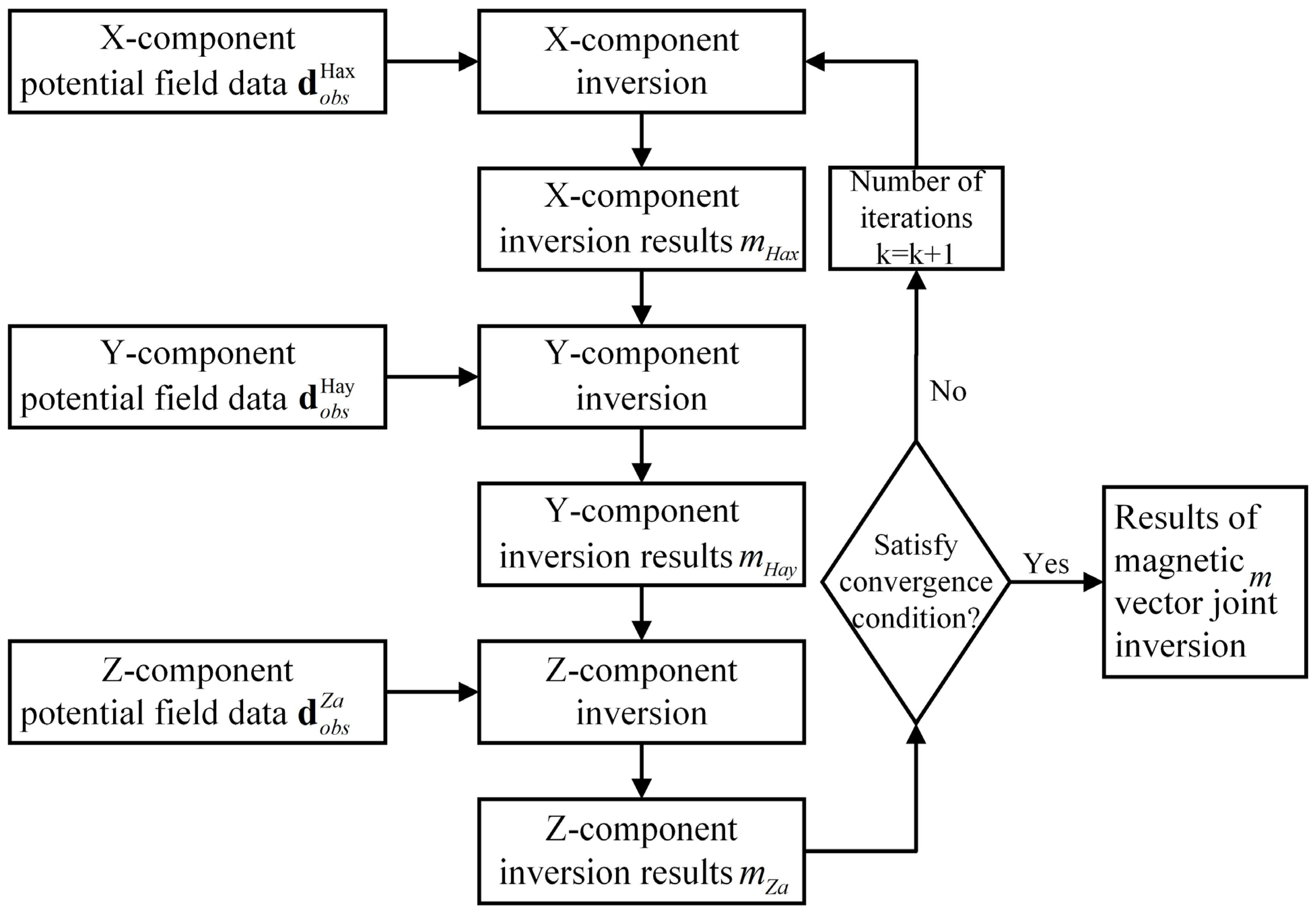
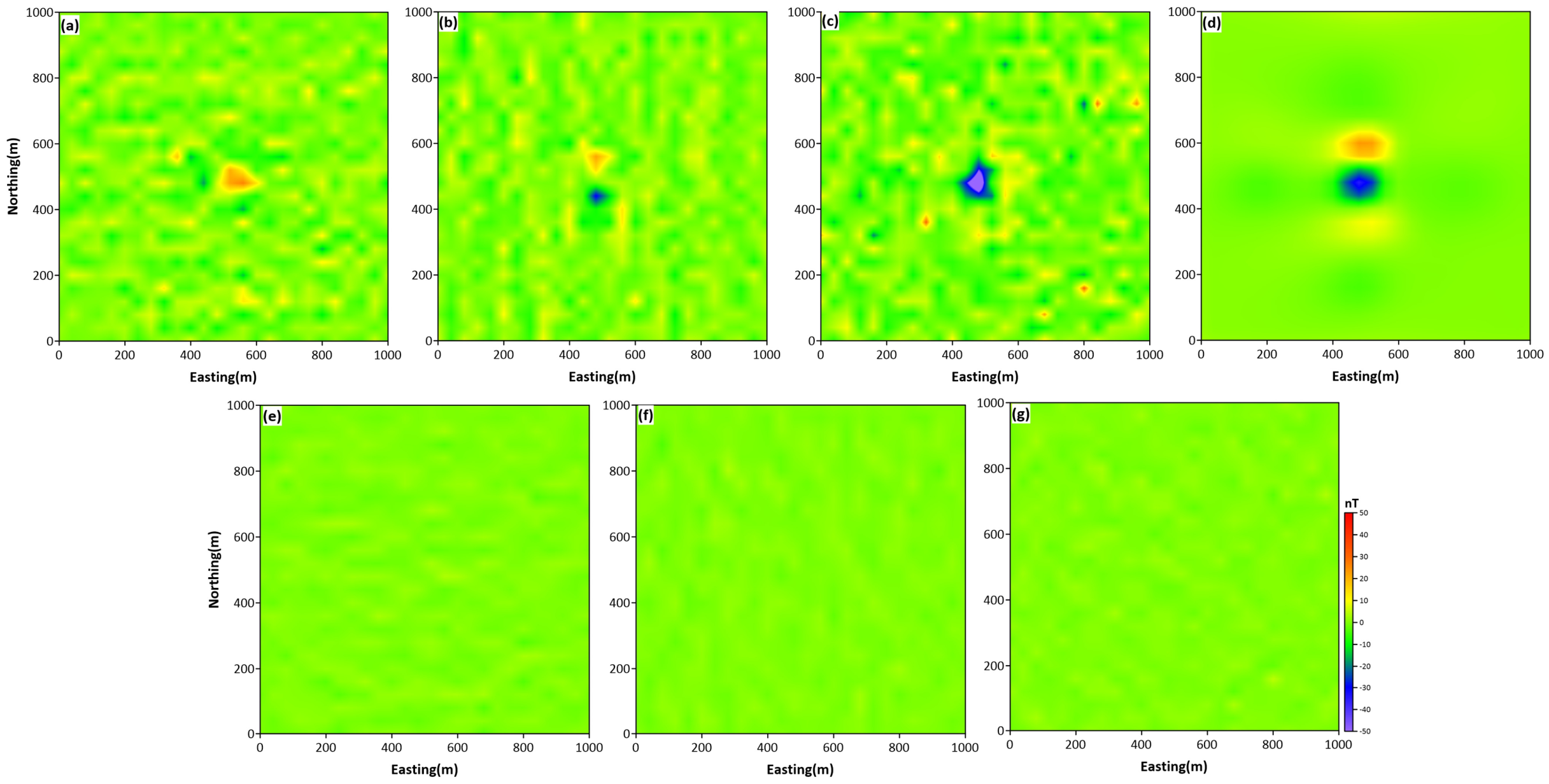
In this section, three sets of model experiments are designed to systematically analyze, from a numerical simulation perspective, the characteristic responses revealed by vector-data inversion results and to verify the effectiveness of the proposed joint inversion algorithm.

Specifically, Tests 1 and 2 investigate the potential field vector inversion characteristics under different strike and burial-depth conditions, respectively, using magnetic data as an example. Test 3 further constructs a comprehensive model and includes both magnetic and gravity vector tests to evaluate the general applicability of the proposed joint inversion strategy. In addition, conventional total-field inversion methods are implemented for comparison.

3.1. Test 1: Horizontal Feature Analysis

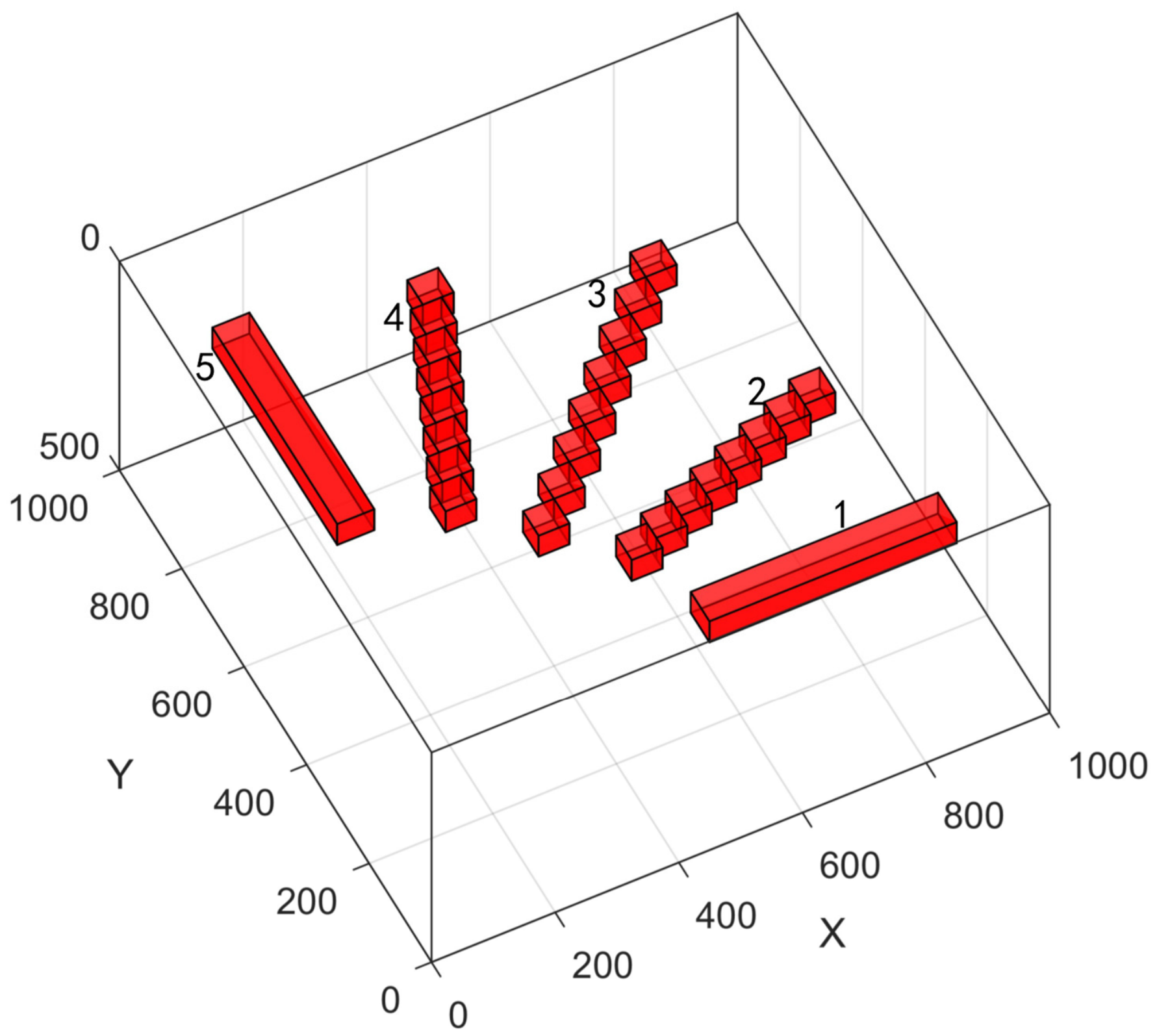
To evaluate the characterization capability of different magnetic vector data inversion methods for horizontally oriented anomalous bodies, this study designs a theoretical model comprising five prisms with distinct orientations. As shown in Figure 2, the prisms are oriented along horizontal directions of 0°, 25°, 45°, 65°, and 90°, while maintaining consistent geometric dimensions, burial depths, and magnetization intensities. Detailed physical-property parameters and spatial distribution information are provided in

Table 1. Spatial parameters and physical properties of the horizontal-strike model.

Block	1	2	3	4	5
Center coordinates (m)	(700, 130)	(625, 320)	(525, 525)	(320, 625)	(130, 700)
Magnetic susceptibility (SI)	0.05	0.05	0.05	0.05	0.05
Burial depth (m)	100–150	100–150	100–150	100–150	100–150

. To evaluate the robustness of the algorithm, 2% random noise is added to the model data. This model is employed to simulate common horizontally oriented structures encountered in actual geological settings. By comparing the spatial resolution and shape recovery capability of magnetic vector inversion results under different orientation conditions, the sensitivity and limitations of each component data inversion method to structural orientation are revealed.

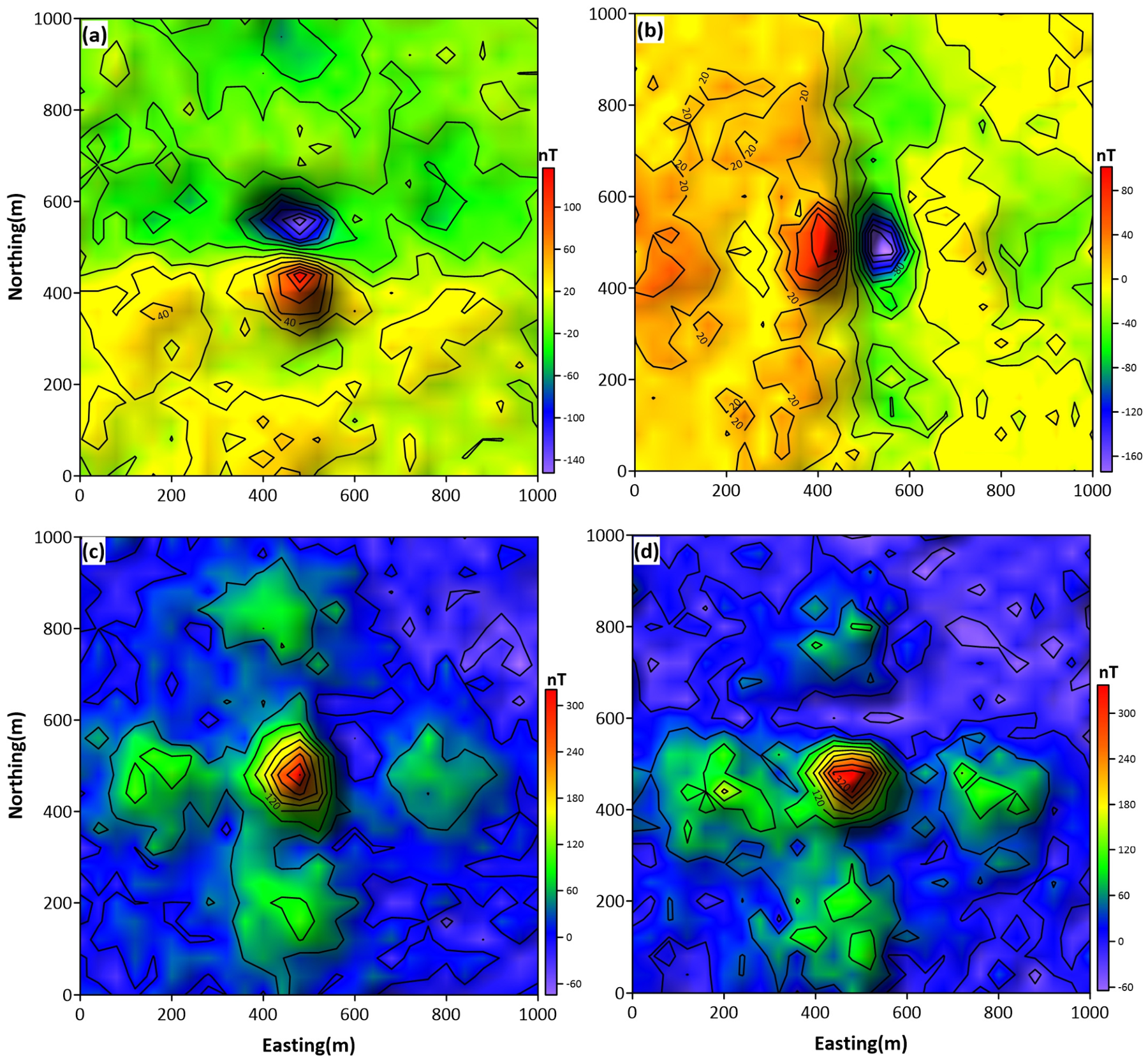
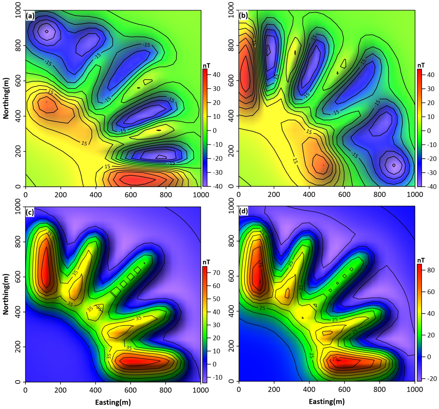
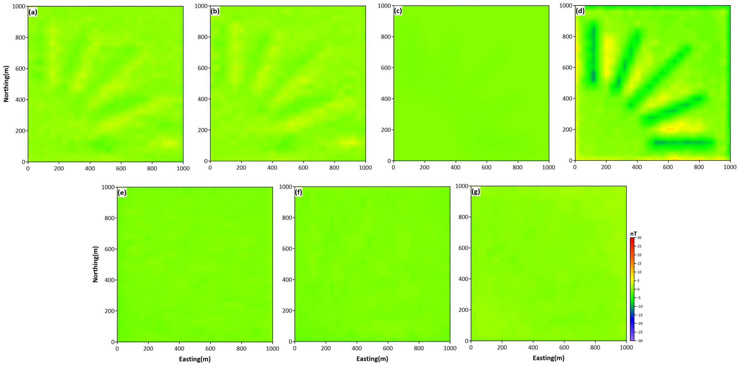
To simulate the actual geomagnetic environment, the background field intensity is set to 50,000 nT, with the magnetic inclination and declination set to 60° and 45°, respectively. On this basis, forward modeling of magnetic vector data and total magnetic field data is performed for the model. The results are shown in Figure 3, exhibiting distinct component-dependent response characteristics.

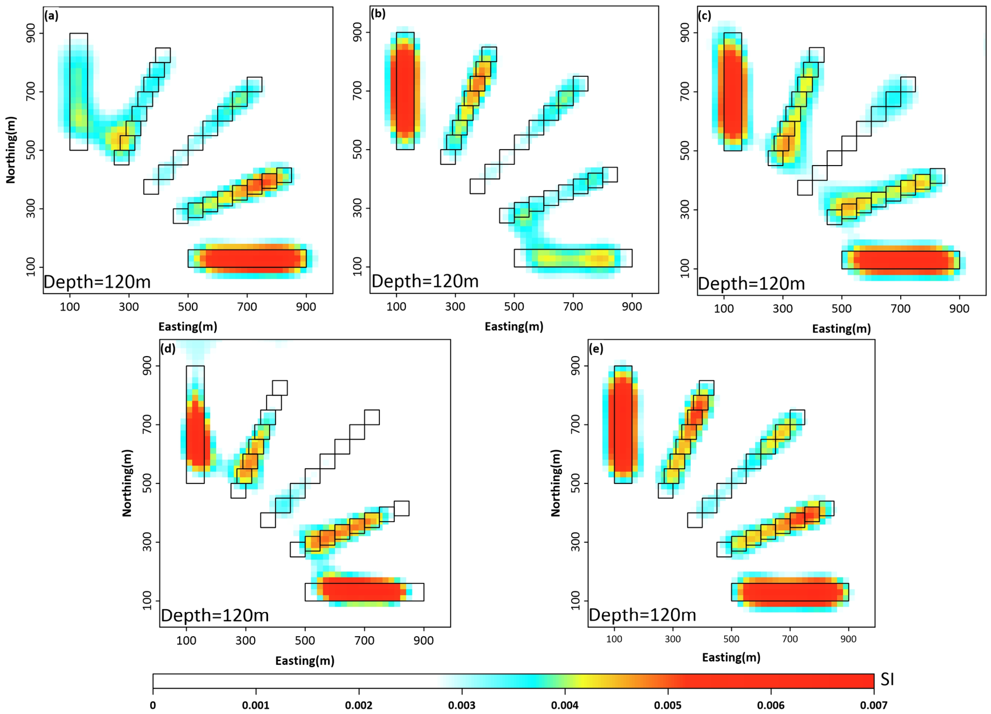
Based on the aforementioned forward-modeling theoretical data, magnetic vector inversion, magnetic vector joint inversion, and conventional total magnetic field inversion are performed. The inversion domain spans an area of 1000 m × 1000 m horizontally and extends to a depth of 500 m. It is discretized into 50 grids along the easting, northing, and vertical directions, resulting in a total of 125,000 regular cells with dimensions of 20 m × 20 m × 10 m. The inversion results are presented in Figure 4.

Figure 4a–c present the horizontal slice inversion results of the single-component magnetic vector inversion at a depth of 120 m. All three results clearly reveal five main high-magnetic anomalous bodies. Among them, the X-component inversion result most accurately characterizes Block 1, which extends along the X-direction; as the strike of the anomalous bodies gradually shifts toward the Y-direction, its characterization capability correspondingly weakens. The Y-component inversion result exhibits features complementary to those of the X-component, most clearly delineating the anomalous boundary of Block 5. Compared with the other two components, the Z-component provides relatively stable responses to the X- and Y-oriented end-member blocks, but its ability to recover obliquely striking bodies in the central part of the model is relatively limited. The above inversion results can effectively delineate the approximate location of the anomalous source, but there are significant differences among the inversion results from different vector data. When characterizing models with different orientations, these results exhibit clear complementarity, while each also demonstrates inherent limitations.

In parallel, this study further conducts total magnetic intensity data inversion and magnetic vector joint inversion experiments. Figure 4d presents the inversion results of the total magnetic intensity data; although this method can identify five distinct magnetic sources, their spatial distribution deviates to some extent from the preset model, with relatively blurred anomaly boundaries, insufficient lateral resolution, and notably weaker characterization of Block 3. In comparison, the magnetic vector joint inversion effectively integrates the response characteristics of each component, significantly enhancing the overall characterization capability for sources of different orientations. The resulting sources exhibit clearer boundaries and higher lateral resolution, and compared with total magnetic field inversion, the joint inversion more accurately delineates the contours of the sources and recovers their complete morphology.

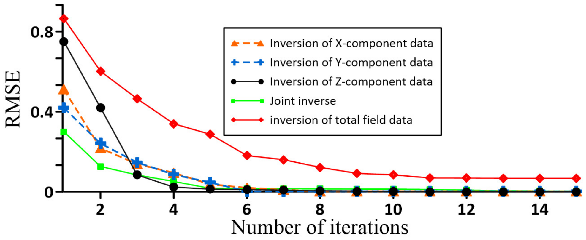
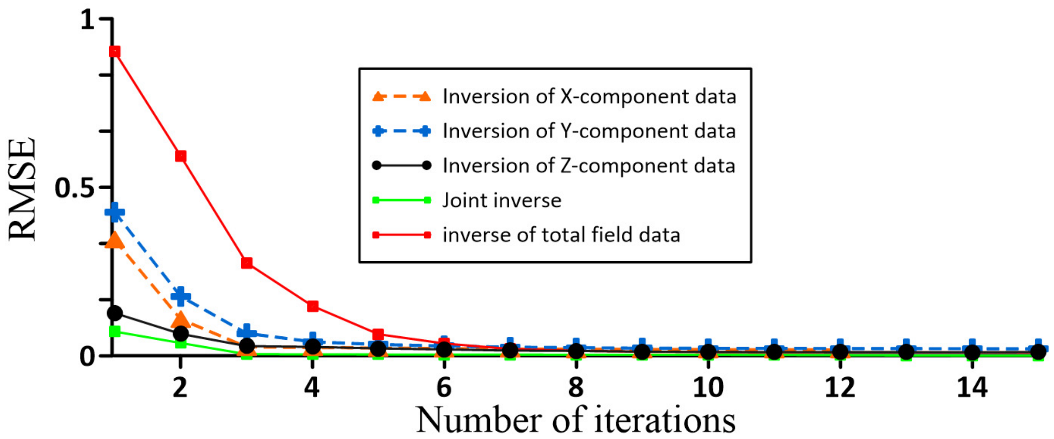
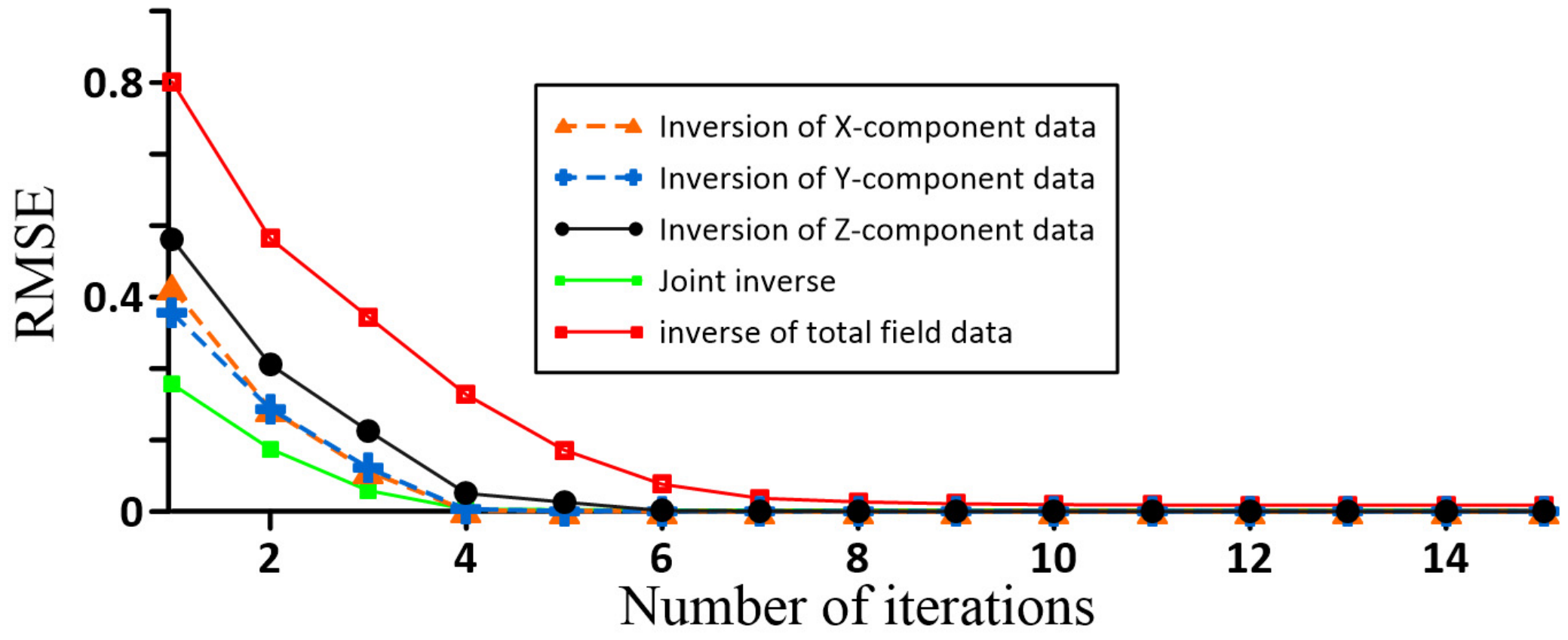
By comparing the iterative fitting curves (Figure 5) and data residual distributions (Figure 6), it can be seen that the proposed magnetic vector joint inversion method achieves faster convergence and higher fitting accuracy. Figure 5 shows that the RMSE of the joint inversion decreases rapidly within fewer iterations and then becomes stable, with a final error lower than those of the single-component and total-field data inversions. The data errors of all inversion methods become essentially stable after the eighth iteration. Figure 6 further shows that the residuals of each component after joint inversion have lower amplitudes and more uniform distributions, whereas the total-field data inversion still exhibits obvious structured residuals. These results indicate that the proposed method can effectively integrate multicomponent information, reduce data residuals, and improve the reliability of the inversion results.

The comparison of different inversion results shows that single-component inversion exhibits clear directional dependence: the X- and Y-components are most sensitive to sources extending along their respective axes, whereas the Z-component can identify sources oriented along the X- and Y-directions but has limited ability to recover the morphology of oblique anomalous bodies. Conventional total-field magnetic inversion can identify multiple anomalous bodies, but the recovered boundaries are blurred and the lateral resolution is insufficient. In contrast, magnetic vector joint inversion integrates multi-component information, reduces the directional dependence of single-component inversion, and more accurately recovers the boundaries, morphology, and horizontal spatial distribution of geological bodies with different strikes.

3.2. Test 2: Vertical Characteristic Analysis

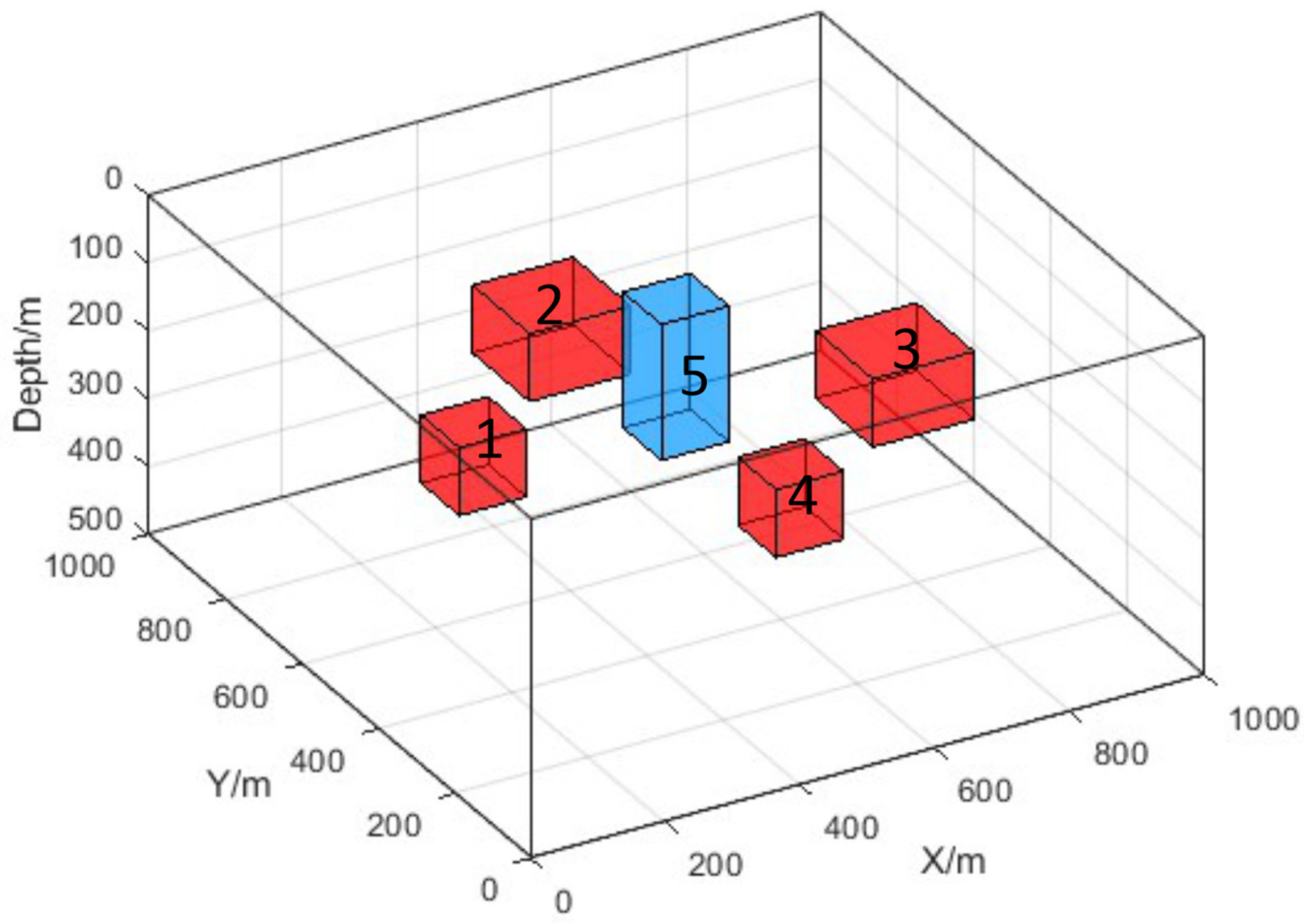
To evaluate the performance of different magnetic vector inversion methods in characterizing vertical sources, a composite model featuring five theoretical prisms is designed, as shown in Figure 7. These prisms vary in their top depth, dimensions, and vertical extent, with their specific physical parameters and spatial distribution detailed in

Table 2. Position and physical properties table for different depths model experiments.

Block	1	2	3	4	5
Center point coordinates (m)	(200, 500)	(500, 800)	(800, 500)	(500, 200)	(500, 500)
Magnetic susceptibility (SI)	0.1	0.1	0.1	0.1	0.05
Block burial depth (m)	150–250	200–300	200–300	150–250	50–250

. To evaluate the robustness of the algorithm, 8% random noise is added to the model data. A comparative analysis of the spatial resolution and shape recovery capabilities of the inversion results reveals the distinct influence of each magnetic vector component on the fidelity of vertical structure reconstruction.

For the above model, the background field is set with an intensity of 50,000 nT, an inclination of 45°, and a declination of 60°. Forward modeling is performed for both magnetic vector data and total magnetic field data, with the results shown in Figure 8. The forward-modeled data exhibit distinct component-dependent response characteristics. Based on these data, magnetic vector inversion, magnetic vector joint inversion, and conventional total magnetic field inversion are carried out. The inversion domain and mesh discretization settings remain the same as those in Model Experiment 1, and the model inversion results are presented as slices in Figure 9.

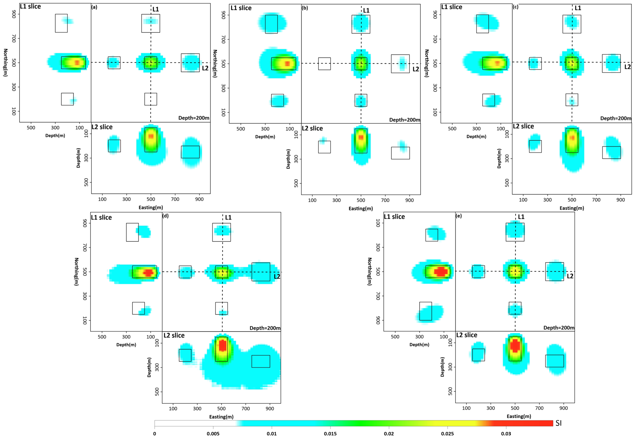
The analysis of the inversion results based on the X, Y, and Z components (Figure 9a–c) indicates that different components exhibit distinct capabilities in characterizing anomalous bodies with specific orientations: the X component provides more accurate depth characterization for Blocks 1, 5, and 3 aligned along the X-direction; the Y component offers clearer delineation of the top and bottom boundaries for Blocks 2, 5, and 4 oriented along the Y-direction; while the Z component presents a relatively complete depiction of the vertical distribution characteristics of all five major anomalous bodies. Overall, each component has its own features in terms of boundary delineation, positional correspondence, and depth resolution, reflecting both the complementary strengths and inherent limitations of multi-component data in inversion applications.

Compared with single-component magnetic vector inversion, both total-field magnetic inversion and magnetic vector joint inversion provide a more comprehensive representation of the source information. Figure 9d presents the inversion results based on total magnetic intensity data. Although all five main anomalous bodies are discernible, the boundary between Block 5 and Block 3 is blurred. In the vertical slices, the L2 profile locates Block 1 relatively well; however, the boundaries of Block 5 and Block 3 remain poorly defined and deviate from the preset model. In the L3 profile, Block 2 and Block 4 appear shallower than their actual positions, and Block 5 exhibits poor vertical resolution with a downward smearing of the anomaly. In contrast, the magnetic vector joint inversion results (Figure 9e) display clearly defined boundaries and complete morphology for all anomalous bodies in the horizontal slices. The vertical slices show sharper boundary delineation, more accurate spatial positioning, and higher fidelity in property recovery. Overall, the joint inversion demonstrates significant improvement compared to both single-component and total-field magnetic inversions.

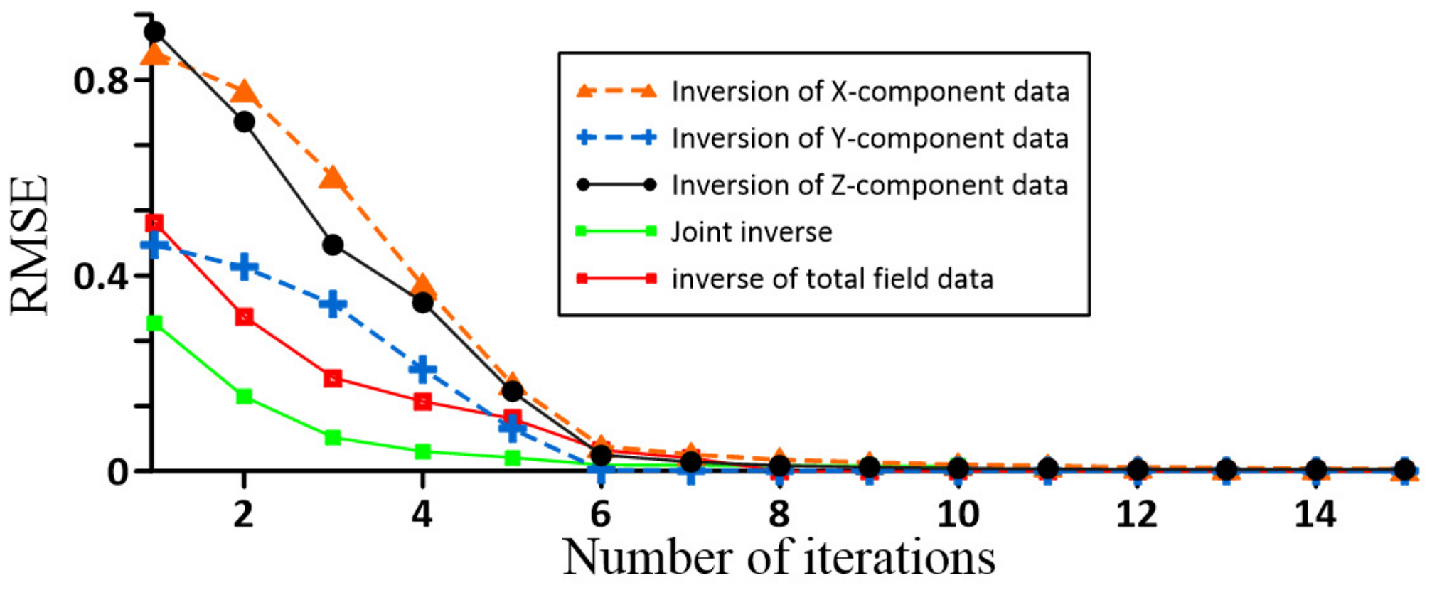
Figure 10 shows that, after random noise was added, the RMSE values of all inversion methods gradually decreased with increasing iteration number and then became stable. Among them, the magnetic vector joint inversion maintained a lower final error, indicating good convergence stability. The data errors of all inversion methods become essentially stable after the sixth iteration. Figure 11 shows that the residuals of the single-component inversions and total-field data inversion are mainly concentrated in the central part of the model, with the total-field data residuals showing particularly distinct positive and negative anomaly concentrations. In contrast, the residuals of each component after joint inversion have smaller amplitudes and more uniform distributions, indicating that the proposed method can effectively suppress local residual anomalies and improve data fitting under noisy conditions.

Based on experimental analyses of models at varying depths, it is observed that the X-component data more accurately determines the depth of blocks aligned along the X-direction, while exhibiting a weaker response to sources from blocks aligned along the Y-direction at greater burial depths. The Y-component inversion results show a similar orientation dependence. In contrast, the Z-component inversion enhances the overall characterization of both shallow and deep anomalous bodies. By integrating the advantages of each component, the magnetic vector joint inversion algorithm achieves higher accuracy in locating block centers and demonstrates better fidelity in physical-property recovery.

3.3. Test 3: Comprehensive Characteristic Analysis

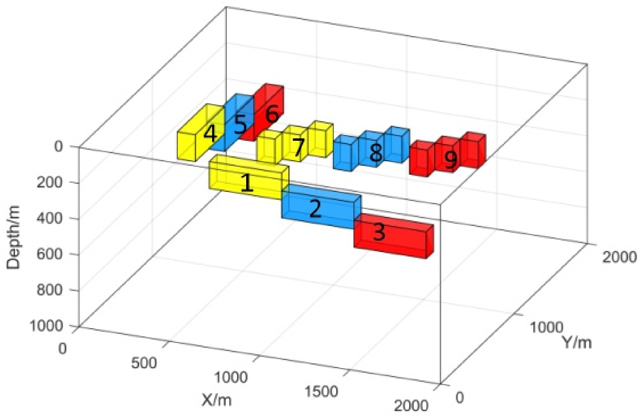
This set of tests further constructs a comprehensive block model, which accounts for variations in both orientation and burial depth. By simultaneously incorporating different orientations and multiple depth distributions, the model enables the simultaneous evaluation of the inversion method’s ability to identify and locate source bodies with distinct orientations and burial depth characteristics. The schematic diagram of the model is shown in Figure 12, and the specific parameters are listed in

Table 3. Position and physical properties table for synthetic block magnetic model experiments.

Block	1	2	3	4	5	6	7	8	9
Center point coordinates (m)	(800, 350)	(1200, 350)	(1600, 350)	(350, 800)	(350, 1200)	(350, 1600)	(850, 850)	(1050, 1050)	(1250, 1250)
Magnetic susceptibility (SI)	0.04	0.08	0.15	0.04	0.08	0.15	0.04	0.08	0.15
Block depth (m)	100–250	200–350	300–450	100–250	200–350	300–450	100–250	200–350	300–450

.

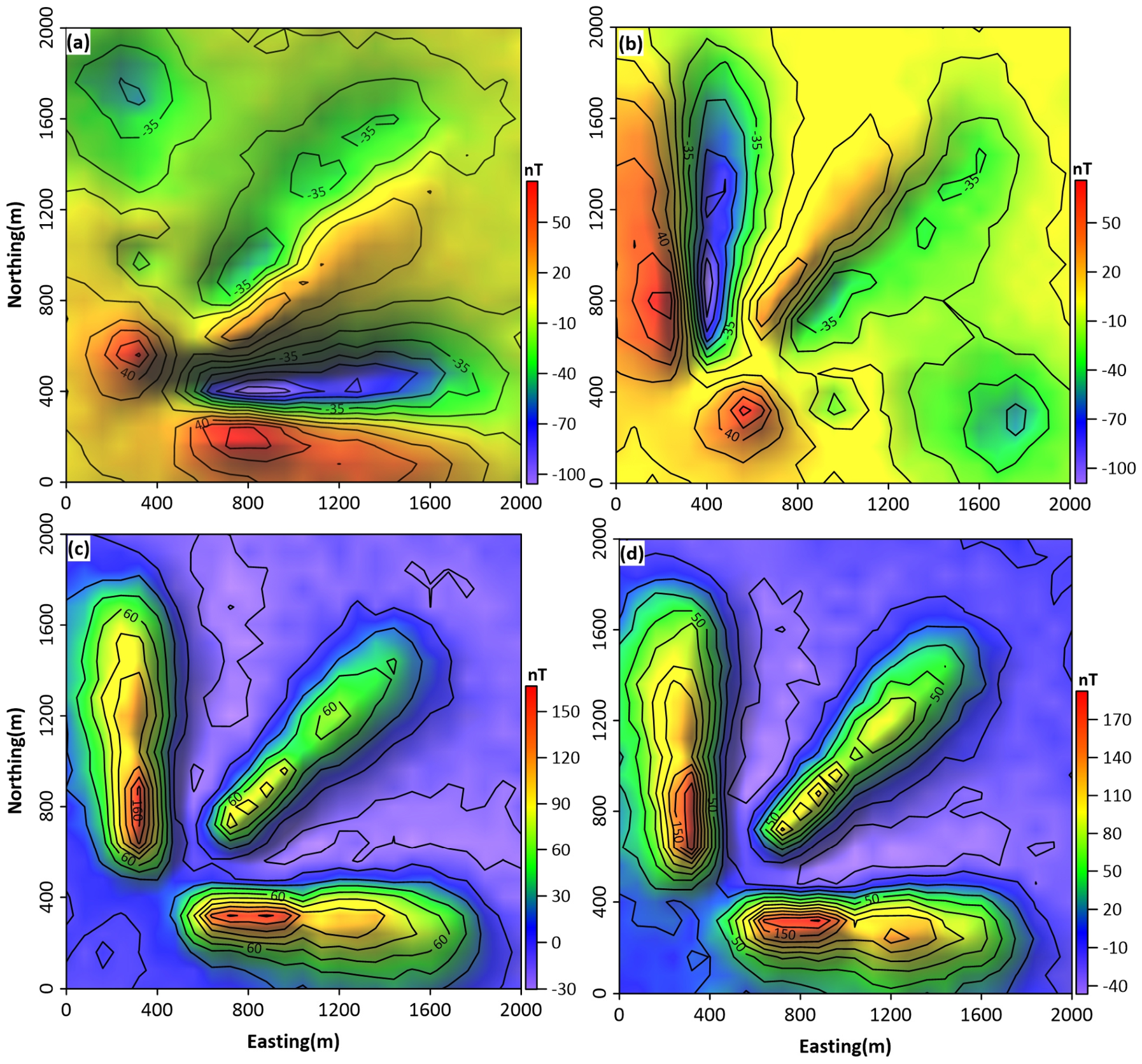
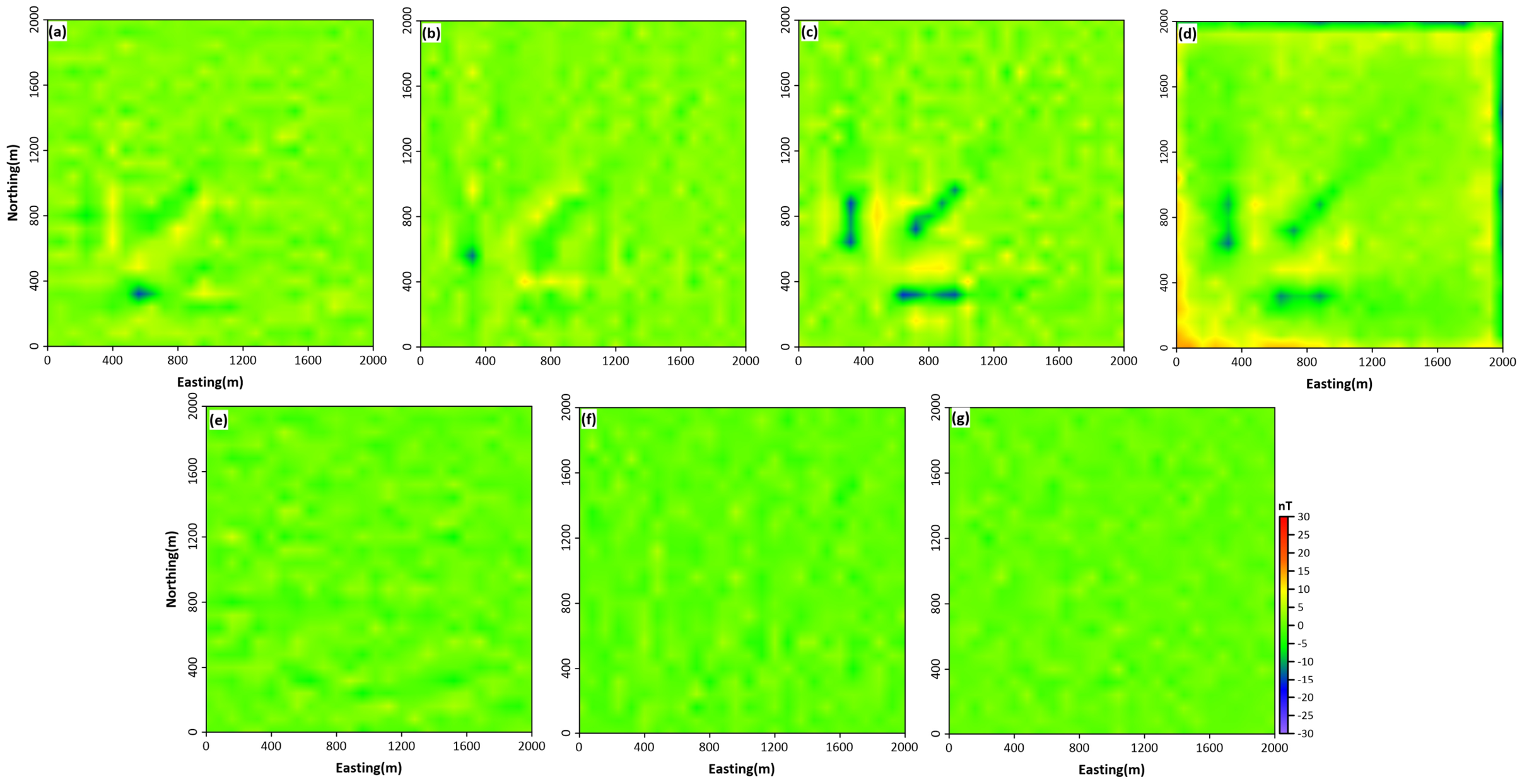
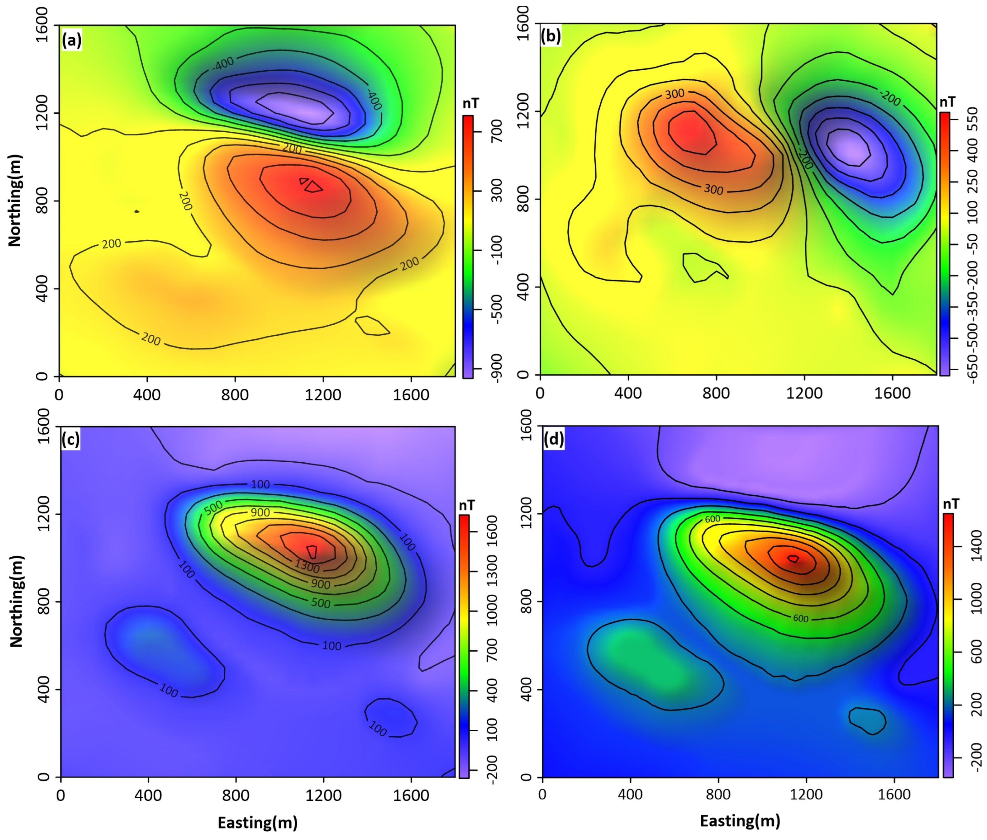
The model is situated in a geomagnetic field with an intensity of 50,000 nT, an inclination of 45°, and a declination of 45°. During the forward modeling, 3% random noise is added to the forward-modeled data to better approximate actual observational conditions. The forward modeling results are presented in Figure 13.

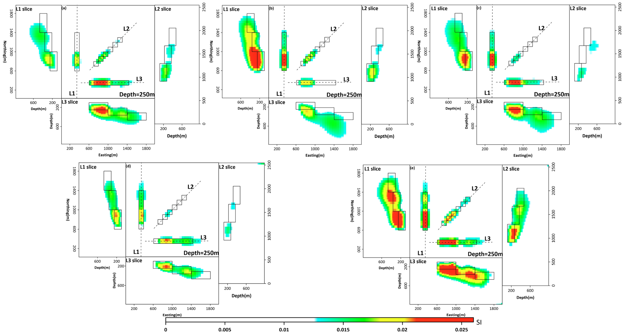
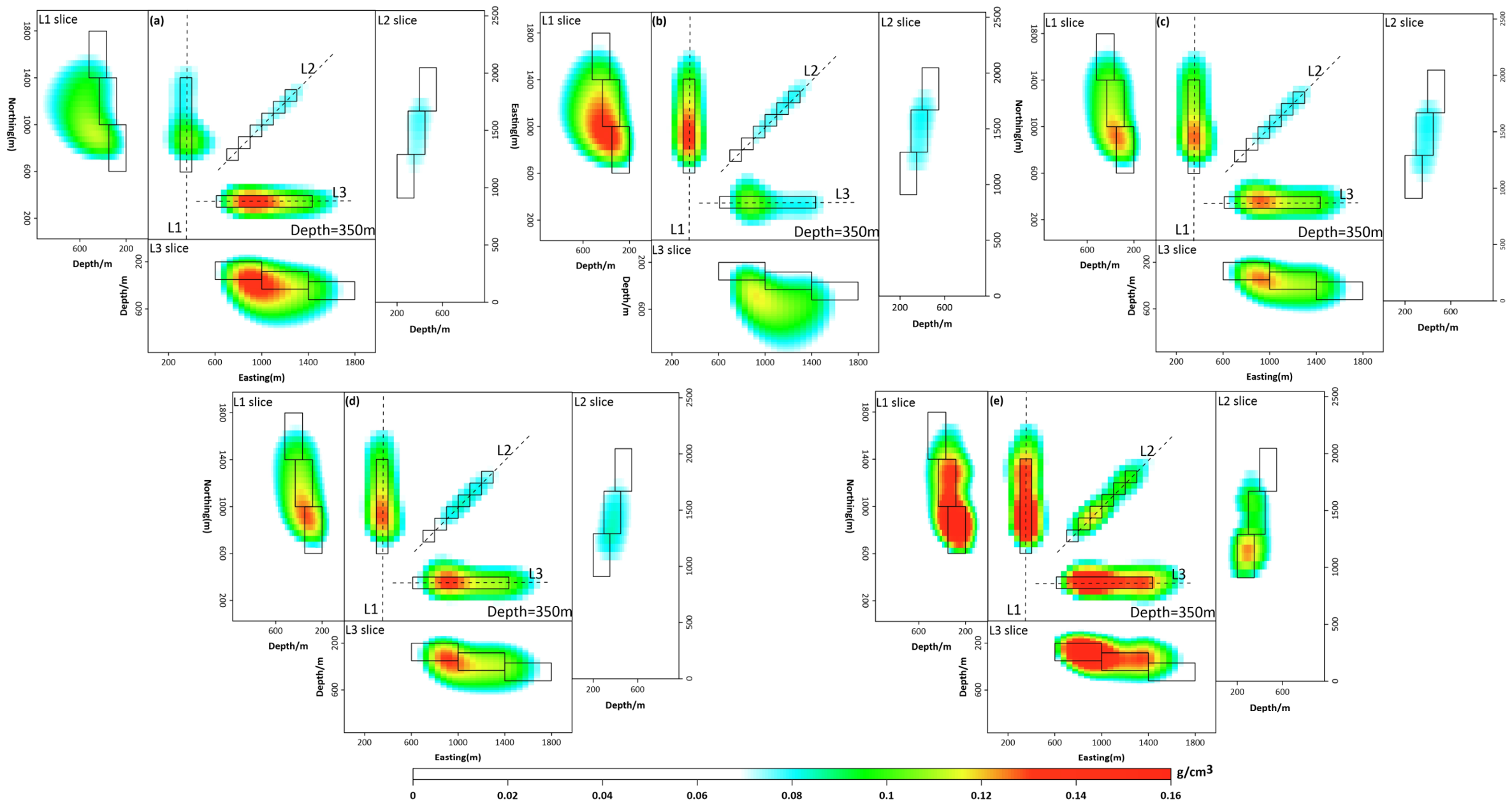
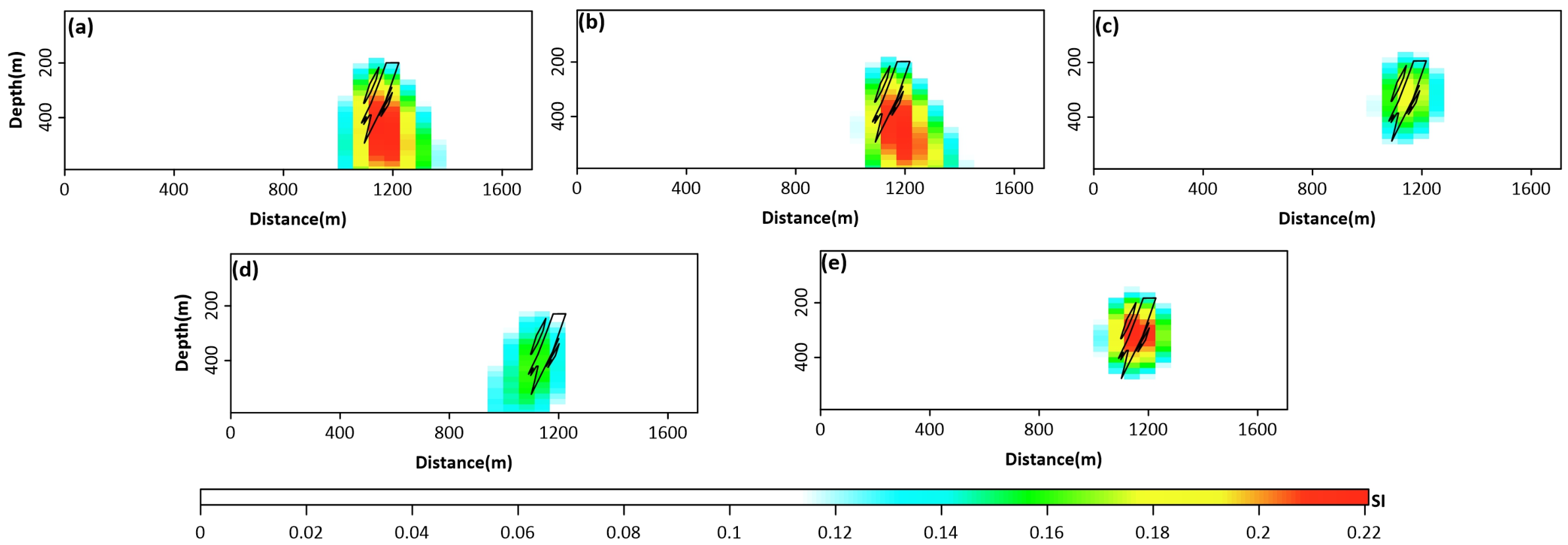
Following the experimental procedure described above, this study performs magnetic vector data inversion, total magnetic intensity data inversion, and magnetic vector joint inversion on the model. The inversion domain spans an area of 2000 m × 2000 m horizontally and extends to a depth of 1000 m. It is discretized into 40 grids along the easting and northing directions, and into 50 grids along the vertical direction, resulting in a total of 80,000 regular cells with dimensions of 40 m × 40 m × 50 m. The corresponding inversion results are presented in Figure 14.

Figure 14a–c present the inversion results of the X-, Y-, and Z-components, respectively. The horizontal slices show that the X-component provides relatively accurate positioning for models extending along the X-direction but yields a blurred delineation of blocks extending along the Y-direction. The Y-component accurately locates models extending along the Y-direction, while its response to models oriented along the X-direction is relatively weak. The Z-component delineates the positions of ore bodies extending in both the X- and Y-directions quite well, though its characterization capability for the central part of the ore body is limited. The vertical profiles reveal that the X-component produces the most accurate anomaly delineation on the L3 profile, whereas the representation of deeper blocks on the L1 profile shows deviations. In the Y-component inversion results, the L1 profile provides the best anomaly delineation, but the L3 profile exhibits significant positional errors. The Z-component yields relatively accurate anomaly characterization on both the L1 and L3 profiles, while on the L2 profile the sources are severely distorted. In summary, the inversion results of each component show clear differences and limitations in terms of anomaly positioning accuracy, boundary continuity, and deep recovery capability.

In parallel, this study conducts total-field magnetic inversion and magnetic vector joint inversion calculations. The corresponding results are presented in Figure 14d,e. Figure 14d presents the inversion results based on total magnetic intensity data. The horizontal slices show clear boundaries and good spatial correspondence for the X- and Y-oriented models, but the response to the central model block is weak, with scattered sources. On the vertical profiles, while the L1 and L3 profiles can reflect the orientation of the anomalous bodies, they inadequately characterize the deeper blocks. The L2 profile, however, exhibits significant deviations in the number and position of sources, along with severe morphological distortion. In contrast, the magnetic vector joint inversion results proposed in this study (Figure 14e) provide a more complete recovery of the boundary morphology and spatial distribution of anomalous bodies with different orientations. Particularly for the central anomalous block model, the anomaly responses are more continuous and closer to the theoretical model. In the vertical profiles, the amplitude and spatial distribution of the recovered property values align more closely with the true model, significantly enhancing the characterization capability for deeper blocks, with sharper boundaries.

In the comprehensive model experiments, the component data of each exhibits distinctly different response characteristics in both horizontal and vertical directions. Although total magnetic intensity data can reflect the overall trend of anomalous bodies to some extent, its ability to characterize deeper ore bodies is limited, with signals decaying significantly with depth. The magnetic vector joint inversion method effectively integrates the characteristics of each component dataset, enabling accurate identification of anomalous blocks distributed at different depths and orientations, and the physical-property values obtained from the inversion are closer to the preset model values.

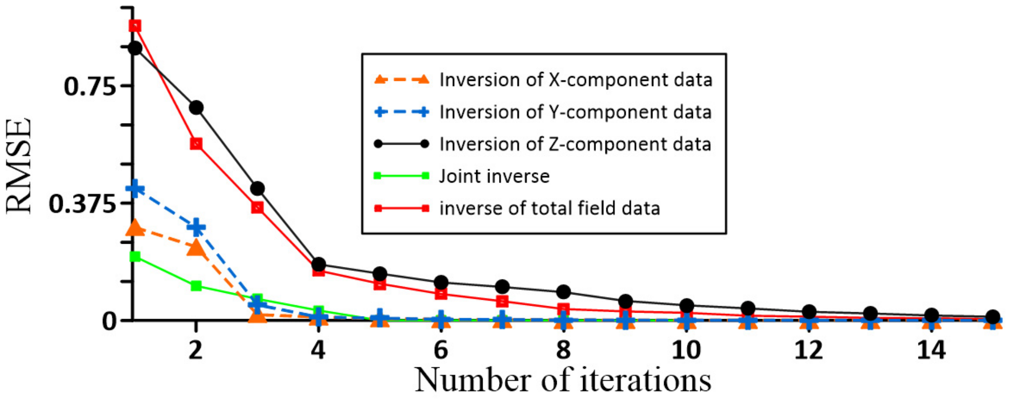
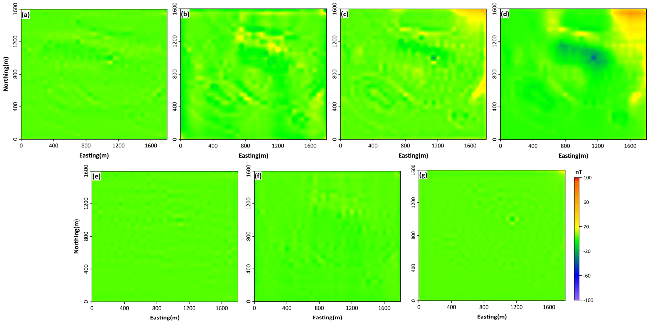
Figure 15 and Figure 16 show the iterative error variation and data residual distributions of different inversion methods, respectively. As shown in Figure 15, the RMSE values of all inversion methods decrease rapidly during the first few iterations and become essentially stable after the sixth iteration, with the magnetic vector joint inversion achieving a relatively lower final error. Figure 16 indicates that local residual anomalies remain in the single-component inversions and total-field data inversion, whereas the residuals of each component after magnetic vector joint inversion have overall smaller amplitudes and more uniform distributions, suggesting that the proposed method can effectively reduce data residuals and improve the fitting performance.

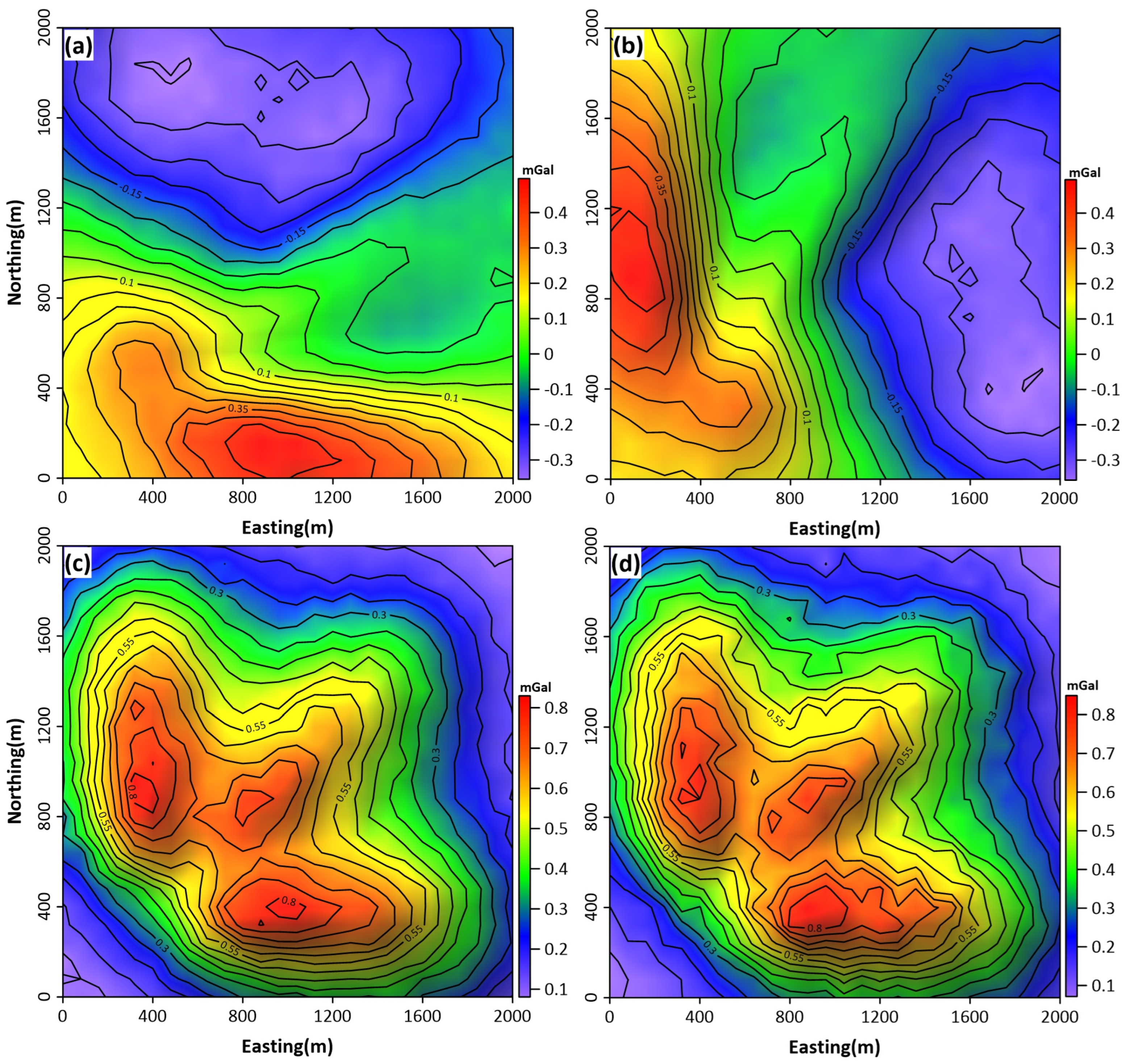
To further examine whether the component-response characteristics observed in magnetic inversion are also applicable to gravity vector data, this study constructs a density model with a geometry similar to that of the comprehensive magnetic model and conducts gravity vector inversion tests. The detailed geometrical and physical-property parameters of this are listed in

Table 4. Position and physical properties table for synthetic block of density model experiments.

Block	1	2	3	4	5	6	7	8	9
Center coordinates (m)	(800, 350)	(1200, 350)	(1600, 350)	(350, 800)	(350, 1200)	(350, 1600)	(850, 850)	(1050, 1050)	(1250, 1250)
Density (g/cm3)	0.04	0.08	0.15	0.04	0.08	0.15	0.04	0.08	0.15
Burial depth (m)	200–350	280–430	370–520	200–350	280–430	370–520	200–350	280–430	370–520

. To better simulate real world conditions, 5% Gaussian random noise is added to the theoretical noise-free data. The gravity anomalies are demonstrated in Figure 17. The inversion domain and mesh discretization are consistent with those in Experiment 3. The inversion results are shown in Figure 18.

Figure 18a–c show the inversion results obtained from the x-, y-, and z-components of the gravity data, respectively. The sections show that the x-component inversion preferentially recovers the horizontal body extending along the L3 direction, but gives a weak response to the oblique body along the L2 direction and exhibits obvious distortion for the block extending along the L1 direction. Similar to the x-component inversion result, the y-component inversion result has poorer depth resolution. It provides a more accurate delineation of the block in the L1 direction, but shows obvious distortion for the block in the L3 direction, and the recovery of the block striking L2 is relatively weak. In comparison, the z-component inversion exhibits more uniform sensitivity to source with different orientations, producing a closer spatial correspondence with the prescribed model and improved boundary continuity. Even so, the deeper part of the model remains affected by amplitude attenuation and local smearing.

For comparison, conventional gravity inversion and the gravity vector joint inversion are also performed, and the results are shown in Figure 18d,e. The conventional gravity inversion result in Figure 18d is similar to that of the z-component inversion and agrees well with the location of the prescribed model, but it incompletely delineates the obliquely striking L2 block, with some anomalies missing. By contrast, the joint gravity vector inversion result in Figure 18e provides a more complete reconstruction of the geometry and spatial distribution of sources with different orientations. In particular, the oblique body along L2 and the deeper target are recovered with improved continuity and with locations that more closely match the true model. The vertical sections likewise show that the recovered density contrasts are in better agreement with the prescribed model in both amplitude and spatial extent, with sharper boundaries and improved resolution at depth.

Overall, the results show that inversion based on any single gravity component captures only part of the model response, owing to the directional sensitivity of the data. Conventional gravity anomaly inversion reproduces the general pattern of the sources but remains limited in its recovery of deeper and geometrically complex bodies. By combining the complementary information contained in the three gravity components, the gravity vector joint inversion yields a more reliable reconstruction of anomaly position, morphology, and depth extent, and produces density-contrast estimates that are closer to the true values.

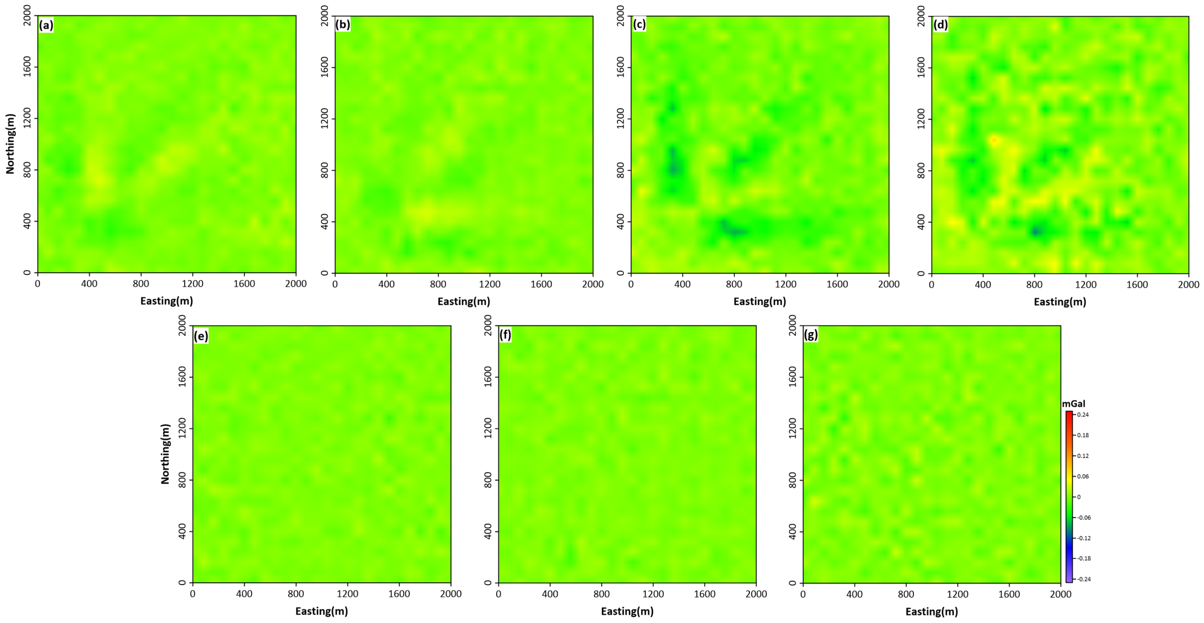
An iteration performance curve (Figure 19) shows that the total-field data inversion and Z-component inversion have relatively high initial RMSE values and exhibit slower decreases during the iteration process. In contrast, the joint inversion maintains a lower error throughout the iterations and rapidly reaches a stable state. Data residual maps (Figure 20) indicate that local blocky or banded anomalies remain in the residuals of the single-component and total-field inversions, mainly distributed in the central part of the model. By comparison, the residual amplitudes after joint inversion are significantly reduced, the spatial distribution becomes more uniform, and the local anomalies are effectively weakened. Overall, the gravity vector joint inversion improves the data fitting performance and enhances the stability of the density model inversion results.

Based on the three sets of model experiments, the component-dependent characteristics of potential field vector inversion are further confirmed. The X-component provides the best delineation of sources extending along the X-direction, but its delineation capability decreases as the source strike gradually rotates toward the Y-direction. The Y-component exhibits the opposite response pattern. The Z-component provides relatively stable spatial positioning and improves vertical resolution, but its ability to recover physical-property contrasts remains limited. By integrating the complementary information from individual components, the proposed potential field vector joint inversion method improves horizontal positioning accuracy, vertical resolution, boundary recovery, and physical-property reconstruction, demonstrating superior inversion performance for sources with complex variations in strike and burial depth.

4. Real Data Application

The Galinge iron deposit is situated near Golmud City in Qinghai Province, China, within the Qimantage metallogenic belt, where it represents the largest skarn-type deposit. The local topography is relatively flat, with bedrock concealed beneath Quaternary gravel sediments ranging from 117 to 210 m in thickness. Numerous economically significant deposits have been discovered in this belt over recent decades. The ore cluster examined in this study is located on the northern limb of a syncline in the eastern section of the deposit [32,33]. The mining area trends WNW, extending approximately 1.6 km in length and 0.8 km in width. Total magnetic intensity contour maps of the region reveal a prominent, regularly shaped magnetic high, exhibiting an ellipsoidal form elongated in a NW-SE direction, with an amplitude exceeding 1600 nT. Multiple boreholes with measured data have been obtained within this area, providing a reliable basis for validating the inversion results [33].

In the study area, the geomagnetic inclination is 56°, the declination is 4°, and the total geomagnetic field intensity is 53,800 nT. Although the rocks in the region possess a certain degree of remanent magnetization, its intensity is weak, and its direction is largely consistent with that of the current geomagnetic field. Based on the aforementioned geomagnetic parameters, a component transformation was performed on the measured total magnetic field anomaly data, yielding the X, Y, and Z components of the magnetic anomaly for the area, as shown in Figure 21. As shown in Figure 21a, the X-component magnetic anomaly exhibits a distinct spatial distribution characterized by “negative in the north and positive in the south,” with its anomaly center largely coinciding with the known ore body locations. The Y-component anomaly displays an “east-positive and west-negative” pattern, reflecting clear directional component characteristics. The Z-component data is shown in Figure 21c, revealing a primary positive magnetic anomaly in this area that is broadly consistent with the location of the known ore body.

Single-component magnetic vector inversion, total-field magnetic inversion, and magnetic vector joint inversion are performed using the above data. The inversion results obtained by each method are sliced along the A–B profile, and the corresponding profile sections are shown in Figure 22. The X-component inversion result (Figure 22a) can effectively identify the high-magnetic anomaly corresponding to the known ore body, but the anomaly extends downward to some extent and its lower boundary is relatively diffuse, indicating limited depth constraint. Similarly, the Y-component inversion result (Figure 22b) shows more pronounced downward diffusion of the high-value zone, with stronger deep smearing and an unclear lower boundary. The Z-component inversion result (Figure 22c) exhibits a more concentrated anomaly pattern and agrees well with the spatial position of the known ore body; however, the recovered physical-property values are generally low, indicating insufficient recovery of the high-magnetic core. The conventional total-field magnetic inversion result (Figure 22d) can reflect the approximate position of the anomalous body, but it has relatively low depth resolution and poor recovery of physical-property values. The magnetic vector joint inversion result (Figure 22e) shows the best agreement with the position and morphology of the known ore body. The high-value anomaly is mainly concentrated within the ore body, with clearer boundaries, better-constrained deep extension, and recovered physical-property values closer to the actual model. Overall, magnetic vector joint inversion outperforms both single-component inversion and conventional total-field magnetic inversion in spatial localization, boundary delineation, and physical-property recovery.

The iterative variation of RMSE during real-data inversion (Figure 23) shows that the fitting curve of the joint inversion method becomes essentially stable after the fourth iteration. Figure 24 shows the data residual distributions obtained from different inversion methods. Overall, the residuals from single-component data inversion (Figure 24a–d) still retain certain spatially structured features, with relatively pronounced positive and negative residual anomalies in local areas. This indicates that single-component data inversion remains insufficient in fitting the observed data. In particular, distinct banded or blocky residual patterns can be observed in the residuals of the Y-component, Z-component, and total-field magnetic inversion, with relatively prominent residuals in the central and northeastern parts of the study area. In contrast, the three-component residuals after magnetic vector joint inversion (Figure 24e–g) show a marked decrease in overall amplitude and a more uniform spatial distribution. Most areas are close to zero residual, with only weak local residual anomalies remaining. These results indicate that magnetic vector joint inversion can more fully fit the multi-component observations, effectively reduce the systematic residuals present in single-component inversion, and improve both data-fitting accuracy and the reliability of the inversion results.

This study conducted inversion experiments using magnetic vector data and magnetic vector joint inversion based on magnetic vector data from the Galinge area. The experimental results further reveal the response characteristics and limitations of each component in the inversion process, while validating the effectiveness and superiority of the magnetic vector joint inversion algorithm proposed in this paper in practical geological scenarios. By effectively integrating information from each component dataset, the algorithm fully leverages the complementary advantages of different components in delineating the orientation, boundaries, and depth of anomalous bodies, significantly improving the spatial positioning accuracy, boundary resolution capability, and physical-property recovery reliability of the inversion results.

5. Conclusions

In summary, this study reveals the differences and complementarity among potential field vector components in inversion through systematic modeling experiments. The results show that the X- and Y-components are more sensitive to sources extending along their corresponding directions, whereas the Z-component provides a relatively stable overall response but still has certain limitations in local resolution. Based on this understanding, this study proposes a sequential joint inversion algorithm for potential field vector data. By progressively integrating single-component inversion results, the method fully exploits the complementary information from different components, thereby improving the accuracy of anomaly localization, boundary delineation, and physical-property recovery. This provides a more reliable geophysical basis for identifying concealed ore bodies, finely delineating ore-body boundaries, and prioritizing mineral exploration targets.

Nevertheless, the computational efficiency of the proposed method in large-scale, high-resolution three-dimensional inversion and its applicability under complex geological conditions still require further improvement. Future work may incorporate fast algorithms such as wavelet compression to reduce the storage and computational costs of large-scale kernel matrices, enabling efficient three-dimensional inversion of high-density potential field vector data. Further studies should also explore adaptive component weighting, uncertainty assessment, and applications in complex geological settings to enhance the robustness and practicality of the method in mineral exploration.