Interpretable Machine-Learning-Assisted Analysis of Caustic Leaching for Purification of Spent Cathode Carbon

Abstract

Spent cathode carbon (SCC), a hazardous by-product generated during aluminum electrolysis, contains significant amounts of fluorides, cyanides, and other impurity phases that require effective purification before recycling or reuse. Caustic leaching is an important step in the purification of spent cathode carbon (SCC), but the nonlinear relationships between operating conditions and the carbon content of the caustic-leaching residue remain insufficiently quantified. In this study, an interpretable machine-learning (ML) framework was developed to quantitatively investigate the caustic leaching purification behaviour of SCC and evaluate the influence of key process variables on the carbon content of leaching residues. A dataset of 42 experimental observations was reconstructed from the published single-factor and Box–Behnken experiments reported by Yuan et al. The dataset describes the NaOH-based caustic-leaching stage and includes temperature, leaching time, liquid-to-solid ratio, alkali-related operating conditions, and stirring rate as input variables. Six ML algorithms, including GBDT, Random Forest, XGBoost, LightGBM, GBR, and CatBoost, were systematically evaluated. Among the evaluated models, CatBoost showed comparatively better predictive consistency in terms of testing-set R² (0.9604) and RMSE (0.4087). However, given the limited dataset size (n = 42), five-fold cross-validation revealed substantial performance variability (mean R² = 0.29 ± 0.59), underscoring the need for cautious interpretation. Therefore, the primary value of this study lies not in establishing a universally predictive model, but in demonstrating how SHAP analysis, when coupled with strict cross-validation, can extract meaningful process insights—specifically, the dominant roles of alkali concentration and liquid-to-solid ratio—even under small-data conditions. Overall, this study demonstrates the potential of interpretable ML as a complementary data-reanalysis tool for identifying model-attributed variable–response associations and prioritizing experimental variables for further validation in small-sample hydrometallurgical systems.

1. Introduction

Spent cathode carbon (SCC), a hazardous solid waste generated during aluminum electrolysis, contains considerable amounts of soluble fluorides, cyanides, and other toxic compounds that may cause serious environmental and health risks if improperly managed [1,2,3,4,5]. With the increasing emphasis on sustainable metallurgy and circular economy strategies, the detoxification and resource utilization of SCC have attracted growing attention in recent years [3,4,5]. Among the available treatment methods, caustic leaching has been widely recognized as an effective purification approach for removing impurity phases and improving the quality of recovered carbon materials [2,6,7,8]. The leaching process involves complex physicochemical interactions among dissolution reactions, mass transport behavior, and solid–liquid interfacial phenomena, which evolve concurrently rather than being governed by a single dominant mechanism. During leaching, the dissolution of impurity phases, diffusion of reactive species within the liquid phase, and interfacial reactions occurring at the solid surface collectively influence reaction kinetics and system stability. The coupled interplay of these processes ultimately determines impurity removal efficiency, leaching performance, and the physicochemical characteristics of the residual carbon, including its composition, surface properties, and structural integrity [7,8,9,10]. From a separation and purification perspective, the efficiency of impurity dissolution and selective retention of the carbon matrix are critical factors determining the subsequent reuse potential of SCC-derived carbon materials.

The purification performance of SCC leaching is strongly influenced by operational parameters such as temperature, leaching time, liquid-to-solid ratio, reagent concentration, and stirring intensity [9,10]. These variables are often highly coupled and may simultaneously affect reaction equilibrium, diffusion pathways, reagent accessibility, and transport kinetics within the heterogeneous leaching system. For example, liquid-to-solid ratio directly influences concentration gradients and mass transfer conditions, while reagent concentration governs the chemical driving force for impurity dissolution [7,11]. As a result, the SCC leaching process exhibits pronounced nonlinearity and interaction effects, making it difficult to establish reliable predictive relationships using conventional empirical approaches alone.

Traditionally, optimization of SCC purification processes has mainly relied on experimental design methods such as one-factor-at-a-time (OFAT), response surface methodology (RSM), and Taguchi-based approaches [11,12,13,14]. Although these methods provide useful guidance for evaluating process variables, they generally assume simplified polynomial relationships between operational parameters and process responses. Such approaches are typically based on simplified assumptions and therefore may not adequately capture the strong nonlinear coupling, and multivariate interactions present in complex leaching systems [15,16,17]. In particular, they often struggle to represent the coupled, non-additive effects among process variables, especially in systems where multiple physicochemical mechanisms operate simultaneously and interact across different spatial and temporal scales. Furthermore, their predictive capability is often restricted to the investigated experimental domain, limiting their applicability for broader process optimization and interpretation under varying operating conditions.

In recent years, machine-learning (ML) has emerged as a promising tool for modeling highly nonlinear and mechanism-coupled hydrometallurgical and separation systems due to its ability to capture complex relationships directly from experimental data without relying on predefined mechanistic equations. Unlike conventional modeling approaches, ML methods can effectively identify hidden patterns, variable interactions, and nonlinear dependencies within multivariate process systems [16,17,18,19,20]. Algorithms such as Random Forest, Gradient Boosting, XGBoost, and CatBoost have demonstrated strong predictive performance in mineral processing and leaching applications [17,18,19,20,21,22,23,24]. More importantly, the development of explainable artificial intelligence (XAI) techniques, particularly SHapley Additive exPlanations (SHAP), has enabled quantitative interpretation of feature contributions and interaction effects within ML models [23,25,26,27,28]. This provides an opportunity to bridge data-driven prediction with physicochemical understanding in complex leaching systems.

Several recent studies have explored ML applications in hydrometallurgical processes. Feng et al. [29] developed predictive models for metal leaching from spent LiFePO4 materials and demonstrated improved optimization efficiency compared with traditional approaches. Zhang et al. [24] applied ML to pyrolusite leaching and identified critical operational variables affecting leaching performance. Niu et al. [30] further integrated ML with experimental validation to analyze parameter effects during metal recovery from spent lithium-ion batteries. However, existing studies mainly focus on improving prediction accuracy, while the integration of interpretable ML with physicochemical understanding of SCC purification behavior remains limited. Despite recent advances in ML-assisted hydrometallurgical modelling, limited studies have quantitatively linked interpretable ML outputs with physicochemical mechanisms governing impurity removal and purification behaviour in SCC caustic leaching systems. In particular, the relationships between operational parameters, reaction equilibrium, and transport behavior in SCC caustic leaching systems have not yet been systematically investigated using interpretable ML approaches. A comparison of recent ML applications in hydrometallurgical and leaching systems is summarized in

Table 1. Comparison of recent ML applications in hydrometallurgical leaching systems and the novelty of the present study.

Study	System	ML Method	Dataset Size	Interpretability	Main Contribution	Limitation
Feng et al. [29]	Spent LiFePO4 leaching	ML models	Experimental dataset	Partial	Prediction and sustainability assessment	Limited mechanistic interpretation
Zhang et al. [24]	Pyrolusite leaching	ML algorithms	Experimental dataset	No	Identification of key process variables	Focused mainly on prediction accuracy
Niu et al. [30]	LIB metal recovery	ML	Collect experimental data sets	Partial	Process parameter analysis	Limited integration with physicochemical mechanisms
Kim et al. [20]	Copper slag leaching	Interpretable ML	Comprehensive Experimental Dataset	Yes	SHAP-based analysis of copper leaching	Different hydrometallurgical system
This study	SCC caustic leaching	CatBoost + SHAP	42 samples	Yes	Mechanistic interpretation of SCC leaching under limited-data conditions	Limited dataset size

. Previous studies have mainly focused on data-driven modelling of hydrometallurgical systems, whereas phenomenological approaches have traditionally provided mechanistic descriptions based on reaction kinetics and transport processes. For example, phenomenological leaching models have been widely developed based on chemical kinetics, mass transfer, and differential-equation formulations to quantitatively describe mineral dissolution behaviour [16,17,20].

Compared with these approaches, the present study does not aim to replace phenomenological modelling. Instead, following the complementary perspective discussed in previous studies [16,17], the proposed interpretable ML framework is intended to complement mechanistic approaches by identifying model-attributed variable–response associations and prioritizing variables for subsequent mechanistic and experimental investigation.

In this study, the published experimental dataset reported by Yuan et al. was systematically reanalyzed using interpretable ML methods. The analysis focuses on the NaOH-based caustic-leaching stage of SCC purification. Six ML models were comparatively evaluated to examine their ability to capture nonlinear relationships between the operating variables and the carbon content of the caustic-leaching residue. SHAP analysis was further employed to quantify the model-attributed contribution of individual variables and to identify the operating conditions most strongly associated with the predicted response.

The primary contributions of this work are: (i) reanalysis of a published small-sample experimental dataset describing the NaOH-based caustic-leaching stage of SCC purification using interpretable ML; (ii) comparative evaluation of six ML models under a small-data setting; (iii) assessment of model-attributed feature contributions using SHAP; and (iv) cautious interpretation of the data-driven relationships in relation to established caustic-leaching phenomena, while explicitly distinguishing model-derived associations from experimentally verified mechanisms.

2. Experimental Materials and Methodology

2.1. Dataset

The dataset used in this study was derived from the experimental work reported by Yuan et al. [31], which investigated the purification of SCC through a combined caustic leaching process. The SCC samples were collected from newly decommissioned aluminum electrolysis cells and subjected to crushing, grinding, sieving (<100 mesh), and drying prior to leaching experiments. In the original purification process, SCC underwent sequential caustic leaching and acid leaching. During the caustic-leaching stage, an aqueous sodium hydroxide (NaOH) solution was used to remove alkali-reactive impurity phases. The resulting solid residue was subsequently subjected to hydrochloric acid (HCl) leaching in the original experimental process. The present ML analysis focuses on the caustic-leaching stage and uses the carbon content of the caustic-leaching residue as the response variable. Five key input variables were considered: temperature, the temperature of the caustic-leaching slurry (40–80 °C); leaching time, the duration of caustic leaching (30–150 min); liquid-to-solid ratio, the volume of leaching solution relative to the mass of SCC (4–8 mL/g); initial alkali concentration, the NaOH concentration in the initial leaching solution (0.2–1.0 mol/L), and stirring rate, the agitation speed during caustic leaching (100–500 r/min). The five input variables analyzed in the present study were determined by the variables that were quantitatively reported for each individual experiment in the source dataset. They were not selected from a larger set of simultaneously measured process variables by an additional feature-screening procedure. The output variable is the carbon content of the leaching residue, which was determined using the loss-on-ignition (LOI) method, calculated according to the following Equation (1):

$${\mathsf{\eta }}_{\mathrm{c}}= (1-{\displaystyle \frac{{\mathrm{m}}_{\mathrm{a}}}{{\mathrm{m}}_{\mathrm{s}}}}) \times 100\%$$

(1)

where ${\mathsf{\eta }}_{\mathrm{c}}$ denotes the carbon content of the leaching residue (%), ${\mathrm{m}}_{\mathrm{a}}$ represents the mass of ash obtained after calcining the residue at 800 °C in air for 4 h (g), and ${\mathrm{m}}_{\mathrm{s}}$ is the mass of the residue before calcination (g). The target variable (carbon content) was reconstructed from the experimentally measured values reported by Yuan et al., who determined the carbon content using the loss-on-ignition (LOI) method by calcining the samples in air at 800 °C for 4 h. The present study did not perform independent experimental measurements.

Prior to model development, the dataset was examined for completeness and consistency. No missing values were identified. Given the limited dataset size, extreme outliers were not removed to avoid introducing bias; instead, all available samples were retained to preserve the original experimental information. The distribution of input variables was relatively uniform within the investigated ranges, as defined by the original experimental design, although the dataset remains sparse in a high-dimensional sense due to the limited number of observations.

Data preprocessing was intentionally kept minimal. All input variables are continuous numerical features and were used directly without normalization or transformation, as tree-based ML models are insensitive to feature scaling. This approach ensures that the original physical meaning of the variables is preserved and avoids introducing additional assumptions.

Given the limited dataset size (n = 42), the present work should be regarded as a small-data modelling study. The primary objective is to explore variable-response relationships and parameter importance within the investigated experimental domain rather than to establish a universally applicable predictive model.

To evaluate model performance, the dataset was randomly divided into a training set (80%) and a testing set (20%), corresponding to 33 and 9 samples, respectively. Given the small sample size, this split represents a compromise between providing sufficient data for model training and retaining an independent subset for performance evaluation. However, it is acknowledged that model performance may be sensitive to random data partitioning under such conditions. Therefore, the results presented in this study should be interpreted as indicative of model capability within the available dataset, rather than definitive evidence of generalization to broader operating conditions.

All ML models were implemented in the Python 3.11 environment and developed and debugged using PyCharm 3.6. The primary Python libraries employed in this study included Scikit-learn (v1.3.0) for random forest, GBDT, and Gradient Boosting Regression (GBR) model construction as well as general data processing; CatBoost (v1.2.2) for nonlinear modelling under small-sample conditions; XGBoost (v1.7.6) and LightGBM (v4.0.0) for efficient gradient boosting tree model training; Pandas (v2.1.1) and NumPy (v1.26.5) for data reading, preprocessing, and numerical computation; Matplotlib (v3.8.0) for visualization and graphical analysis; and SHAP (v0.43.0) for model interpretation and feature contribution analysis.

The key hyperparameters of all models were determined through a systematic hyperparameter tuning procedure. Candidate values were specified for the main model parameters, and five-fold cross-validation was used to evaluate model performance during model development. The representative key hyperparameters for each model are summarized as follows:

(1)

GBDT: max_depth = 4, learning_rate = 0.05, n_estimators = 200

(2)

CatBoost: depth = 6, learning_rate = 0.05, iterations = 1000

(3)

XGBoost: max_depth = 6, eta = 0.05, n_estimators = 200

(4)

LightGBM: num_leaves = 15, learning_rate = 0.1, n_estimators = 300

(5)

Random Forest: n_estimators = 100, max_features = sqrt, max_depth = None

(6)

GBR: max_depth = 4, learning_rate = 0.1, n_estimators = 200

To ensure the reproducibility of the results, all stochastic operations, including training–testing dataset splitting and model initialization, were performed using a fixed random seed of 42. This configuration ensured the stability of model training and the reproducibility of the obtained results.

2.2. ML Models

In addition to linear regression used as a baseline model, six commonly used ML algorithms were selected for comparative analysis in this study. Linear regression was included because of its strong interpretability, as the magnitude and sign of the regression coefficients provide a direct understanding of the relationships between input variables and the target response. Such transparency makes linear regression useful for preliminary trend identification and comparative benchmarking. However, linear regression is inherently limited to capturing only linear relationships and therefore cannot adequately represent the complex nonlinear and interaction-driven behaviors involved in SCC caustic leaching systems. In practical leaching processes, operational parameters such as alkali concentration, liquid-to-solid ratio, temperature, leaching time, and stirring rate often exhibit coupled and non-additive effects, leading to highly nonlinear response characteristics. These interactions are further influenced by simultaneous physicochemical phenomena, including dissolution kinetics, mass transfer, and solid–liquid interfacial reactions. Therefore, this study places particular emphasis on evaluating the capability of nonlinear ML models to capture complex variable interactions and predict SCC leaching behavior under varying operational conditions.

2.2.1. GBDT Model

The caustic leaching process involves complex interdependent effects among operational variables, including the synergistic influence of temperature and leaching time, as well as the coupled effects of alkali concentration and liquid-to-solid ratio. These multifactor interactions governing the carbon content of the leaching residue are particularly well suited to the modelling mechanism of Gradient Boosting Decision Trees (GBDT). Unlike conventional regression approaches, GBDT can automatically identify and learn nonlinear relationships and variable interactions during the training process without requiring explicitly predefined interaction terms. This capability enables the model to effectively capture the complex and coupled behaviours inherent in hydrometallurgical leaching systems. In addition, although the available dataset is relatively small, this condition further highlights an important advantage of GBDT over many deep learning approaches. With appropriate regularization strategies, such as controlling tree depth, learning rate, and the number of boosting iterations, GBDT can maintain strong generalization performance while effectively reducing the risk of overfitting [32]. Furthermore, all input features used in this study are continuous numerical variables, which simplifies the preprocessing procedure and allows the model to directly perform node splitting based on numerical comparisons. This characteristic improves both modelling efficiency and computational stability during the training process.

2.2.2. CatBoost Model

The dataset represents a multifactor process optimization problem involving complex interactions among operational parameters such as temperature, leaching time, and alkali concentration. The tree-based structure of CatBoost enables the automatic capture of nonlinear relationships and interaction effects without the need for manual construction of interaction terms, which is particularly advantageous for processes with unclear mechanisms or highly coupled parameter effects. Given the limited sample size and the associated risk of overfitting, CatBoost incorporates ordered boosting and regularization mechanisms (e.g., L2 regularization) to effectively suppress overfitting and improve model generalization. In addition, CatBoost offers relatively fast training speed, allowing efficient iterative optimization in small-sample scenarios [32]. After model construction, the built-in feature importance evaluation of CatBoost can be employed to quantitatively assess the influence of individual process parameters—including temperature, leaching time, liquid-to-solid ratio, alkali concentration, and stirring rate—on the carbon content of the leaching residue.

2.2.3. XGBoost Model

Extreme Gradient Boosting (XGBoost) is an efficient and scalable gradient-boosted decision tree framework. Its core innovation lies in the explicit incorporation of regularization terms into the objective function, allowing prediction accuracy and model complexity to be jointly optimized during training. By penalizing the structural complexity of trees, XGBoost effectively enhances generalization performance and reduces the risk of overfitting. Moreover, XGBoost provides extensive flexibility in model tuning through a wide range of hyperparameters, including tree depth, learning rate, number of boosting iterations, regularization coefficients, feature subsampling, and dropout-based strategies. These mechanisms enable fine-grained control over model complexity and learning behavior. From an implementation perspective, XGBoost offers several practical advantages, such as efficient handling of missing values via default split directions, fast enumeration of candidate split points, and compatibility with parallel and distributed computing environments. These characteristics make XGBoost a robust candidate for modeling nonlinear and high-dimensional relationships in complex leaching systems [33].

2.2.4. LightGBM Model

Considering the characteristics of the dataset, including the small sample size, continuous process variables, and the pronounced nonlinear relationships between operational conditions and the residual carbon content, ensemble tree-based models are particularly suitable. Light Gradient Boosting Machine (LightGBM) was therefore selected as one of the primary regression models, as it can efficiently capture nonlinear effects and complex interactions among process variables without requiring feature scaling. Furthermore, the method’s robustness under limited sample conditions and its compatibility with model interpretability techniques further support its application in this study [33,34]. The characteristics of the leaching dataset align well with the strengths of the LightGBM algorithm, making it a reliable and appropriate choice for predicting the carbon content of leaching residues.

2.2.5. RF Model

Random Forest (RF) offers the advantage of not requiring any prior assumptions regarding the functional form of relationships among variables, allowing it to automatically explore complex interactions among process parameters. By constructing an ensemble of decision trees and aggregating their results, RF effectively mitigates the overfitting risk associated with individual trees, which is particularly important given the limited sample size (42 observations) in this study [35]. For predicting the carbon content of leaching residues, the RF model not only establishes a reliable predictive relationship but also facilitates the mechanistic interpretation of process parameters through feature importance analysis. The resulting insights can be cross-validated with prior process knowledge, thereby forming a data-driven approach that is consistent with mechanistic understanding.

2.2.6. GBR Model

Given the presence of multiple input variables, the leaching response cannot be represented as a simple additive effect of individual factors; rather, it exhibits significant interaction and saturation effects. For instance, under low temperature or low alkali concentration, extending reaction time or increasing stirring intensity produces only limited improvement in leaching efficiency. Conversely, once critical parameters enter an appropriate range, the influence of other factors diminishes, and the response curve gradually flattens [24]. Such complex nonlinear behavior is well suited to GBR. GBR iteratively constructs a series of weak learners (decision trees), using the residuals from the previous iteration as the learning target, progressively approximating the true process response surface. This gradient boosting mechanism effectively performs stage-wise fitting of the process dynamics, capturing the characteristic “rapid initial progress followed by gradual stabilization” observed in the leaching process. Furthermore, GBR automatically evaluates feature importance during training, facilitating the identification of key control variables—such as initial alkali concentration and reaction time—thereby providing clear guidance for process optimization.

2.3. Analytical Tools

2.3.1. Pearson Correlation Analysis

The Pearson correlation coefficient (r) is a statistical measure used to quantify the linear relationship between two variables. Its value ranges from −1 to 1, where a positive coefficient indicates a positive correlation, a negative coefficient indicates a negative correlation, and values closer to ±1 reflect a stronger linear association.

Calculating the Pearson correlation coefficients provides an initial understanding of linear relationships among the variables, serving as a foundation for subsequent analyses. The coefficient is computed in the following Equation (2):

$$\mathrm{r}={\displaystyle \frac{{\displaystyle {\sum }_{\mathrm{i}=1}^{\mathrm{n}}}({\mathrm{x}}_{\mathrm{i}}-\overline{\mathrm{x}})({\mathrm{y}}_{\mathrm{i}}-\overline{\mathrm{y}})}{\sqrt{{\displaystyle {\sum }_{\mathrm{i}=1}^{\mathrm{n}}}{({\mathrm{x}}_{\mathrm{i}}-\overline{\mathrm{x}})}^2}\sqrt{{\displaystyle {\sum }_{\mathrm{i}=1}^{\mathrm{n}}}{({\mathrm{y}}_{\mathrm{i}}-\overline{\mathrm{y}})}^2}}}$$

(2)

where n is the number of samples, ${\mathrm{x}}_{\mathrm{i}}$ and ${\mathrm{y}}_{\mathrm{i}}$ are the individual observations of variables x and y, respectively, and $\overline{\mathrm{x}}$ and $\overline{\mathrm{y}}$ are their mean values. i = 1, 2, …, n denotes the sample index.

2.3.2. SHAP Analysis

SHapley Additive exPlanations (SHAP) is a model-agnostic interpretability method based on Shapley value theory from cooperative game theory, which decomposes the prediction of a ML model into the contributions of individual input features [23,36]. The core idea of SHAP is to consider the model output as the outcome of the cooperative interaction among all features and to fairly attribute the marginal contribution of each feature across all possible feature combinations to the final prediction.

SHAP values not only quantify feature importance but also reveal the direction of influence (positive or negative) of each feature. By computing the Shapley value for each feature, it is possible to determine both the magnitude and direction of its contribution to the model’s prediction. These values can be visualized as global feature importance plots and local sample-level contribution distributions, thereby elucidating parameter interactions and providing a powerful tool for mechanistic interpretation in complex nonlinear systems.

2.4. Performance Evaluation Metrics

Two core metrics were selected to comprehensively evaluate the predictive accuracy and generalization capability of the models: the coefficient of determination (R²) and the root mean square error (RMSE). The R² value measures the proportion of variance in the observed data explained by the model, ranging from 0 to 1, with values closer to 1 indicating better model fit. RMSE reflects the average deviation between predicted and observed values, with smaller values indicating higher predictive precision. These metrics are calculated in following Equations (3) and (4):

$${\mathrm{R}}^2=1 - {\displaystyle \frac{{\displaystyle {\sum }_{\mathrm{i}=1}^{\mathrm{n}}}({\mathrm{y}}_{\mathrm{i}}-\widehat{{\mathrm{y}}_{\mathrm{i}}}{)}^2}{{\displaystyle {\sum }_{\mathrm{i}=1}^{\mathrm{n}}}({\mathrm{y}}_{\mathrm{i}}-\overline{\mathrm{y}}{)}^2}}$$

(3)

$$\mathrm{RMSE}=\sqrt{{\displaystyle \frac{1}{\mathrm{n}}}{\displaystyle \sum _{\mathrm{i}=1}^{\mathrm{n}}}({\mathrm{y}}_{\mathrm{i}}-\widehat{{\mathrm{y}}_{\mathrm{i}}}{)}^2}$$

(4)

where n is the number of test data, y_i is actual value of test data, $\widehat{{\mathrm{y}}_{\mathrm{i}}}$ is the predicted value, $\overline{\mathrm{y}}$ is the mean of all test data values.

2.5. Cross-validation and Model Robustness

To reduce the uncertainty associated with random train–test partitioning under limited-data conditions and to further evaluate model robustness and generalization capability, five-fold cross-validation (5-fold CV) was additionally conducted in this study. Specifically, the original dataset was randomly divided into five subsets, where four subsets were used for model training and the remaining subset was used for validation. Each subset was sequentially employed as the validation set once, ensuring that all data samples participated in both training and validation. The coefficient of determination (R²) and root mean square error (RMSE) were calculated for each fold, and the corresponding average values and standard deviations were used to provide a more rigorous assessment of model stability and predictive performance. The cross-validation results are summarized in

Table 2. Five-fold cross-validation results of the six ML models (mean ± standard deviation of R² and RMSE).

Model	R2 (Mean ± SD)	RMSE (Mean ± SD)
GBDT	0.1786 ± 0.5680	3.4166 ± 2.4338
CatBoost	0.2942 ± 0.5905	3.1707 ± 2.4206
XGBoost	0.1830 ± 0.6653	3.4728 ± 2.5981
LightGBM	−0.4261 ± 0.8011	4.0640 ± 2.1974
RF	0.1692 ± 0.6152	3.4367 ± 2.4404
GBR	0.2596 ± 0.5236	3.2276 ± 2.2622

.

Compared with the results obtained from a single train–test split, the cross-validation results exhibited generally lower average R² values and relatively larger standard deviations. This behaviour is mainly attributed to the limited dataset size (42 samples), where repeated random partitioning may generate considerable differences in data distribution among the training and validation subsets, leading to noticeable performance fluctuations across different folds. Such variability is common in small-sample ML studies and reflects the sensitivity of predictive models under limited-data conditions.

CatBoost produced the highest mean R² and the lowest mean RMSE among the evaluated models in the five-fold comparison; however, the substantial variability of its fold-level performance indicates sensitivity to the composition of the training and validation subsets. Therefore, CatBoost was considered relatively favorable within the present dataset. In contrast, LightGBM yielded negative R² values in several validation folds, indicating limited ability to effectively capture the relationship between the input variables and the target response under the current dataset conditions. The remaining models, including XGBoost, GBDT, Random Forest, and GBR, demonstrated certain predictive capabilities; however, their predictive stability and overall performance were generally less satisfactory than those of the CatBoost model. The relatively large standard deviations observed across several models further highlight the sensitivity of ML performance under limited-data conditions and emphasize the need for larger experimental datasets in future studies.

3. Results and Discussion

3.1. Pearson Analysis

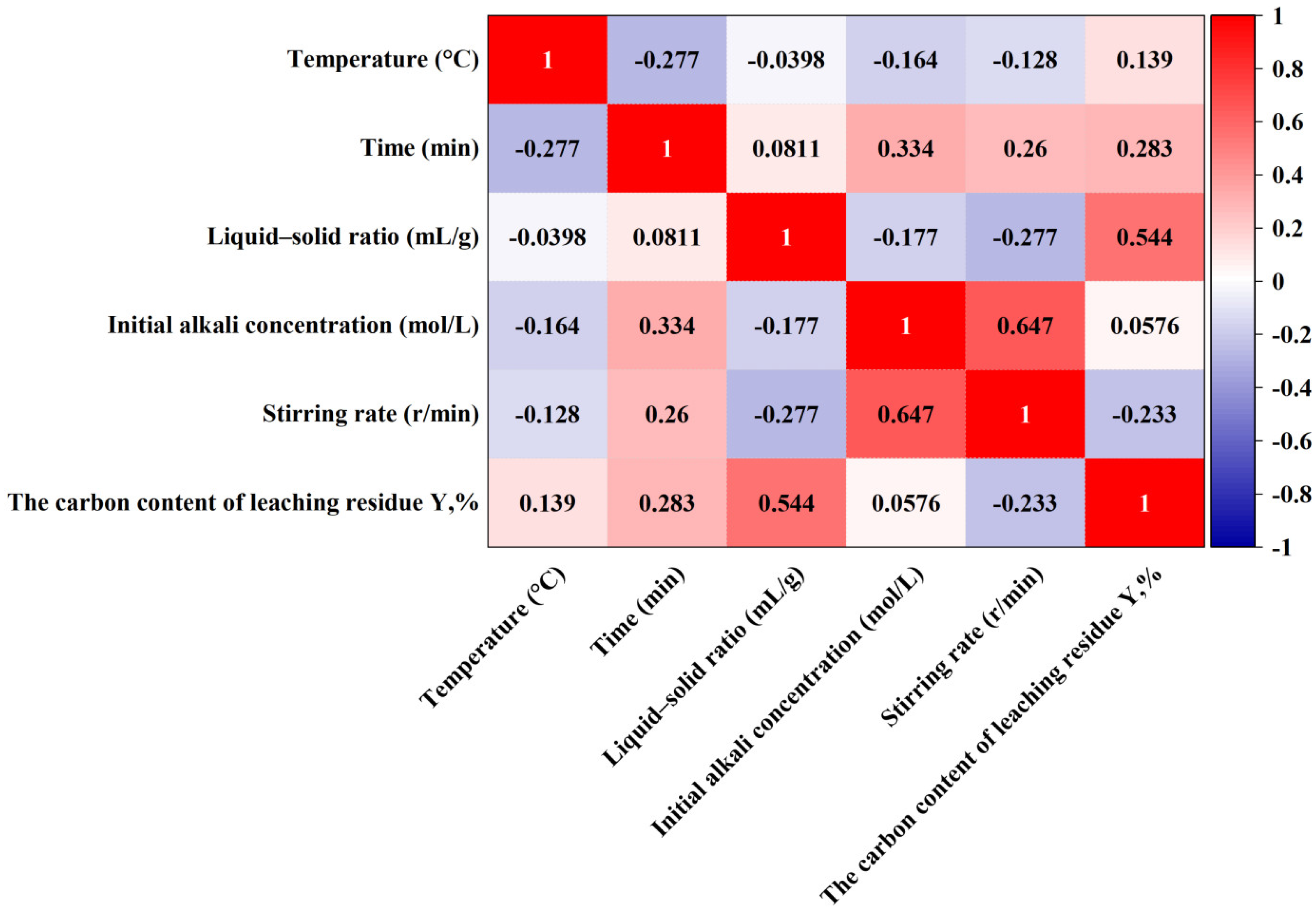
Prior to constructing the ML models, a preliminary investigation of the linear relationships between operational parameters and the carbon content of leaching residues was conducted using Pearson correlation analysis. The variables considered included temperature, leaching time, liquid-to-solid ratio, initial alkali concentration, and stirring rate. The resulting correlation matrix is presented in Figure 1.

As illustrated in Figure 1, the liquid-to-solid ratio exhibits the strongest positive correlation with the carbon content of the leaching residues (r = 0.544), indicating that, from a statistical perspective, increasing the liquid-to-solid ratio favors higher carbon retention in the residue. Leaching time also shows a moderate positive correlation with the target variable (r = 0.283). In contrast, stirring rate demonstrates a negative correlation with residual carbon content (r = −0.233), whereas temperature and initial alkali concentration exhibit relatively weak linear associations with the response. Additionally, certain process parameters are interrelated. For instance, a strong positive correlation is observed between initial alkali concentration and stirring rate (r = 0.647), suggesting that the operational variables are not entirely independent and highlighting potential interaction effects within the input parameter system. The observed correlations further suggest that SCC purification behavior is governed by simultaneous equilibrium and transport-related effects rather than by isolated parameter contributions.

3.2. Comparison of ML Models for Predicting Carbon Content of SCC Leaching Residues

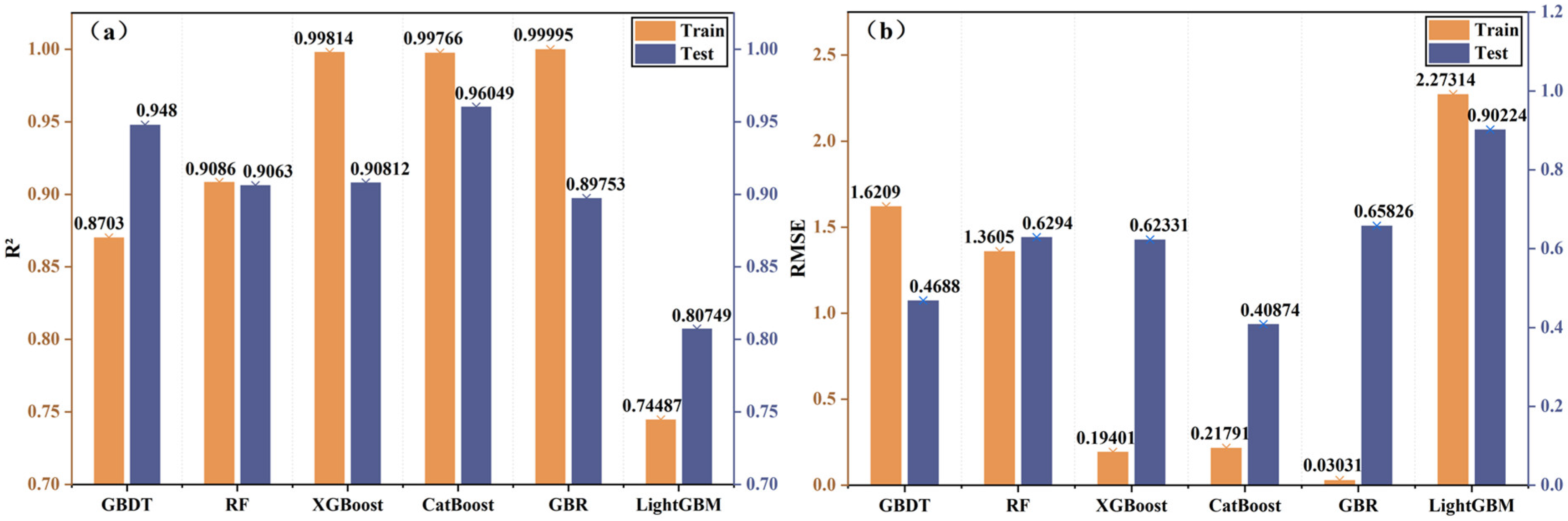
Figure 2 presents a comparison of the predictive performance of six ML models—GBDT, Random Forest (RF), XGBoost, CatBoost, GBR, and LightGBM—for estimating the carbon content of leaching residues from spent cathode carbon (SCC). Model performance was evaluated using the coefficient of determination (R²) and root mean square error (RMSE), with results reported for both the training and testing sets. Higher R² values combined with lower RMSE indicate superior predictive accuracy and generalization capability.

As shown in Figure 2a, the R² values obtained for the training and testing datasets reveal noticeable differences in predictive behavior among the evaluated models. Among all models, CatBoost achieved the highest testing-set R² value (approximately 0.96) while also maintaining a high training-set R² value (approximately 0.98). Both XGBoost and GBR exhibited nearly perfect fitting on the training dataset (R² ≈ 1.00); however, their testing-set R² values decreased to approximately 0.91 and 0.90, respectively. This performance gap suggests that both models experienced a certain degree of overfitting, where the models captured the training data patterns effectively but showed reduced generalization performance on unseen data. Random Forest produced relatively consistent R² values for the training and testing datasets (both around 0.91), reflecting good model stability and balanced predictive behavior. Nevertheless, its overall predictive accuracy remained lower than that of the CatBoost model. In contrast, GBDT exhibited a comparatively lower R² value on the training set (approximately 0.87) but achieved a higher R² value on the testing set (approximately 0.95). This result indicates favorable generalization performance; however, the relatively low training accuracy suggests limited capability in fully capturing the underlying patterns within the training data, implying mild underfitting behavior. Among all evaluated models, LightGBM yielded the lowest R² values for both the training and testing datasets (approximately 0.75 and 0.81, respectively), demonstrating comparatively weak predictive capability and poor adaptability under the current dataset conditions.

Figure 2b presents the comparison of RMSE values for the different models on the training and testing sets. The CatBoost model achieved the lowest RMSE on the testing set (approximately 0.41), with similarly low RMSE on the training set, suggesting a relatively favorable fit under the present data partition, which is consistent with the R² analysis. XGBoost and GBR exhibited extremely low RMSE values on the training set (approximately 0.19 and 0.03, respectively), but the RMSE of their testing set increased noticeably, confirming the presence of overfitting in predicting the carbon content of leaching residues. Random Forest showed comparable RMSE values across training and testing sets, reflecting stable predictions; however, its testing errors were still higher than those of CatBoost. GBDT presented relatively low RMSE on the testing set, but higher RMSE on the training set, suggesting limited capability in capturing complex nonlinear features during training. LightGBM displayed high RMSE values for both training and testing sets, indicating substantial prediction errors and further demonstrating its unsuitability for modeling the current leaching residue dataset.

Among the evaluated algorithms, CatBoost achieved the highest testing-set R² and lowest RMSE. However, in light of the five-fold cross-validation results, which indicate considerable performance variability, this superior performance should be interpreted as ‘relatively better within the current dataset’ rather than as evidence of strong external generalizability.

3.3. Consistency Analysis Between Predicted and Observed Values

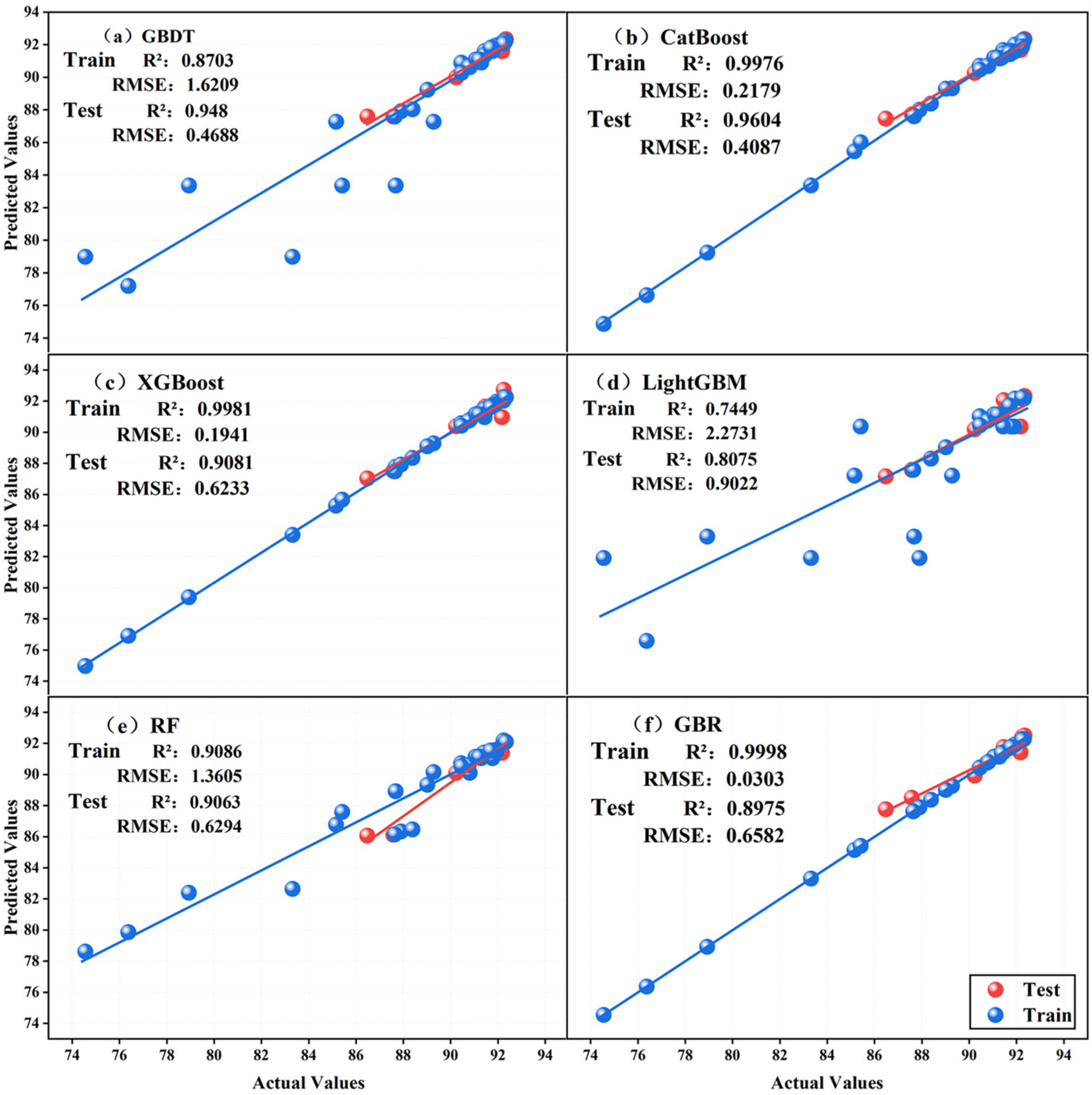
Figure 3 illustrates the comparison between predicted and observed values of the carbon content of leaching residues for GBDT, CatBoost, XGBoost, LightGBM, Random Forest (RF), and GBR models on both the training and testing sets. In the figure, the scatter distribution reflects the prediction accuracy of each model, the fitted line represents the ideal prediction scenario (predicted value = observed value), and the marginal density distributions depict the overall distribution characteristics of the predicted results.

As shown in Figure 3, the predictions of the GBDT model on the training set are relatively dispersed, with some samples clearly deviating from the ideal fitted line, resulting in a relatively low training R² of 0.8703. In contrast, more testing set samples are distributed near the fitted line, with R² increasing to 0.948 and RMSE decreasing to 0.4688.

The CatBoost model showed relatively concentrated prediction points around the ideal line for both the training and testing datasets. The training-set R² and RMSE were 0.9976 and 0.2179, respectively, while the corresponding testing-set values were 0.9604 and 0.4087. Among the evaluated models, CatBoost therefore provided the most favorable combination of testing-set R² and RMSE under the specific 33/9 train–test partition adopted in this study. Nevertheless, the five-fold cross-validation results showed considerable variability in model performance, with a mean R² of 0.2942 ± 0.5905 for CatBoost. This difference between the single-split testing result and the cross-validation result indicates that the apparent predictive performance of CatBoost was sensitive to the composition of the training and validation subsets. Accordingly, the results should be interpreted as evidence of relatively favorable performance within the present dataset and investigated operating domain.

For XGBoost, the training set predictions are almost entirely aligned with the ideal fitted line, yielding a training R² of 0.9981 and RMSE of 0.1941. However, in the testing set, several samples deviate from the fitted line, resulting in a reduced R² of 0.9081 and increased RMSE of 0.6233. This indicates that XGBoost may overfit the training data, exhibiting strong fitting ability on known samples but reduced generalization on unseen data.

LightGBM predictions are more dispersed, with noticeable deviations from the ideal line in both training and testing sets. The training and testing R² values are 0.7449 and 0.8075, respectively, and the RMSE values remain high, suggesting that LightGBM struggles to effectively learn the mapping between variables under the current dataset size and feature conditions.

Random Forest predictions are relatively uniform, with most samples located near the fitted line. The training and testing R² values are 0.9086 and 0.9063, and RMSE values are 1.3605 and 0.6294, indicating good stability, although overall predictive accuracy is slightly lower than that of CatBoost, reflecting some limitations in handling highly nonlinear and strongly coupled variables.

For GBR, the training set predictions are tightly aligned with the ideal line, with a training R² of 0.9998 and RMSE of 0.0303. However, the testing set predictions exhibit greater dispersion, with R² dropping to 0.8975 and RMSE rising to 0.6582, further confirming that GBR, while exhibiting extremely strong fitting capability during training, also suffers from overfitting when applied to predicting the carbon content of leaching residues.

Overall, the comparison of predicted and observed values shows that the six models exhibited substantially different prediction patterns under the present data partition. CatBoost achieved the highest testing-set R² and the lowest testing-set RMSE among the evaluated models. However, the large variability observed in the five-fold cross-validation results indicates that this result is dependent on the composition of the available data and should not be interpreted as evidence that CatBoost possesses universally superior generalization capability. Instead, CatBoost was considered the relatively favorable model for the present dataset and was subsequently used for SHAP-based interpretation. This selection was made to investigate the model-attributed relationships learned from the available data, rather than to establish that CatBoost is universally superior to the other algorithms.

3.4. SHAP-based Feature Contribution Analysis Using Catboost Model

To further elucidate the influence of operational parameters on the carbon content of leaching residues, SHapley Additive exPlanations (SHAP) was applied to interpret the CatBoost model [25,28]. While SHAP analysis provides a quantitative decomposition of model predictions into feature contributions, it is important to note that SHAP reflects the behavior of the trained model rather than establishing direct causality [26]. Therefore, the SHAP results are interpreted in conjunction with established physicochemical principles of leaching processes to provide mechanistically meaningful insights. Furthermore, the input variables are not statistically independent; for example, initial alkali concentration and stirring rate exhibit a Pearson correlation of 0.647 (Figure 1). Such multicollinearity can affect SHAP attribution, potentially overestimating or underestimating the importance of correlated features. Therefore, our interpretation emphasizes the overall ranking and qualitative directional effects rather than the precise SHAP value magnitudes.

3.4.1. Global Feature Importance and Process Significance

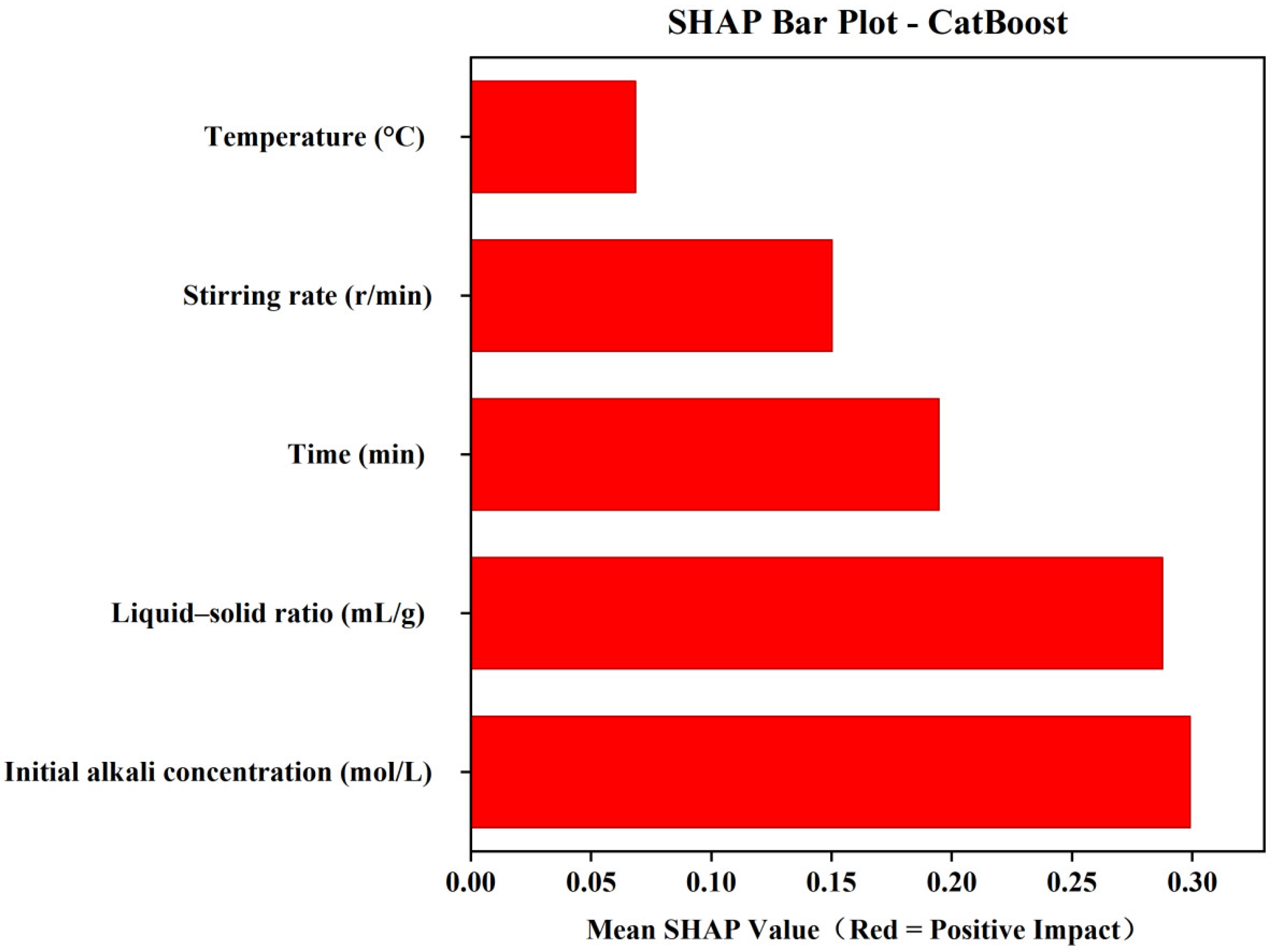
Figure 4 presents the mean absolute SHAP values, indicating the relative importance of input variables. The mean absolute SHAP analysis yielded the following model-attributed importance ranking: initial alkali concentration > liquid-to-solid ratio > leaching time > stirring rate > temperature. The ranking describes the relative contributions of the available input variables to the model predictions. This hierarchy is consistent with the fundamental controlling mechanisms of heterogeneous leaching systems [17,37,38,39]. Initial NaOH concentration exhibited the largest model-attributed contribution among the input variables included in the model. Higher NaOH concentration was associated with a larger positive or negative SHAP contribution to the model-predicted residual carbon content, depending on the local sample conditions. This association is consistent with the expected influence of reagent concentration on alkaline leaching chemistry, but the present data do not establish a causal relationship.

The liquid-to-solid ratio represents a key parameter controlling mass transfer conditions. Increasing this ratio improves reagent accessibility and reduces diffusion limitations at the solid–liquid interface [39]. From a transport perspective, a higher liquid volume enhances the concentration gradient between the bulk solution and the particle surface, thereby promoting the removal of soluble species [40]. These considerations provide a possible physicochemical interpretation of the relatively large SHAP contribution observed for this variable, but the present dataset does not directly quantify diffusion resistance or mass-transfer coefficients.

In contrast, leaching time exhibits a moderate contribution, suggesting that the system may approach a quasi-equilibrium state within the investigated time range. Once readily soluble components are removed, further extension of leaching time provides diminishing returns, consistent with typical shrinking-core or diffusion-limited leaching behavior reported in similar systems [41,42,43].

The relatively small SHAP contributions of stirring rate and temperature indicate that these variables had weaker model-attributed associations with the predicted carbon content than initial alkali concentration and liquid-to-solid ratio within the investigated operating ranges. However, the present data do not allow direct determination of whether external mass transfer, internal diffusion, reaction kinetics, or chemical equilibrium represents the dominant rate-controlling factor.

The relatively weak SHAP contribution of temperature indicates that temperature exhibited a comparatively weaker model-attributed contribution to the predicted response within the investigated operating range. This observation should not be interpreted as evidence that temperature is kinetically unimportant, because the present dataset does not contain sufficient kinetic information to distinguish among reaction-control, diffusion-control, and other possible limiting regimes.

3.4.2. Directional Effects and Interaction Mechanisms

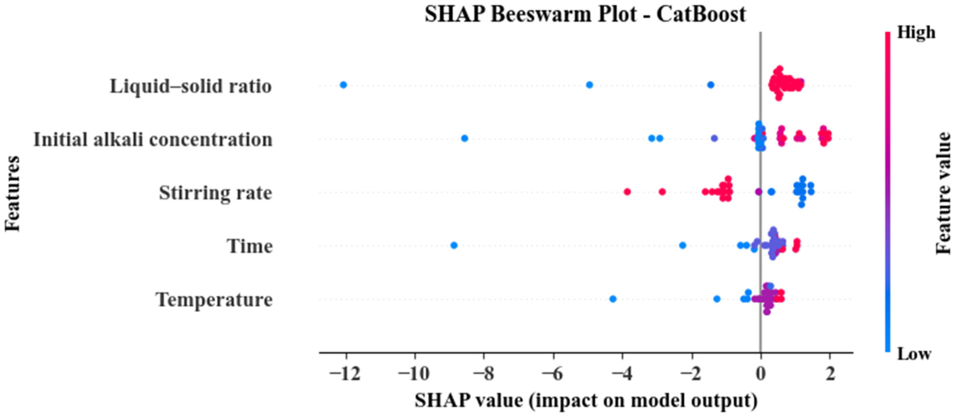
The SHAP beeswarm plot in Figure 5 provides further insight into the directionality of parameter effects. For the dominant variables, higher feature values tend to exhibit consistent directional contributions, which can be interpreted through process mechanisms.

For the liquid-to-solid ratio, higher values generally show positive SHAP contributions to residual carbon content. This can be attributed to improved removal of soluble impurities while leaving the carbon matrix relatively intact. Enhanced liquid availability reduces localized saturation effects and facilitates the transport of dissolved species away from the particle surface, thereby increasing the apparent carbon fraction in the residue.

Similarly, initial alkali concentration shows predominantly positive contributions at higher values. From a chemical standpoint, the positive SHAP contributions observed at higher alkali concentrations are consistent with the possibility that increased alkali availability promotes the dissolution of alkali-reactive impurity phases. However, excessive concentration may also alter solution chemistry and affect selectivity, indicating that its effect is not purely linear but coupled with other variables [44].

The stirring rate exhibits mixed SHAP contributions, reflecting its secondary role in the process. At low stirring rates, insufficient mixing may lead to local concentration gradients and reduced leaching efficiency. At higher stirring rates, external mass transfer limitations are minimized, but further increases provide limited benefit once the system transitions to internal diffusion control. This may help explain the bidirectional SHAP distribution learned by the trained model.

For leaching time and temperature, the SHAP values are relatively clustered around zero, indicating weaker and condition-dependent effects. This suggests that, within the studied experimental window, the system may already operate near effective temperature and time conditions, beyond which additional increases do not significantly enhance impurity removal or carbon preservation.

3.4.3. Implications for Process Understanding and Model Interpretation

Finally, we reiterate that the mechanistic interpretations offered here are hypotheses derived from the model’ s learned associations and are supported by established leaching theory. They are not directly proven by the ML model itself. Independent experimental studies, such as time-resolved concentration measurements or particle characterization, are required to confirm the proposed reaction–transport mechanisms. Our contribution lies in using SHAP to prioritize which variables and interactions deserve closer experimental scrutiny.

The combined SHAP analysis and cautious comparison with established leaching theory suggest that SCC leaching is governed by a coupled interplay of chemical reaction equilibrium and mass transfer processes, rather than being dominated by a single kinetic factor. The dominant role of liquid-to-solid ratio and alkali concentration highlights the importance of reagent availability and transport conditions, while the relatively minor role of temperature and stirring rate indicates limited sensitivity to external kinetic enhancement within the investigated range.

It is important to emphasize that SHAP analysis provides model-based inference rather than direct mechanistic proof. However, when interpreted alongside established leaching theory, the results offer a consistent and physically meaningful explanation of parameter effects. This integration of data-driven interpretation with process-level understanding enhances the reliability of the conclusions and provides a more robust basis for process optimization [45,46,47].

The present study did not include concentration–time profiles, particle-size evolution, kinetic model fitting, effective diffusivity measurements, or mass-transfer calculations. Therefore, the observed feature contributions cannot independently verify reaction-control, diffusion-control, external mass-transfer limitation, or shrinking-core behavior. These mechanisms are discussed only as plausible hypotheses that may explain the observed statistical associations and require independent experimental verification.

3.5. Implications for Experimental Prioritization and Process Screening

The findings of this study provide important engineering insights into the purification and resource utilization of SCC. As SCC is a hazardous by-product generated during aluminum electrolysis, improving the efficiency and controllability of the leaching process is essential for reducing environmental risks and supporting sustainable recycling strategies [1,2,3,4,5]. Within the available dataset, initial alkali concentration and liquid-to-solid ratio showed relatively large model-attributed contributions to the predicted carbon content of the caustic-leaching residue. These variables may therefore represent priority factors for subsequent experimental investigation, particularly when the objective is to understand variations in the carbon content of the residue.

From a sustainability perspective, more targeted parameter optimization may contribute to reducing unnecessary chemical consumption, water usage, and energy demand during SCC treatment. Such improvements are important for enhancing the environmental and economic performance of recycling processes, particularly in industrial systems where large-scale experimental optimization is often time-consuming and resource intensive. The integration of interpretable ML with physicochemical understanding therefore provides a practical approach for accelerating process evaluation and identifying key operational variables under limited experimental conditions [20,48,49].

More broadly, this study demonstrates the potential of interpretable ML as a complementary tool for supporting data-assisted decision-making in hydrometallurgical and recycling systems. Beyond predictive capability, the proposed framework enables quantitative interpretation of parameter effects and provides process-relevant insights into coupled reaction and transport mechanisms. The methodology may therefore be extended to other complex leaching and resource recovery systems, contributing to the development of more intelligent, efficient, and sustainable metallurgical process optimization strategies.

The present study should be distinguished from the original experimental work used to construct the dataset. The original study focused on experimentally optimizing the purification process using single factor experiments and response surface methodology. In contrast, the present work does not introduce new experimental conditions or claim to replace the original experimental optimization. Instead, it provides a complementary data-driven analysis of the published observations by comparing multiple nonlinear ML models and interpreting their model-attributed feature contributions.

4. Conclusions

The evaluated ML models captured nonlinear relationships between the operating parameters of the NaOH-based caustic-leaching stage and the carbon content of the resulting caustic-leaching residue. Among the evaluated models, CatBoost yielded the most favorable performance under the specific train–test partition used in this study and also produced the highest mean R² and lowest mean RMSE in the five-fold cross-validation comparison. Even though the results from the five-fold cross-validation showed some instability, they can still serve as an important reference for later interpretability analysis.

SHAP-based interpretation further revealed that the influence of process parameters followed the order: initial alkali concentration > liquid-to-solid ratio > leaching time > stirring rate > temperature. SHAP analysis, interpreted cautiously, consistently identified initial alkali concentration and liquid-to-solid ratio as the most influential variables associated with residual carbon content and aligns with the physicochemical understanding that chemical driving force and mass transfer are key controlling factors in SCC leaching.

Although the ML models evaluated in this study provided predictions of the carbon content, several limitations should be acknowledged. The relatively small dataset, consisting of 42 experimental samples with only 9 samples used for testing, may limit the broader generalization capability of the developed models under substantially different operating conditions. Consequently, the model predictions primarily reflect interpolation within the investigated parameter ranges and should be interpreted cautiously when extrapolated beyond the available experimental space. Although five-fold cross-validation was conducted to evaluate model robustness, the limited dataset size may still introduce uncertainty regarding broader model generalization. In addition, the present study focused mainly on predicting the residual carbon content of the leaching residues, whereas direct evaluation of impurity removal efficiency and purification selectivity requires further investigation.

Future work should focus on expanding the experimental dataset, incorporating independent external validation datasets, and integrating physics-informed or hybrid ML approaches to further improve prediction reliability and mechanistic interpretability. Overall, this study demonstrates that interpretable ML provides a promising and practical approach for linking process variables with leaching performance, while supporting data-assisted optimization and sustainable process development in hydrometallurgical recycling systems.