
Article

Detection of the Structure and Seepage Pathways of a Tailings Pond Using Electrical Resistivity Tomography at the Husab Mine, Namibia

1
College of Environment and Civil Engineering, Chengdu University of Technology, 1#, Dongsanlu, Erxianqiao, Chengdu 610059, China
2
Uranium Resources Co., Ltd., China General Nuclear Power Corporation, 18/F, Tower A, Guangya Dongfang, No.100, West 3rd Ring North Road, Haidian District, Beijing 100048, China
*
Author to whom correspondence should be addressed.
Minerals 2026, 16(7), 723; https://doi.org/10.3390/min16070723
Submission received: 12 May 2026 / Revised: 1 July 2026 / Accepted: 6 July 2026 / Published: 10 July 2026

Abstract

The phreatic surface and seepage field are key factors causing instability in tailings storage facilities (TSFs). In this study, electrical resistivity tomography (ERT) was used to determine the internal structure and phreatic surface of the TSF of Husab Mine. The seepage pathways at the southeast and northwest corners of the TSF were identified and the seepage mechanisms were analyzed. In order to discharge the slurry, outlets equipped with valves were installed on the tailings embankment. During the deposition process, time-lapse electrical resistivity tomography (TL-ERT) was conducted to monitor the infiltration of water around the W13 outlet. The results show that the tailings sediments were divided into three layers based on resistivity values. The top layer consisted of shallow, unsaturated tailings material, while the middle layer comprised saturated tailings material. The thickness of the saturated zone gradually increased from the dam toward the decant pool. The bottom layer consisted of the geomembrane liner and natural sediments. Two seepage locations, named the Lebusa corner and Alister corner, were located at the southeast and northwest corners of the TSF, respectively. Seepage occurred because clarified water originating from the decant pool migrated through the saturated zone of the tailings pond, along the base of the tailings embankment. Upon encountering the starter dam, the water was impeded and subsequently emerged as seepage at the junction between the starter dam and the tailings embankment. TL-ERT monitoring shows that the extent of increased moisture was approximately 60 m horizontally and roughly 10 m vertically due to deposition at the W13 outlet.

1. Introduction

Tailings storage facilities (TSFs) constitute engineered systems designed to contain the residual by-products (i.e., tailings) of metal ore extraction and manage associated process water. Globally, approximately 13 billion tonnes of mine tailings are deposited in TSFs annually [1]. The failure rate of TSFs over the past 100 years has been estimated at 1.2%, based on a database inventory of 18,401 mine sites worldwide [2]. TSF failures and associated disasters have historically had disastrous environmental, social, and economic impacts. Since 1915, 257 TSF failures have occurred, with subsequent release of approximately 250 million m3 of tailings, resulting in an estimated 2650 deaths and impacting 31.7 million people [3].
A range of mechanisms (i.e., earthquake, slope instability, seepage, weak foundation, overtopping, and mine subsidence) result in the failure of TSFs. Seepage and internal erosion comprise the third most frequent cause, responsible for 9% of tailings dam failures [3,4]. Seepage and internal erosion initiate in the form of concentrated leak erosion, contact erosion, internal migration, and backward erosion piping under material susceptibility, critical stress, and hydraulic conditions [5].
The phreatic surface and seepage field are key factors in TSF instability. For example, high water levels and piezometric surfaces were critical factors that triggered the Stava disaster in Italy (1985) and the Brumadinho dam collapse in Brazil (2019) [3,6]. The phreatic surface within the TSF remains low to ensure the stability of the tailings dam when the tailings medium exhibits high permeability and the drainage system functions effectively. Monitoring of seepage flow and pore pressure with piezometers is an important component of TSF management. The spatial and temporal variations of seepage data can provide precursory information on seepage and internal erosion [7,8]. Piezometers are limited by high costs and their invasive nature when applied to large-scale measurements.
Due to their non-invasive measurement and ability to acquire abundant data (i.e., 2D or 3D), geophysical methods are becoming effective complementary tools for seepage detection in TSFs. Electrical resistivity tomography (ERT) is a geophysical technique employed to image the subsurface distribution of electrical resistivity [9]. ERT is primarily performed for groundwater and mineral exploration based on resistivity contrasts [10]. Integrated geophysical techniques, including ERT, magnetic, ground penetrating radar (GPR), and multi-channel analysis of surface waves (MASW), are used for the exploration of bauxite, chromite, and coal deposits [11,12,13,14]. Water seepage in the underground coal mine barrier can also be mapped with ERT and self-potential methods [15,16,17].
As the seepage water in TSFs is electrically conductive, ERT has been used to evaluate acid mine drainage and dam instability [18,19], image the internal structure [20,21,22], and conduct physical–chemical characterization [23,24]. Furthermore, permanent arrays are installed within TSFs to conduct time-lapse electrical resistivity tomography (TL-ERT) monitoring [25]. TL-ERT has been employed to track leachate infiltration in heap leaching pads [26], monitor the stability of TSFs [27], and characterize subsurface flow [28].
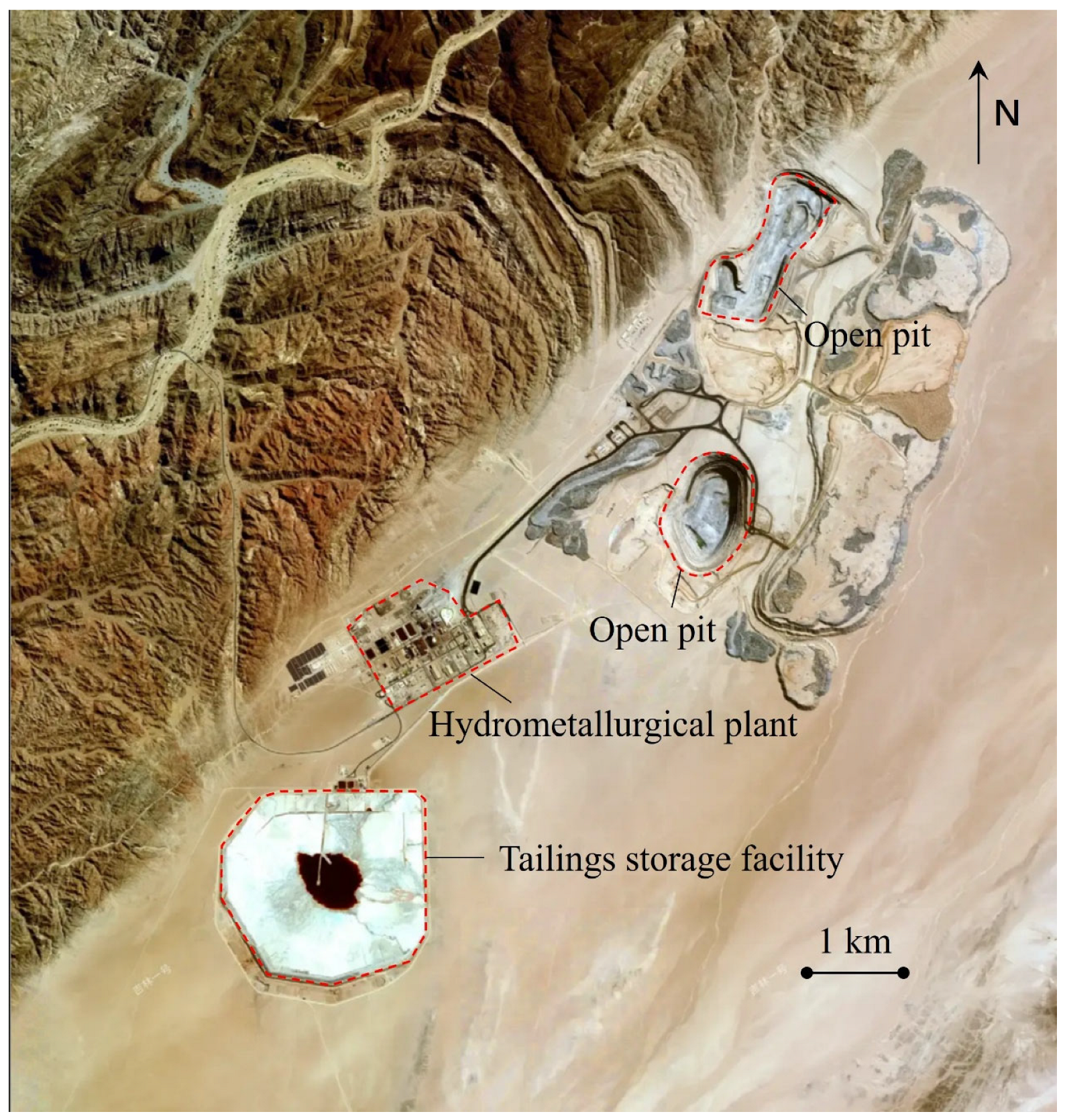
The Husab Mine is an open-pit uranium mine located in the Erongo Region of west–central Namibia (Figure 1). It stands as one of the largest uranium mines globally. The TSF of Husab Mine, commissioned in December 2016, is located southwest of the open-pit operation and the hydrometallurgical plant (Figure 2). Designed with a storage capacity of approximately 182 million m3 and a 20-year service life, the TSF of Husab Mine is fully capable of accommodating the estimated 301 million tonnes of tailings generated by the hydrometallurgical plant. The TSF of Husab Mine was commissioned in December 2016; after five years of operation, localized seepage was observed on the tailings dam. In this study, ERT was used to detect the internal structure and phreatic surface of the TSF of Husab Mine. The seepage pathways were identified and the seepage mechanisms were subsequently analyzed. In addition, TL-ERT was conducted to monitor the infiltration of water during the deposition process.

2. Site Description

2.1. Physical Geography of the Region

The Husab Mine is located within the Namib Naukluft National Park in the Erongo Region of western Namibia. It is situated approximately 65 km from the coastal city of Swakopmund and 110 km from Walvis Bay, which is the largest deep-water port in southwest Africa (Figure 1).
The Husab Mine lies on the northern side of a rough triangle bounded by two major ephemeral rivers. The Khan and Swakop rivers are located in the northern and southern parts of the region, respectively. An open plain, sloping gently toward the Swakop river, occupies the area between the two rivers. The area is interspersed with limestone ridges and granite outcrops. The valleys of the Swakop and Khan rivers are deeply incised, lying approximately 200 m below the elevation of the watershed. The landscape to the southeast is dominated by Husab Mountain, the eponym of the mine. Several shallow, sandy watercourses traverse the gravel plains from northeast to southwest. These watercourses supply the extensive Welwitschia mirabilis field located south of the Husab Mine site.
The Husab Mine is situated within a hyper-arid region, with a long-term annual average rainfall of less than 50 mm [29]. Spatial and temporal variability in rainfall is high. Based on monitoring data, the annual rainfall in the mining area is typically less than 5 mm. The potential annual evaporation is between 1960 mm and 2100 mm. In this area, summers are moderately hot with an average maximum temperature of 30 °C; in comparison, winters are cool, with an average minimum temperature of 10~12 °C.

2.2. Tailings Storage Facility of the Husab Mine

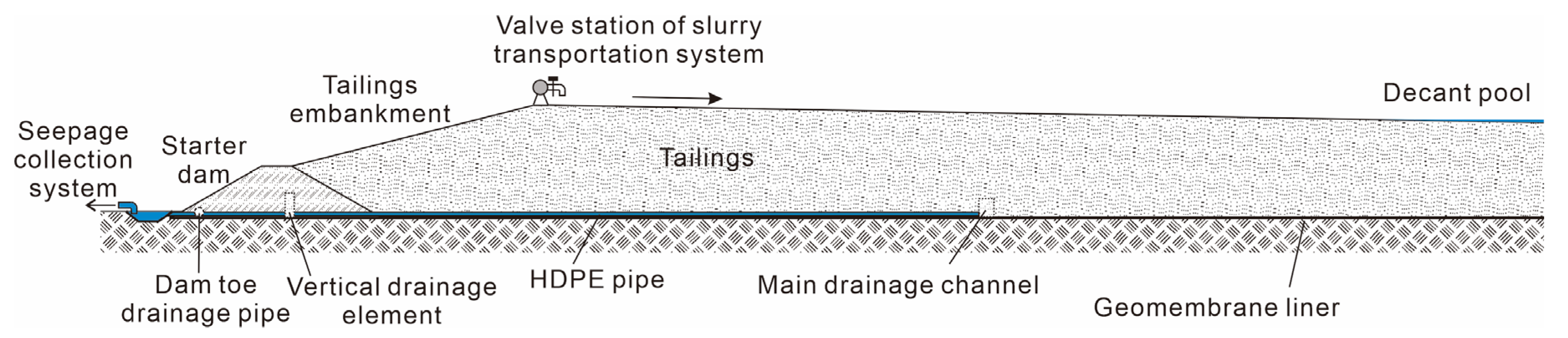
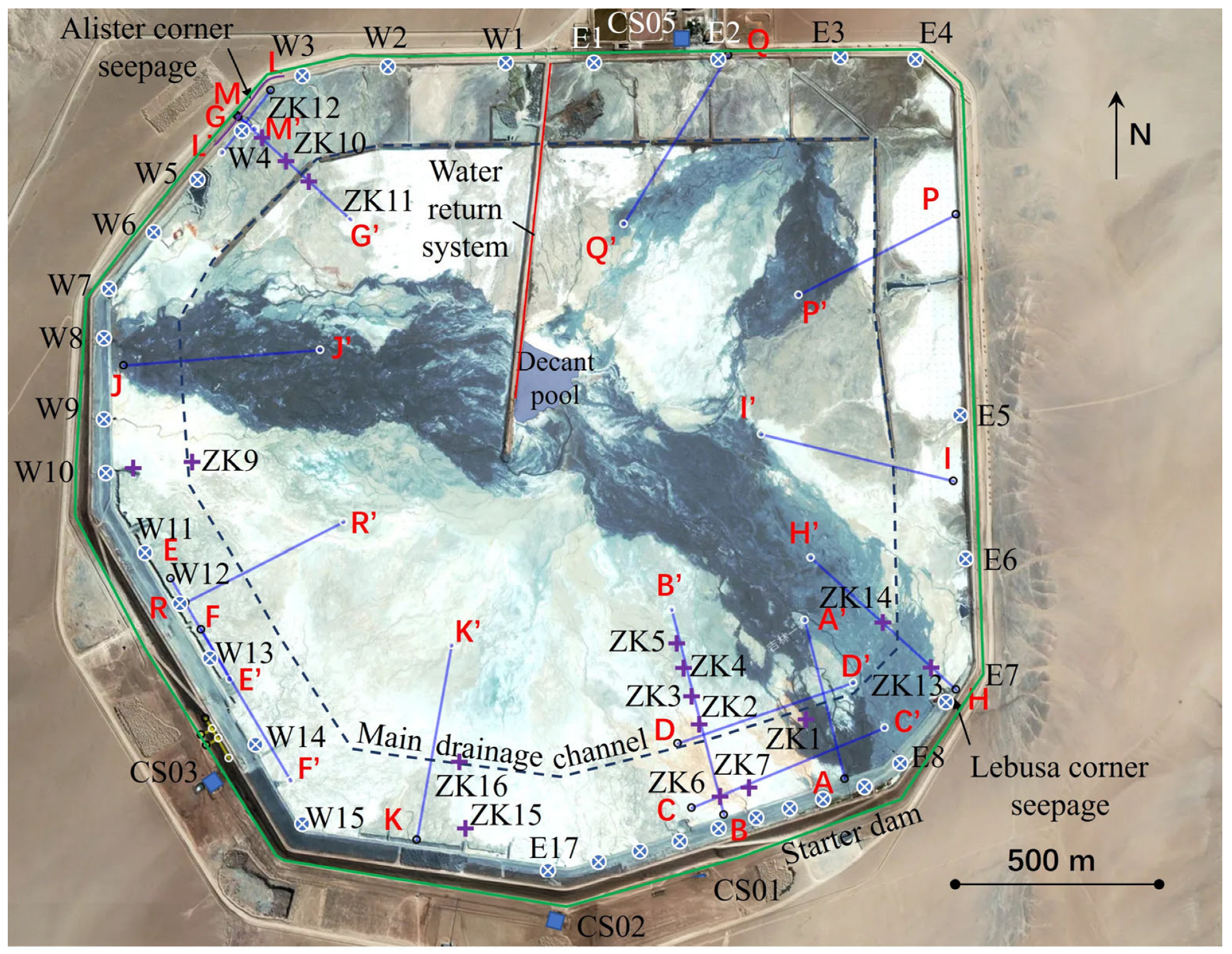
The tailings storage facility of the Husab Mine is a typical wet tailings storage facility situated on flat ground (Figure 2). The tailings storage facility spans approximately 2.2 km from east to west and 2.0 km from north to south, with a total area of roughly 4.2 km2. The tailings storage facility primarily consists of a bottom geomembrane liner, a starter dam, a tailings embankment, a slurry transportation system, a seepage drainage system, a seepage water collection system, and a water return system (Figure 3 and Figure 4).
The geomembrane liner, comprising low-density polyethylene (LLDPE) geomembranes of 1.0 mm thickness, was installed over the tailings pond area and the base of the starter dam. The starter dam was an earth–rockfill dam constructed from calcified soil and block stones excavated from the tailings pond area. The dam was built by means of layered compaction. The designed crest elevation of the starter dam is 483.0 m. The dam height varies according to the original ground elevation. The maximum dam height on the southern side of the tailings pond is 17 m, whereas the minimum height is 3 m at locations where the original ground elevation exceeds 480 m. Both the upstream and downstream slopes of the starter dam feature a gradient ratio of 1:1.75, and the dam crest is 10 m wide. After the starter dam reached full capacity, construction continued using the upstream method with tailings sediments. The designed slope ratio of the tailings embankment is 1:4, with a maximum raising rate of 3.25 m per year.
The slurry transportation system consists of two ore-drawing pipelines (eastern and western), both of which are constructed from rubber-lined steel pipes with a diameter of 500 mm. Ore-drawing ports were installed every 200 m along the slurry transportation pipelines. The valve stations for the eastern and western pipelines are sequentially numbered starting from E1 and W1, respectively, progressing southward from the location near the hydrometallurgical plant. The eastern and western parts of the tailings pond contain 17 and 15 valve stations, respectively (Figure 3). To ensure the safe operation of the TSF, only two opposing valve stations (one on the east side and the other on the west side) were opened during the deposition process. Each valve station remained open for deposition for approximately 8 h.
The seepage drainage system was installed above the geomembrane liner at the bottom of the pond. The seepage drainage system consists of a main drainage channel, vertical drainage elements, and dam toe drainage pipes (Figure 4). The main drainage channel was arranged parallel to the starter dam in a ring-shaped plan layout, located approximately 200 m inland from the upstream dam toe of the starter dam. It was constructed on a 3 m high, 5 m wide embankment and comprises drainage trenches and drainage pipes. The drainage trench was backfilled with the non-calcareous material and wrapped with an external geotextile filter layer. Vertical drainage elements with a width of 600 mm were embedded within the starter dam. Their heights varied according to the elevation of the starter dam. Dam toe drainage pipes were installed along the outer dam toe lines of the southern and southwestern sections of the starter dam.
The seepage collection system consists of four ponds (i.e., CS01, CS02, CS03, and CS05, as shown in Figure 3), with a geomembrane liner at the base. The seepage water is ultimately collected in the pond CS03 on the southern side and recycled to the hydrometallurgical plant (Figure 4). The water return system is used to recover clarified water within the central decant pool. Several recycled water wells were constructed to improve the drainage capacity. Because the hydrometallurgical plant employs an acid leaching process, the chemical characteristics of the seepage water in the tailings pond were defined as follows: pH 1.8~3.6, TDS 33,486~58,715 mg/L, and EC 20.44~29.00 mS/cm.

3. Data Acquisition and Processing

3.1. Data Acquisition and Processing of ERT

ERT is performed by injecting electrical current into the ground through one pair of electrodes (current electrodes) and measuring the resulting electrical potential differences using another pair of electrodes (potential electrodes). In field surveys, ERT measurements are conducted using a multi-electrode array composed of tens to hundreds of electrodes. The prospecting depth increases with the separation of the current and potential electrodes.
Figure 3 illustrates the layout of ERT profiles. A total of 16 profiles were conducted to investigate the structure and seepage pathways of the tailings pond. Table 1 presents the detailed information for all profiles. The Wenner array and Schlumberger array were used due to their good signal strength and vertical resolution [9]. The electrode spacing ranged between 1 m and 5 m. The maximum spacing factor was 25 for most profiles, with a few (i.e., J−J’ and K−K’ profiles) reaching 30. A total of 56,523 pieces of apparent resistivity data were collected. The elevation data of the ground surface along ERT profiles were measured with real-time kinematic (RTK) positioning.
The ERT surveys were conducted using a DZD−8A Multi−function Full Wave DC Electron Meter (CGE Chongqing Geological Equipment Co., Ltd., Chongqing, China). Other equipment included copper electrodes, DC batteries, cables with a 5 m electrode spacing, cascaded converters connecting cables, and a boost power supply. Before measurement, the ground resistance was tested to ensure good contact between the electrodes and the ground. In general, the ground resistance should be kept below 1 kΩ. For electrodes with a ground resistance exceeding 1 kΩ, the surrounding sand must be moistened with water. If the ground resistance still fails to meet the required threshold, the measurement data associated with these electrodes are excluded during data processing. During the measurement process, the power-on and power-off durations were 0.5 S and 0.1 S, respectively. The minimum current was set to 10 mA. The gradient threshold of potential was set to 100 mV/s. For each profile, the measurement was completed in approximately 20–30 min.
The apparent resistivity data with measurement errors greater than 5% were removed prior to inversion. More than 93% of the data were retained on ERT profiles. The apparent resistivity data were inverted using Res2dinv software (version 3.54) based on the least-squares method [30]. The initial model is iteratively revised to minimize the discrepancy between the model response and the observed data values. The smoothness-constrained Marquardt–Levenberg inversion formulation is given by the following:
J T J + λ F Δ q = J T g
where J is the Jacobian matrix of partial derivatives; F is the matrix including smoothing matrices in horizontal and vertical directions [31]; the factor λ is the Marquardt or damping factor; Δ q is the change vector of model parameters; and g is the discrepancy vector between the observed data and the model response. After calculating the parameter change vector Δ q , a new model is obtained by the following:
q k + 1 = q k + Δ q k
where q k and q k + 1 are the model parameters obtained after k and k + 1 iterations, respectively.
The topography data were incorporated into the inversion model. Due to the significant variation in resistivity, the cell width was set to half the unit electrode spacing to achieve more accurate inversion results. In general, the resistivity distribution and root mean square (RMS) stabilized after three or four inversion iterations.
In this study, ERT was primarily used for static measurements of structure and seepage. The evaluation of water infiltration depth and extent during the deposition process is also important for understanding vertical water recharge in the TSF. TL-ERT was conducted to monitor the infiltration of water around the W13 outlet (Figure 3). During TL-ERT measurement, cables were placed along the boundary between the inner side of the tailings embankment and the loose tailings. For data inversion of TL-ERT measurement, the inversion model from the initial data set was used as a reference model in the inversion of subsequent data sets. Data from time-lapse surveys conducted at different time points were inverted simultaneously [32]. The robust smoothness constraint was used to minimize the absolute changes in the model resistivity values [33]. After five iterations of inversion, the RMS value dropped to 2.47 and stabilized.

3.2. Borehole Layout and Parameter Measurement

During the investigation, a total of 16 boreholes were drilled within the TSF (Figure 3). The samples obtained from these boreholes were used to determine the dry density and water content. Drilling was terminated upon reaching the saturated zone because sampling could not be conducted under these conditions. The maximum depth of boreholes was also limited to 9 m to avoid damaging the geomembrane liner at the base. Tailings samples were collected with 100 cm3 cutting rings. The dry density and gravimetric water content of samples were determined using the standard oven-drying method [34]. The volumetric water content (VWC) of samples is equal to the dry density multiplied by the gravimetric water content.

4. Results and Discussion

4.1. Survey Results in the Southeast Area

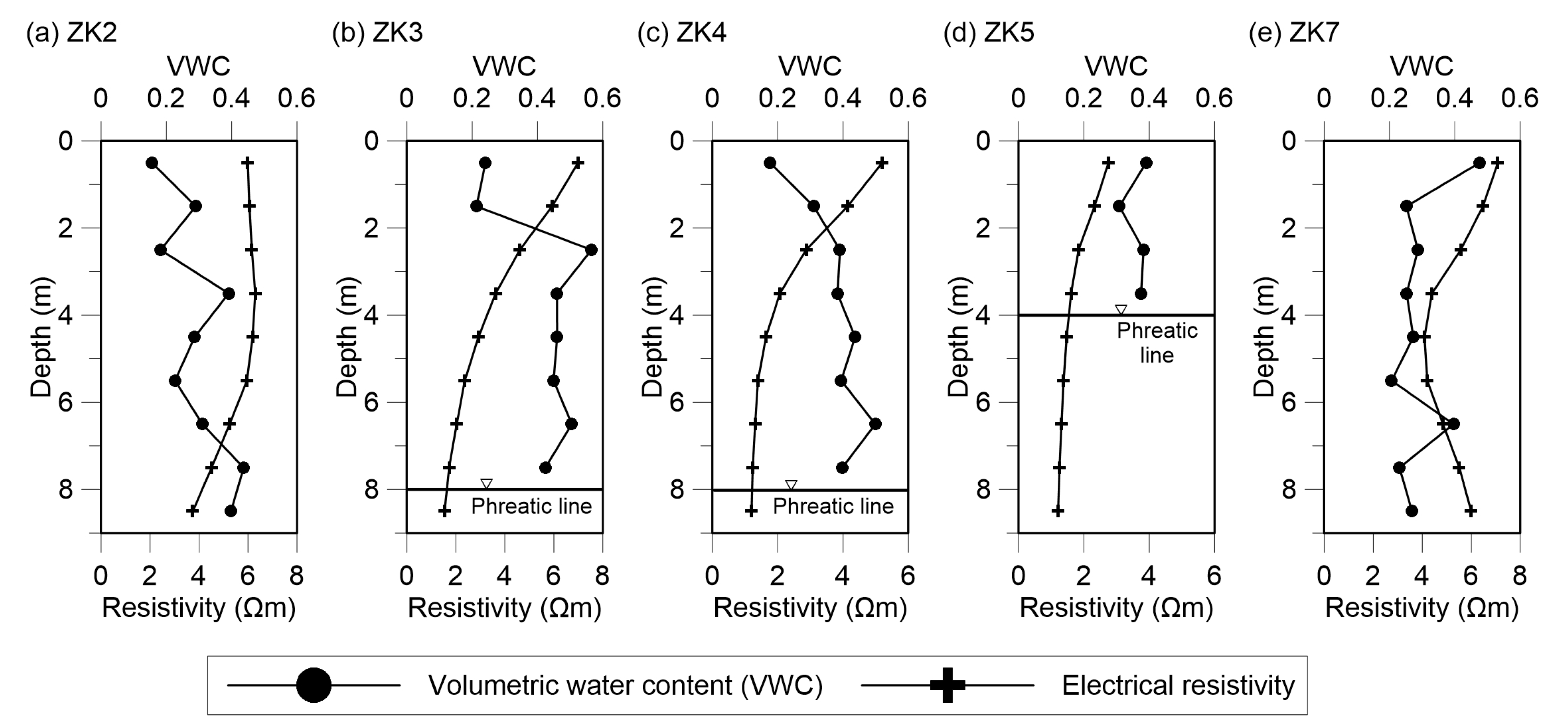
Figure 5 presents the results of the ERT survey in the southeast area of the TSF. Figure 6 highlights variations in the resistivity and volumetric water content at boreholes. Boreholes ZK2, ZK3, ZK4, and ZK5 were located on the B−B’ profile, whereas borehole ZK7 was situated on the C−C’ profile.
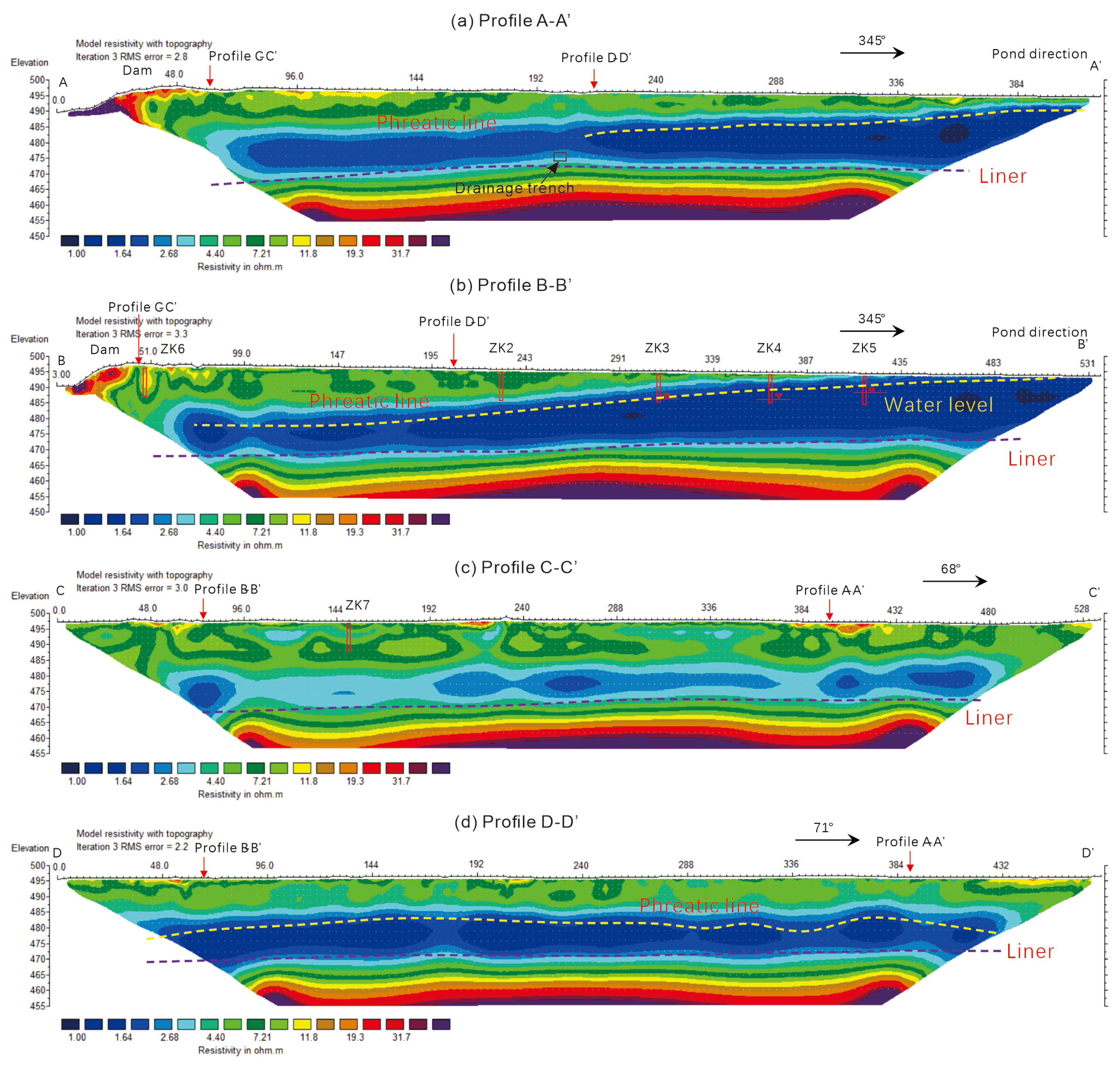
The A−A’ and B−B’ profiles extended from the tailings dam toward the decant pool (Figure 5a,b). As shown in the figures, the subsurface could be divided into three layers based on resistivity values. The first layer consisted of shallow unsaturated tailings material with resistivity generally ranging between 1.6 Ωm and 12 Ωm (i.e., blue, green, and yellow areas). In this zone, tailings form a porous medium composed of solid, liquid, and gas phases, where current was conducted only through water in the liquid phase, resulting in higher resistivity. Based on the borehole sampling test results (Figure 6), the volumetric water content of the tailings exhibited an increasing trend with depth. The volumetric water content of the tailings near the surface was approximately 0.2, increasing to more than 0.4 within a depth of several meters.
The second layer comprised saturated tailings material with resistivity values ranging between 0.8 Ωm and 1.6 Ωm (i.e., dark blue area), forming a saturated porous medium of solid and liquid phases. The conductivity of slurry water exceeded 20 mS/cm, indicating electrical conductivity. In the middle of the A−A’ profile, the saturated layer of low resistivity appeared discontinuous, which was attributed to the drainage trench of the main drainage body. The thickness of the saturated zone gradually increased from the dam toward the decant pool. The depth of the phreatic surface was more than 17 m near the tailings dam. Borehole ZK6 exhibited a phreatic surface depth exceeding 9 m (Figure 5b). The phreatic surface shoaled toward the decant pool, ultimately intersecting the ground surface at the pool’s edge. Sampling at a depth of 8 m in boreholes ZK3 and ZK4 resulted in water emerging from the samples, whereas borehole ZK5 was found to have a water table depth of approximately 4 m (Figure 6). Borehole sampling tests indicated that the volumetric water contents at the phreatic surface were between 0.4 and 0.5, with an electrical resistivity of less than 1.6 Ωm.
The third layer consisted of the underlying natural sediments and a geomembrane liner made of low-density polyethylene (LLDPE) with resistivity greater than 2 Ωm. LLDPE is an insulating material with resistivity of 100 to 1000 Ωm. Due to the smoothing constraints during the inversion process, an artifact transition zone appeared between the low-resistivity and deep high-resistivity regions in the ERT results. The original terrain elevation for the A−A’ profile ranged from 472.0 to 474.6 m, whereas for the B−B’ profile, it varied from 469.8 to 473.7 m. Resistivity distribution indicates that the geomembrane liner at the base of the tailings dam was generally intact.
Figure 5c presents the results of the ERT survey for the C−C’ profile, which was close to and parallel to the dam. The results show that the tailings material was predominantly unsaturated, with only isolated areas of high moisture content in deeper sections. High resistivity values in deeper sections indicated the elevation of the geomembrane liner at approximately 470 m.
Figure 5d presents the findings of the ERT survey for the D−D’ profile. The profile was located 150 m north of the C−C’ profile and parallel to the dam. The distribution of resistivity was divided into three stable layers from top to bottom: the unsaturated zone, the saturated zone, and the geomembrane liner. The distribution of the saturated zone was relatively consistent, with the phreatic surface elevation ranging from 480 m to 485 m.

4.2. Survey Results in the East and Northeast Area

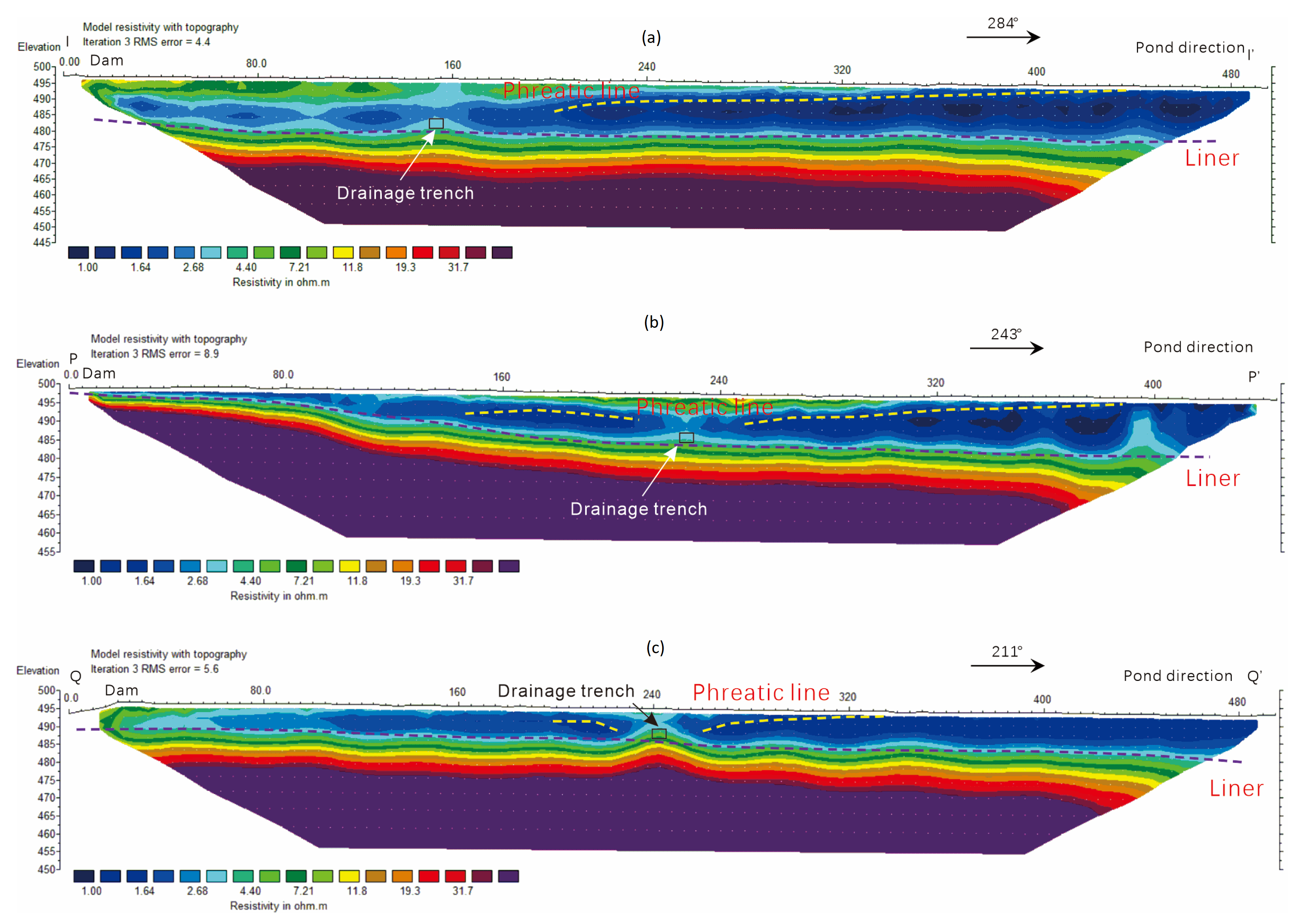
Figure 7 presents the results of the ERT survey conducted in the east and northeast area. All three profiles extended from the dam toward the decant pool, with the dam on the left side and areas closer to the decant pool on the right. Similar to other profiles, the subsurface could be divided into three layers based on resistivity values in the I−I’ and P−P’ profiles. The first layer consisted of shallow unsaturated tailings material. The thickness of the unsaturated zone varied at different locations due to the impact of drainage trenches in the pond and drainage pipes in the starter dam. The second layer comprised saturated tailings material. The saturated zone generally became thicker toward the decant pool. The maximum depth of phreatic lines reached 10 m. The third layer was the bottom geomembrane liner and natural sediments. For the I−I’ profile, the elevation of the geomembrane liner ranged from 477.8 m to 487.0 m. For the P−P’ profile, the elevation of the geomembrane liner was between 482.2 m and 496.8 m. For the Q−Q’ profile, the thickness of the accumulated tailings layer was only several meters thick. The elevation of the geomembrane liner on the Q−Q’ profile ranged from 483.8 m to 490.1 m.

4.3. Survey Results in the West Area

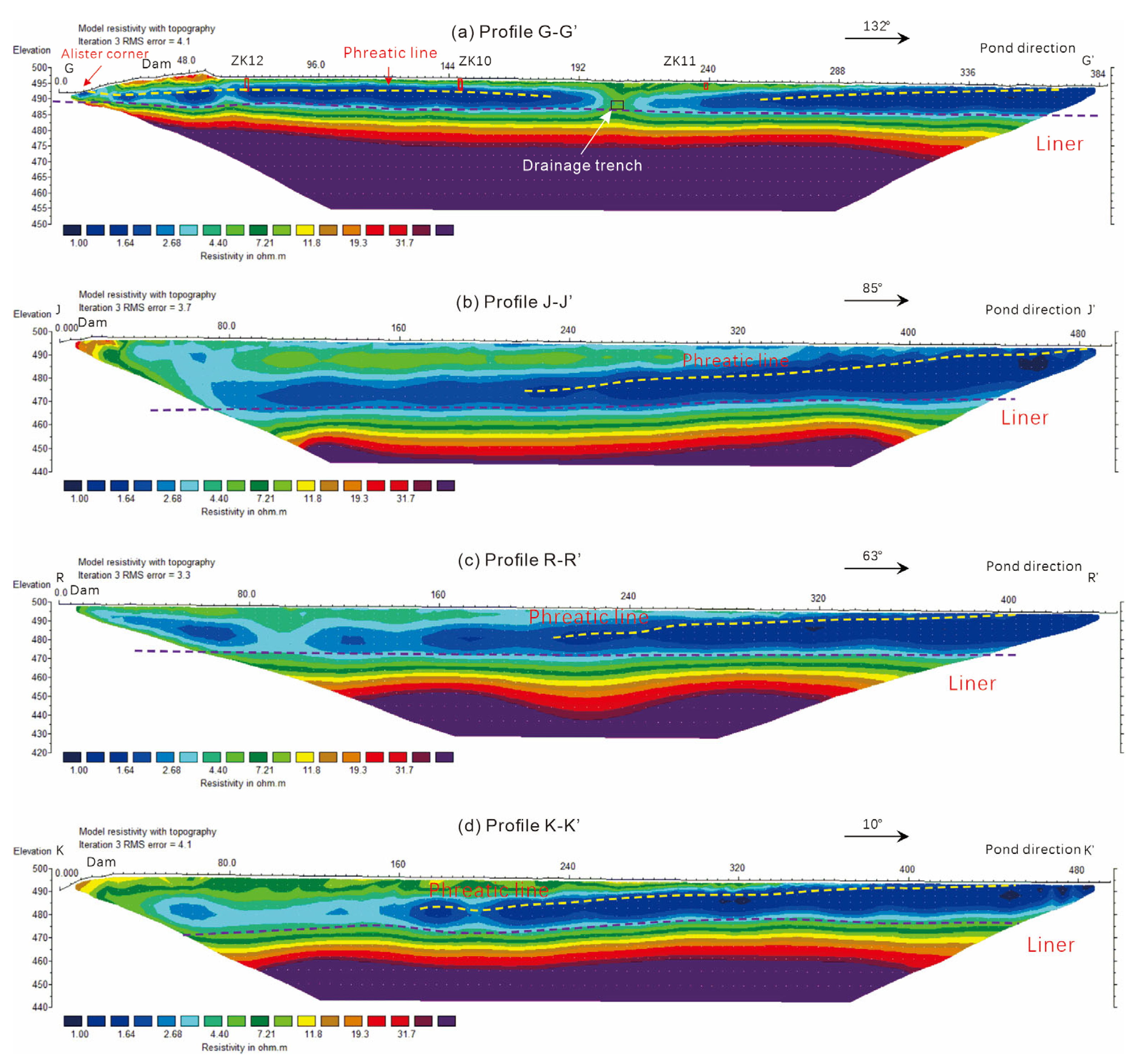
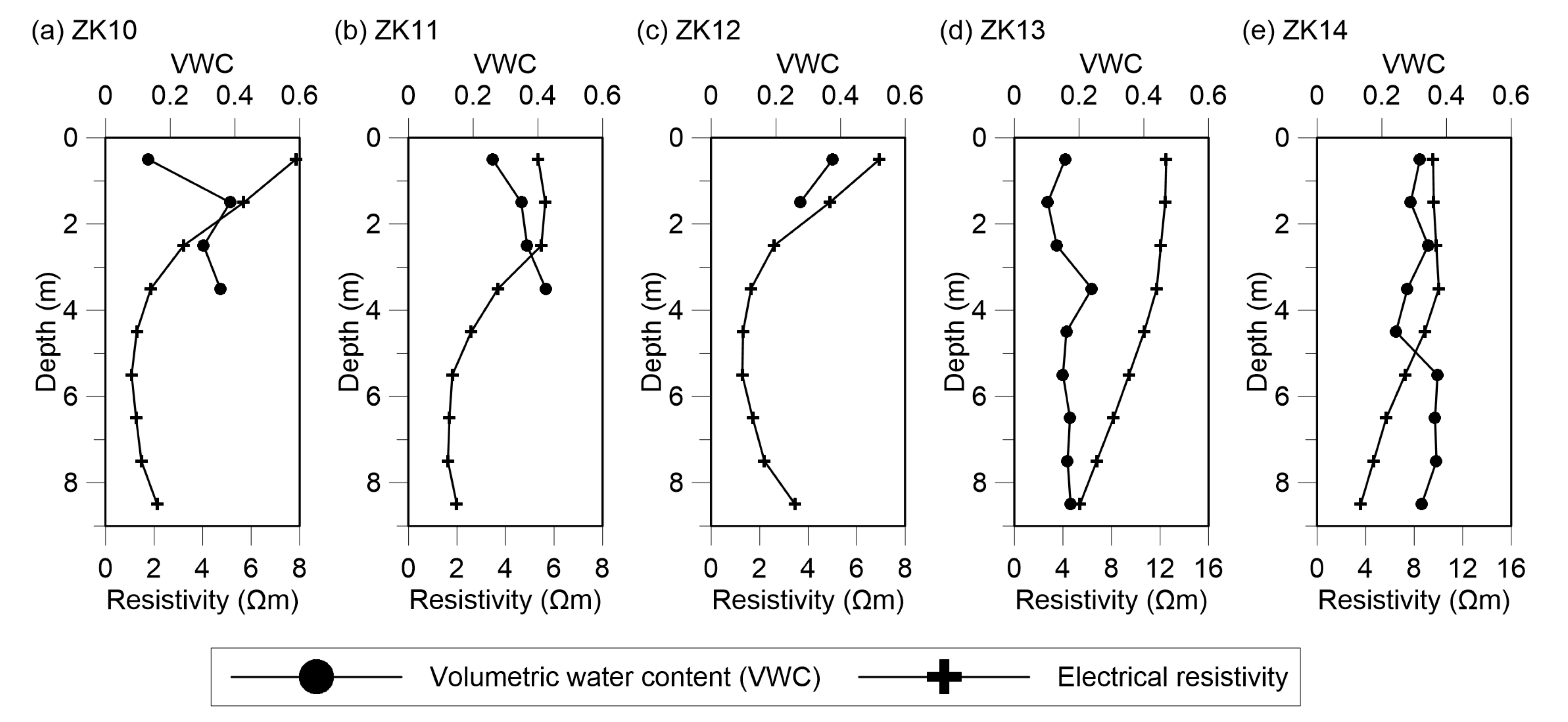
Figure 8 presents the results of the ERT survey conducted in the west area of the tailings dam. Figure 9 illustrates variations in electrical resistivity and volumetric water content at the boreholes. All ERT profiles extended from the dam toward the decant pool, with the dam on the left side and areas closer to the decant pool on the right. The tailings material could be divided into three layers from top to bottom. The first layer was the shallow unsaturated zone. In the dam area of profile J−J’, the thickness of the unsaturated zone exceeded 25 m, whereas in the dam area of profile G−G’, the thickness of the unsaturated zone was only roughly 5 m and gradually decreased toward the center of the reservoir. The volumetric water content in the unsaturated zone ranged from 0.13 to 0.42 and increased with depth (Figure 9a–c).
The second layer was the saturated zone. In the dam area of profile J−J’, the thickness of the saturated zone was relatively small but increased gradually toward the center of the reservoir, reaching a maximum thickness of over 20 m. In profile G−G’, the thickness of the saturated zone remained relatively stable, varying between 2 and 5 m. The profile G−G’ starting across the Alister corner (seepage) indicated that the low-resistivity zone was located at the same elevation and showed continuity. The third layer was the geomembrane liner. The elevation of the geomembrane liner on profile J−J’ was approximately 470 m, while in profile G−G’, the elevation of the geomembrane liner ranged from approximately 485 to 490 m.
The resistivity distribution of the profile R−R’ was similar to that of the profile K−K’. The subsurface can be divided into three layers based on resistivity values. The first layer consists of shallow unsaturated tailings material, with a thickness reaching more than 20 m near the dam body. The second layer comprises saturated tailings material, where the thickness of the saturated zone increases toward the decant pool. The resistivity results indicated the absence of a continuous saturated zone near the dam, suggesting that the drainage pipes effectively prevented the accumulation of seepage water. The third layer is the bottom geomembrane liner, with elevations ranging from 471.5 to 474.8 m for profile R−R’ and from 468.5 to 472.2 m for profile K−K’.
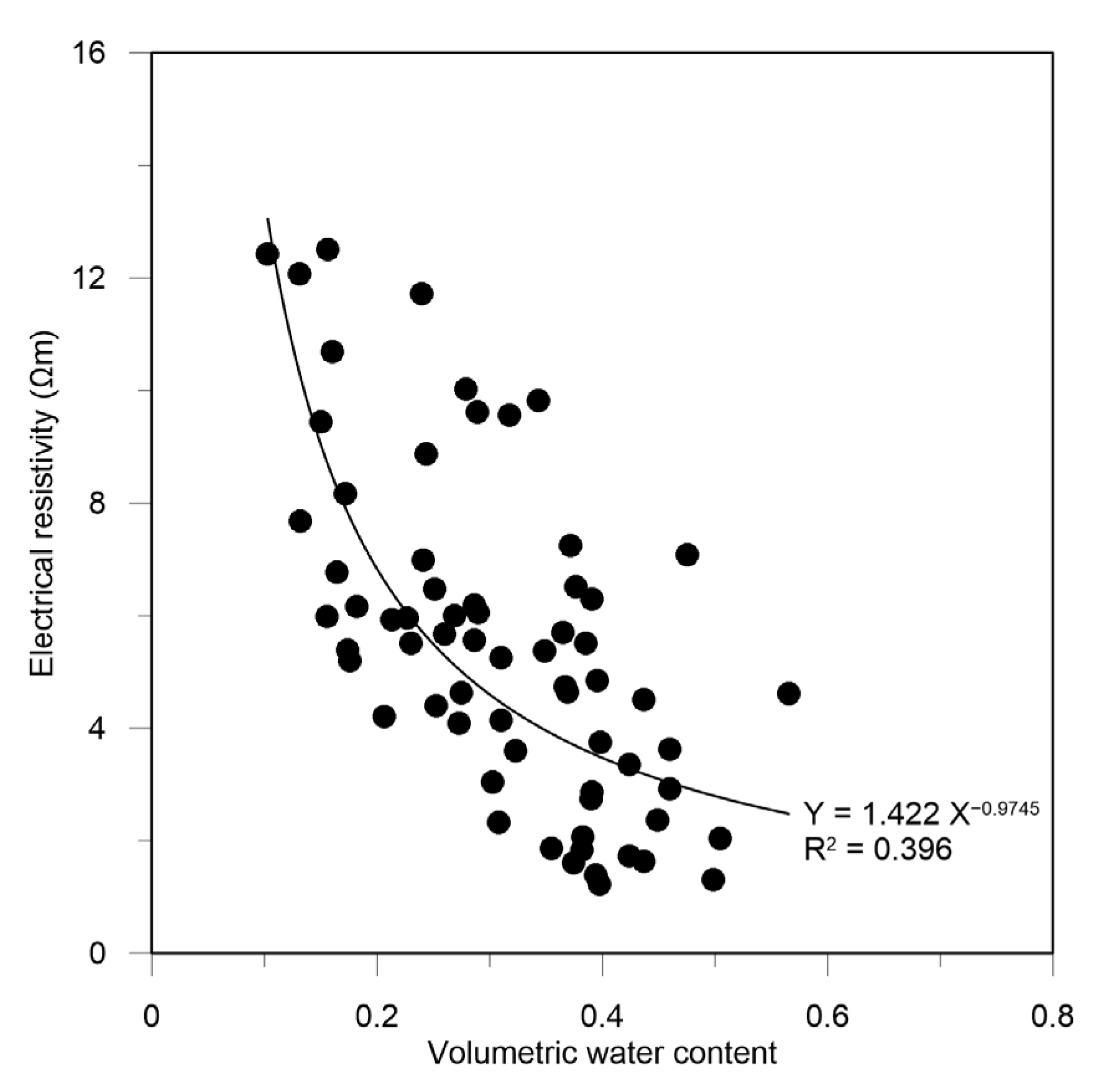
Figure 10 presents a comparison of the electrical resistivity and volumetric water content at boreholes. A power function was employed to fit this relationship. The results showed that electrical resistivity was inversely proportional to the volumetric water content. When the volumetric water content exceeds 0.5, the tailings material becomes fully saturated and the electrical resistivity drops below 1.6 Ωm.

4.4. Detection of Seepage Pathways

4.4.1. Seepage Analysis of the Lebusa Corner

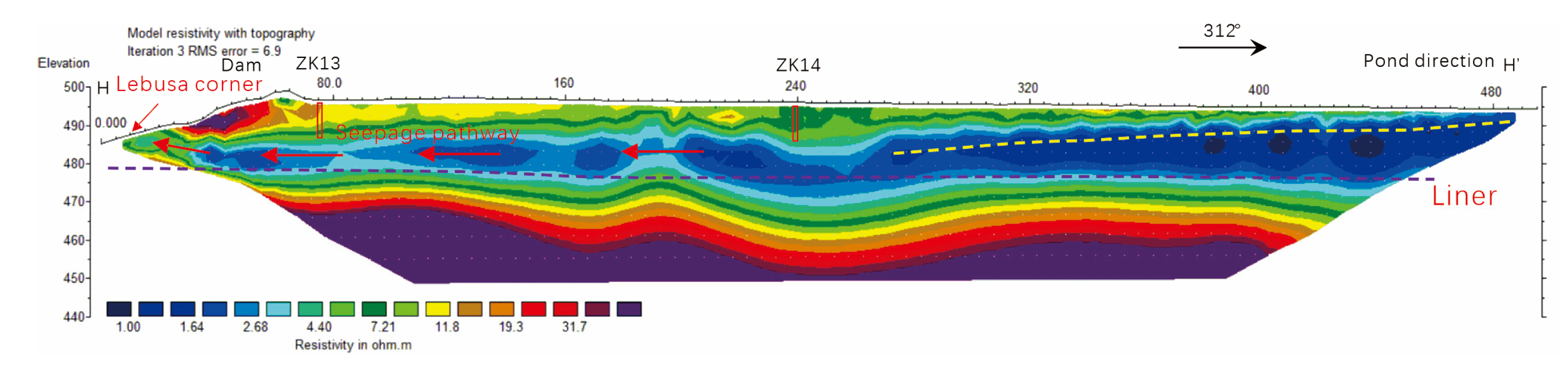
The Lebusa corner was located at the junction between the starter dam and the tailings embankment on the southeast side of the tailings dam (Figure 11). The H−H’ profile was established from the Lebusa corner toward the central decant pool, with an electrode spacing of 5 m and a total length of 495 m. The Schlumberger array configuration was used. Figure 11 presents the investigation results of the seepage pathway at the Lebusa corner. The red area on the left shows the shallow high-resistivity tailings embankment. This material is densely compacted and has low moisture content. As a result, its resistivity exceeds 20 Ωm. The subsurface resistivity distribution could also be divided into three layers: the unsaturated zone, the saturated zone, and the impermeable layer. In borehole ZK13 near the tailings embankment, the volumetric water content in the unsaturated zone was between 0.10 and 0.24 (Figure 9d). In borehole ZK14 near the center of the tailing pond, the volumetric water content increased to 0.29 and 0.37 (Figure 9e). The saturated zone (dark blue area) was generally continuous and stable, extending progressively from the Lebusa corner toward the decant pool. A significant low-resistivity zone was also present at depths of 10 to 20 m beneath the tailings embankment. The results indicate that the seepage source at the Lebusa corner was clarified water from the decant pool, and the seepage pathway was the saturated zone within the tailings pond.

4.4.2. Seepage Analysis of the Alister Corner

The Alister corner was located at the junction between the starter dam and the tailings embankment on the northwest side of the tailings pond (Figure 3). The G−G’ profile extended from the Alister corner toward the central decant pool. The G−G’ profile comprised an electrode spacing of 3 m and a total length of 387 m. The Wenner array configuration was used, and the investigation results are shown in Figure 8a.
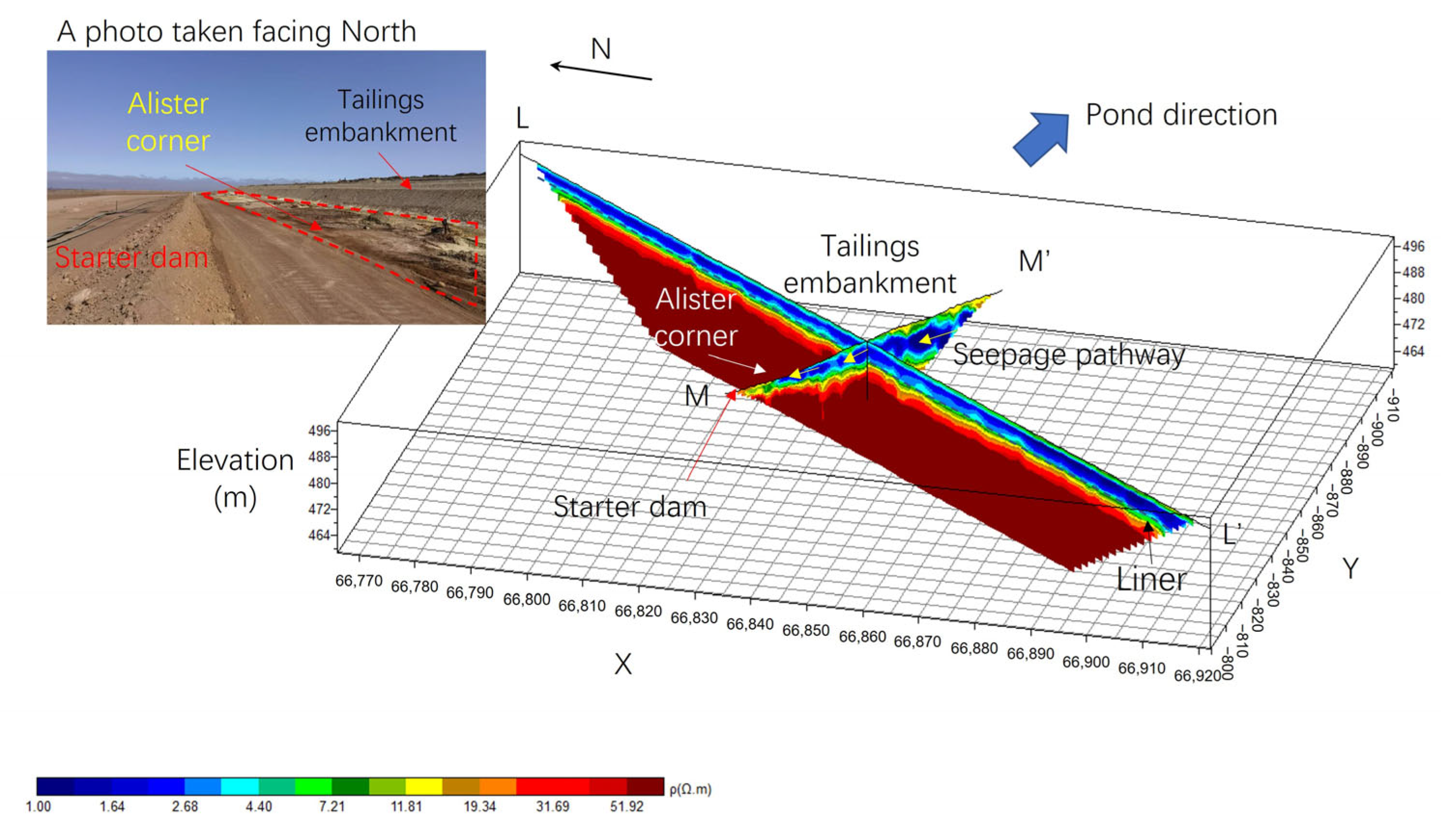
To further investigate the seepage pathway, the M−M’ and L−L’ profiles were established for detailed imaging. Figure 12 presents the three-dimensional investigation results of the seepage channel at the Alister corner. The M−M’ profile comprised an electrode spacing of 1 m and a total length of 59 m. The low-resistivity (dark blue) zone represents the saturated zone within the tailings pond. By comparing and analyzing these results with the G−G’ profile presented in Figure 8a, it can be concluded that the seepage source at the Alister corner was clarified water from the decant pool, and the seepage pathway was the saturated zone within the tailings pond.
The L−L’ profile was located along the southeast slope of the Alister corner seepage channel and was oriented perpendicularly to the M−M’ profile. A stable and continuous low-resistivity zone (blue) between elevations 490 and 492 m was identified as the seepage channel. Field investigations indicated that the seepage zone at the Alister corner extended over 400 m in length and ranged between 2 and 3 m in width.
The seepage mechanisms at the Lebusa and Alister corners were similar. Clarified water from the decant pool migrated through the saturated zone of the tailings pond. The water migrated along the base of the tailings embankment. Upon encountering the starter dam, the flow was impeded and subsequently emerged as seepage at the junction between the starter dam and the tailings embankment.

4.5. Infiltration Process of Water During the Deposition Process

TL-ERT of the E−E’ profile was conducted to analyze the infiltration process of water from the W13 slurry discharge outlet. During monitoring, the electrodes on the survey lines were fixed along the boundary between the inner side of the tailings embankment and the loose tailings. TL-ERT measurements were taken every 1 to 2 h. The results from different time periods were then analyzed and compared. A total of 13 sets of TL-ERT data were examined. The slurry discharge rate was approximately 2500 m3/h. Discharge through the W13 outlet lasted for 8.5 h, resulting in a total volume of approximately 21,250 m3 of slurry.
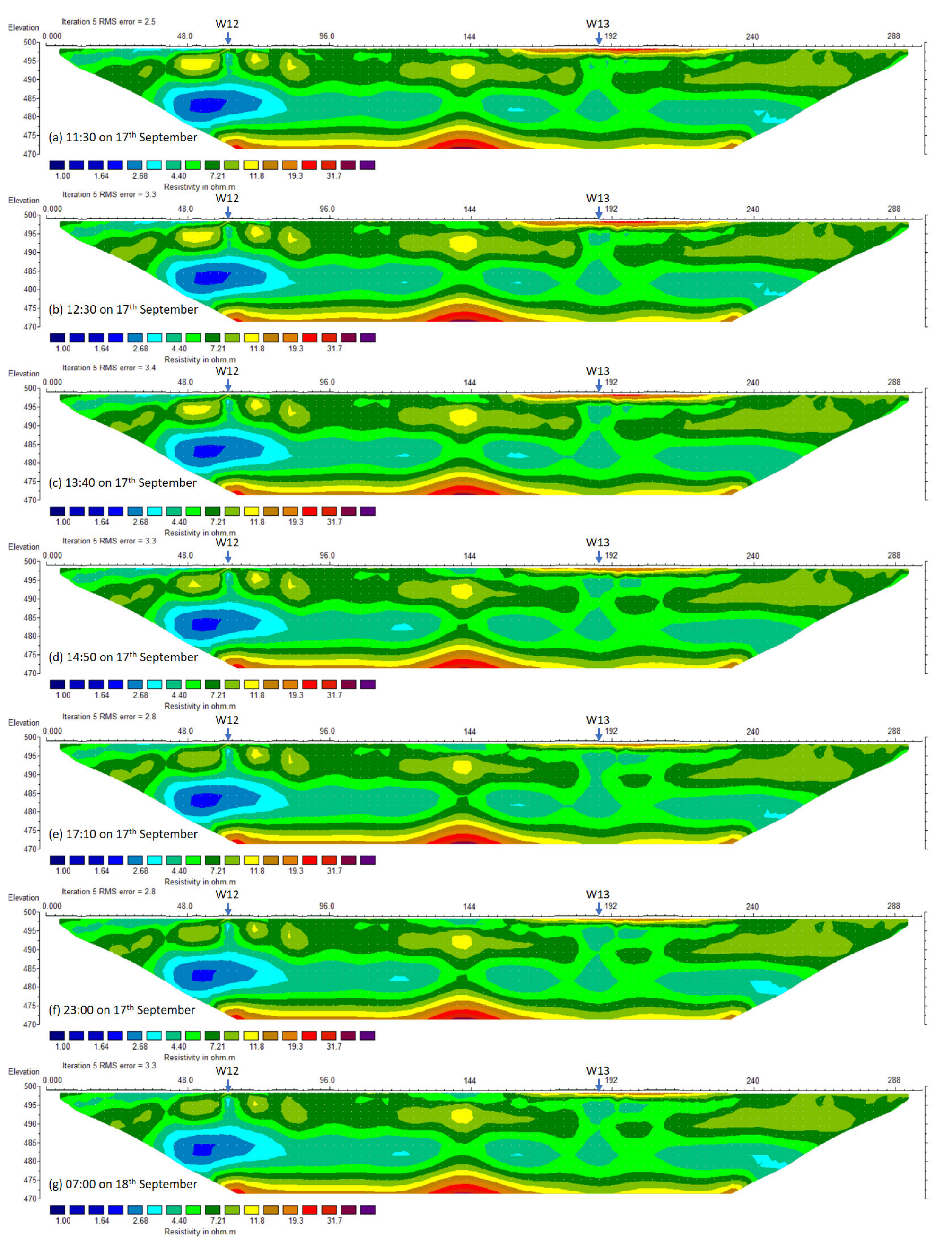
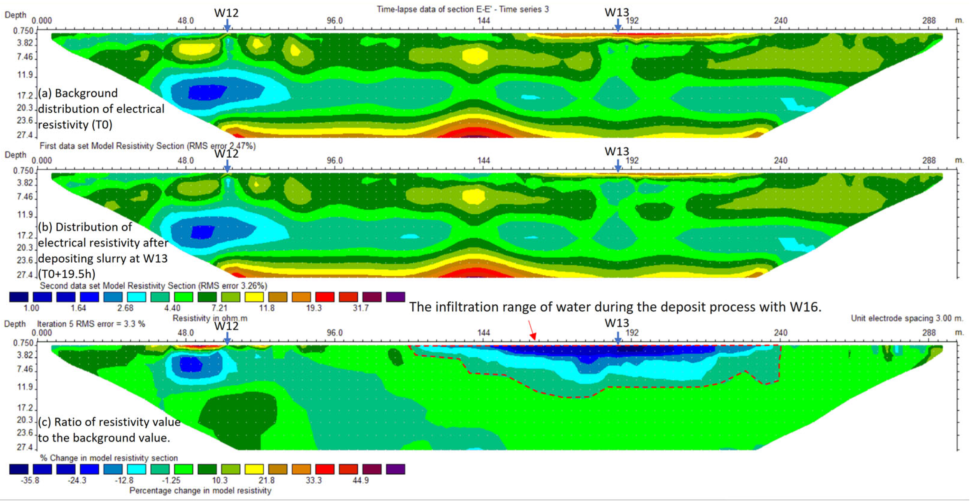
Figure 13 illustrates the monitoring results of TL-ERT during the deposition process at W13. Figure 13a represents the background values before the discharge began. Before the measurement, the W12 discharge outlet had been releasing tailings for 6 h. Water infiltration occurred around and beneath the W12 outlet, which was evident as a low-resistivity zone. The tailings material near the W13 discharge outlet was relatively dry, with surface resistivity exceeding 11 Ωm. Subsurface resistivity ranged between 4 and 6 Ωm. The distribution of resistivity generally paralleled the topographic contours, indicative of the stratified deposition of tailings materials.
Figure 13b–g present the resistivity distribution during the discharge process. At 11:30 a.m. on September 17, the W12 discharge outlet was closed, and the W13 discharge outlet was opened. The resistivity in the area surrounding W13 gradually decreased. The orange areas representing higher resistivity in the shallow layers started to diminish, while the green areas indicating lower resistivity (5~6 Ωm) in deeper layers began to expand. Centered around W13, moisture spread both horizontally and vertically. By 20:00 on September 17, the W13 discharge outlet was closed. The resistivity in the vicinity of W13 reached a relatively stable state with minimal overall changes.
Figure 14 illustrates variations in electrical resistivity during the deposition process. Figure 14a represents the background values before the discharge began. Figure 14b depicts the distribution of electrical resistivity 19.5 h after the start of slurry deposition at the W13 port. Figure 14c presents the ratio of the final resistivity values to the background values, with blue areas indicating a decrease in resistivity and an increase in moisture content. The horizontal extent of increased moisture due to the discharge process from W13 was approximately 60 m, and the vertical extent was roughly 10 m.

5. Conclusions

Due to its capacity for non-invasive measurement and sensitivity to conductive acid mine drainage, ERT is an effective complementary tool for seepage detection in the TSF. In this study, ERT was used to detect the internal structure and phreatic surface of the TSF of Husab Mine. The seepage pathways were identified, with the seepage mechanisms subsequently analyzed. Lastly, TL-ERT was conducted to monitor the infiltration of water during the deposition process.
Our results demonstrate that the tailings sediments were divided into three layers based on resistivity values. The first layer consisted of shallow unsaturated tailings material with resistivity generally ranging between 1.6 Ωm and 12 Ωm. The volumetric water content of the unsaturated tailings exhibited an increasing trend with depth. The second layer comprised saturated tailings material with resistivity values ranging between 0.8 Ωm and 1.6 Ωm. The volumetric water contents at the phreatic surface ranged from 0.4 to 0.5. The thickness of the saturated zone gradually increased from the dam toward the decant pool. The depth of the phreatic surface was more than 17 m near the tailings dam. The phreatic surface shoaled toward the decant pool. The third layer consisted of the bottom natural sediments and a geomembrane liner.
The Lebusa corner (seepage) was located on the southeast side of the TSF. The Alister corner (seepage) was located on the northwest side of the TSF. Seepage occurred because clarified water from the decant pool migrated through the saturated zone of the tailings pond along the base of the tailings embankment. Upon encountering the starter dam, the water was impeded and subsequently emerged as seepage at the junction between the starter dam and the tailings embankment. TL-ERT monitoring results show that the horizontal extent of increased moisture was approximately 60 m, and the vertical extent was roughly 10 m due to the deposition process. A focus of future studies will be to evaluate the stability of the TSF based on the survey results.

Supplementary Materials

The following supporting information can be downloaded at: https://www.mdpi.com/article/10.3390/min16070723/s1.

Author Contributions

Conceptualization, Q.Z.; Methodology, C.L.; Validation, X.L.; Software and Visualization, C.L.; Writing—Original Draft Preparation, X.L.; Writing—review and editing, C.L.; Investigation, X.L., J.Y. (Juan Yang) and Z.L.; Supervision, M.X.; Project administration, J.Y. (Jiake Yang). All authors have read and agreed to the published version of the manuscript.

Funding

This research was supported by the project “provision of scientific research on dynamic seepage development at Husab TSF” (SU-2025-0098) funded by Swakop Uranium (PTY) LTD.

Data Availability Statement

The original contributions presented in this study are included in the article/Supplementary Material. Further inquiries can be directed to the corresponding author.

Acknowledgments

The authors are grateful to John Moody, Eva Shinyongo, Nicolaas Van Der Westhuizen, Canqi Chen, Sizwe Ngonomo, Popyeni Shikongo, and others for their invaluable support and assistance in the field investigation performed in this study. We thank the three referees for their invaluable review of our manuscript.

Conflicts of Interest

Xiao Li, Juan Yang and Jiake Yang are employees of Uranium Resources Co., Ltd., China General Nuclear Power Corporation. The paper reflects the views of the scientists and not the company.

Abbreviations

The following abbreviations are used in this manuscript:
ERTElectrical resistivity tomography
TL-ERTTime-lapse electrical resistivity tomography

References

  1. Franks, D.M.; Stringer, M.; Torres-Cruz, L.A.; Baker, E.; Valenta, R.; Thygesen, K.; Matthews, A.; Howchin, J.; Barrie, S. Tailings facility disclosures reveal stability risks. Sci. Rep. 2021, 11, 5353. [Google Scholar] [CrossRef] [PubMed]
  2. Azam, S.; Li, Q. Tailings dam failures: A review of the last one hundred years. Geotech. News 2010, 28, 50–54. [Google Scholar]
  3. Hudson-Edwards, K.A.; Kemp, D.; Torres-Cruz, L.A.; Macklin, M.G.; Brewer, P.A.; Owen, J.R.; Franks, D.M.; Maerquis, E.; Thomas, C.J. Tailings storage facilities, failures and disaster risk. Nat. Rev. Earth Environ. 2024, 5, 612–630. [Google Scholar] [CrossRef]
  4. Piciullo, L.; Storrøsten, E.B.; Liu, Z.; Nadim, F.; Lacasse, S. A new look at the statistics of tailings dam failures. Eng. Geol. 2022, 303, 106657. [Google Scholar] [CrossRef]
  5. Clarkson, L.; Williams, D. An overview of conventional tailings dam geotechnical failure mechanisms. Min. Metall. Explor. 2021, 38, 1305–1328. [Google Scholar] [CrossRef]
  6. Silva Rotta, L.H.; Alcântara, E.; Park, E.; Negri, R.G.; Lin, Y.N.; Bernardo, N.; Gonçalves Mendes, T.S.; Souza Filho, C.R. The 2019 Brumadinho tailings dam collapse: Possible cause and impacts of the worst human and environmental disaster in Brazil. Int. J. Appl. Earth Obs. 2020, 90, 102119. [Google Scholar] [CrossRef]
  7. Wang, G.; Hu, B.; Tian, S.; Ai, M.; Liu, W.; Kong, X. Seepage field characteristic and stability analysis of tailings dam under action of chemical solution. Sci. Rep. 2021, 11, 4073. [Google Scholar] [CrossRef] [PubMed]
  8. Fu, B.; Pei, J.; Ji, H. Numerical simulation of three-dimensional seepage field in a tailing pond under multiple operating conditions. Sci. Rep. 2024, 14, 28027. [Google Scholar] [CrossRef] [PubMed]
  9. Binley, A.; Slater, L. Resistivity and Induced Polarization: Theory and Application to the Near-Surface Earth; Cambridge University Press: Cambridge, UK, 2020; pp. 215–262. [Google Scholar]
  10. Singh, K.K.K.; Bharti, A.K.; Pal, S.K.; Prakash, A.; Saurabh Kumar, R.; Singh, P.K. Delineation of fracture zone for groundwater using combined inversion technique. Environ. Earth Sci. 2019, 78, 110. [Google Scholar] [CrossRef]
  11. Srivastava, S.; Vikash, V.; Pal, S.K.; Kumar, S.; Mondal, S.; Bhaumik, A.K. Integrated geophysical approach for bauxite exploration in Bimarla mine, Lohardaga, Jharkhand, India. Min. Metall. Explor. 2025, 42, 2441–2457. [Google Scholar] [CrossRef]
  12. Mondal, S.; Pal, S.K.; Guha, A.; Kumar, R. Multi-Modal geophysical characterization of chromite deposits in the Sittampundi igneous layered complex, Tamil Nadu, India. Pure Appl. Geophys. 2025, 182, 3139–3166. [Google Scholar] [CrossRef]
  13. Srivastava, S.; Kumar, R.; Pal, S.K.; Bhattacharjee, R.M. Mapping of old coal mine galleries near railway track using electrical resistivity tomography and magnetic approaches in Tundu, Jogidih Colliery, Jharia Coalfield, India. J. Earth Syst. Sci. 2024, 133, 57. [Google Scholar] [CrossRef]
  14. Li, G.; Zhang, H.; Li, M.; Shen, Z.; Tian, A.; Wang, L. Study on coal wall spalling mechanism of large mining height working face based on folding mutation theory. Sci. Rep. 2026, 16, 15277. [Google Scholar] [CrossRef] [PubMed]
  15. Kumar, R.; Pal, S.K.; Gupta, P.K. Water seepage mapping in an underground coal-mine barrier using self-potential and electrical resistivity tomography. Mine Water Environ. 2021, 40, 622–638. [Google Scholar] [CrossRef]
  16. Bharti, A.K.; Singh, S.K.; Pal, S.K.; Singh, K.K.K.; Prakash, A.; Bhattacharjee, R.; Kumar, L. Electrical resistivity tomography technique coupled with numerical modelling: A case study for stability analysis. Geophys. Prospect. 2023, 71, 1368–1384. [Google Scholar] [CrossRef]
  17. Li, Z.; Ren, H.; Wang, W.; Du, F.; Huang, Y.; Cao, Z.; Wang, L. Multi-factor coupled numerical simulation and sensitivity analysis of hysteresis water inundation induced by the activation of small faults in the bottom plate under the influence of mining. Appl. Sci. 2026, 16, 1051. [Google Scholar] [CrossRef]
  18. Ali, M.A.H.; Mewafy, F.M.; Qian, W.; Alshehri, F.; Almadani, S.; Aldawsri, M.; Aloufi, M.; Saleem, H.A. Mapping leachate pathways in aging mining tailings pond using electrical resistivity tomography. Minerals 2023, 13, 1437. [Google Scholar] [CrossRef]
  19. Córdova, L.; Moya, A.; Comte, D.; Bravo, I. Methodology for the identification of moisture content in tailings dam walls based on electrical resistivity tomography technique. Minerals 2024, 14, 760. [Google Scholar] [CrossRef]
  20. Lghoul, M.; Teixidó, T.; Peña, P.A.; Hakkou, R.; Kchikach, A.; Guérin, R.; Jaffal, M.; Zouhri, L. Electrical and seismic tomography used to image the structure of a tailings pond at the abandoned Kettara mine, Morocco. Mine Water Environ. 2012, 31, 53–62. [Google Scholar] [CrossRef]
  21. Oliveira, L.A.; Braga, M.A.; Prosdocimi, G.; de Souza Cunha, A.; Santana, L.; da Gama, F. Improving tailings dam risk management by 3D characterization from resistivity tomography technique: Case study in São Paulo—Brazil. J. Appl. Geophys. 2023, 210, 104924. [Google Scholar] [CrossRef]
  22. Martínez, J.; Mendoza, R.; Rey, J.; Sandoval, S.; Hidalgo, M.C. Characterization of tailings dams by electrical geophysical methods (ERT, IP): Federico mine (La Carolina, Southeastern Spain). Minerals 2021, 11, 145. [Google Scholar] [CrossRef]
  23. Gabarrón, M.; Martínez-Pagán, P.; Martínez-Sequra, M.A.; Bueso, M.C.; Martínez- Martínez, S.; Faz, Á.; Acosta, J.A. Electrical resistivity tomography as a support tool for physicochemical properties assessment of near-surface waste materials in a mining tailing pond (El Gorguel, SE Spain). Minerals 2020, 10, 559. [Google Scholar] [CrossRef]
  24. Martínez-Pagán, P.; Gómez-Ortiz, D.; Martín-Crespo, T.; Martín-Velázquez, S.; Martínez-Sequra, M. Electrical resistivity imaging applied to tailings ponds: An overview. Mine Water Environ. 2021, 40, 285–297. [Google Scholar] [CrossRef]
  25. Dimech, A.; Cheng, L.Z.; Chouteau, M.; Chambers, J.; Uhlemann, S.; Wilkinson, P.; Meldrum, P.; Mary, B.; Fabien-Ouellet, G.; Isabelle, A. A review on applications of time-lapse electrical resistivity tomography over the last 30 years: Perspectives for Mining Waste Monitoring. Surv. Geophys. 2022, 43, 1699–1759. [Google Scholar] [CrossRef] [PubMed]
  26. Rucker, D.F.; Crook, N.; Winterton, J.; McNeill, M.; Baldyga, C.A.; Noonan, G.; Fink, J.B. Real-time electrical monitoring of reagent delivery during a subsurface amendment experiment. Near Surf. Geophys. 2014, 12, 151–163. [Google Scholar]
  27. Mainali, G.; Nordlund, E.; Knutsson, S.; Thunehed, H. Tailings dams monitoring in Swedish mines using self-potential and electrical resistivity methods. Electron. J. Geotech. Eng. 2015, 20, 5859–5875. [Google Scholar]
  28. Hester, E.T.; Little, K.L.; Buckwalter, J.D.; Zipper, C.E.; Burbey, T.J. Variability of subsurface structure and infiltration hydrology among surface coal mine valley fills. Sci. Total Environ. 2019, 651, 2648–2661. [Google Scholar] [CrossRef] [PubMed]
  29. Mendelsohn, J.; Jarvis, A.; Roberts, C.; Rebertson, T. Atlas of Namibia. A Portrait of the Land and its People; David Philip Publishers: Cape Town, South Africa, 2002; pp. 68–93. [Google Scholar]
  30. Loke, M.H. Tutorial: 2-D and 3-D Electrical Imaging Surveys; Geotomo Software: Gelugor, Malaysia, 2014; p. 127. [Google Scholar]
  31. Ellis, R.G.; Oldenburg, D.W. Applied geophysical inversion. Geophys. J. Int. 1994, 116, 5–11. [Google Scholar] [CrossRef]
  32. Loke, M.H.; Dahlin, T.; Rucker, D.F. Smoothness-constrained time-lapse inversion of data from 3-D resistivity surveys. Near Surf. Geophys. 2014, 12, 5–24. [Google Scholar]
  33. Loke, M.H. Time-lapse resistivity imaging inversion. In Proceedings of the 5th Meeting of the Environmental and Engineering Geophysical Society European Section Proceedings, Budapest, Hungary, 6–9 September 1999. [Google Scholar]
  34. ASTM D2216-19; ASTM Standard Test Methods for Laboratory Determination of Water (Moisture) Content of Soil and Rock by Mass. ASTM International: West Conshohocken, PA, USA, 2019.
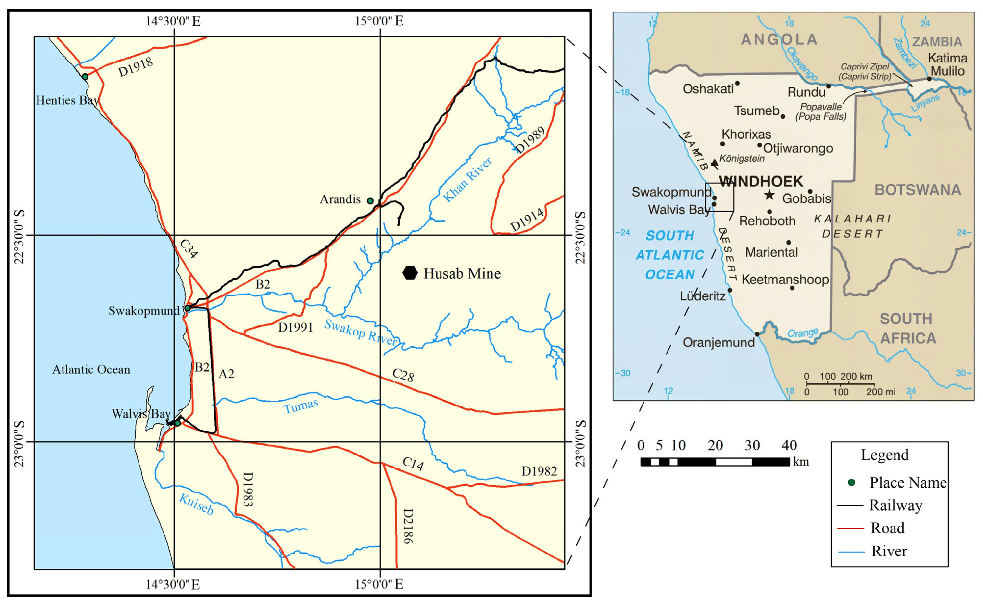
Figure 1. Location of the Husab Mine.
Minerals 16 00723 g001
Figure 2. Layout of the Husab Mine.
Minerals 16 00723 g002
Figure 3. Layout of TSF and ERT profiles. A total of 16 ERT profiles were acquired to detect the structure and seepage pathways of the tailings pond. The Lebusa corner (seepage) is located on the southeast side of the tailings dam. The length of seepage exceeds 300 m at the Lebusa corner. The Alister corner (seepage) is located on the northwest side of the tailings dam.
Minerals 16 00723 g003
Figure 4. Schematic cross-section of the tailings dam and its seepage drainage system.
Minerals 16 00723 g004
Figure 5. ERT results in the southeast area. (a) Profile A−A’; (b) Profile B−B’; (c) Profile C−C’; (d) Profile D−D’. The yellow dashed lines denote the estimated phreatic lines, while the purple dashed lines indicate the liner. The number of iterations and the corresponding RMS values are displayed in the upper left corner.
Minerals 16 00723 g005
Figure 6. Variations in the resistivity and volumetric water content at boreholes. (a) Borehole ZK2; (b) Borehole ZK3; (c) Borehole ZK4; (d) Borehole ZK5; (e) Borehole ZK7. The resistivity data were derived from the inversion results of ERT profiles. Boreholes ZK2, ZK3, ZK4, and ZK5 were located on the B−B’ profile, whereas borehole ZK7 was situated on the C−C’ profile.
Minerals 16 00723 g006
Figure 7. ERT results in the east and northeast areas. (a) Profile I−I’; (b) Profile P−P’; (c) Profile Q−Q’. The yellow dashed lines denote the estimated phreatic lines, while the purple dashed lines indicate the liner. The number of iterations and the corresponding RMS values are displayed in the upper left corner.
Minerals 16 00723 g007
Figure 8. ERT results in the west area. (a) Profile G−G’; (b) Profile J−J’; (c) Profile R−R’; (d) Profile K−K’. The yellow dashed lines denote the estimated phreatic lines, while the purple dashed lines indicate the liner. The number of iterations and the corresponding RMS values are displayed in the upper left corner.
Minerals 16 00723 g008
Figure 9. Variations in electrical resistivity and volumetric water content at boreholes. (a) Borehole ZK10; (b) Borehole ZK11; (c) Borehole ZK12; (d) Borehole ZK13; (e) Borehole ZK14. The resistivity data were derived from the inversion results of ERT profiles. Boreholes ZK11, ZK12, and ZK13 were located on the G−G’ profile, while boreholes ZK13 and ZK14 were situated on the H−H’ profile.
Minerals 16 00723 g009
Figure 10. Comparison between the electrical resistivity and volumetric water content at boreholes. The black dots indicate the sampling points at boreholes. The black line represents the fitted curve. The fitting formula and the coefficient of determination are also displayed.
Minerals 16 00723 g010
Figure 11. ERT results of the profile H−H’ close to the Lebusa corner. The yellow dashed line denotes the estimated phreatic line, while the purple dashed line indicates the liner.
Minerals 16 00723 g011
Figure 12. ERT results of the Alister corner.
Minerals 16 00723 g012
Figure 13. Monitoring results of TL-ERT during the deposition process at the W13 outlet. (a) Result at 11:30 on 17th September; (b) Result at 12:30 on 17th September; (c) Result at 13:40 on 17th September; (d) Result at 14:50 on 17th September; (e) Result at 17:10 on 17th September; (f) Result at 23:00 on 17th September; (g) Result at 07:00 on 18th September. Note that the W12 outlet was closed and the W13 outlet was opened simultaneously at 11:30 a.m. on 17th September, 2025. Discharge through W13 outlet lasted for 8.5 h and terminated at 8:00 p.m. on 17th September, 2025. The significant changes in resistivity occurred around and beneath the W13 outlet.
Minerals 16 00723 g013
Figure 14. Variations in electrical resistivity during the deposition process. (a) Background distribution of electrical resistivity before deposition. (b) Distribution of electrical resistivity 19.5 h after the start of slurry deposition at the W13 port, with a total of 8.5 h of slurry deposition. (c) Ratio of resistivity value to the background value.
Minerals 16 00723 g014
Table 1. Parameter settings of ERT profiles.
No.Profile
Name
Electrode
Spacing (m)
Total Number
of Electrodes
Profile
Length (m)
Array TypeMaximum
Spacing Factor
Data Number
1A−A’3140417Wenner252480
2B−B’3180537Wenner253435
3C−C’3180537Wenner253511
4D−D’3160477Wenner253011
5E−E’3100297Schlumberger251825/set, 13 sets
6F−F’3150447Schlumberger254323
7G−G’3130387Wenner252268
8H−H’5100495Schlumberger251825
9I−I’5100495Schlumberger251825
10J−J’5100495Wenner302040
11K−K’5100495Wenner302040
12L−L’2100198Wenner251825
13M−M’16059Wenner25825
14P−P’590445Wenner25990
15Q−Q’5100495Wenner251125
16R−R’590445Wenner251275
Total18806721 56,523
Disclaimer/Publisher’s Note: The statements, opinions and data contained in all publications are solely those of the individual author(s) and contributor(s) and not of MDPI and/or the editor(s). MDPI and/or the editor(s) disclaim responsibility for any injury to people or property resulting from any ideas, methods, instructions or products referred to in the content.