Aeromagnetic Characterisation of the Breccia Zone at Machanur, Dharwar Craton

Abstract

High-resolution aeromagnetic data are analysed using data transformation and enhancement techniques, including Reduction to the Pole (RTP), First Vertical Derivative (FVD), Tilt Derivative (TDR), and Total Horizontal Derivative (THDR) and Upward Continuation (UC), along with spectral, 2D and 3D modelling. This approach aims to characterise the subsurface architecture of the Shear Zone associated with breccia near Machanur in the Dharwar Craton, Southern India. Qualitative analysis indicates that an ENE-WSW-trending magnetic low, measuring 300 nT and 7 km by 0.7 km, is identified in this zone and exhibits magnetic remanence. It is associated with NW-SE-, NE-SW-, E-W-, NNE-SSW-, and ENE-WSW-trending magnetic lineations. The Spectral, 2D and 3D modelling reveals that the average depth extension of the breccia zone is ~400 m. Therefore, it is possible that a distinct magnetic marker zone is present, extending down to an average depth of 400 m in the breccia zone, and it is structurally controlled. In conjunction with previous geological, petrological, and borehole information, with present analysis, mineralisation is noted at a depth greater than 350 m, particularly in the form of sulphide veins associated with chalcopyrite, pyrite, covellite, chalcocite, cuprite, bornite, and influenced by hydrothermal activity.

1. Introduction

‘Breccia’ is a rock composed of large angular/sharp corners of broken fragments of minerals cemented together by a fine-grained matrix and formed by igneous, sedimentary, and tectonic processes. Igneous-to-hydrothermal chert, fault, collapse, seismic, and impact are the available breccia types. These are associated with exogenic, endogenic, supergenic, and submarine ore environments. Mammoth in Arizona, Bajo de la Alumbrera in Argentina, and Naruo in Tibet [1,2,3] are examples of identified breccia zones in various parts of the world. In the Indian region, breccia zones are mapped in parts of Nuasahi, Odisha [4,5], the Cuddapah Basin [6], and the Bundelkhand Gneissic Complex [7]. The application of an understanding of Breccia zones implies an understanding of depositional settings, geodynamic evaluation and tectonic events. The study of impact breccias may also provide clues about the impact process of planetary bodies [8].

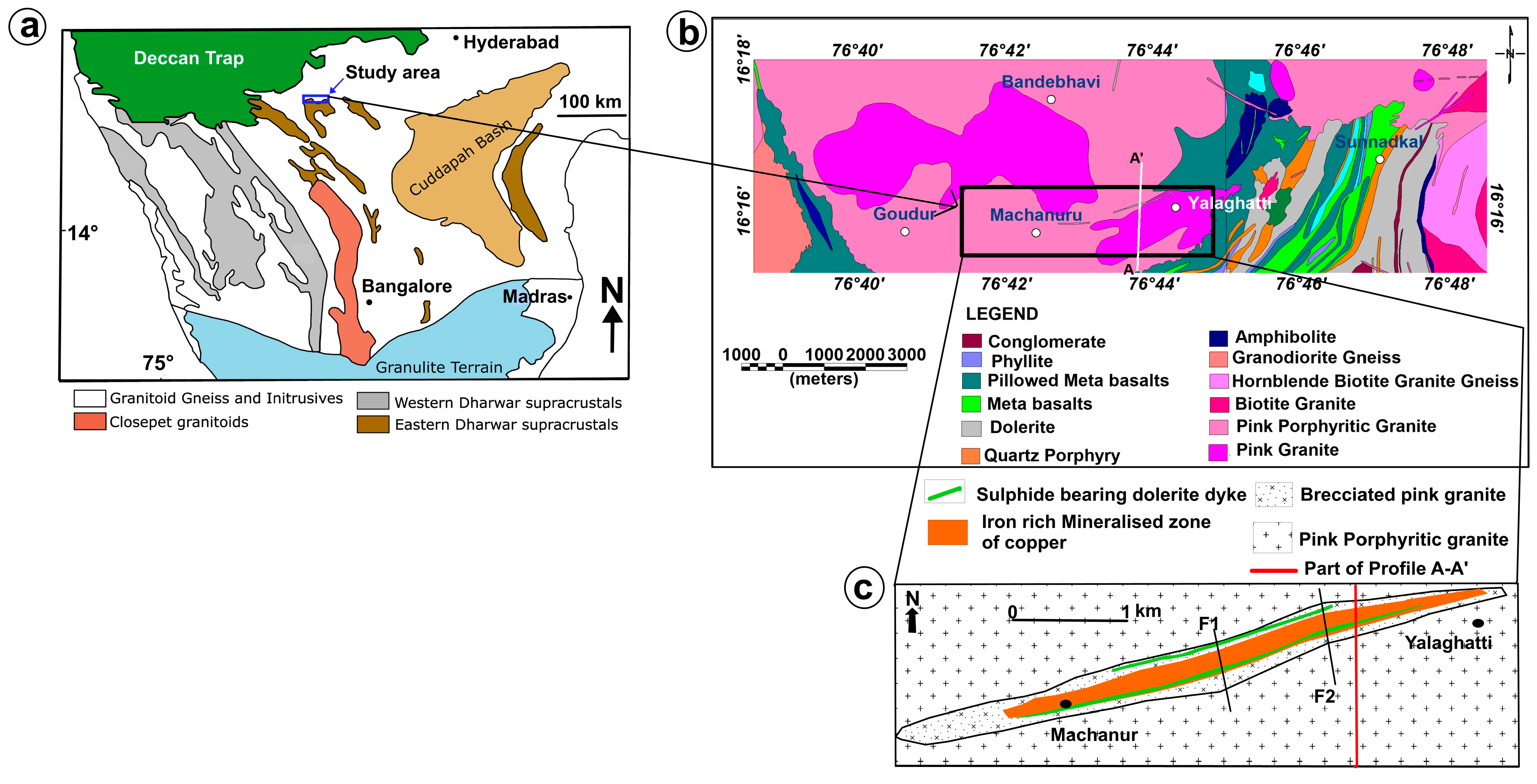
In previous work, refs. [9,10,11] have conducted extensive geological, petrological, and borehole studies at the Machanur block, Raichur, Karnataka in Dharwar Craton (Figure 1a), which identified Cu-Au and REE mineralisation at the breccia zone associated with a 400–500 m width brittle to ductile shear zone (Figure 1b). The identified breccia zone is 5 km long and striking in ENE to WSW with a width of 50–150 m (Figure 1c). Further, dolerite dykes are also mapped parallel to these shear zones, which are associated with mineralisation.

An intensive hydrothermal activity is identified along the breccia zone and it is faulted, consisting of angular granite clasts with a subordinate matrix, and it is cemented by quartz, iron oxides. It is surrounded by granite and granitoids, including closepet granite, characterised by quartz, chlorite, and iron oxide veins. The disseminated sulphide mineralisation is identified in the form of veins associated with chalcopyrite, pyrite, covellite, chalcocite, cuprite, and bornite. A considerable amount of gold is also reported from the boreholes, with a maximum of 4.4 g/tonne associated with chlorite hematite alteration zones and quartz carbonate veins. The borehole lithology >350 m also indicated the presence of mineralisation.

The present study focuses on the analysis of aeromagnetic data over the identified breccia zone in the Machanur block and to understand the magnetic characteristics of the breccia zone and its associated environment (comprising granite and the granitoid suite of closepet granite, parallel to the Krishna lineament, associated with mafic dykes and faulting). The magnetic technique is one of the geophysical tools used to map gold mineralisation associated with breccia zones, helping to vividly define fault zones that are often intricately linked to breccia formation and mineralisation [14,15].

Aeromagnetic data have proven to be a valuable tool for mineral exploration, as they enable the detection of subsurface structures, lithological contacts, and concealed intrusions that often host or control copper mineralisation [16,17]. Various derivative techniques, including First Vertical Derivative (FVD), Tilt Derivative (TDR), Analytic Signal (AS), and Total Horizontal Derivative (THDR), enhance subtle features in aeromagnetic data, allowing for the delineation of fault systems, dyke swarms, and alteration zones associated with mineralisation [18,19]. The integration of aeromagnetic interpretation with geological and structural data has successfully delineated mineralised zones in many Precambrian terrains globally and in India [20].

The present study area, Machanur, is a favourable geological environment for copper, gold, and REE mineralisation, characterised by greenstone sequences, mafic intrusions, and shear zones. However, due to a lack of detailed geophysical exploration, the subsurface structural controls on mineralisation remain poorly understood. This study aims to understand concealed geological structures, identify prospective copper-bearing zones, and characterise the associated structural framework controlling mineralisation using aeromagnetic anomalies. Here, we have analysed the aeromagnetic data using qualitative (FVD, TDR, THDR, and RTP), semi-quantitative (Spectral), and quantitative techniques (2D and 3D depth modelling).

2. Materials and Methods

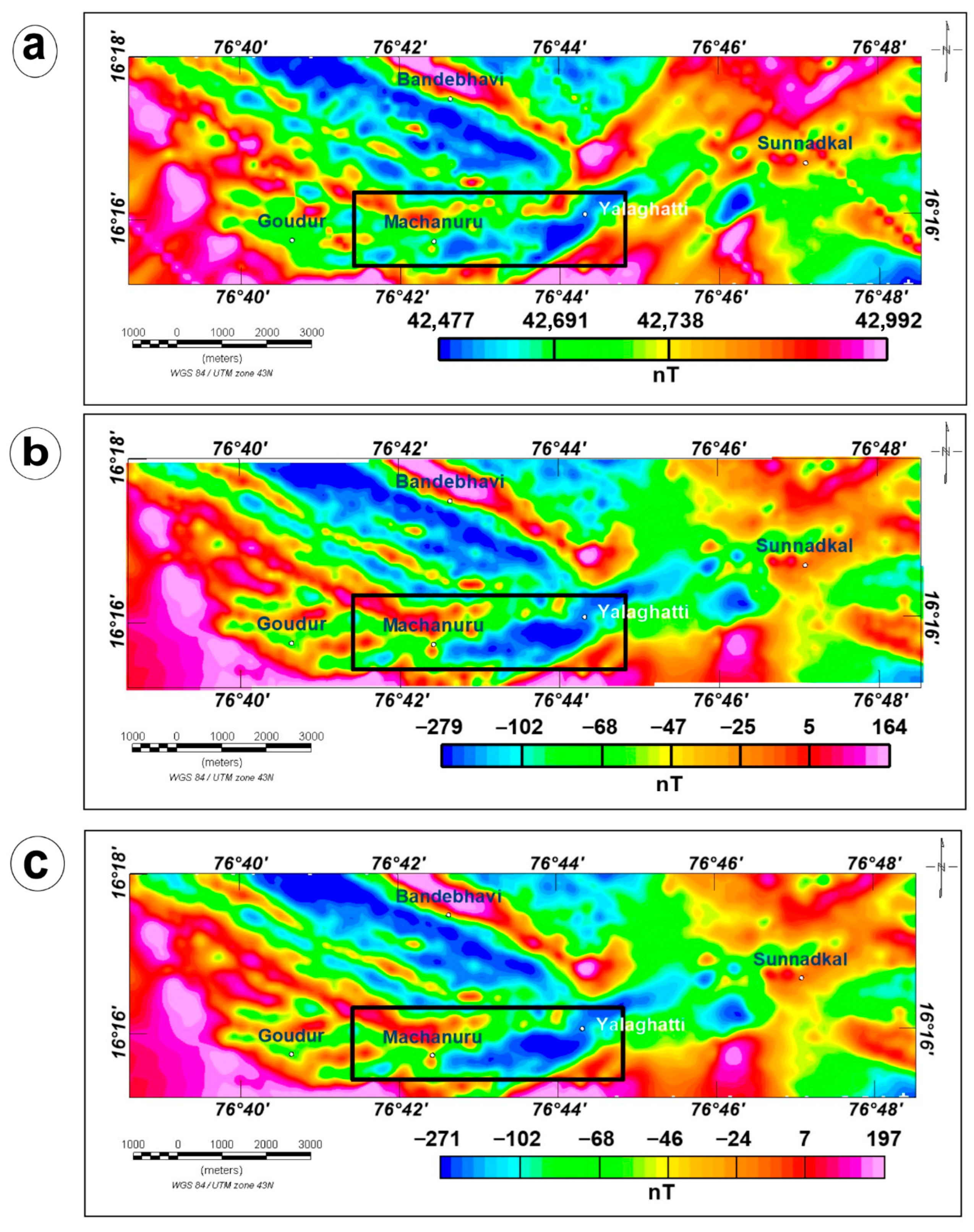
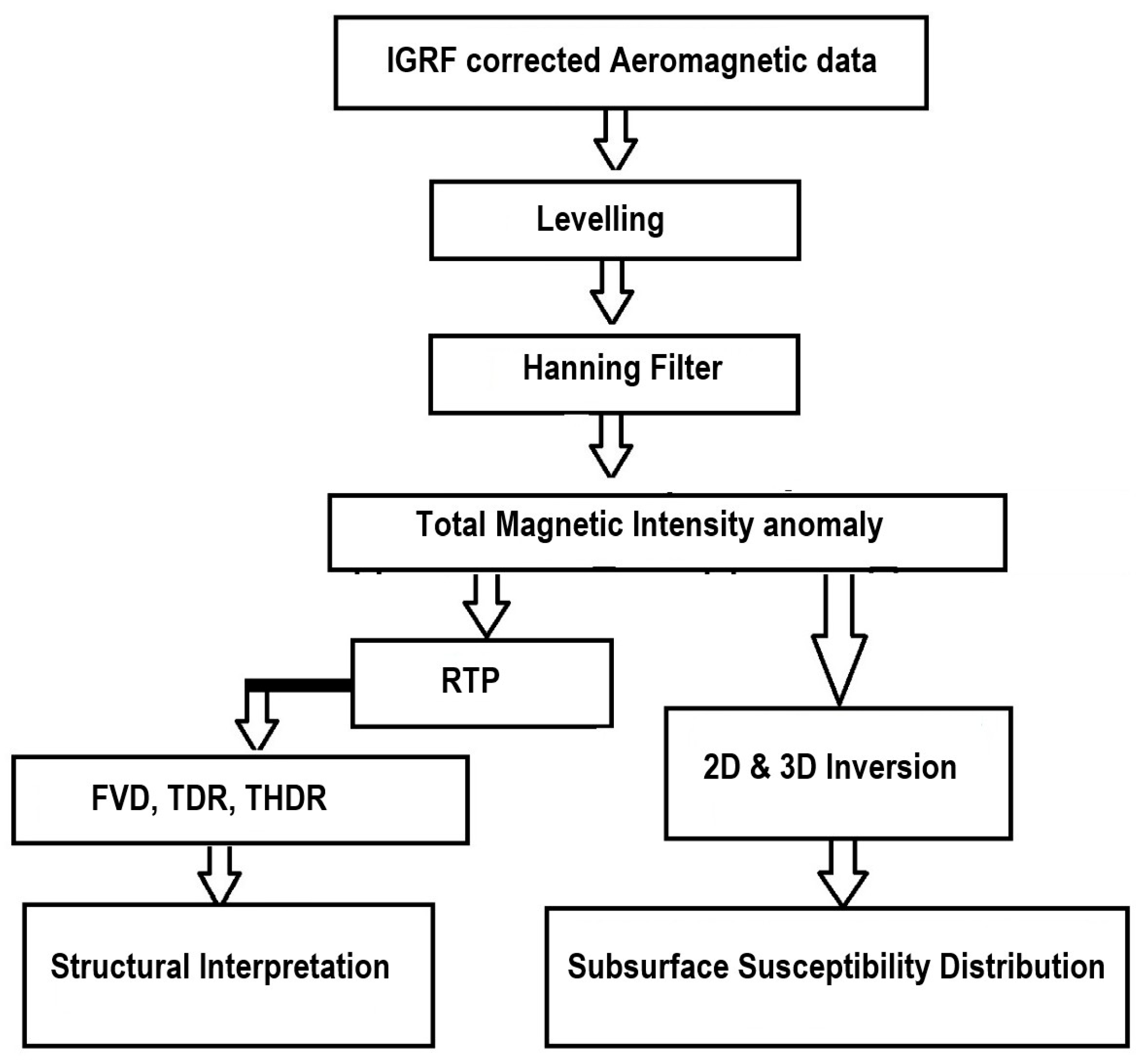
The workflow for the sequential methodology followed in this study is illustrated in Figure 2. The International Geomagnetic Reference Field (IGRF)-corrected aeromagnetic data sets were obtained from the National Geoscience Data repository [13]. The Geological Survey of India collected these high-resolution aeromagnetic data (Figure 3a). The survey was conducted in a northeast–southwest direction, with a traverse spacing of 300 m and a tie-line spacing of 3000 m. The data were acquired at a terrain clearance of 80 m above ground level (AGL). To enhance the reliability of our findings, we implemented advanced techniques, such as tie-line levelling and micro-levelling, to eliminate residual errors (Figure 3b), complemented by a Hanning filter to refine the data using Geosoft Oasis Montaj v.9.2 (Figure 3c).

Aeromagnetic data interpretation is a powerful approach for understanding subsurface geology, delineating magnetic source characteristics, and identifying structural controls that may govern mineralisation. To enhance the magnetic anomaly of the shallow structural features, several techniques have been employed, including RTP, FVD, TDR, and THDR. 2D magnetic inversion is attempted for a single profile which is perpendicular to the identified breccia zone. 3D magnetic inversion is also carried out to better constrain the source geometry for breccia zones. The theoretical basis and applications of these techniques are well documented in earlier studies (for example, [21,22,23,24,25,26,27,28]).

Dedicated analyses are carried out for the filtered aeromagnetic data for qualitative and quantitative interpretation (Figure 2). Analytical filters are applied to the output of the Hanning filter for refined data (Figure 3c) to infer the zone of target and associated magnetic structural features qualitatively. After that, the radially averaged power spectrum is estimated to infer the top of the magnetic horizon. Considering the initial depth parameters from the spectral method, 2D inversion is attempted for a single profile. 3D inversion is also carried out, considering the qualitative, spectral and 2D inversion results.

A concise overview of these methods and their relevance to mineral exploration is presented in the following section.

3. Results

3.1. Total Magnetic Intensity (TMI) Anomaly

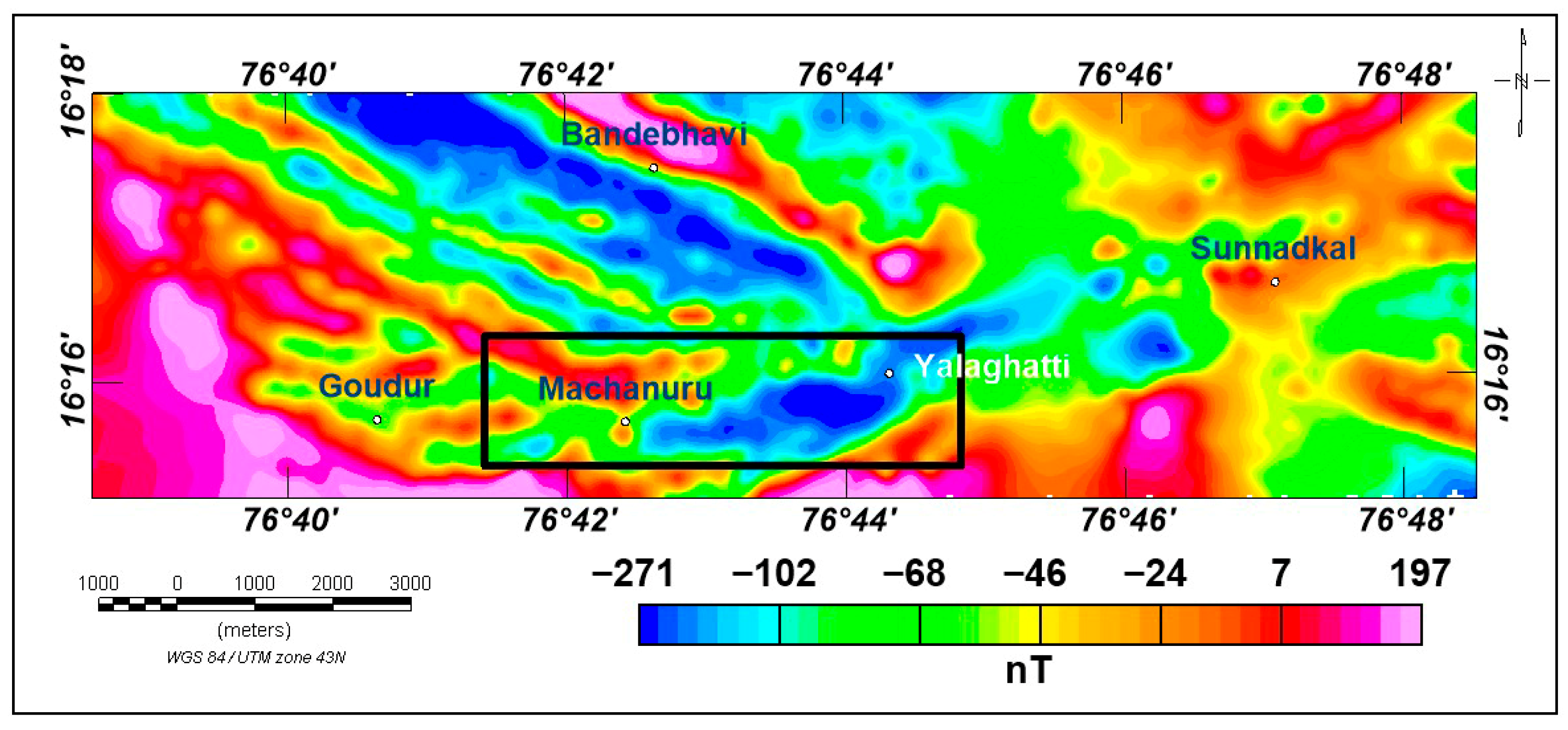
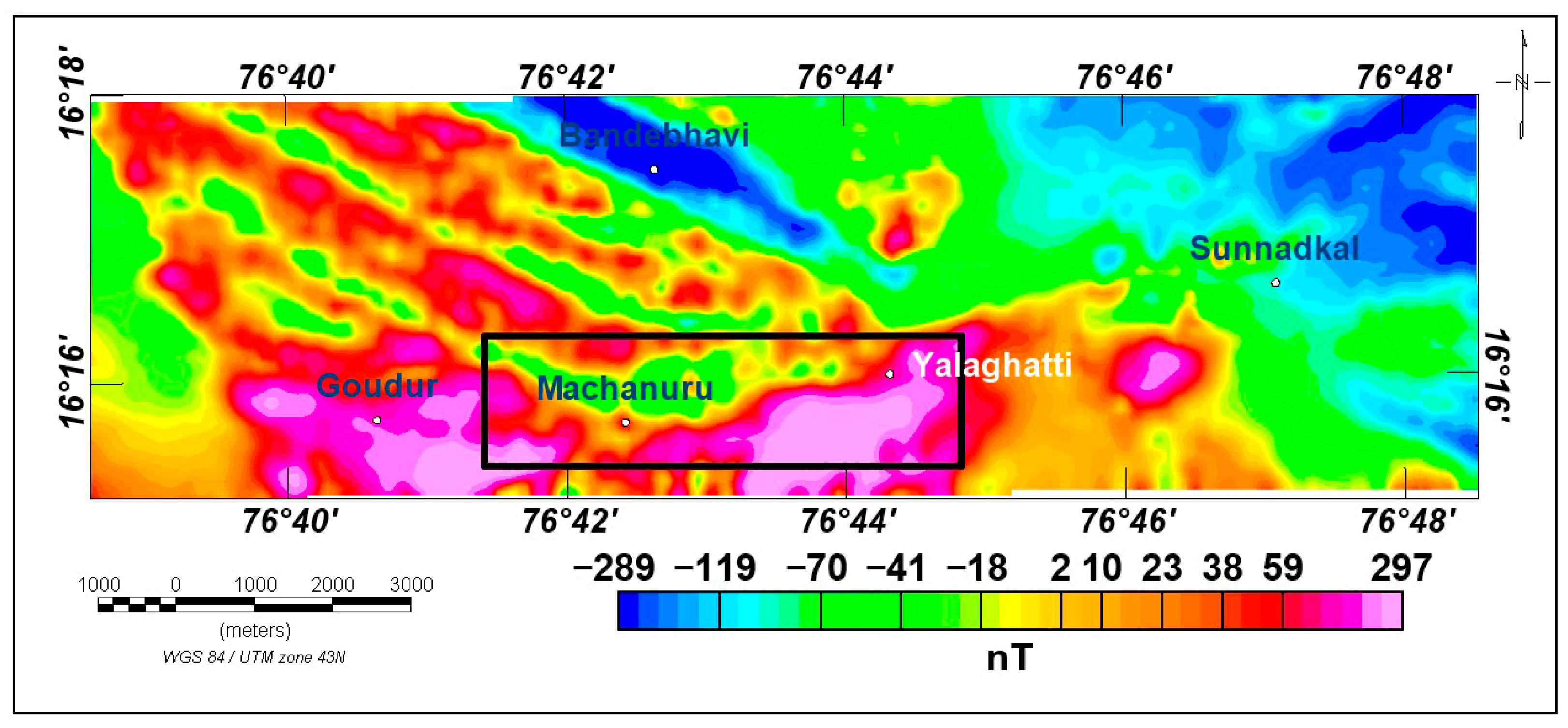
The corrected TMI anomaly image/map of the Machanur area and its surroundings is presented in Figure 4. Magnetic anomalies in the study area range from −270 to 195 nT with an amplitude of 460 nT. High intensity aeromagnetic anomalies (−50 nT to 195 nT) are observed near Goudur, Sunnadkal, Bandebhavi and south of Machanur from the TMI image/map. Low magnetic anomalies are observed at the east and north of the Machanur region near Yallaghati. The presence of high magnetic anomalies at Goudur, Bandebhavi corresponds to pillowed metabasalts with amphibolites, Granodiorite Gneiss, and pink granite. The associated magnetic high anomalies (−160 to 68 nT) in the Sunnadkal region are due to a suite of metabasalts, dolerites, quartzite veins, pink granite, and hornblende-biotite granite gneiss. The identified magnetic low at west and north of the Machanur region is indicative of the presence of pink and porphyritic granite. NW-SE, NE-SW, E-W, NNE-SSW, and ENE-WSW-trending magnetic lineations are observed throughout the area, indicating the structural fabric of the granite gneiss and its associated rocks.

An ENE-WSW trending magnetic low is mapped along the identified ductile to brittle shear zone associated with breccia. An amplitude of 300 nT is observed with a length of 7000 m and an average width of 700 m at the identified breccia zone (indicated as a black rectangle in the east of Machanur).

3.2. Reduction to the Pole (RTP) of the TMI Anomaly

The observed magnetic anomalies at any latitude appear as bipolar in nature except at magnetic poles. The observed magnetic anomalies’ deviations in the TMI map are due to this effect. Hence, to understand the true nature of the subsurface magnetic body’s characteristics, it is necessary to eliminate external geomagnetic influences. At this stage, the RTP filter is useful to reduce the asymmetrical effect on the natural magnetic field of the ore body. RTP is one of the analytical operators to understand the position of the sources independently of their magnetic inclination and declination. In this study, RTP is applied to TMI using the Geosoft Oasis Montaj software v.9.2 platform; it is an operator used in the frequency domain to transform asymmetrical anomalies to symmetrical anomalies [29,30,31,32]. In this transform, the geomagnetic field is assumed to be vertical and an assumed magnetic anomaly is directly over their causative source. Accordingly, see the following [33].

$$L\left(\theta \right)={\displaystyle \frac{1}{{\left[Sin\left(I\right)+iCos\left(I\right)Cos(D-\theta )\right]}^2}}$$

(1)

Here, θ represents the direction of the wavenumber vector;

I denotes the magnetic inclination;

D corresponds to the magnetic declination.

The present study area is located at low magnetic latitudes, with a magnetic inclination of 19.3° and a declination of −0.9°. It is observed from the RTP anomaly image/map (Figure 5) that the observed bipolar anomalies in the TMI (Figure 4) image are reoriented at Goudur, Machanur, Bandebhavi, and Sunnadkal regions. In general, as per the magnetic inclination at this region, the shape of observed anomalies would be low amplitude +ve magnetic high to high amplitude −ve magnetic low from south to north; the magnitude of the magnetic low is dominant. After applying the RTP filter, it is observed that the magnetic bipolar nature of the anomalies are omitted in the RTP map. The observed magnetic anomalies in the shear zone area (indicated by a black rectangle east of Machanur) appear as positive highs with an amplitude of ~300 nT after applying the RTP filter. Hence, the observed magnetic character indicates that the existing formations at the breccia zone might have remanence.

3.3. First Vertical Derivative (FVD) of TMI Anomaly

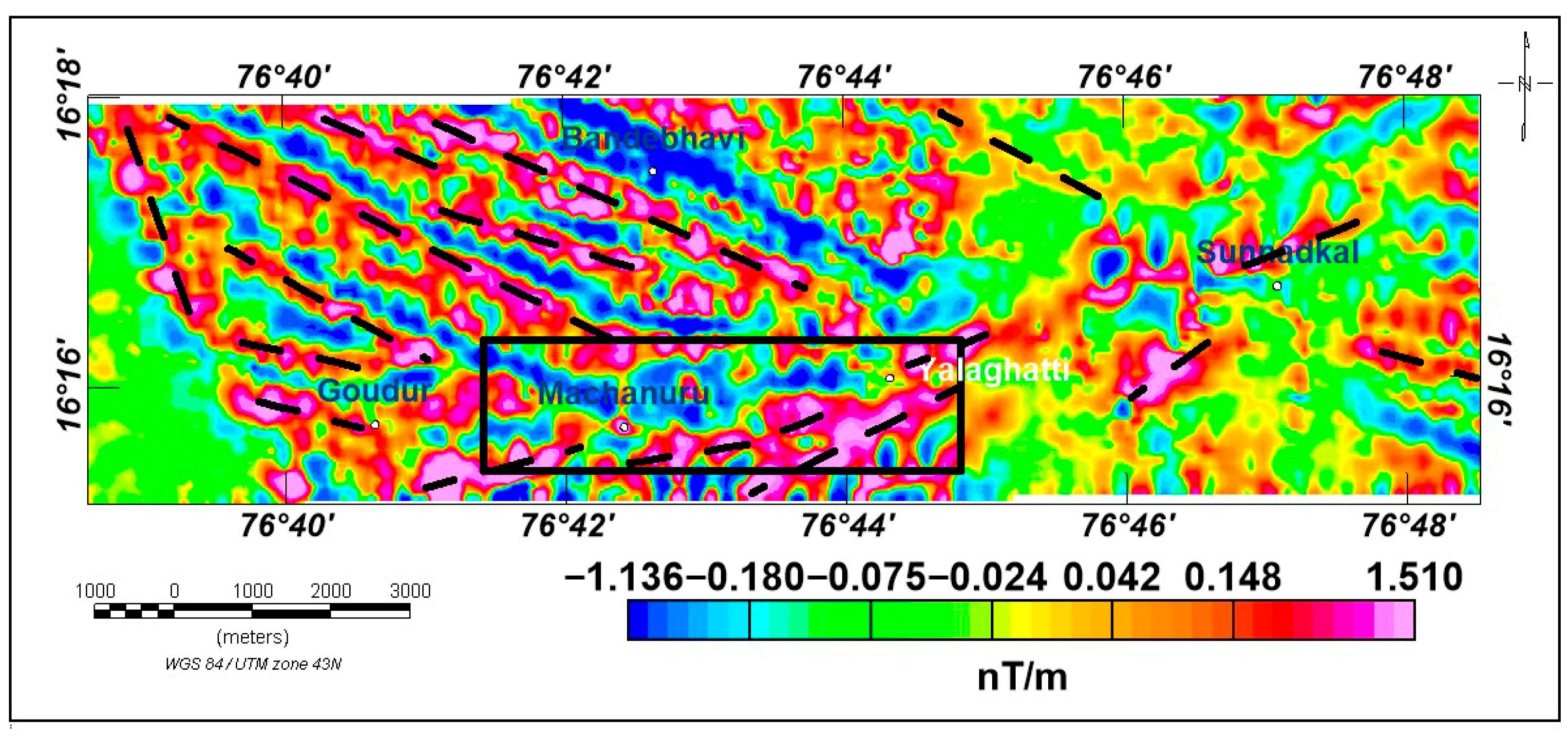
To understand the orientation of magnetic anomalies to infer the structural features’ characteristics, we have applied the FVD to the TMI anomaly (Figure 6).

$$FVD={\displaystyle \frac{\partial T}{\partial Z}}$$

(2)

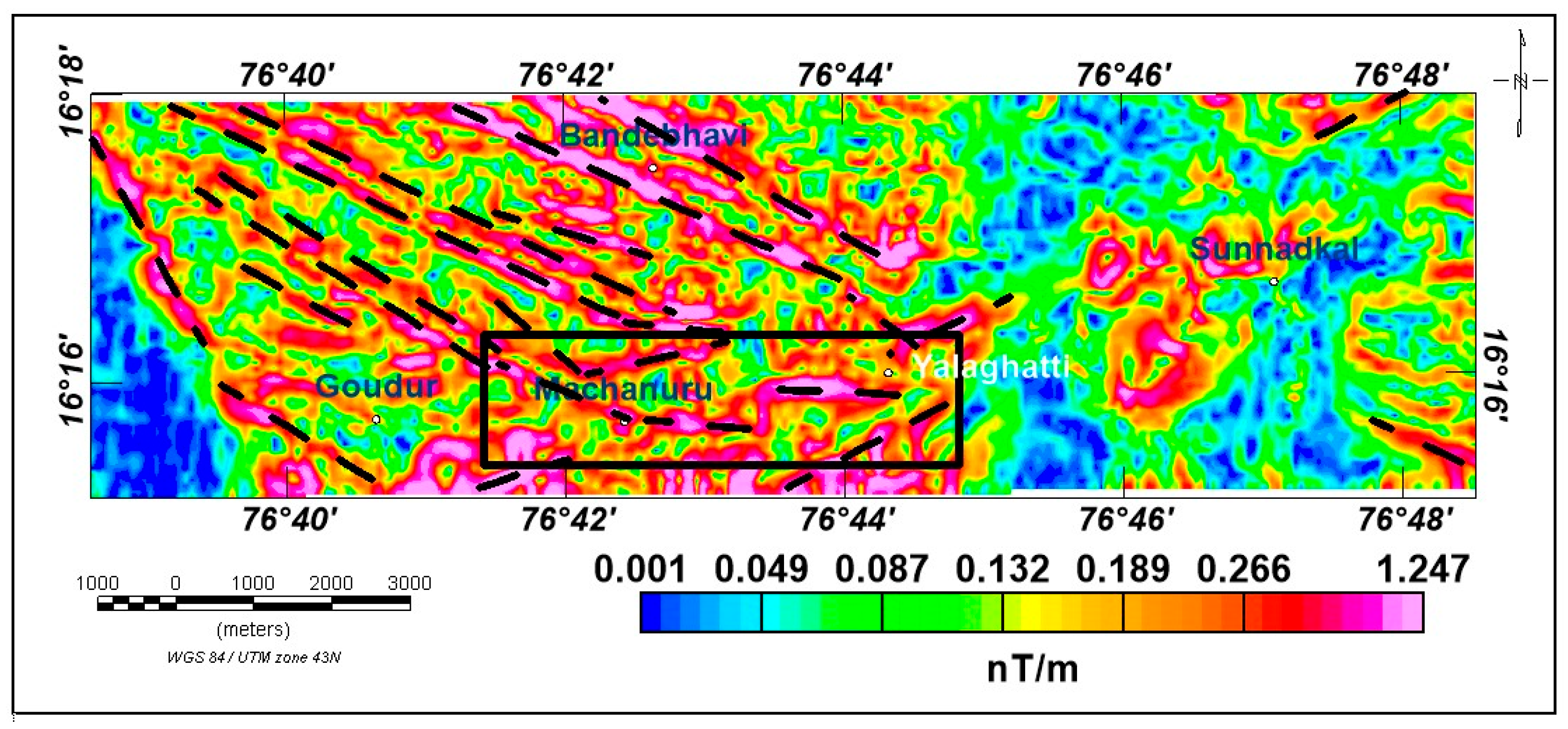
In the FVD map, SW-NE, NE-SW, E-W, and NNE-SSW magnetic lineations are observed. ENE-WSW magnetic high lineations characterise the targeted breccia zone. It is also observed that the discontinued magnetic lineations are observed in the breccia zones, which are perpendicular to the observed magnetic lineations in the north of Machanur.

This type of complex magnetic nature indicates that the extensive geological activities’ influence on the present study area may lead to the presence of a shear zone.

3.4. Tilt Angle Derivative (TDR)

The TDR is calculated as the arctangent of the ratio of the vertical and the total horizontal derivative of the magnetic field.

$$TDR={\tan }^{-1}\left({\displaystyle \frac{VDR}{THDR}}\right)$$

(3)

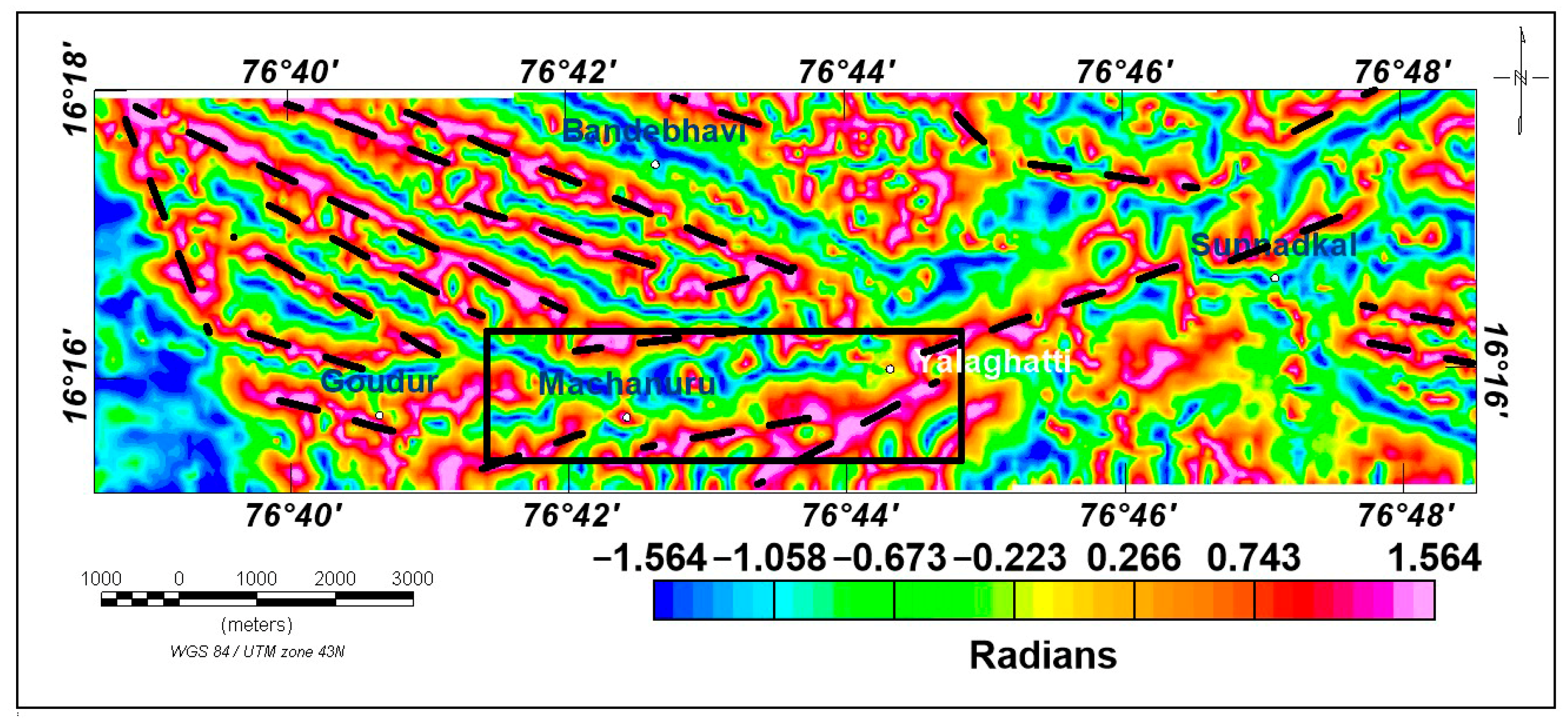
This method is well known for detecting geological boundaries and interpreting basement structures [26]. In this study, TDR also supports the identified magnetic lineaments from the FVD. Further, the extension of the ENE-WSW magnetic lineation at the identified breccia zone is noticed (Figure 7). The ENE-WSW trending magnetic lineation extending up to the Sunndakal region indicates the further extension of the breccia zone towards the west.

3.5. Total Horizontal Derivative (THDR)

The THDR is a widely used method for identifying the boundaries of magnetic sources [27]. One of the primary advantages of this technique is its reduced sensitivity to noise, as it relies exclusively on first-order derivatives in the horizontal direction [27]. THDR functions effectively as an edge-detection filter, making it proficient in outlining the edges of subsurface magnetic bodies. Mathematically, it can be expressed as follows:

$$THDR=\sqrt{{\left({\displaystyle \frac{\partial T}{\partial x}}\right)}^2+{\left({\displaystyle \frac{\partial T}{\partial y}}\right)}^2 }$$

(4)

Here, T represents the magnetic field, while ∂T/∂x and ∂T/∂y denote the two orthogonal components of the horizontal derivative of the magnetic field, respectively. The inferred magnetic lineations from FVD and TDR are also reflected in the THDR map; however, the extension of the breccia zone is restricted to Yalaghatti (Figure 8).

It is well-versed in the derivative images/maps (FVD, TDR, THDR) and magnetic lineaments observed in the X, Y, and Z directions, particularly SW-NE, NE-SW, E-W, and NNE-SSW. The identified breccia zone is characterised by an ENE-WSW magnetic high lineation and restricted to Yalaghatti, except in the TDR image.

3.6. Upward Continuation (UC) of TMI Anomaly

UC is a widely applied low-pass filtering method in aeromagnetic interpretation, in which the data are mathematically projected to a higher observation level, thereby increasing the effective distance between the sensor and the source bodies. This operation suppresses short wavelength components, including noise and near-surface variations, while emphasising longer wavelength signals associated with deeper geological structures, producing a smoother anomaly field [34,35].

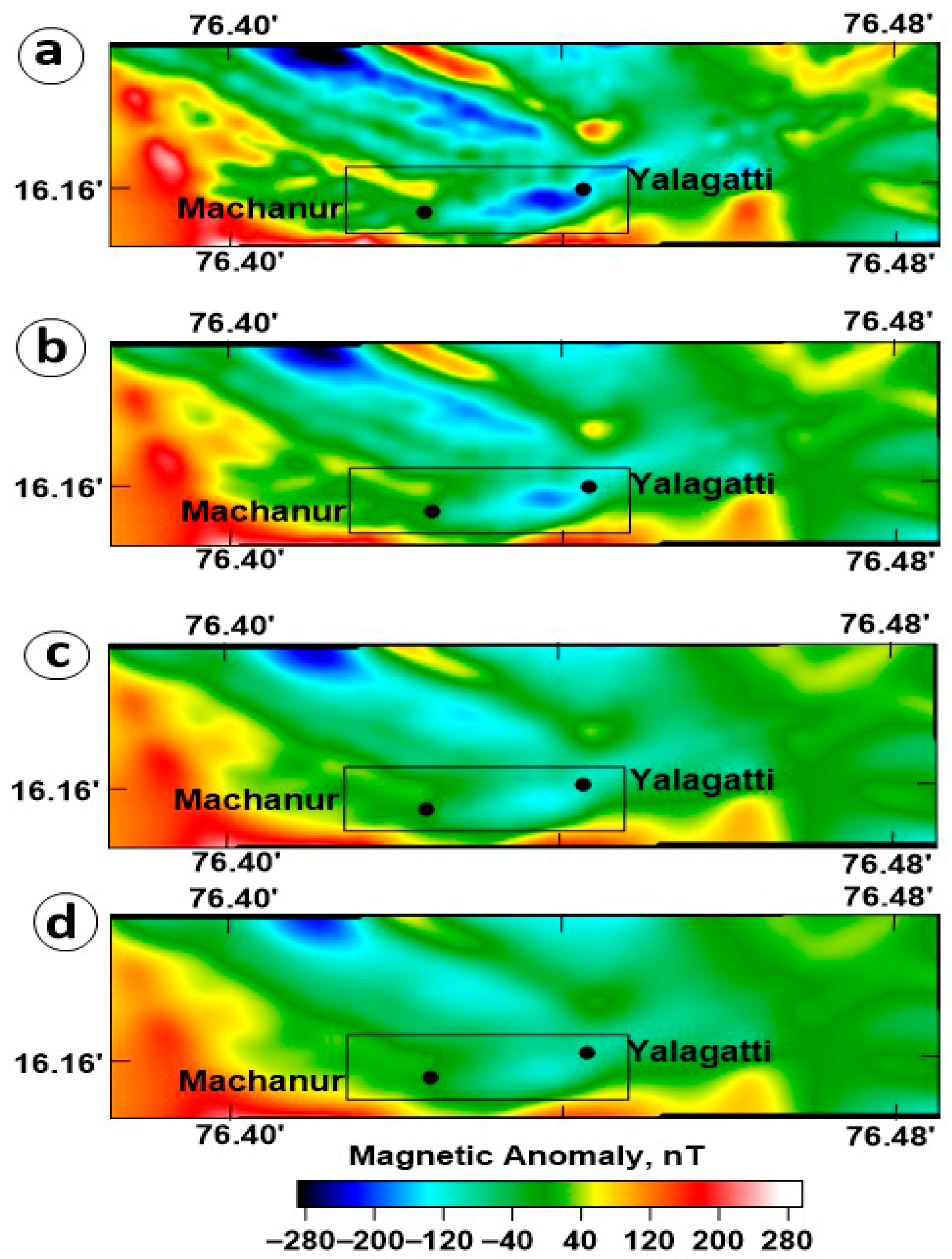
The UC is applied to the TMI anomaly to map the deeper sources; this technique enhances the anomalies originating from deeper sources while diminishing the effects of those caused by shallower sources. In this study, UC processes were performed at different heights from 100 m to 400 m with a height interval of 100 m (Figure 9a–d).

It is observed from upward continued TMI images at different altitudes that smaller, narrower, and thinner magnetic bodies tend to diminish progressively from shallow to deeper depths. The influences of larger magnetic bodies, which extend to greater depths, become more pronounced. It is well-versed from the Upward Continuation map; the signature of shear-zone-associated breccia is restricted to 400 m (Figure 9a–d). The UC of the study area up to a height of 100 m (Figure 9a) shows a prominent magnetic low at the identified shear zone, associated with breccia, with signatures of the Meta basalts, amphibolites, and pink granite. A cumulative magnetic signature is identified for NE-SW-oriented Dolarite, Meta basalts, Quartz, and Grano diorite gneiss geological formations (Figure 1b). The dominance of the magnetic low decreased in upward continuation image at 400 m height.

3.7. Semi-Quantitative Appraisal of Magnetic Data

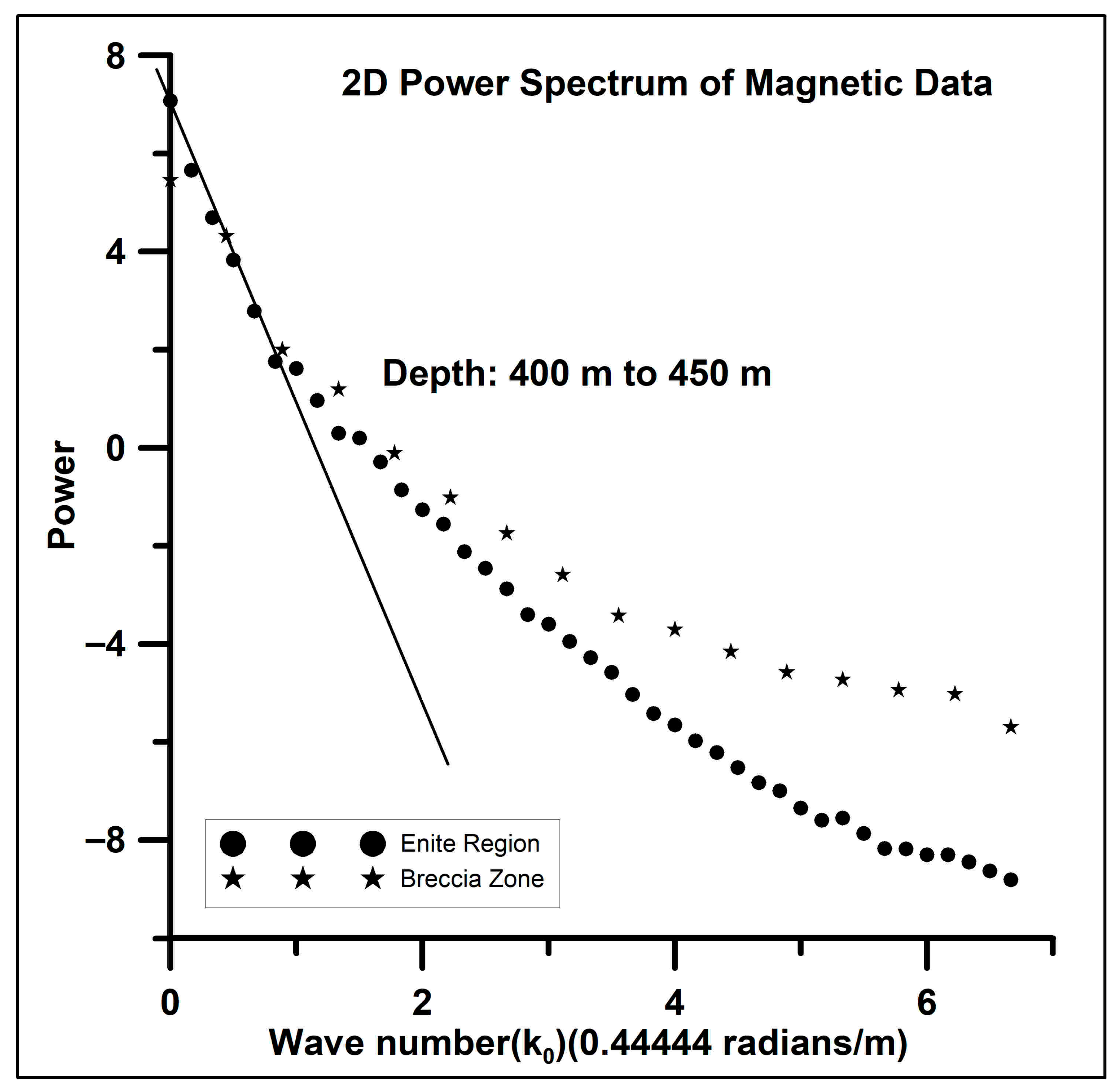
Long normalised radially averaged power spectrums [36,37] are calculated for the TMI anomaly (Figure 4) and TMI anomaly exclusively identified breccia zone (indicated by the black rectangle in Figure 4). The estimated depth from the identified magnetic slope from the two spectrums varies from 400 to 450 m (Figure 10). The estimated depth represents that a definite magnetic horizon is present between 400 m and 450 m from the surface. Hence, the thickness of the mineralised breccia zone may extend up to a depth of 450 m from the surface.

3.8. Two-Dimensional Model Studies

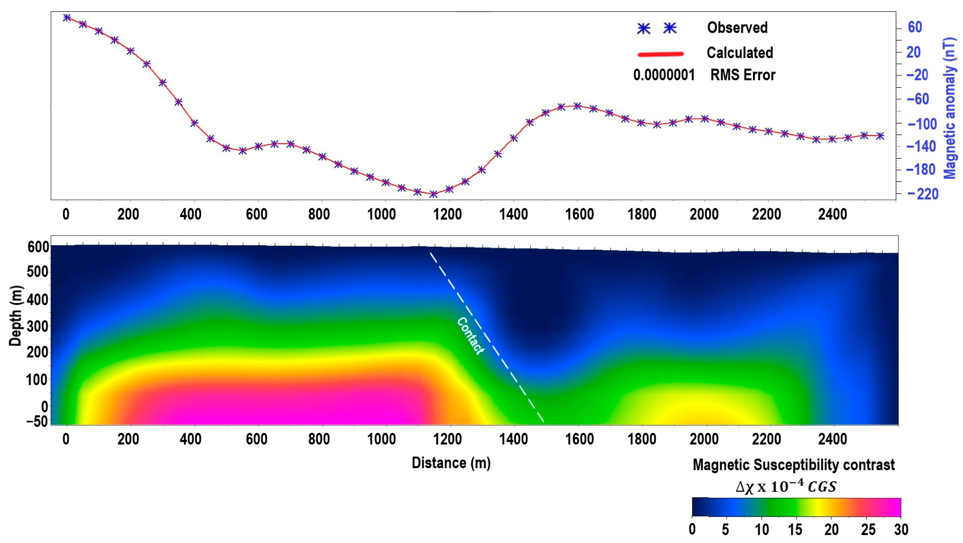
2D modelling is attempted for a single profile, which is perpendicular to the breccia zone. Profile AA¹ shows the location of the extracted magnetic profile (Figure 1b,c).

The 2D model is generated by using the Zond software package. 2D inversion for the aeromagnetic anomaly is attempted using the ZondGM2D v.5.1 inversion package, which is a user-friendly computer programme that utilises the various deconvolution and Newton’s regularisation methods, as follows:

$$\left(A^T{W}^{T}WA+\mathrm{\mu }{C}^{T}RC\right)\Delta m=A^T{W}^T\Delta f-\mu C^{T}RCm$$

(5)

where A denotes the Jacobian matrix, representing the partial derivatives of the observed data with respect to the model parameters. C corresponds to the smoothing operator, and W to the weighting matrix that accounts for relative measurement uncertainties. The vector m contains the model parameters, and μ is the regularisation coefficient. The term Δf denotes the residuals, defined as the difference between the observed and predicted data. R represents the focusing operator. It is inferred from the model studies that two distinguished layers are present below the anomaly zone, which are characterised by a low susceptibility layer underlain by a high susceptibility layer (Figure 11). The presence of low susceptibility at a shallow depth up to 400 m indicates the shearing/depletion of magnetic minerals in the layer at the breccia zone and also infers contact within the interpreted model, which is indicated by the magnetic variation within the granite. The interpreted magnetic high below the low magnetic anomaly is also due to pink phorphyritic granite. The interpreted magnetic model suggests the presence of the depleted magnetite content in the granitic formations.

3.9. 3D Modelling Studies

Magnetic anomaly interpretation has traditionally assumed that the causative sources are two-dimensional (2D), characterised by large strike lengths and uniform cross sections. Early approaches by [38,39] modelled irregular bodies by approximating their cross sections as multi-sided polygons and summing the magnetic contributions from each side. Later, ref. [40] refined these techniques for improved 2D modelling. However, such simplifications are rarely representative of natural geological bodies, which more commonly exhibit finite strike lengths (2.5D) [41,42] or fully three-dimensional geometries with variable cross sections [43]. Several formulations have been developed for 3D magnetic modelling, including prism-based solutions by [44,45], layer-based approaches by [46], and polygonal or polyhedral models by [47,48]. While earlier methods often relied on stacking simplified geometries and were sensitive to initial assumptions, rectangular prism models provide greater flexibility and are well-suited for automated inversion. Although 3D modelling is computationally intensive due to the need to process gridded data, modern computing capabilities make it both feasible and advantageous, as it yields more detailed insights into subsurface structures than 2D or 2.5D approaches. Consequently, the present study employs the UBC-Mag3D algorithm [49], which uses rectangular cell discretization to perform 3D inversion of magnetic data over the Machanur breccia zone.

Three-dimensional (3D) magnetic inversion is an effective technique for imaging variations in subsurface magnetic susceptibility and for validating the sources of magnetic anomalies. This study utilised the MAG3D inversion code [49] to analyse magnetic anomaly data and create a 3D distribution of the magnetic susceptibility of the selected area.

The UBC-GIF Mag3D inversion framework estimates a subsurface model that closely matches a reference physical property model while maintaining smooth changes between neighbouring cells [28]. The reference model can be based on the expected lithology, and the resulting solution represents the simplest model that fits both the geophysical data and available geological formation. In this study, no geological constraints were used. The inversion was carried out with standard parameter settings and a zero-reference model to obtain a physical property model that explains the observed geophysical data. These approaches have been commonly used in mineral exploration with UBC-GIF, v.5.0 software and have led to several successful applications [50,51,52,53,54,55].

The inversion process involves discretizing the subsurface into a 3D mesh of cells, which enables the reconstruction of magnetic susceptibility without prior assumptions about the geometry or physical properties of the sources [28]. For this analysis, a mesh cell size of 75 m × 75 m × 10 m (length × width × height) was utilised. Each observation point was assigned a 2% standard deviation with a minimum error of 5%, balancing model reliability with data sensitivity.

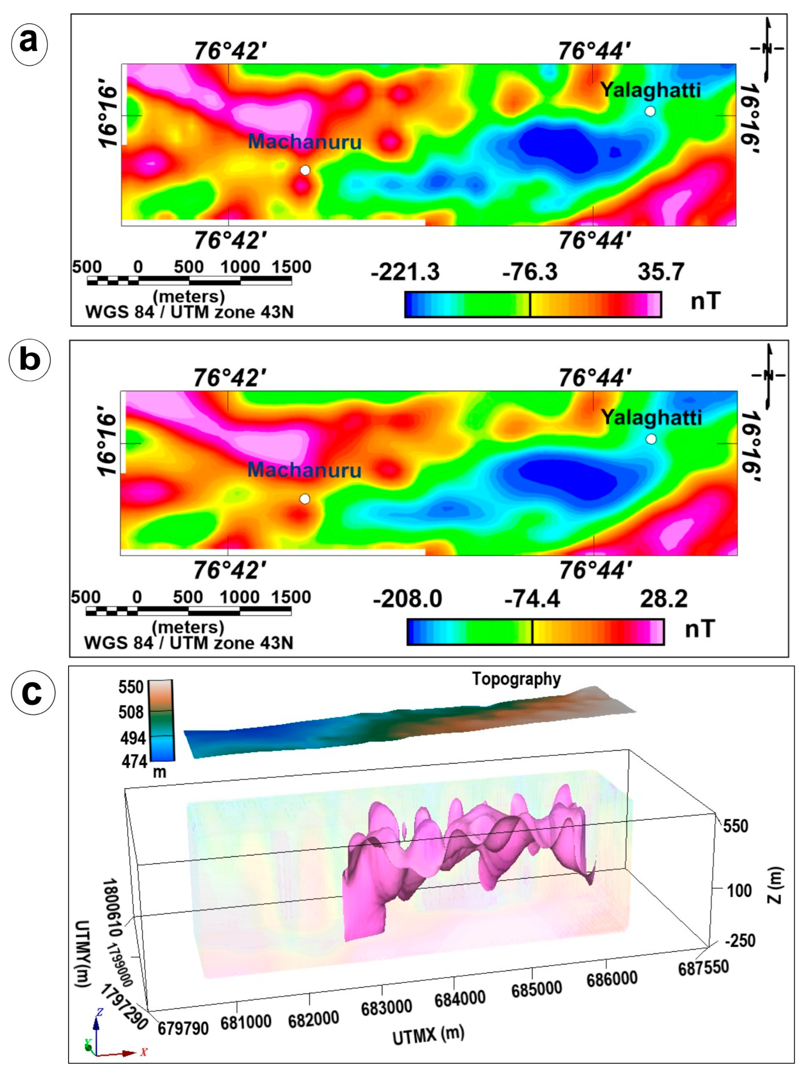
In the study area, the Earth’s total magnetic field measures approximately 42,300 nT, with an inclination of 19.3° and a declination of −0.9°. Figure 12a presents the TMI anomaly map used as input for the inversion. The inversion was performed using standard parameter values—chi = 0.02, αs = 0.0001, and αx = αy = αz = 1—which regulate model smoothness and stability.

The magnetic susceptibility of the base metal, used as a reference for interpreting mineralization, is approximately 0.005 SI units [56]. After an iterative approach, the calculated magnetic anomaly (Figure 12b) was obtained.

On the isosurface susceptibility map, an ENE-WSW blanket-shaped layer is observed along the identified breccia zone. The inferred depth of the layer is spread up to a depth of 400 m from the surface (Figure 12c).

4. Conclusions

The present study focuses on understanding the magnetic characteristics of the known breccia, which is associated with a shear zone with dimensions of 0.3 km by 5 km. The signatures of the aeromagnetic anomalies indicate the low magnetic nature of the breccia zone, with a 700 m-wide, 7 km-long magnetic anomaly. The qualitative analysis, using Reduction to Pole and Upward Continuation, indicates the extension of the zone to a depth of 400 m and has magnetic remanence. In the FVD, TDR, and THDR maps, the presence of SW-NE, NE-SW, E-W, and NNE-SSW magnetic lineaments and the breccia zone are characterised by an ENE-WSW magnetic high. The spectral and model studies are indicative that the average depth of this zone is 400 m. Corroboration among lithology, borehole, 2D and 3D magnetic anomaly interpretation results indicates the presence of a magnetic horizon up to an average depth of 400 m, which consists of sulphide mineralisation. The present study provides an additional magnetic parameter to characterise the breccia/shear zone in the terrain of granite gneisses in the Dharwar craton. The knowledge gained from the present analysis indicates an understanding of the concealed breccia zones in other parts of the region, which have been reported to be productive for mineralisation by previous researchers.

References

1. Allan, M.M.; Morrison, G.W.; Yardley, B.W.D. Physicochemical Evolution of a Porphyry-Breccia System: A Laser Ablation ICP-MS Study of Fluid Inclusions in the Mount Leyshon Au Deposit, Queensland, Australia. Econ. Geol. 2011, 106, 413–436. [Google Scholar] [CrossRef]
2. Anderson, E.D.; Atkinson, W.W.; Marsh, T.; Iriondo, A. Geology and geochemistry of the Mammoth breccia pipe, Copper Creek mining district, southeastern Arizona: Evidence for a magmatic–hydrothermal origin. Miner. Depos. 2009, 44, 151–170. [Google Scholar] [CrossRef]
3. Lin, B.; Tang, J.; Chen, Y.; Baker, M.; Song, Y.; Yang, H.; Wang, Q.; He, W.; Liu, Z. Geology and geochronology of Naruo large porphyry-breccia Cu deposit in the Duolong district, Tibet. Gondwana Res. 2019, 66, 168–182. [Google Scholar] [CrossRef]
4. Mondal, S.K.; Baidya, T.K.; Gururaja Rao, K.N.; Glascock, M.D. PGE and Ag mineralization in a breccia zone of the Precambrian Nuasahi Ultramafic-Mafic Complex, Orissa, India. Can. Mineral. 2001, 39, 979–996. [Google Scholar] [CrossRef]
5. Mondal, S.K.; Zhou, M.F. Enrichment of PGE through interaction of evolved boninitic magmas with early-formed cumulates in a gabbro–breccia zone of the Mesoarchean Nuasahi massif (eastern India). Miner. Depos. 2010, 45, 69–91. [Google Scholar] [CrossRef]
6. Sukanta, G.; Pradeep, K.U.; Saravanan, B.; Natarajan, V.; Verma, M.B. Two types of uranium mineralization in Gulcheru quartzite: Fracture-controlled in Ambakapalle area and litho-controlled in Tummalapalle area, Cuddapah Basin, Andhra Pradesh, India. China Geol. 2019, 2, 142–156. [Google Scholar] [CrossRef]
7. Bhattacharya, D.; Joshi, G.B.; Sharma, R. Uranium mineralization associated with felsic volcanism at Mohar, Shivpuri district, Madhya Pradesh. J. Geol. Soc. India 2011, 78, 57–62. [Google Scholar] [CrossRef]
8. Shukla, K.A.; Sharma, A. A brief review on breccia: Its contrasting origin and diagnostic signatures. Solid Earth Sci. 2018, 3, 50–59. [Google Scholar] [CrossRef]
9. Shukla, K.A.; Parasuram, B.; Basavaraja, K.; Mohanty, M. Iron oxide–copper–gold-type mineralization in Machanur area, Eastern Dharwar Craton, India. Curr. Sci. 2016, 111, 1853–1858. [Google Scholar]
10. Shukla, A.K.; Behera, P.; Basavaraja, K.; Praveen, M.N.; Korakoppa, M.M. Indication for Copper mineralization associated with Metabasalt in Gaudur area, Hutti-Maski Schist Belt, Raichur District, Karnataka. J. Appl. Geochem. 2019, 21, 438–442. [Google Scholar]
11. Shukla, K.A.; Dsilva, D.S.; Praveen, M.N. Granite-hosted Cu-Au Mineralization in the Machanur Deposit, Eastern Dharwar Craton. J. Geol. Soc. India 2023, 99, 291. [Google Scholar] [CrossRef]
12. Ramakrishnan, M.; Vaidyanadhan, R. Geology of India; Geological Society of India: Bangalore, India, 2008; Volume 1. [Google Scholar]
13. NGDR: National Geoscience Data Repository. Available online: https://geodataindia.gov.in (accessed on 4 October 2024).
14. Sultan, A.S.; Salah, A.M.; Fernando, M.S.; Ahmad, S.H. Geophysical exploration for gold and associated minerals, case study: Wadi El Beida area, South Eastern Desert, Egypt. J. Geophys. Eng. 2009, 6, 345–356. [Google Scholar] [CrossRef]
15. Gobashy, M.M.; Mekkawi, M.M.; Araffa, S.A.S.; Moahmed, M.E.E.; Mohamed, H.K. Magnetic Signature of Gold Deposits: Example from Um Garayat Region, South Eastern Desert, Egypt. Pure Appl. Geophys. 2023, 180, 1053–1080. [Google Scholar] [CrossRef]
16. Paasche, H.; Eberle, D.G. Rapid integration of large airborne geophysical data suites using a fuzzy partitioning cluster algorithm: A tool for geological mapping and mineral exploration targeting. J. Explor. Geophys. 2009, 40, 277–287. [Google Scholar] [CrossRef]
17. Hinze, W.J.; Von Frese, R.R.B.; Saad, A.H. Gravity and Magnetic Exploration Principles, Practices, and Applications; Cambridge University Press: New York, NY, USA, 2013; 515p. [Google Scholar] [CrossRef]
18. Cooper, G.R.J.; Cowan, D.R. 2008 Edge enhancement of potential-field data using normalized statistics. Geophysics 2008, 73, H1–H4. [Google Scholar] [CrossRef]
19. Fairhead, J.D. Advances in Gravity and Magnetic Processing and Interpretation; EAGE Publications: Houten, The Netherlands, 2015. [Google Scholar] [CrossRef]
20. Mishra, D.C.; Vijaya Kumar, V.; Rajasekhar, R.P. Analysis of airborne magnetic and gravity anomalies of peninsular shield, India, integrated with seismic and magnetotelluric results and gravity anomalies of Madagascar, Sri Lanka and East Antarctica. Gondwana Res. 2006, 10, 6–17. [Google Scholar] [CrossRef]
21. Archibald, N.; Gow, P.; Boschetti, F. Multiscale edge analysis of potential field data. Explor. Geophys. 1999, 30, 38–44. [Google Scholar] [CrossRef]
22. Nabighian, M.N.; Grauch, V.J.S.; Hansen, R.O.; LaFehr, T.R.; Li, Y.; Peirce, J.W.; Phillips, J.D.; Ruder, M.E. The historical development of the magnetic method in exploration. Geophysics 2005, 70, 33ND–61ND. [Google Scholar] [CrossRef]
23. Reeves, C. Aeromagnetic Surveys: Principles, Practice and Interpretation; Earth-Works: Washington, DC, USA, 2005; 155p. [Google Scholar]
24. Hood, P.J. Gradient measurements in aeromagnetic surveying. Geophysics 1965, 30, 891–902. [Google Scholar] [CrossRef]
25. Gunn, P.J.; Fitzgerald, D.; Yassi, N.; Dart, P. New algorithms for visually enhancing airborne geophysical data. Explor. Geophys. 1997, 28, 220–224. [Google Scholar] [CrossRef]
26. Miller, H.G.; Singh, V. Potential field tilt—A new concept for location of potential field sources. J. Appl. Geophys. 1994, 32, 213–217. [Google Scholar] [CrossRef]
27. Cordell, L.; Grauch, V.J.S. Mapping basement magnetisation zones from aeromagnetic data in the San Juan basin, New Mexico. In The Utility of Regional Gravity and Magnetic Anomaly Maps; Hinze, W.J., Ed.; SEG: Tulsa, OK, USA, 1985; pp. 181–197. [Google Scholar]
28. Li, Y.; Oldenburg, D.W. 3-D inversion of magnetic data. Geophysics 1996, 61, 394–408. [Google Scholar] [CrossRef]
29. Baranov, V. A New Method for Interpretation of Aeromagnetic Maps, Pseudo-Gravimetric Anomalies. Geophysics 1957, 22, 359–363. [Google Scholar] [CrossRef]
30. Baranov, V.; Naudy, H. Numerical calculation of the formula of reduction to the magnetic pole. Geophysics 1964, 29, 67–79. [Google Scholar] [CrossRef]
31. Blakely, R.J. Potential Theory in Gravity and Magnetic Applications; Cambridge University Press: Cambridge, UK, 1965. [Google Scholar]
32. Keating, P.; Zerbo, L. An improved technique for reduction to the pole at low latitudes. Geophysics 1996, 61, 131–137. [Google Scholar] [CrossRef]
33. Grant, F.S.; Dodds, J. MAGMAP FFT Processing System Development Notes; Paterson Grant and Watson Limited: Toronto, ON, Canada, 1972; 230p. [Google Scholar]
34. Jacobsen, B.H. Case for upward continuation as a standard separation filter for potential-field maps. Geophysics 1987, 52, 1138–1148. [Google Scholar] [CrossRef]
35. Betts, P.G.; Moore, D.; Aitken, A.; Blaikie, T.; Jessell, M.; Ailleres, L.; Armit, R.; McLean, M.; Munukutla, R.; Chukwu, C. Geology from aeromagnetic data. Earth-Sci. Rev. 2024, 258, 104958. [Google Scholar] [CrossRef]
36. Spector, A.; Bhattacharyya, B.K. Energy Density Spectrum and Autocorrelation Function of Anomalies Due to Simple Magnetic Models. Geophys. Prospect. 1966, 14, 242–272. [Google Scholar] [CrossRef]
37. Spector, A.; Grant, F.S. Statistical models for interpreting aeromagnetic data. Geophysics 1970, 35, 293–302. [Google Scholar] [CrossRef]
38. Talwani, M. Computation with the help of digital computer of magnetic anomalies caused by bodies of arbitrary shape. Geophysics 1965, 30, 797–817. [Google Scholar] [CrossRef]
39. Won, I.J.; Bevis, M. Computing the gravitational and magnetic anomalies due to a polygon. Algorithms and FORTRAN subroutines. Geophysics 1987, 52, 232–238. [Google Scholar] [CrossRef]
40. Murthy, I.V.R. Magnetic Anomalies of Two-Dimensional Bodies and Algorithm for Magnetic Inversion of Dykes and Basement Topographies. Proc. Indian Acad. Sci. 1990, 99, 549–579. [Google Scholar] [CrossRef]
41. Rasmussen, R.; Pederson, L.B. End corrections in potential field modelling. Geophys. Prospect. 1979, 27, 749–760. [Google Scholar] [CrossRef]
42. Cady, J.W. Calculation of gravity and magnetic anomalies of finite-length right polygonal prisms. Geophysics 1980, 45, 1507–1512. [Google Scholar] [CrossRef]
43. Murthy, I.V.R. Gravity and Magnetic Interpretation in Exploration Geophysics; Geological Society of India: Bangalore, India, 1998; 363p. [Google Scholar]
44. Bhattacharyya, B.K. Two-dimensional harmonic analysis as a tool for magnetic interpretation. Geophysics 1965, 30, 829–857. [Google Scholar] [CrossRef]
45. Sharma, P.V. Rapid computation of magnetic anomalies and demagnetization effects caused by bodies of arbitrary shape. Pure Appl. Geophys. 1966, 64, 89–109. [Google Scholar] [CrossRef]
46. Parker, R. The rapid calculation of potential anomalies. Geophys. J. R. Astron. Soc. 1973, 31, 447–455. [Google Scholar]
47. Plouff, D. Gravity and magnetic fields of polygonal prisms and application to magnetic terrain corrections. Geophysics 1976, 41, 727–741. [Google Scholar] [CrossRef]
48. Barnett, C.T. Theoretical modelling of the magnetic and gravitational fields of an arbitrarily shaped three-dimensional body. Geophysics 1976, 41, 1353–1364. [Google Scholar] [CrossRef]
49. UBC-GIF. MAG3D Inversion v.5.0: A Program Library for Forward Modelling and Inversion of Magnetic Data over 3D Structures; Geophysical Inversion Facility, Department of Earth and Ocean Sciences, the University of British Columbia: Vancouver, BC, Canada, 2013. [Google Scholar]
50. Watts, A. Exploring for nickel in the 90s, or ‘til depth us do part’. In Proceedings of Exploration 97: Fourth Decennial International Conference on Mineral Exploration; Gubins, A.G., Ed.; Prospectors and Developers Association of Canada: Toronto, ON, Canada, 1997; Volume 97, pp. 1003–1014. [Google Scholar]
51. Macdonald, J. The Role of Geosciences in Attracting Investment. In Proceedings of the World Mines Ministries Forum, Toronto, ON, Canada, 13–15 March 2002. [Google Scholar]
52. Hart, J.; Freeman, H. Geophysical responses of the Prominent Hill Fe-Cu-Au-U deposit. In Proceedings of the ASEG 16th Geophysical Conference & Exhibition, Adelaide, Australia, 16–19 February 2003. [Google Scholar]
53. Seshu, D.; Satish Kumar, K.; Sivasankar, P.; Kumar, P. Delineation of Concealed Banded Iron Formations (BIFs) below the Kurnool sediments in Palnadu Sub-basin, Macherla region, Cuddapah basin through 3D inversion of Aeromagnetic data. Geosystems Geoenviron. 2025, 4, 100357. [Google Scholar] [CrossRef]
54. Seshu, D.; Satish Kumar, K.; Pradeep Kumar, V.; Pranav, K.P.; Kumar, P. A note on aeromagnetic evidence of epigenetic Gold-Sulphide mineralisation in BIFs at Girar, Bundelkhand Craton, India. J. Geol. Soc. India 2025, 101, 1287–1289. [Google Scholar] [CrossRef] [PubMed]
55. Seshu, D.; Pradeep Kumar, V.; Rao, G.S.; Satyanarayana, H.V.S.; Kumar, P. Aeromagnetic analysis of the Shear zone of Ambaji granulite, NW India: Implications for base-metal mineralisation. Sci. Rep. 2026, 16, 12173. [Google Scholar] [CrossRef] [PubMed]
56. Hunt, C.P.; Mosowitz, B.M.; Banerjee, S.K. Magnetic properties of rocks and minerals. In Rock Physics and Phase Relations: A Handbook of Physical Constants, AGU Reference Shelf 3; Ahrens, T.J., Ed.; AGU: Washington, DC, USA, 1995; pp. 189–204. [Google Scholar]
Figure 1. (a) Regional geological map of Southern India (after [12]), (b) detailed geological map of the study area with selected profile AA1 for magnetic modelling (indicate white colour line) [13], (c) distribution of mineralisation within the breccia zone at Machanur (after [9]), and selected profile AA1 for magnetic modelling (indicate white and red colour lines), identified breccia zone indicated as a black rectangle in the east of Machanur.
Minerals 16 00581 g001
Figure 2. A schematic illustration of the workflow implemented for magnetic data.
Minerals 16 00581 g002
Figure 3. TMI image (a) after IGRF correction [13] (b) after levelling correction, and (c) after Hanning filter. The identified breccia zone is indicated as a black rectangle in the east of Machanur.
Minerals 16 00581 g003
Figure 4. TMI anomaly image/map of the study area; identified breccia zone is indicated as a black rectangle in the east of Machanur.
Minerals 16 00581 g004
Figure 5. RTP image/map of the study area; identified breccia zone is indicated by a black rectangle in the east of Machanur.
Minerals 16 00581 g005
Figure 6. First vertical derivative (FVD) image/map of the study area; identified breccia zone is characterised by an ENE-WSW magnetic high lineation. Identified breccia zone is indicated by a black rectangle in the east of Machanur. The black dotted lines indicate the identified magnetic lineaments.
Minerals 16 00581 g006
Figure 7. Tilt angle derivative (TDR) image/map of the study area; identified breccia zone is characterised by an ENE-WSW magnetic high lineation. Identified breccia zone is indicated by a black rectangle in the east of Machanur. The black dotted lines indicate the identified magnetic lineaments.
Minerals 16 00581 g007
Figure 8. Total horizontal derivative (THDR) image/map of the study area; identified breccia zone is characterised by a discontinued ENE-WSW magnetic high lineations. Identified breccia zone is indicated by a black rectangle in the east of Machanur. The black dotted lines indicate the identified magnetic lineaments.
Minerals 16 00581 g008
Figure 9. Upward Continuation height images of the study area at (a) 100 m, (b) 200 m, (c) 300 m and (d) 400 m. The dominance of the magnetic signature at the breccia zone (indicated as black rectangle box) at 100 m and 200 m height images compared to the 300 m and 400 m.
Minerals 16 00581 g009
Figure 10. Log-normalised average power spectrum for entire data (indicated by dotted symbol) and exclusively identified breccia zone (indicated by star symbol) shows that one straight line segment and estimated depth varies from 400 m to 450 m.
Minerals 16 00581 g010
Figure 11. 2D inversion model along the profile A–A1.
Minerals 16 00581 g011
Figure 12. 3D magnetic inversion model showing (a) what was observed, (b) predicted magnetic anomaly, and (c) distribution of isosurface susceptibility of 0.005 SI with topography of breccia zone (upper panel).
Minerals 16 00581 g012
Disclaimer/Publisher’s Note: The statements, opinions and data contained in all publications are solely those of the individual author(s) and contributor(s) and not of MDPI and/or the editor(s). MDPI and/or the editor(s) disclaim responsibility for any injury to people or property resulting from any ideas, methods, instructions or products referred to in the content.