A Multi-Proxy Framework for Predicting Ore Grindability: Insights from Geomechanical and Hyperspectral Measurements

Abstract

Accurate characterization of ore grindability is essential for optimizing mill throughput, reducing energy consumption, and predicting mill performance under varying ore conditions. However, the standard Bond work index (BWI) test remains time-consuming, costly, and requires a large amount of sample. This study evaluates the effectiveness of several rapid, low-cost alternatives, Leeb rebound hardness (LRH), Cerchar abrasivity Index (CAI), portable X-ray fluorescence (pXRF), and hyperspectral imaging (HSI), as proxies for grindability in gold-bearing ores. Sixty-two hand-size rock samples collected from two adjacent Canadian open-pit mines were analyzed using these techniques and subsequently grouped into ten ore groups for BWI testing. LRH and CAI effectively differentiated moderate (<15 kWh/t) from hard (>15 kWh/t) grindability classes, while geochemical features and HSI-based mineralogical attributes also showed strong predictive capability. HSI, in particular, provided non-destructive, spatially continuous data that are advantageous for complex geology and large-scale operational deployment. A conceptual workflow integrating HSI with complementary field measurements is proposed to support comminution planning and optimization, enabling more responsive and timely decision-making. While BWI testing remains necessary for circuit design, the results highlight the value of combining rapid proxy measurements with advanced analytics to enhance geometallurgical modelling, reduce operational risk, and improve overall mine-to-mill performance.

1. Introduction

Strategic mine planning is crucial for maximizing the economic potential of a mining operation. It primarily focuses on two key aspects: optimizing the ultimate pit limit and the production schedule for the life of the mine (LOM), which considerably depends on the spatial variability of the ore deposit [1]. The term variability refers to fluctuations observed in successive values of the deposit, such as ore grade. If such variability is not spatially quantified, it heightens project risks and increases the potential for revenue loss, particularly through a reduced net present value [2].

Geometallurgy represents an interdisciplinary field that integrates geology, mining, mineral processing, geotechnical engineering, metallurgy, mineral economics, and geoenvironmental parameters, with the primary aim of maximizing project value, reducing technical risks, enhancing operational resilience, and optimizing the use of mining resources [2]. It aims to forecast the occurrence of disruptive events and enhance the operation’s capability to respond to and recover from such events. A sustained period of extreme hard ore feed to the comminution process could be a clear example of such a disruptive situation, resulting in increased processing time and energy consumption per unit of material processed, and increasing the need for equipment maintenance. This situation could be effectively addressed by a better prioritizing and blending strategy.

Geometallurgical variables are rock attributes that influence resource value, which can be classified into two categories: primary and response variables [3]. Primary variables reflect intrinsic rock properties, measured directly to predict metallurgical responses. Examples include ore hardness and ore grade. Conversely, response variables refer to the rock’s characteristics that indicate how it responds to metallurgical processes, such as comminution and flotation. Key metallurgical response variables include recovery, throughput rate, concentrate grade, grindability, and liberation [4].

Comminution serves as a crucial means of liberating valuable minerals from the gangue. The process involves reducing the particle size of the mined ore, making the subsequent separation and extraction stages more efficient [5]. Its performance significantly affects planned production and mill throughput, with significant economic consequences. Comminution consumes a substantial portion of the energy used in mine-to-mill operations. On a local mining scale, it has been estimated that comminution accounts for up to 50% of total energy consumption, while on the global scale, comminution energy consumption is approximately 2%–3% of total worldwide energy [6,7,8]. Therefore, understanding and optimizing the comminution process can improve the economic and environmental sustainability of the mine-to-mill operations.

A key challenge in optimizing comminution is accurately determining the energy required to process different ore types throughout the LOM. One of the widely used comminution tests is the Bond work index (BWI), which measures the energy required for grinding ore. The Standard BWI testing procedure [9] is time-consuming, labor-intensive, and requires a significant mass of rock samples [10,11,12]. It involves grinding a significant mass of rock sample, usually around seven to ten kilograms (kg), which can take up to 10 h to complete [13]. These conditions make the BWI testing method impractical for routine use, especially in the fast-paced mining environment [14], resulting in insufficient characterization of the grindability variability, which is essential for reducing uncertainty in the subsequent processing performance.

Numerous attempts have been made to address the challenges of performing the BWI testing method, which can be summarized into two main categories. On the one hand, researchers have sought to simplify the BWI testing procedure by reducing the required sample mass and eliminating unnecessary steps, thereby making it more practical and easier [11,15,16,17,18,19,20]. On the other hand, a wide variety of research has focused on developing proxies to characterize the grinding behavior of ore by investigating the relationship between the results of the BWI test and other physico-mechanical properties of rocks, which are generally measured for rock engineering purposes at the mine site.

Deniz and Ozdag [8] investigated the relationship between BWI and the dynamic elastic parameters of different sedimentary and volcanic rocks. Ozkahraman [21] explored the potential application of the brittleness test in predicting BWI values. The results showed that the BWI values can be determined based on the brittleness values of the material, a conclusion confirmed later by Swain and Rao [22]. Montoya et al. [23] developed models to classify the comminution breakage parameters in a large-scale geometallurgical study by integrating Leeb rebound hardness (LRH) and quantitative mineralogy data. Gent et al. [24] found a strong relationship between Vickers hardness and energy consumption during comminution of brittle minerals. Haffez [25] examined the mechanical properties of various ores, including bauxite, kaolinite, granodiorite, magnetite, granite, feldspar, and quartz, in relation to the BWI. The results indicated that the BWI positively correlates with the modulus of elasticity, Rockwell hardness, and uniaxial compressive strength. Conversely, abrasion exhibited a negative correlation with BWI. Harbort et al. [26] conducted a study and found a correlation between the results of the Drop Weight test (Axb) and BWI using data from different rock types.

Hunt et al. [27] attempted to predict the comminution parameters, including BWI values, using available field data, such as mineralogical and alteration data. The results indicated that the comminution parameters can be predicted using the mineralogical and alteration data. They also noted that the estimated comminution parameters could be incorporated into the mine database, providing geometallurgical inputs for spatial modeling, mine planning, and optimization. Chandar et al. [28] conducted a systematic investigation to develop predictive models for BWI using simple field-measurable rock characteristics, such as density, strength, and rebound hardness value. They performed the tests on different rock types, such as Basalt, Slate, and Granite, and found good correlations between the mentioned rock characteristics and BWI.

Bhuiyan et al. [14] conducted a practical geometallurgical testing program to predict BWI using rock characterization tests. Physical, mechanical, mineralogical, geochemical, and textural properties of rocks were studied. The results of the statistical analyses showed that the geochemical properties strongly correlate with BWI and that the geochemical data can be used to classify the samples into different geometallurgical domains. van Duijvenbode et al. [29] presented an agglomerative hierarchical clustering approach to categorize the typical grindability of various rock types in a gold mine using geochemical and hyperspectral data in visible-near infrared (VNIR) and short-wave infrared (SWIR). LRH and BWI were performed on the rock samples to assess their grindability. The obtained classes, from geochemical and hyperspectral data, were used to define the geochemical domains, and the relationship between these domains and grindability was studied. They found that identified geochemical domains could assist in interpreting different processing proxies such as LRH and BWI tests.

Most recently, Both and Dimitrakopoulos [30] presented a novel approach to predict ball mill throughput in mining complexes by using readily available production data, penetration rates from measurement while drilling (MWD), and then integrating these predictions into short-term stochastic mine production scheduling. The primary motivation behind their research lies in the observation that conventional geometallurgical throughput prediction models rely on limited hardness data and often ignore the non-additive characteristics of hardness during the processes of upscaling and blending, resulting in inaccurate predictions and inefficient production schedules.

The primary purpose of this study is to investigate and compare the possible applications of several geochemical and geomechanical testing methods, including portable X-ray fluorescence (pXRF), LRH, Cerchar abrasivity index (CAI), and hyperspectral imaging (HSI) technique, in characterizing grindability behaviors of rocks during the comminution process. Compared with the BWI procedure, the mentioned testing methods are less resource-intensive and more time-efficient. They could be used to better understand the variability in comminution behavior and, ultimately, optimize comminution and subsequent processes. To the authors’ knowledge, no studies have investigated the relationship between BWI and the mentioned geomechanical, spectral, and geochemical testing methods and compared their performance, practicality, and data resolution. It is important to note that these approaches are not intended to replace BWI tests. A sufficient number of BWI measurements remains necessary for accurate geometallurgical characterization and proper comminution and processing design. However, the geomechanical, spectral, and geochemical proxies evaluated in this study can help capture spatial variability in ore grindability across the mine. By providing rapid, complementary information, these proxies can support more informed ore prioritization, blending, and processing decisions, thereby potentially avoiding processing and mill throughput bottlenecks by not feeding hard ore for prolonged periods. A brief description of the mentioned geochemical, spectral and geomechanical testing methods is provided below.

X-ray fluorescence (XRF) is a widely used method for determining the surface and bulk concentrations of chemical elements, which can be efficiently achieved with a pXRF analyzer. The pXRF analyzer enables rapid multi-element geochemical analysis of rock samples, making it a practical tool for geochemical pattern recognition [31]. Moreover, as a fast, non-destructive technique capable of simultaneously analyzing multiple elements in both unprepared and lab-prepared solid samples, pXRF serves as a time- and cost-efficient alternative to the more complex and expensive standard laboratory procedures like Inductively Coupled Plasma Atomic Emission Spectroscopy (ICP-AES) and Inductively Coupled Plasma Mass Spectrometry (ICP-MS) [32,33,34].

The LRH test is a portable, rapid, and non-intrusive method initially designed for assessing the hardness of metallic materials [35]. The rebound hardness value is calculated as a function of the ratio of the rebound velocity of an impact body to its impact velocity, which follows the principle of energy measurement. While the impact velocity is always constant, the rebound velocity is a function of the surface properties of rocks, and the harder the tested rock, the higher the Leeb rebound hardness value [36]. Compared with other rebound hardness testing methods, the LRH has a lower impact energy, broadening the LRH test applications. This is important since measuring the rebound hardness of weathered and weak rocks is always challenging using other hardness tests [37].

On the other hand, the CAI test is widely used to assess rock abrasivity and estimate wear on mechanical tools interacting with rocks. CAI testing is a rapid, laboratory-based index test that evaluates rock resistance to scratch and abrasiveness using prepared rock fragments of specified size. The test requires minimal sample preparation and provides a relative measure of rock hardness with good repeatability, making it suitable for comparative hardness assessment rather than absolute strength determination. CAI was initially developed for coal mining applications, this test has progressively been adopted in other geoengineering areas, including hard rock mining and tunneling [38,39,40]. The term abrasion refers to the wearing or tearing away of particles from a solid surface. This leads to the displacement or loss of material from the surface, resulting in wear, particularly on tools [41].

HSI is a powerful technology that combines spectroscopy with imaging capabilities. It enables gathering detailed information about the composition and characteristics of objects. It involves using an imaging spectrometer, also called a hyperspectral camera, to collect spectral information. A hyperspectral camera captures the reflected light from a scene. It provides a two-dimensional image of the scene while simultaneously recording the spectral information of each pixel in the image [42]. A hyperspectral image is a spectral data cube composed of N spatial samples (pixels), where each pixel is represented by an M-dimensional spectral vector corresponding to M spectral bands. The hyperspectral sensor uses numerous narrow electromagnetic wave bands to obtain relevant information from objects. As a fast, non-destructive, high spectral resolution, hyperspectral imaging can be employed in remote areas to quickly gather extensive data, enabling engineers to understand material properties throughout the entire mine-to-mill process comprehensively. Hyperspectral remote sensing has recently expanded into geoengineering applications, including the characterization of rocks’ physical, geochemical, and mechanical properties [29,43,44,45,46,47,48,49,50,51,52,53].

2. Materials and Methods

2.1. Data Collection

The dataset consists of 62 hand-picked specimens, systematically collected by the mine’s ore control team along the dig lines at two adjacent open-pit gold mines in the northeast of Canada. The samples represent sedimentary, ultramafic, and intrusive rock types with varying degrees of alteration. All rocks were taken directly from freshly blasted muck piles, ensuring that the exposed surfaces were not affected by long-term weathering or oxidation. This sampling approach aligns with the operational objective of the study to evaluate measurement techniques under conditions that closely reflect real mining environments. The main minerals identified in these rock samples include Quartz, Biotite, Muscovite, Chlorite, Dolomite, Calcite, Pyrite, Talc, Magnetite, Hornblende, Albite, and Potassium Feldspar [31].

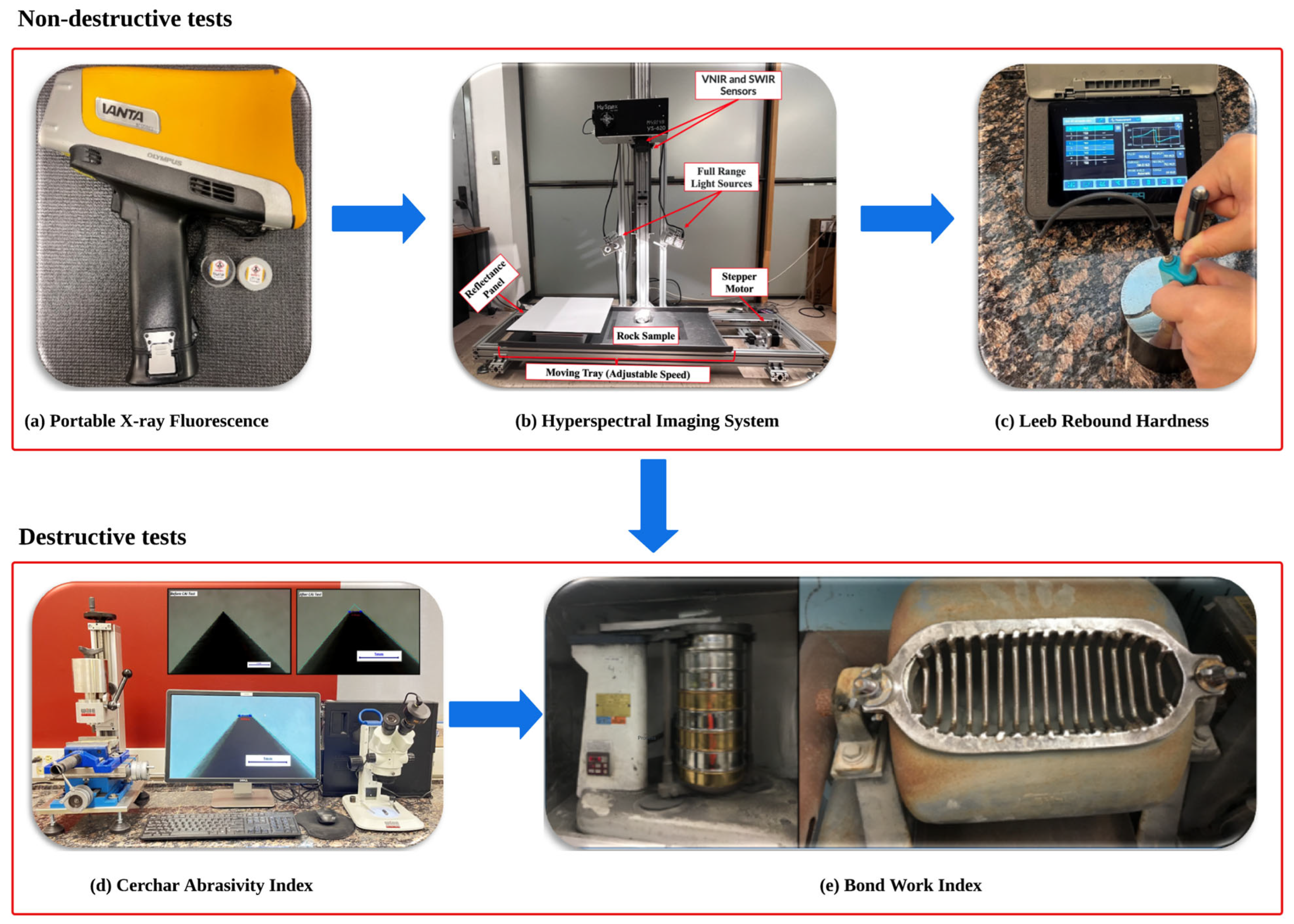
The data collection process involved several steps. Initially, a pXRF device was utilized to measure the surface concentration of chemical elements. Next, the collected rock samples were scanned using a hyperspectral imaging system. In the third step, the LRH test was conducted to determine the hardness of the rock samples. Afterward, the abrasivity was measured using the CAI test. Finally, the samples were mixed to form 10 ore groups, and the BWI test was performed on the ore groups to measure the required energy for grinding them in the comminution process. Figure 1 illustrates the different steps of the data collection stages, each explained in detail in what follows.

The measurement of surface chemical element concentrations was conducted using a 3-beam Olympus Vanta device (Olympus Corporation, Tokyo, Japan) specifically designed for mining and geological engineering applications (Figure 1a). To preserve the realism of field conditions, the samples were not polished, cut, or pulverized; all measurements were performed on the fractured rock surfaces, consistent with how pXRF is applied operationally. To ensure representative measurements, five readings were taken at different points on the surface of each rock sample and averaged. The spacing between measurement points was carefully considered to cover the entire testing surface. Each beam’s measuring time was set to the device’s maximum allowable duration to obtain the most robust results. The device was mounted on a mechanical holder for safety and to maintain constant contact with the rock sample during testing. The surface concentrations of elements, including Ag, Al, As, Ba, Ca, Cd, Ce, Co, Cr, Cu, Fe, Hg, K, LE, La, Mg, Mn, Mo, Nb, Nd, Ni, P, Pb, Pr, Rb, S, Sb, Si, Sn, Sr, Th, Ti, U, V, W, Y, Zn, and Zr, were determined in parts per million (ppm). To ensure the accuracy of these measurements, certified reference material (CRM) SRM2711a and a Silica blank sample were utilized at the beginning of each testing session. Eighteen measurements were taken from both SRM2711a and the Silica blank to evaluate the precision and bias of the instrument. The processing of pXRF data is discussed in Section 2.2.

The rock samples were scanned in the second step using the HySpex Mjolnir VS-620 (Neo, Oslo, Norway) hyperspectral imaging system, which operates across the VNIR and SWIR spectral ranges. The technical characteristics of the sensors and the illumination system are summarized in

Table 1. Technical characteristics of the HySpex Mjolnir VS-620 system.

Component	Spectral Range (nm)	Spatial Pixels	Spectral Channels	Average Bandwidth (nm)
VNIR sensor	450–900	1240	200	3.0
SWIR sensor	900–2500	620	300	5.1
Light source	400–2500	–	–	–

.

The scanning process involved adjusting the integration time and using a spectral reference target (reflectance panel in Figure 1b) to convert radiance to reflectance [54]. Variations in rock types and mineralogy on the surface of rock samples could result in different albedo observations during lab scanning. Two diffuse reflectance panels with predetermined spectral curves were used to ensure accurate measurements, featuring 20% and 50% designated reflectance levels. Each rock sample was scanned individually, with darker samples scanned using the 20% reflectance panel and brighter samples using the 50% reflectance panel. The VS-620 was installed on a custom-built laboratory rack designed explicitly for hyperspectral scanning.

Figure 1b illustrates the various components of the hyperspectral imaging system, including the HySpex Mjolnir VS-620 mounted on the laboratory rack, halogen lamps, spectral reference target, and the samples themselves. The camera was placed 1 m above the rock sample surface. The light sources, as mentioned in Table 1, cover the entire spectrum range of 400 to 2500 nm. The average scanning speed was 20 mm/s with a minimum of 15 mm/s for dark samples and 27 mm/s for brighter samples. The spectral range of 1000–2500 nm (SWIR) was selected for this study because it provides sufficient information on the main mineral assemblage for this study. Although some minerals exhibit diagnostic features below 1000 nm or may not show clear absorption features in the SWIR range, this range effectively captures the dominant mineral phases in the collected samples. For other cases or different mineral assemblages, the VNIR or LWIR (8000–14,000 nm) ranges may be required to obtain additional diagnostic features and improve spectral characterization. The processing of HSI data is discussed in Section 2.2.

The LRH test was conducted using an Equotip 550 Leeb device (Proceq SA, Bern, Switzerland)following American Society for Testing and Materials (ASTM) procedures and manufacturer guidelines [36,55]. The probe is Type D with a 3 mm hard tungsten carbide spherical tip, ensuring an impact energy of 11 N·mm. To determine the representative mean HLD value for each sample, the method proposed by [56], which employs an integrated approach based on the small sample theory and confidence interval, is followed. Using Equation (1), one can determine the number of required LRH tests for each rock sample to obtain the representative mean Leeb rebound hardness value (HLD) value considering an error level and the associated confidence interval.

$$N=1\left[\left({\displaystyle \frac{p-1}{p+1}}\right)t_{\beta }{\displaystyle \frac{{cv}_{ob}}{100}}\right]$$

(1)

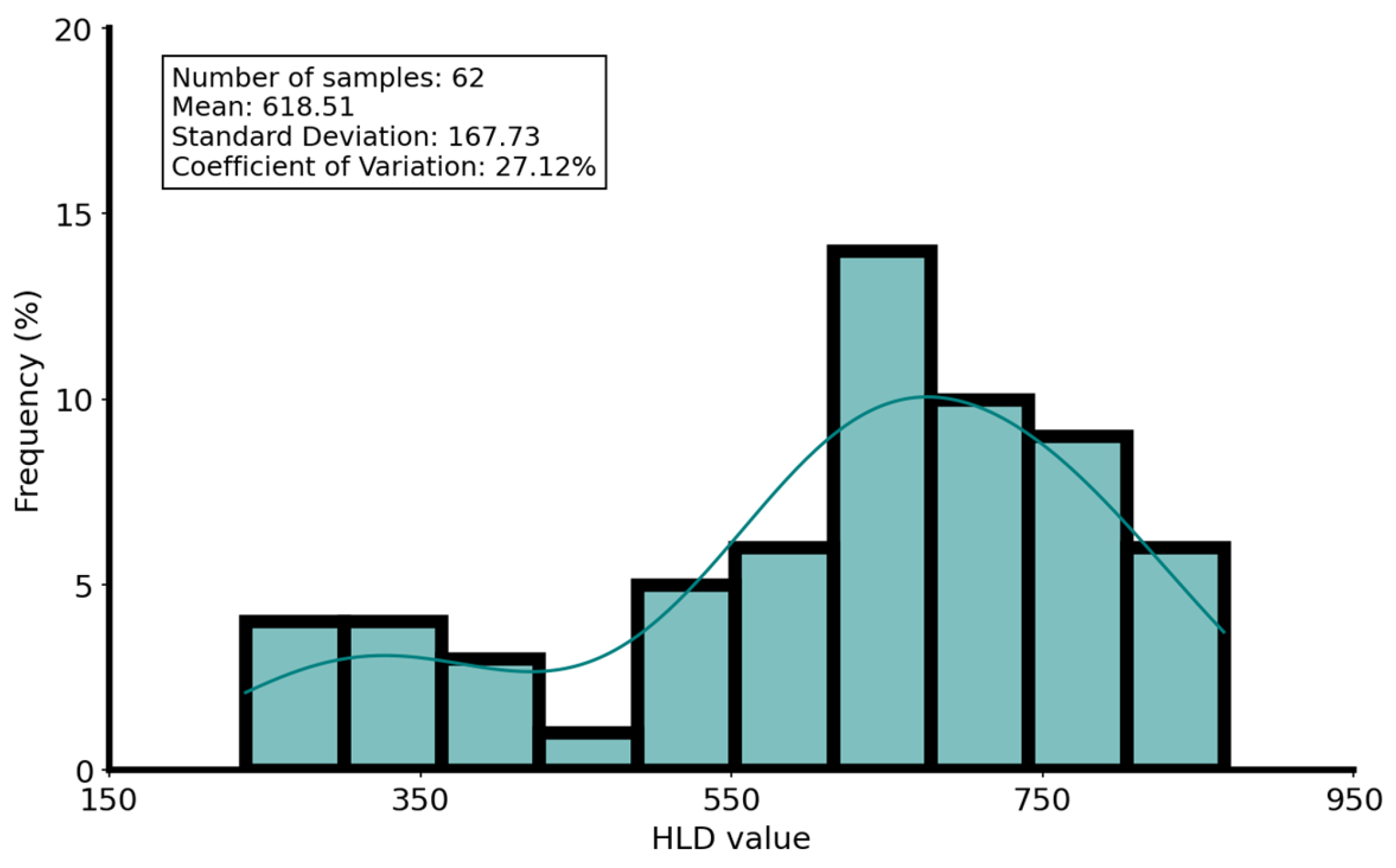
where $N$ denotes the number of required LRH tests to lead the representative mean HLD value, $p$ expresses the precision index as a function of error level, $t_{\beta }$ represents the confidence coefficient obtained for the student $t$ distribution, and ${cv}_{ob}$ is the coefficient of variation for the conducted LRH tests, with an initial value of 5% at the beginning of the test. This study considered a 9.1% error level (representing a precision index of 1.2) and a 95% confidence interval for all rock samples. The LRH measurements were strategically placed to cover the entire rock surface, ensuring no single spot was measured twice and avoiding measurements near the edges. Using a calibration block, the device was calibrated regularly after testing ten consecutive samples or at the beginning of each testing day. The distribution of the measured representative mean HLD values for all 62 rock samples, along with their statistical summary, is provided in Figure 2.

The abrasivity of the rock samples was measured using the CAI test, a destructive testing method. This study used the west version of the CAI device with the styluses having a Hardness of 54 (Rockwell C Scale). The styluses are sharpened carefully after each use. Following the International Society of Rock Mechanics (ISRM) [41], the freshly broken surface for rock samples from the Point Load index test was used for the CAI test. In the case of competent rocks, the samples were cut using a saw-cut machine, and CAI tests were performed on saw-cut surfaces. To account for the smoothness of the saw-cut surfaces, a correction factor of 1.14, as recommended by ISRM, was applied. For each rock sample, the mean CAI value was determined by making seven 10-mm scratches in two perpendicular directions at a constant speed of 1 mm/s. Care was taken to place and lift the Cerchar stylus (Wille Geotechnik, Gottingen, Germany) on and off the rock surface without imposing a dynamic load or causing unwanted wear. At the end of the test, the average CAI value was calculated according to Equation (2):

$$\mathrm{C}\mathrm{A}\mathrm{I}=10\times {\sum }_{i=1}^7{d}_i$$

(2)

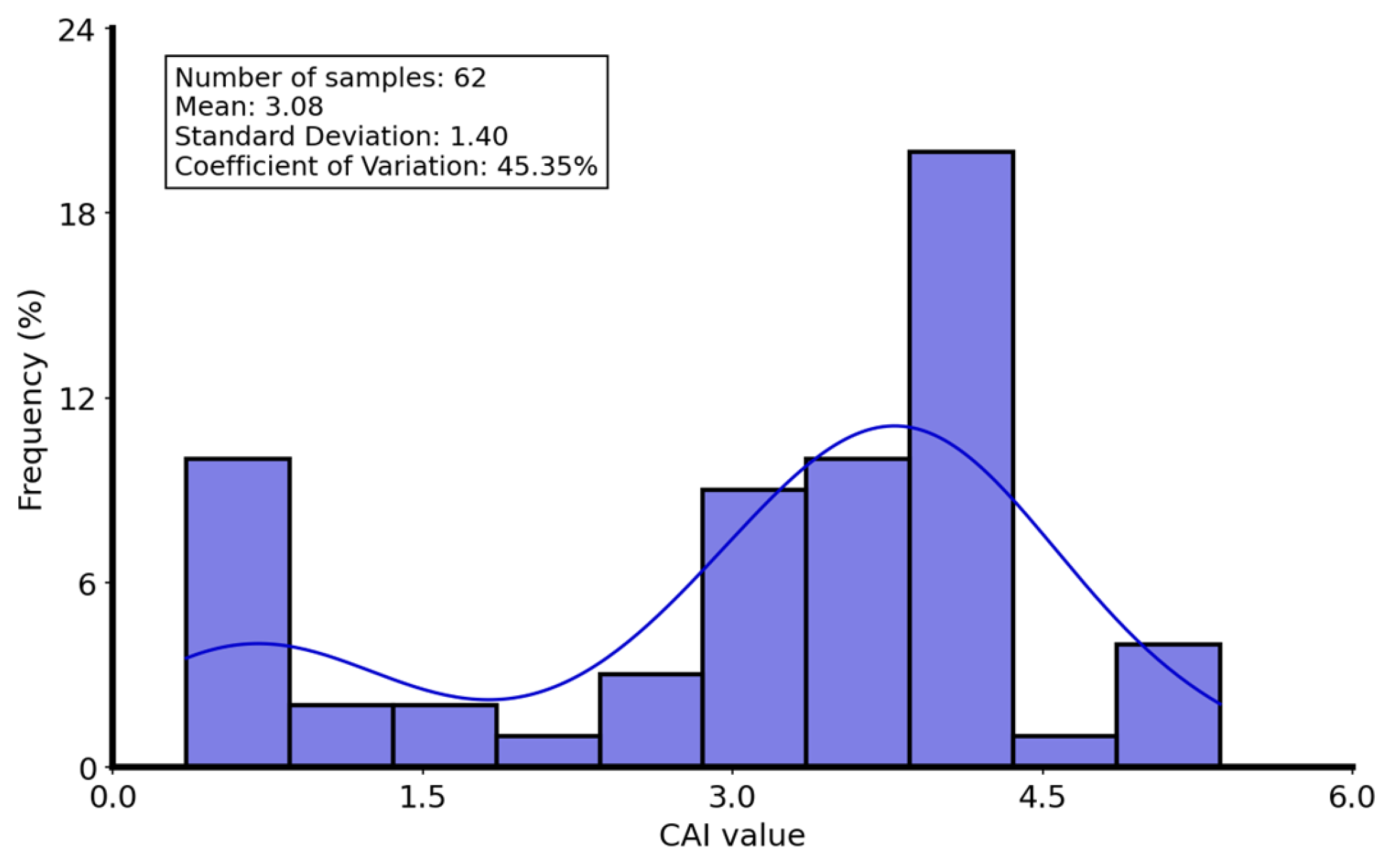
where $d_i$ indicates the average of measured flatness on the stylus tip surface in two perpendicular profiles with an accuracy of 0.01 mm. The optical measurements were performed using a high-resolution calibrated camera mounted on a binocular microscope (Figure 1d). Figure 3 illustrates the distribution and statistical summary of the measured mean CAI values of the collected rocks.

The last stage is performing the BWI test, which is considered expensive, time-consuming (e.g., sample preparation and measurements), and demanding, and which requires a larger volume of samples. The BWI test is the industry-standard method for assessing ore grindability in tumbling ball mills. This locked-cycle laboratory test measures the ball mill grinding energy for a specified ore throughput in kWh/t. The BWI reflects the ore’s resistance to grinding breakage through impact, abrasion, and attrition. The tests were performed using a standard Bond ball mill and following established test procedures (Figure 1e). Individual rock samples were crushed to minus 3.36 mm, 100% particle size passing 6 mesh.

Afterward, since the BWI test requires a minimum volume of feed, the crushed rock samples were mixed based on the gold grade, abrasivity, and the label given by the geologist on the mine site, each weighing at least 7 kg. In total, 10 ore groups were prepared for the BWI test.

Table 2. The characteristics of the rock samples used for Ore 7.

Sample	Rock Type	Weight (g)	Grade (ppm)	HLD	CAI	Work Index (kWh/t)
GS1-24	Sedimentary	1500	2.02	818.25	4.28	18.0
GS1-09	Sedimentary	1500	1.56	577.00	4.29
GS1-21	Sedimentary	1750	0.21	719.06	4.29
GS1-49	Sedimentary	1200	2.69	846.38	4.31
GS1-11	Sedimentary	750	0.60	630.19	4.33
GS2-05	Sedimentary	1200	0.00	747.10	4.01

shows the characteristics of rock samples forming Ore 7 as an example of the mixing strategy. The test was performed to a target grind size of minus 250 µm, 100% product size passing 60 mesh. The BWI tests were conducted at SGS Mineral Services Facilities in Lakefield, Canada.

Table 3. The results of the Bond Work Index test.

Ore Group	Weight (g)	Mesh of Grind	F80 (µm)	P80 (µm)	Gram per Revolution	Work Index (kWh/t)
Ore 1	7200	60	2570	173	1.27	20.1
Ore 2	7150	60	2524	175	1.26	20.5
Ore 3	7050	60	2521	177	1.33	19.7
Ore 4	7050	60	2542	206	1.25	23.1
Ore 5	6900	60	2537	182	1.43	18.9
Ore 6	7400	60	2608	201	1.24	22.7
Ore 7	7900	60	2554	179	1.5	18
Ore 8	7800	60	2551	182	1.56	17.6
Ore 9	8850	60	2432	180	3.19	9.8
Ore 10	7400	60	2389	169	2.3	12.3

presents the results of the BWI for all ten BWI tests given.

2.2. Preprocessing

2.2.1. Geochemical Data

This section details the required preprocessing steps to obtain the reliable features of the pXRF and HSI data. As previously mentioned, the pXRF device can measure the surface concentration of several geochemical elements in each reading. For each rock sample, five pXRF readings were taken and averaged to measure the mean surface concentration of the geochemical elements. A two-step quality control procedure was applied to all pXRF-derived elements. First, the lower detection limit (LDL) was calculated, and the percentage of non-detects was assessed. The LDL is defined as the minimum concentration that the pXRF can reliably detect [57,58]. Second, instrument precision was evaluated using the relative standard deviation (RSD) from replicate measurements on a certified reference material. The eighteenth replicate readings of SRM 2711a were employed to assess the precision and bias of the geochemical elements. The percent difference between the mean concentration of the readings of SRM 2711a and the best values reported by the CRM certificate was used to check the bias of the device. Elements were retained only if (i) more than 50% of their values were above the LDL (indicating adequate detectability) and (ii) their RSD was below 20% (indicating high precision). This filtering ensured that only geochemically meaningful and analytically reliable elements were carried forward [14]. Out of the 40 elements measured by the pXRF, only 15 satisfied both criteria: Al, Ca, Fe, Mg, Si, Ti, Cr, Mn, Ni, Rb, Sr, Zn, Sn, Y, and Zr (

Table 4. The statistical summary of the preprocessing process for pXRF data. LDL: lower detection limit; RSD: relative standard deviation; CV: coefficient of variation.

Geochemical		Lower Detection Limit		SRM 2711a		Readings of Rock Samples
Feature	Unit	Value	<LDL (%)	RSD (%)	Bias (%)	Min	Mean	Max	CV (%)
Al	%	<0.01	0	1.27	18.9	1.14	5.9	11.96	39
Ca	%	<0.01	0	0.54	0.11	0.9	4.9	13.2	55
Cr	ppm	12.84	0.63	11.7	−32.8	66.4	793.1	2682	104
Fe	%	<0.01	0	0.27	1.21	1.02	5.1	11.54	40
Mg	%	0.01	0.78	18.25	16.7	0.68	7.1	18.95	77
Mn	ppm	11.36	0	3.17	9.18	116.2	837.3	1947	48
Ni	ppm	3.08	0.78	9.92	−37.2	7.27	519.3	1987.6	124
Rb	ppm	0.67	6.55	1.04	1.48	1.28	69.6	192.9	73
Si	%	<0.01	0	5.22	4.87	7.04	19.9	29.81	24
Sn	ppm	4.59	5.51	13.54	n/a	20.64	29.3	43.8	16
Sr	ppm	0.37	0	0.65	6.86	15.2	332.5	894.75	61
Ti	%	<0.01	2.36	3	3.17	748.2	3352.5	7632	44
Y	ppm	0.98	5.73	5.03	n/a	1.96	13.24	32	49
Zn	ppm	2.33	0.15	1.03	−11.9	31.6	100.9	188.5	32
Zr	ppm	0.91	0.79	0.61	n/a	7.13	93.5	216	65

).

Although some retained elements (e.g., Cr, Mn, Ni, Rb) occur at trace levels, they were included because they satisfied the detectability and precision criteria and can still provide useful secondary geochemical information. All pXRF measurements were collected from rock surfaces, with five readings per sample, each covering the area of the pXRF device window (≈2 cm²). As a result, the data represent surface geochemistry rather than full bulk composition. Because the goal of the study was to evaluate whether rapid, preparation-free pXRF measurements under real mining conditions can provide meaningful relationships with rock properties, surface measurements on unprepared samples were used.

2.2.2. Hyperspectral Data

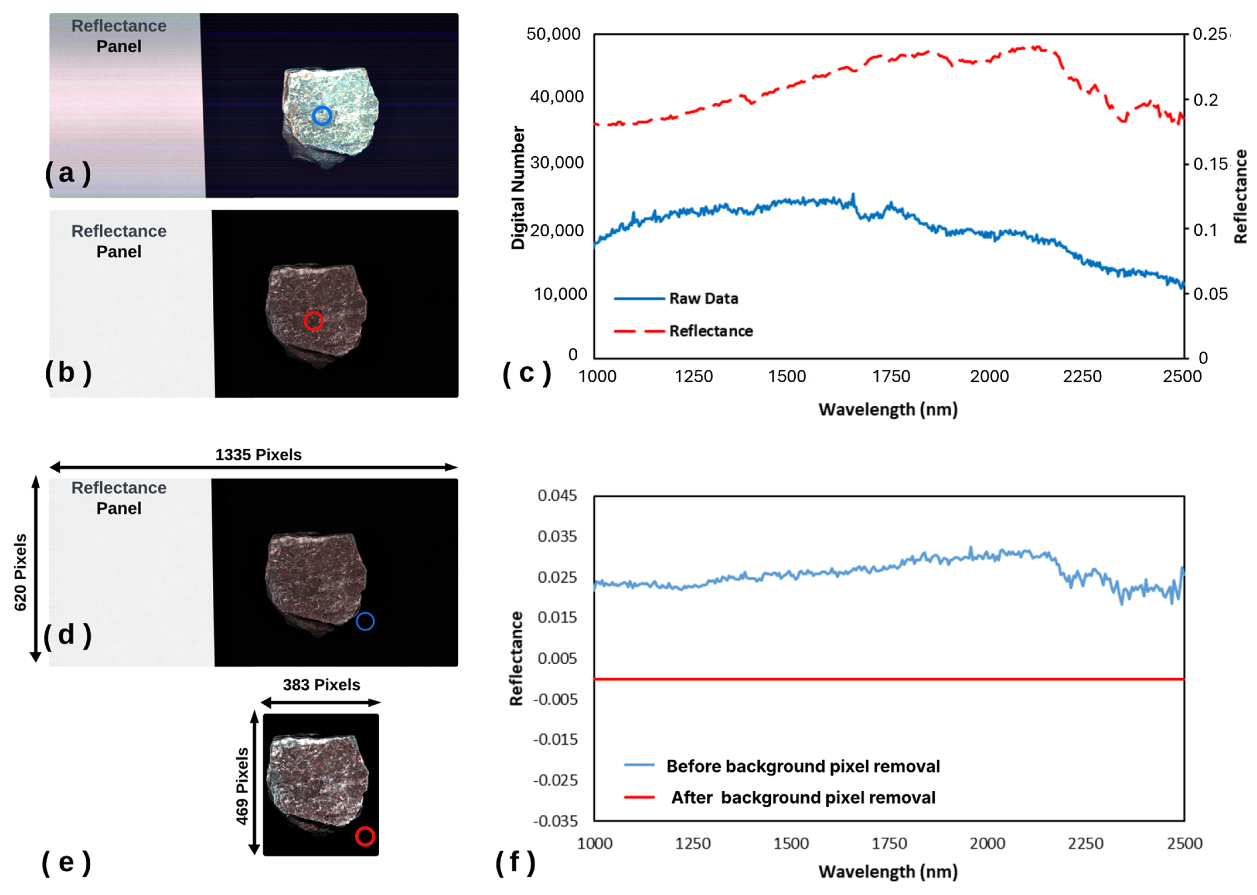
The preprocessing of raw SWIR hyperspectral data involved three main steps. First, radiometric correction was applied to convert raw digital numbers (DN) into radiance using camera-specific radiometric calibration based on the camera manufacturer’s calibration, and then it was converted to reflectance using the spectral reference target. Second, that integration time and scanning speed were adjusted to match the sample albedo and illumination intensity in order to minimize the oversaturation in scenes. The occurrence of oversaturated pixels, often caused by high albedo contrasts within samples, was identified, masked, and removed. Finally, background spectra were eliminated by cropping each image to include only the rock sample, thereby minimizing file size. For more detailed information regarding scanning conditions and preprocessing procedures, see [50]. Figure 4 demonstrates the preprocessing steps applied to one of the samples.

2.3. Feature Engineering

The preprocessed SWIR images contain a large number of pixels, depending on the size of the rock samples and scanning distance, each representing the spectral curve at a specific location on the scanned rock sample. One of the biggest challenges in working with this data type is extracting the most essential and reliable features. This study employs the two feature extraction approaches proposed by Ghadernejad and Esmaeili [50] and Ghadernejad et al. [52] to extract the spectral features.

2.3.1. Band Ratio

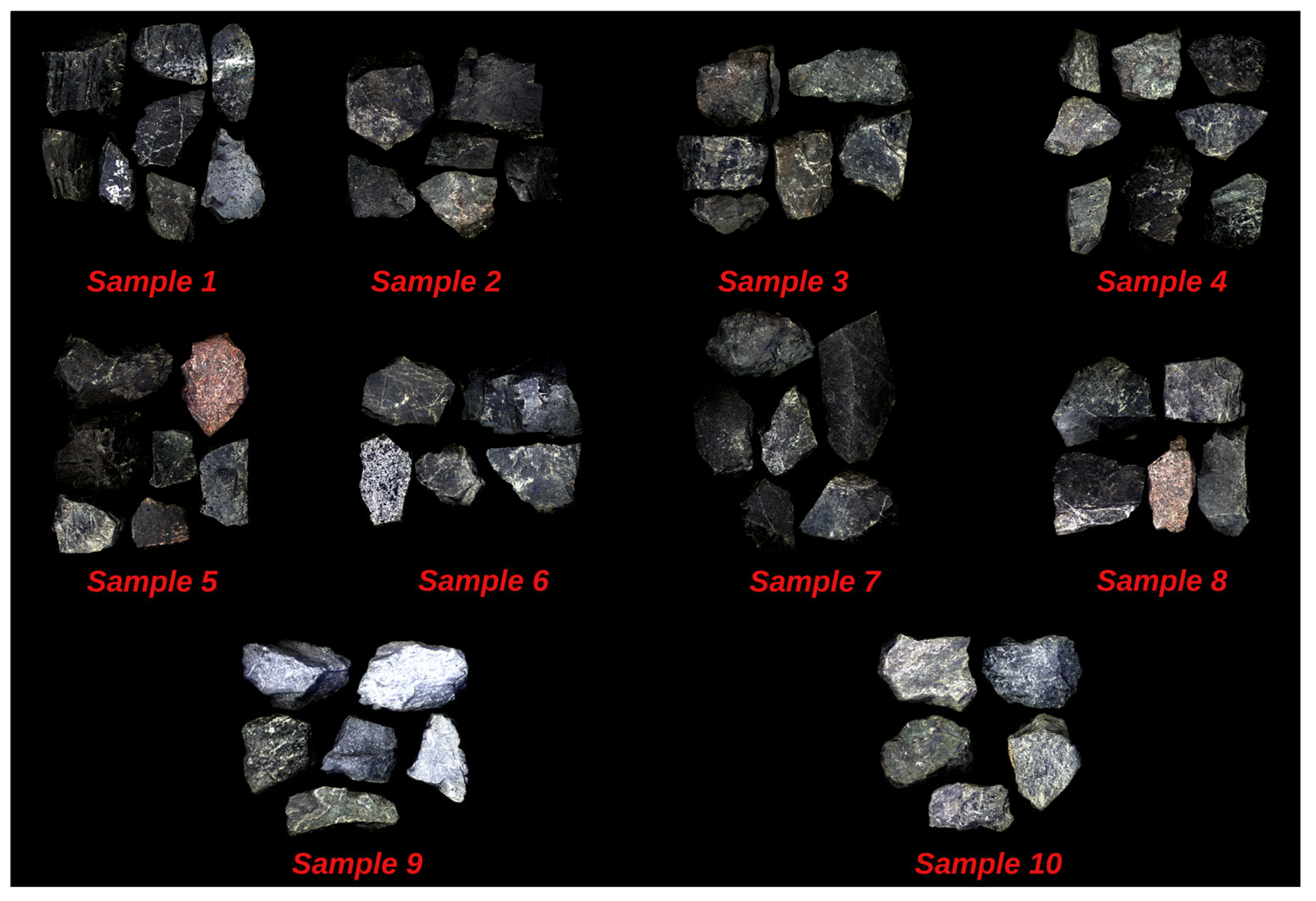
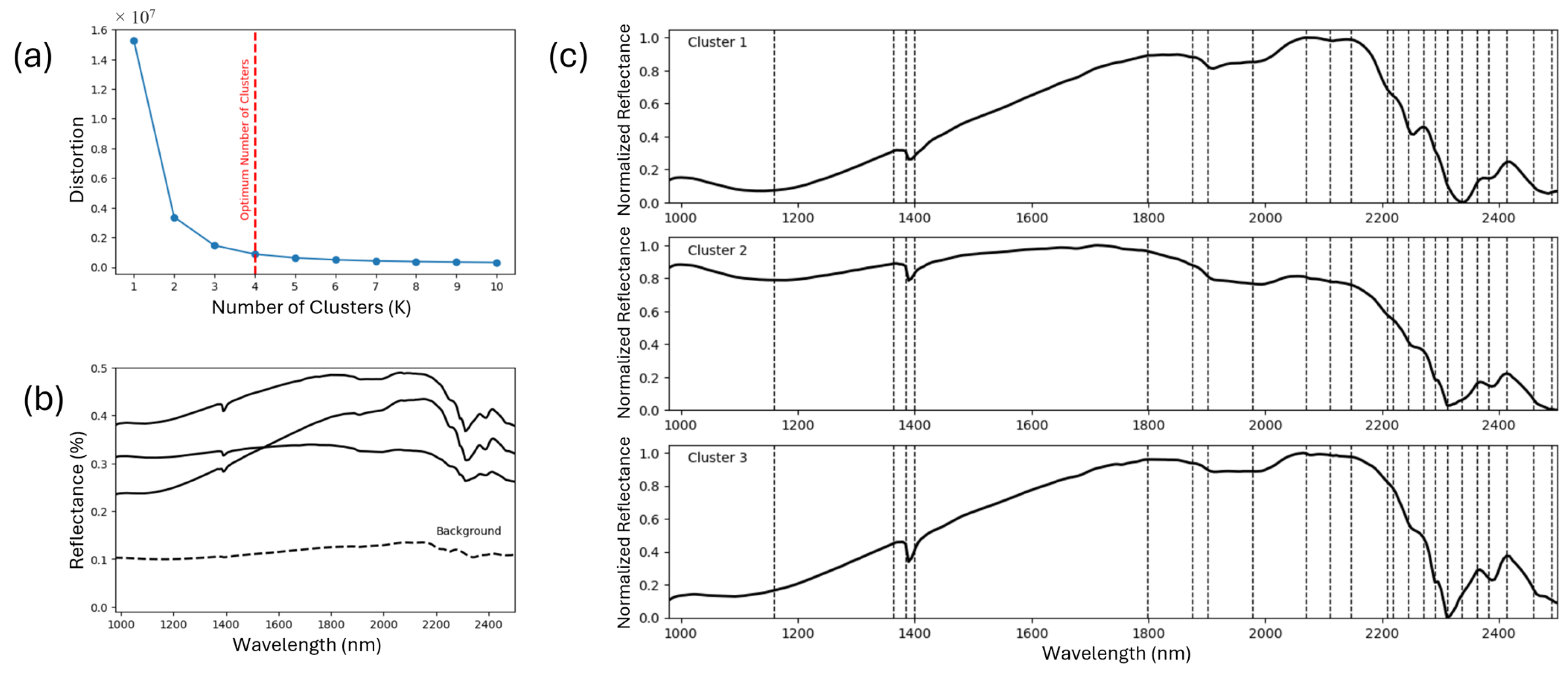
Ghadernejad and Esmaeili [50] proposed a spectral feature extraction approach that applies the band-ratio concept to the mean spectra obtained from K-means analysis. The first step in this feature extraction approach is to mosaic all SWIR images together, ensuring that the spectral curves of all SWIR images are compared (Figure 5). It must be noted that the rock samples in each ore group are placed close to each other in the final mosaic image. This primarily aids in visualization and does not impact the final results, as each spectrum in the mosaic image is analyzed individually. Before conducting the K-means clustering analysis, an attempt was made to normalize all spectral curves, which is of great importance since the K-means algorithm clusters spectral curves based on shape and intensity. In such a case, the clustering will only be based on the difference in the shape of the spectral curves. The clustering analysis starts with determining the optimal number of clusters using the elbow method.

Consequently, multiple K-means analyses were conducted with cluster numbers varying from 2 to 10. Figure 6a shows that the K-means clustering with 4 clusters most effectively captures the dominant spectral curves. The mean spectral curves obtained from the K-means clustering with 4 clusters are depicted in Figure 6b. It is important to note that one of these spectral curves corresponds to the image background and was excluded from the analysis.

After obtaining the dominant spectral curves from the K-means analysis, all three spectral curves were thoroughly examined for the spectral features. A spectral feature was defined as a band ratio, reflectance at band i divided by reflectance at band j, whenever a change was detected in the curves. Figure 6c illustrates the feature extraction process.

Table 5. The obtained band ratios from the feature extraction approach. The numbers represent wavelength in nm.

Features	Band1	Band2	Features	Band1	Band2
Band Ratio 1	1159	1364	Band Ratio 9	2336	2310
Band Ratio 2	1394	1798	Band Ratio 10	2361	2336
Band Ratio 3	1978	2070	Band Ratio 11	2413	2382
Band Ratio 4	2208	2147	Band Ratio 12	2361	2382
Band Ratio 5	2244	2208	Band Ratio 13	2461	2413
Band Ratio 6	2244	2269	Band Ratio 14	2413	2459
Band Ratio 7	2208	2269	Band Ratio 15	2489	2459
Band Ratio 8	2269	2310

provides details on the obtained band ratios for further analysis. Subsequently, this approach was applied to all rock samples, reducing the spectral dimensionality from 298 to 15. For each sample, the primary representative feature values were calculated as the mean of the features across all pixels.

2.3.2. Absorption Peak

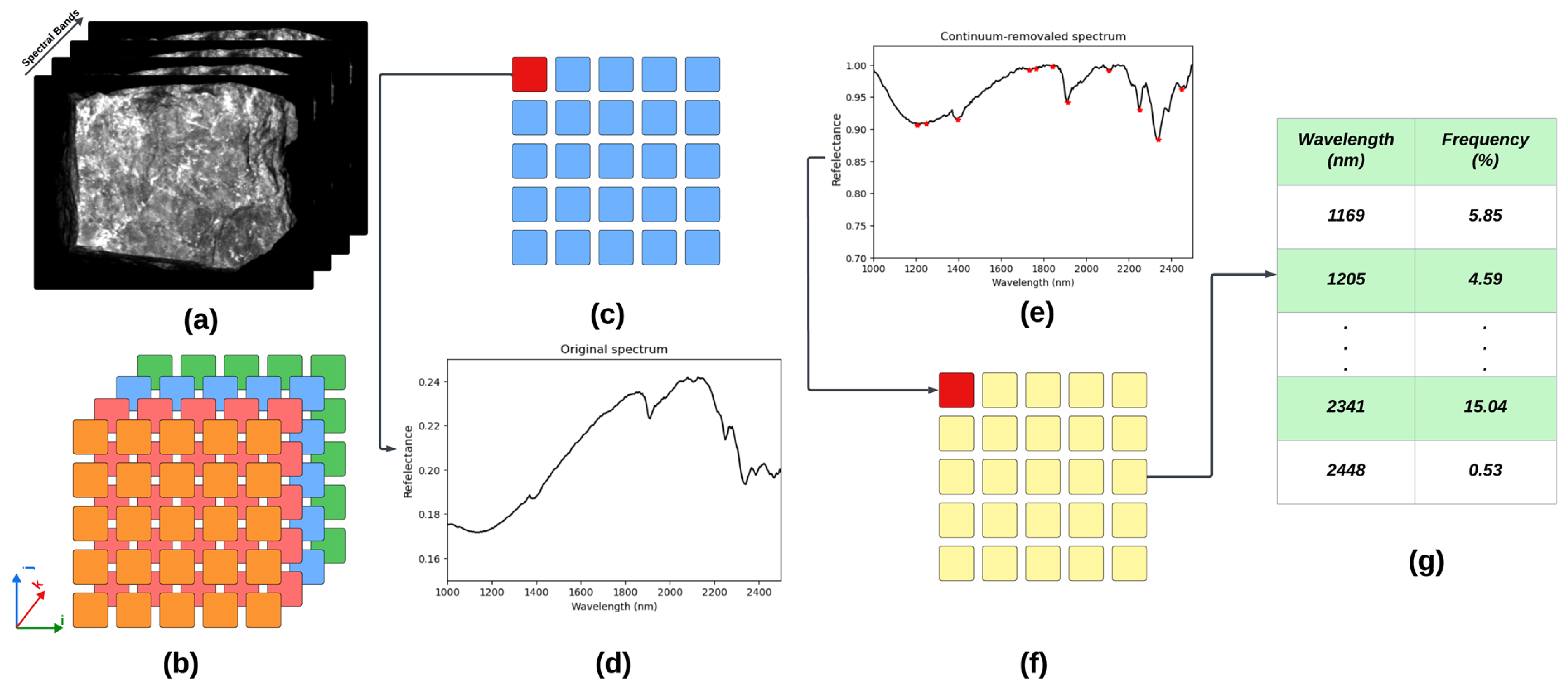
In another study, Ghadernejad et al. [52] proposed an automated feature extraction based on the absorption peak concept. An absorption peak is a distinct feature on the spectral curve where there is a notable decrease in reflected electromagnetic radiation at a certain wavelength. The suggested method calculates how frequently the absorption peak occurs for a specific wavelength across all pixels in a rock sample. It assesses the percentage, ranging from 0 to 100, of occurrences of an absorption peak at that specific wavelength for the rock sample.

Figure 7 outlines the step-by-step method for extracting absorption peaks. Initially, a continuum removal function is applied to each pixel by fitting a convex hull over the spectrum, using straight-line segments to connect local spectral maxima. Following this, the method examines the spectrum for absorption peaks by detecting changes in the sign of the derivative at each wavelength. An absorption peak is identified when the spectral slope transitions from negative to positive. This procedure is executed for all pixels, with the results saved as tabular data that is suitable for developing machine learning predictive models.

2.4. Statistical Analysis

In this study, two nonparametric statistical methods were used to assess the ability of the testing methods to characterize grindability behavior: the Mann–Whitney U test for differences in central tendency between independent samples and the Kolmogorov–Smirnov (KS) test for distribution discrepancies. They were selected due to their ability to work with non-normal distributions and handle unequal sample sizes in datasets.

The Mann–Whitney U test is a non-parametric statistical method used to compare two independent samples that may not follow a normal distribution. Also known as the Wilcoxon rank-sum test, it is a nonparametric alternative to the independent samples t-test used when data do not meet the normality assumptions required for a t-test. Instead of directly comparing means, the test evaluates differences in the central tendency by ranking all observations across both groups and then comparing the distributions of these ranks. This makes the Mann–Whitney U test particularly suitable for datasets that are skewed, contain outliers, or have unequal sample sizes, where traditional parametric tests such as Student’s t-test may not be appropriate. The test assumes that observations are independent and that the dependent variable is at least ordinal in scale [59,60,61]. In practical applications, the null hypothesis states that the two groups are drawn from identical populations, implying no systematic difference in their medians. A statistically significant result indicates that one group tends to have systematically larger or smaller values than the other [62].

KS test is a non-parametric procedure used to determine whether two samples originate from the same underlying distribution. Unlike the Mann–Whitney U test, which focuses primarily on median differences, the KS test compares the entire cumulative distribution functions (CDF) of the two samples. The test statistic is defined as the maximum absolute difference between the two empirical CDFs. This feature makes the KS test sensitive not only to shifts in location (central tendency), but also to differences in spread, skewness, and overall distributional shape [63]. Under the null hypothesis, the two samples are assumed to follow the same probability distribution. Rejection of the null indicates that at least one aspect of the distribution—such as dispersion, skewness, or tails—differs significantly between groups. This test has been widely adopted in fields such as environmental sciences, mining, and remote sensing to compare geochemical or geophysical measurements across different sampling domains. Its non-parametric nature makes it robust for exploratory data analysis where distributional assumptions are uncertain or violated [64,65].

3. Results

This section evaluates the potential applications of the mentioned testing methods in characterizing the ore grindability. Rather than utilizing the obtained data to establish linear and non-linear relationships to estimate the BWI value, the measured data were used to distinguish different ore grindability behaviors. We selected a classification-based approach because the distinct grindability behaviors, when combined with ore grade and size distribution data, will inform downstream process planning and optimize comminution strategies.

The threshold selected for distinguishing different grindability behaviors in this study aligns with the existing grindability observed in mines under investigation, as discussed below. The preliminary grindability study conducted for pit 1 in 2008 included 14 BWI tests and showed that the rock displays moderate to relatively hard characteristics, with grindability values ranging from 14.6 kWh/t to 18 kWh/t, averaging 16 kWh/t. Recognizing the need to extend the comminution circuit design, another BWI testing program was implemented in 2011, consisting of 59 samples collected from both pits. The results revealed a decrease in the average BWI to 15 kWh/t, along with a drop in the minimum BWI from 14.6 kWh/t to 11.1 kWh/t. Based on this dataset and the mine’s operational practices, ore material is classified into two classes: BWI < 15 kWh/t as moderate, and BWI > 15 kWh/t as hard. This site-specific threshold was therefore adopted to ensure consistency with established operational definitions and comminution design criteria.

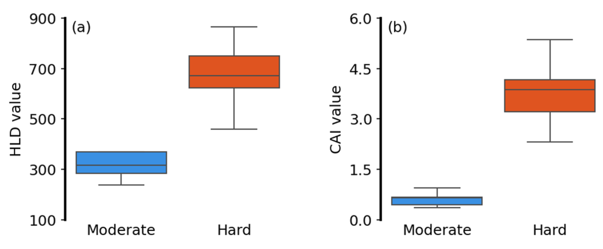
Figure 8 illustrates how the two mentioned grindability behaviors, moderate and hard, can be distinguished using the mean HLD and CAI values using box plot visualization. The horizontal axis indicates the observed grindability behaviors within the tested ore groups, while the vertical axes show the mean HLD and CAI values measured for the tested ore groups. It should be noted that the HLD and CAI values of all rocks within each ore group were used to generate the boxplots. The corresponding graph to the HLD (Figure 8a) demonstrates a clear trend: the moderate class exhibits a low mean HLD value of approximately 300, whereas hard ores show significantly higher mean HLD values, ranging from 500 to 880, with an average of around 650. The obtained result suggests that the mean HLD value effectively distinguishes the moderate class from the hard class.

The result for the mean CAI values reveals that the ore groups with moderate grindability have the lowest mean CAI value at around 0.7, with a maximum of 1. On the other hand, the hard materials show higher abrasivity values, ranging from 2.8 to 5.2. The performance of the mean CAI value in characterizing the grinding behaviors mirrors the trends observed with the mean HLD value. These findings imply that the CAI data can be used to differentiate the ore material, which shows different grindability behaviors. No overlap was observed between the range of HLD and CAI values measured for ore groups with different grindability behaviors, suggesting a strong discrimination potential of these testing methods, at least in the case of this study.

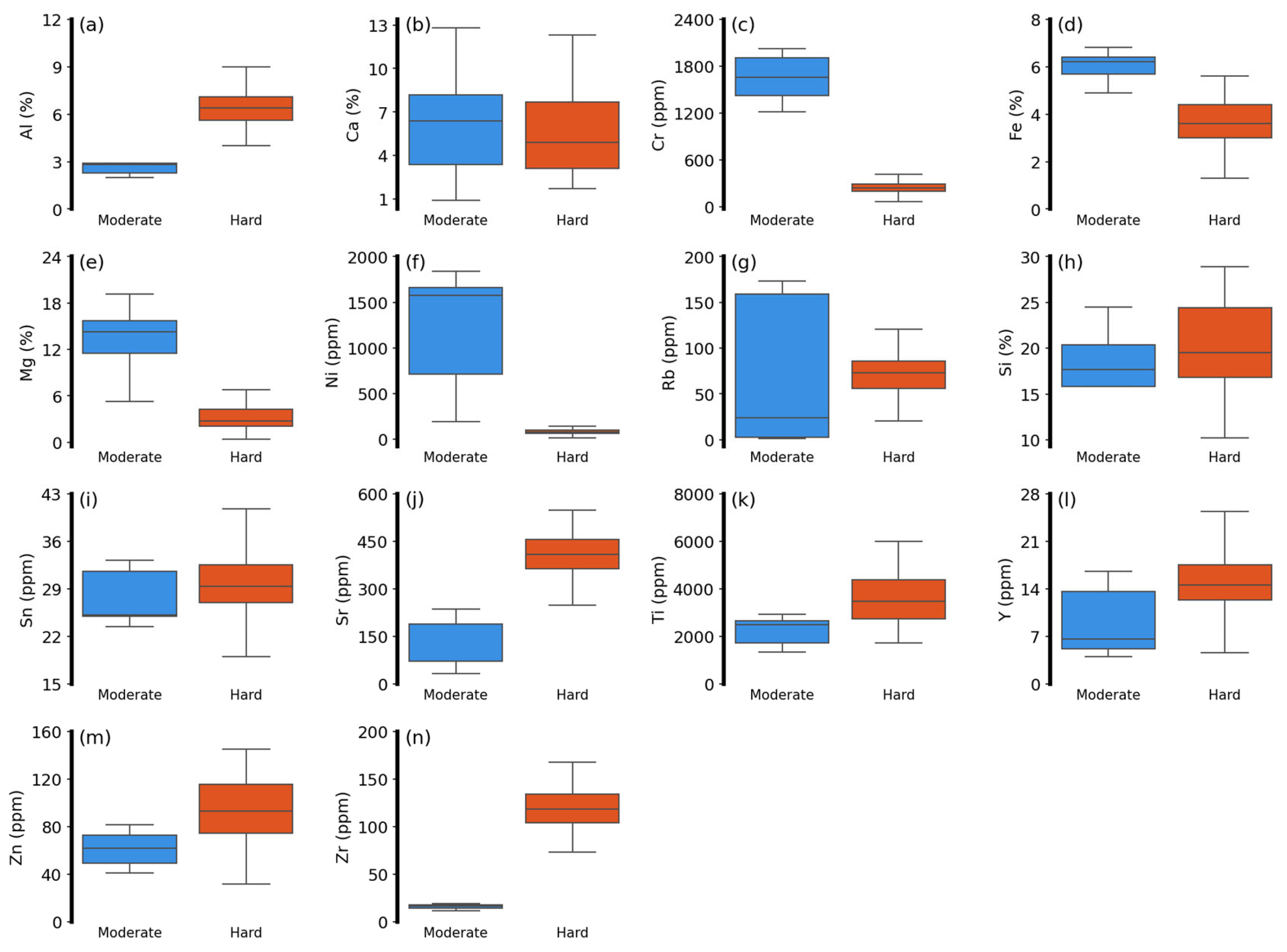
While HLD and CAI directly measure mechanical properties, the geochemical and SWIR datasets provide indirect proxies linked to mineralogy, which also influences grindability behavior. The same procedure was applied to the geochemical data. Figure 9 examines the extent to which geochemical features can differentiate the grindability behaviors of the ore groups. The analysis reveals that Al, Cr, Mg, Ni, and Zr can effectively separate the moderate BWI class from the hard BWI material. This finding aligns with the trends observed in the mean HLD and CAI values. Furthermore, other geochemical features such as Fe, Sr, and Y exhibit weaker potential for discriminating ore grindability behaviors than the previously mentioned features. Unlike the HLD and CAI, the geochemical features can also be used to link the material hardness to the rock types, which will be discussed later.

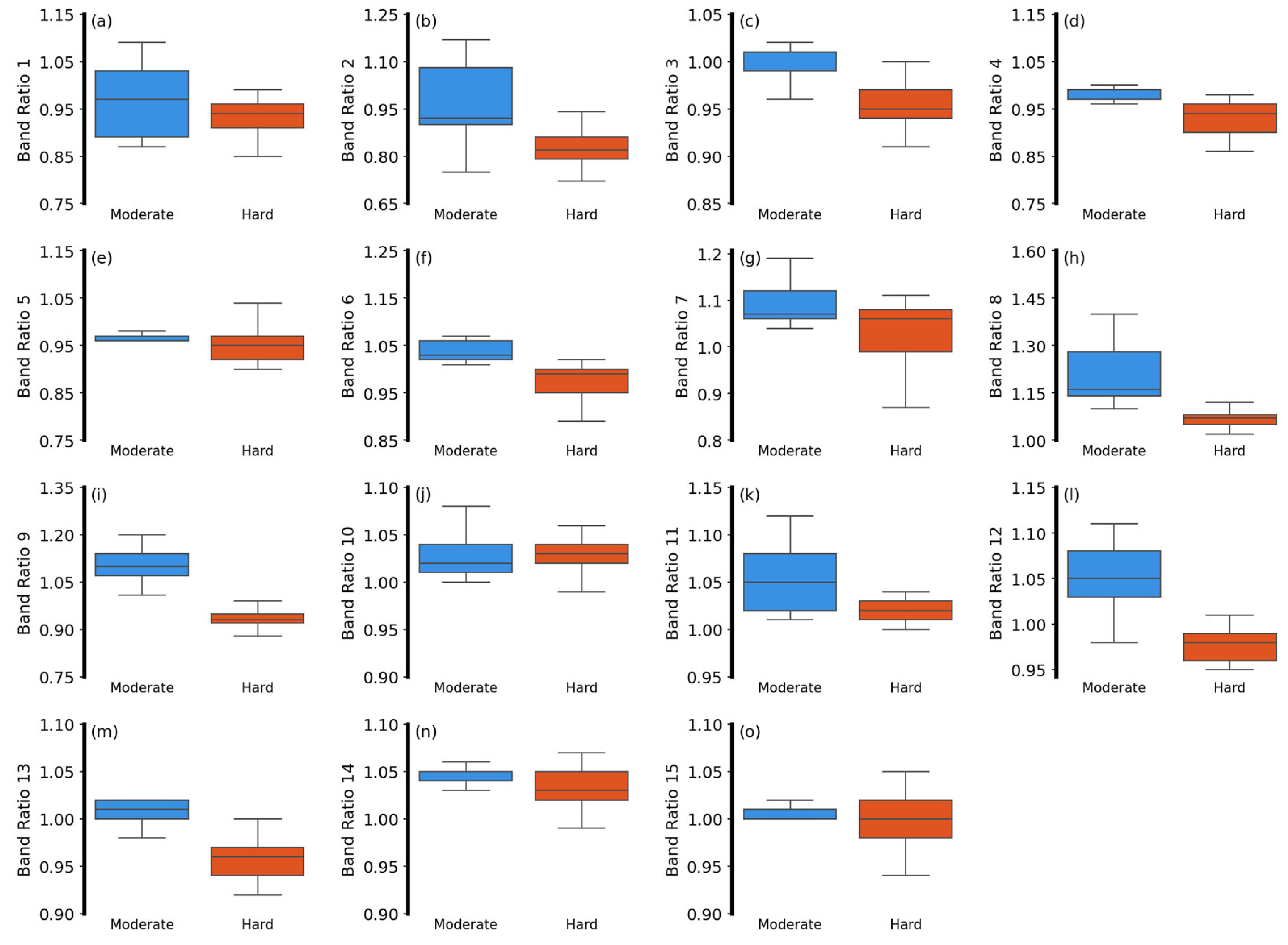
The final step of analysis is dedicated to investigating the use of SWIR data to discriminate between different grinding behaviors of the tested ore groups. As was mentioned, this study employs two different spectral feature extractions. Figure 10 illustrates the relationship between different band ratios and grindability behaviors of the ore groups. It is important to note that, due to the band ratio concept used to define these spectral features, spectral feature values typically range from 0.8 to 1.2. Like the geochemical data, certain spectral features, including band ratios of 4, 6, 8, 9, and 13, demonstrate the potential application in differentiating between grindability behaviors, with the strongest discriminative potential observed for band ratio 9, clearly distinguishing between different grindability behaviors.

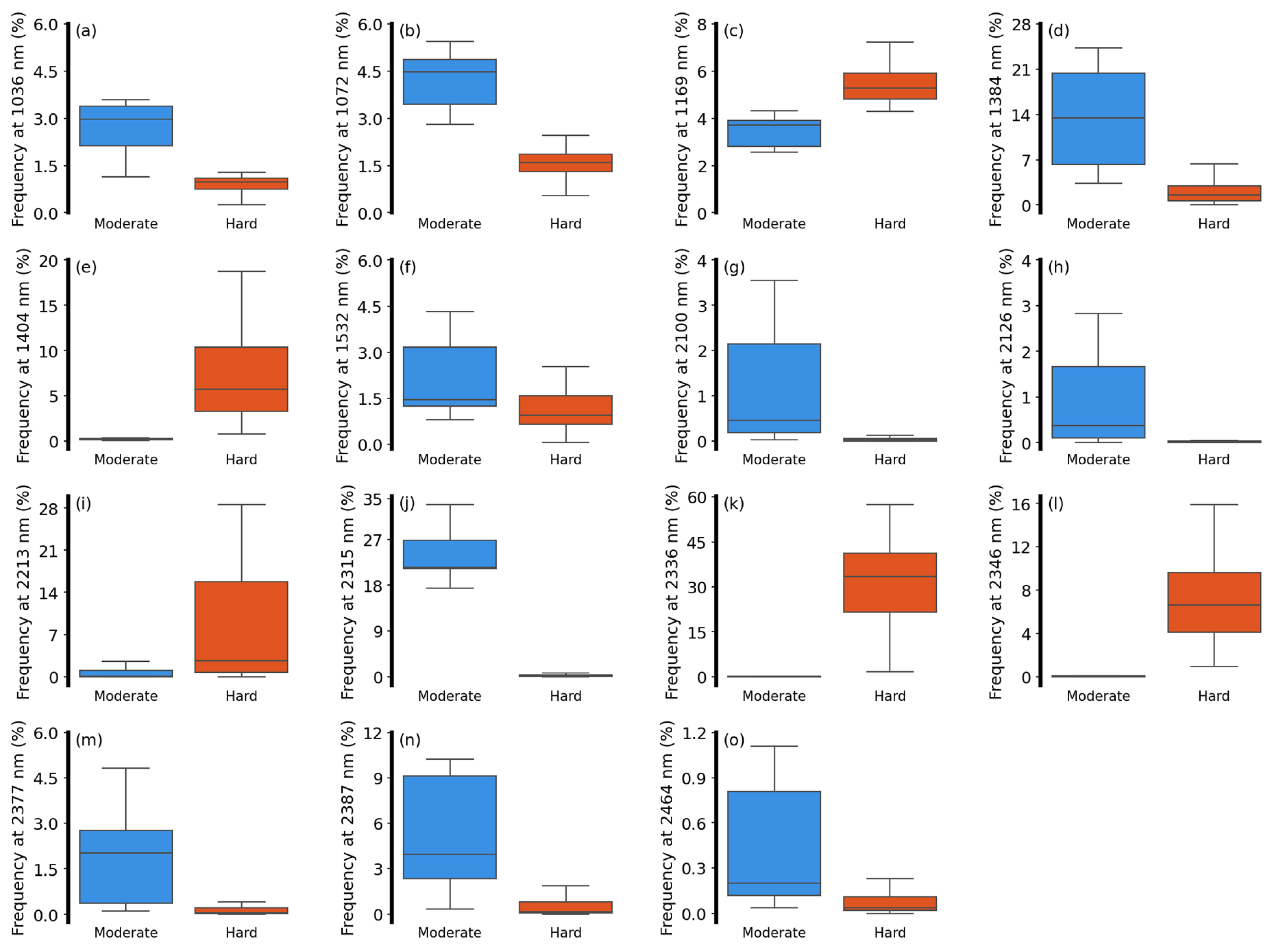
On the other hand, the spectral features resulting from the absorption peak concept were also applied to each rock sample within the ore group and used to investigate the grindability behaviors of the studied ore samples (Figure 11). The results showed that some of the absorption-based spectral features, such as the frequency of absorption peaks at 1072, 1169, 1404, 2315, and 2346, can effectively separate the moderate class from the hard material. Unlike the band-ratio approach, the spectral feature obtained from the absorption peak approach could be related to certain geochemical compositions. For example, a strong absorption peak around 2200 nm could be associated with Al-OH in the rock [66]. Ultimately, this aims to gain a better understanding of the characteristics of the ore groups being tested.

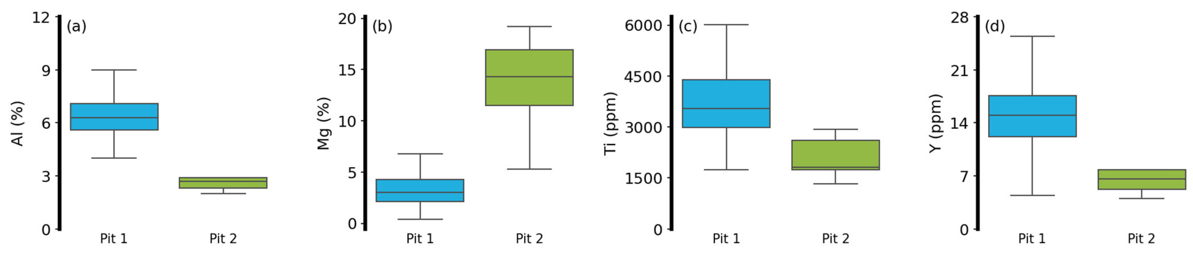
As previously mentioned, given the significant potential of geochemical features in characterizing the grindability behaviors of ore groups, investigating the links between rock types and their grindability could enhance decision-making related to optimizing the comminution process. These geochemical distinctions are closely tied to the predominant rock types within the studied open pits. Figure 12 demonstrates the distribution of some of the geochemical features that show a strong potential in discriminating grindability behaviors for the two studied pits. For example, Al concentrations in the rock samples collected from Pit 1, mostly including greywackes, are generally higher than those collected from Pit 2, which mainly include ultramafic rock. This elevated Al content correlates with harder grindability behavior.

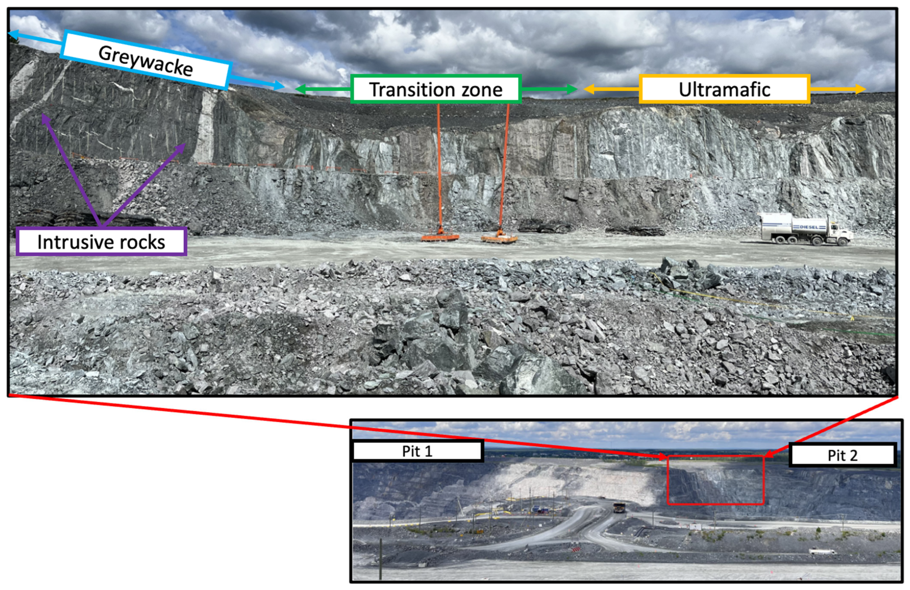
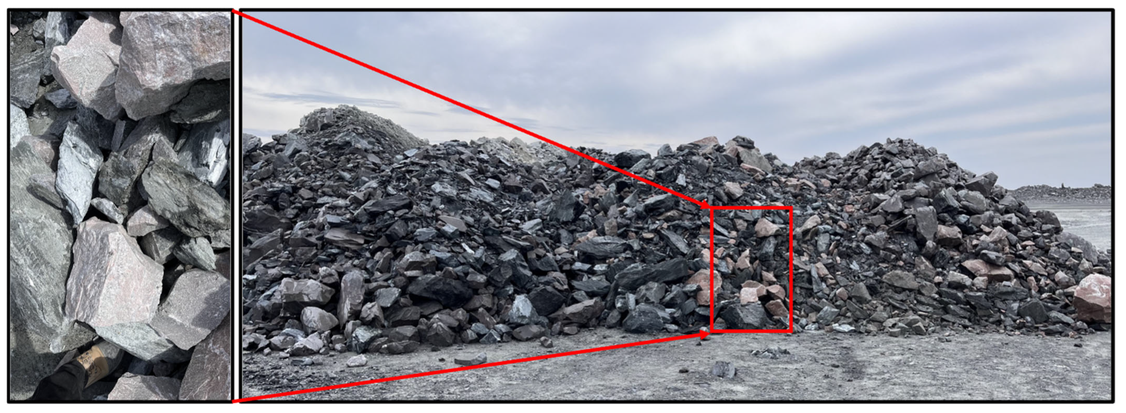
In relatively straightforward geological settings, a geologist could leverage lithological cues, such as recognizing greywacke versus ultramafic units, to infer differences in grinding behavior. However, relying solely on traditional field-based methods becomes challenging in more geologically complex scenarios, such as contact zones where lithological boundaries are less distinct. Figure 13 depicts a contact zone observed in Pit 2, which includes greywackes, intrusive rocks, and altered ultramafic rocks. In such a case, different rock types will be mixed after the blasting, which makes it challenging to determine the ore behaviors in the comminution process. Figure 14 shows the distribution of rocks sourced from such a complex zone after blasting at the stockpile.

Table 6. Description and average occurrence of the observed ore types in the two studied pits, provided by the mine.

Ore Type	Average Occurrence
	Pit 1	Pit 2
Carbonatized porphyry	14%	16%
Silicified and potassicly altered porphyry	9%	5%
Slightly altered greywacke	12%	25%
Carbonatized greywacke	52%	29%
Silicified and potassicly altered greywacke	13%	2%
Carbonatized ultramafic	N/A	4%
Talc-chlorite schist	N/A	21%

provides the average occurrence of different ore types within the studied pits. As shown in Table 6, most of the ore types can be found in both pits. Combining the ore type distributions with the complexity of the geological setting further underscores the challenges of relying solely on traditional field-based methods to characterize ore variability within the mine.

To complement the graphical comparisons, we applied statistical tests to verify whether the observed differences were significant. While visual inspection of boxplots provides an intuitive understanding of potential disparities, statistical tests are necessary to objectively confirm these differences. In this study, the Mann–Whitney U test was applied on destructive and non-destructive tests, and results consistently indicated large and statistically significant differences across the investigated parameters (p < 0.001 for all cases). For LRH and CAI, class Hard exhibited substantially higher median values relative to class Moderate, with Cliff’s delta values approaching 1.0, denoting an almost complete separation between the two distributions. The same pattern was observed for Al concentrations from the pXRF data, and for the hyperspectral absorption peak position at 1404 nm, where class Hard values were systematically greater than those of class Moderate. In contrast, the hyperspectral band ratio 9 displayed the opposite trend, with Group Moderate showing markedly higher values (Cliff’s delta = −0.970). These large effect sizes highlight the robustness of the contrasts in central tendency, indicating that the two grindabilities of the ore samples being tested differ in systematic and interpretable ways.

In addition, the KS test confirmed strong distributional differences across all parameters (p < 0.001). The D statistics were uniformly high (>0.90), with CAI and Al concentration yielding a maximum separation (D = 1.000), indicating that the two grindability behaviors of the ore samples being tested are completely distinct in terms of distributional shape. For LRH and absorption peak at 1404 nm, large D values (0.909–0.911) similarly demonstrated pronounced divergence. The band ratio 9 parameter followed the same pattern, with class Moderate exhibiting higher values and a KS statistic of 0.909. Together, these results provide compelling evidence that the selected destructive and non-destructive tests not only distinguish between the two grindability behaviors in terms of central tendency but also differ across the broader characteristics of their distributions, including spread and skewness.

4. Discussion

The results showed that all four geomechanical and geochemical testing methods could be utilized to differentiate the grindability behaviors of the ore groups being studied. This section evaluates the practicality and resolution of the information obtained from each testing method for potential implementation in the mining operation.

LRH is a fast, non-destructive, portable testing method that provides local information about the hardness of rock samples. It can be used to measure the hardness of different parts of a rock pile without the need for sample preparation and preprocessing steps. However, due to the need for direct and constant contact between rocks and the device’s probe, it is impossible to automate the ore hardness measurement and obtain variability. Even so, the measured variability is not spatially quantified; therefore, the rock pile will be treated as a unit. Integrating the obtained grindability variation with other geometallurgical variables, such as the grade and its variation on the rockpile, will be challenging. On the other hand, CAI is a destructive, costly, time-consuming testing method, requiring rigorous sample preparation and testing procedures that provide local information. These conditions, alongside the challenges discussed for LRH tests, make it impossible to automate grindability characterization for the newly blasted rock piles or stockpiles using CAI testing methods.

The pXRF device offers a fast, non-destructive, portable approach for measuring the concentration of several chemical elements, which can be further used for characterizing the grindability behavior of ore groups, as shown in this study. Although the measuring approach requires no sample preparation, the operator must go to the area of interest on the newly blasted rockpile or step on the stockpile, which could pose a safety hazard to the operator and cause an interruption in the mining process. The obtained reading is local; therefore, numerous readings must be done in different parts of the pile to measure the surface concentrations and their variabilities. Recently, efforts have been made to integrate the XRF devices on the shovel’s buckets to provide real-time ore grade control [67] by streamlining the data collection and preprocessing steps. In such contexts, the gradability behavior derived from geochemical data can be effectively integrated with ore grade, thereby providing more comprehensive insights into ore variability. It is noteworthy that, at the time of this study, the application of pXRF technology mounted on the shovel’s bucket for ore grade control is primarily limited to copper. Furthermore, this integration currently lacks several essential geometallurgical variables, such as particle size distribution and mineralogical composition, which can significantly influence comminution and downstream processes.

Lastly, HSI allows for the rapid acquisition of extensive surface data from a safe distance, thereby minimizing the need for direct contact with potentially hazardous environments. Unlike pXRF, which offers local measurements, hyperspectral imaging delivers spatially continuous data, covering large areas with high spectral resolution. However, the complexity of the collected data necessitates the use of advanced preprocessing and analysis techniques to extract the most reliable and robust spectral features. Recent advancements in airborne-, drone-, and ground-based hyperspectral systems have improved data acquisition and processing efficiency, facilitating real-time decision-making in the field. Regarding hyperspectral scanning, rather than extracting or analyzing mineral-specific spectral signatures at the grain scale, the focus was on general trends and dominant features in the average spectra obtained from particle surfaces. While surface roughness and uncontrolled illumination can affect reflectance intensity and the shape of absorption peaks, these effects are likely to influence all particles in a similar way. Similarly, although particle size can cause beam scattering and reduce infrared absorption intensity, the analysis emphasizes relative spectral behavior rather than precise mineral absorption positions. Consequently, the approach remains robust under the natural scattering and diffuse reflection conditions inherent to the experimental setup.

To provide mineralogical context for the observed BWI trends, a limited number of representative samples from ore groups 1–10 were analyzed using X-ray diffraction (XRD). Although the number of XRD analyses is insufficient to establish quantitative, sample-by-sample correlations across all groups, the results provide qualitative validation of the dominant mineralogical components, including Quartz, Biotite, Muscovite, Chlorite, Dolomite, Calcite, Pyrite, Talc, Magnetite, Hornblende, Albite, and Potassium Feldspar. For example, two ultramafic-rich samples from Ore group 9 contained approximately 23% and 36% Talc, and 33% and 29% biotite, respectively. Both are soft, ductile minerals that explain the lowest measured Bond Work Index (9.8 kWh/t) in this group compared with other mixed ore groups. The samples contained only 1% and 4% Quartz. Additionally, XRD analysis of two samples from ore groups 4 (BWI 23.1 kWh/t) and 6 (BWI 22.7 kWh/t) indicates 20% and 19% Quartz, 22% and 38% Albite, and 43% and 12% Potassium Feldspar, respectively. These minerals have higher hardness (6–7 on the Mohs scale), explaining the higher BWI values measured for these ore groups. These observations illustrate that even limited mineralogical information can help interpret spectral features and grindability trends, providing a practical, operationally feasible framework without requiring extensive laboratory analyses for all samples.

Among the employed testing methods, HSI demonstrates significant potential for further implementation in an active mining environment. One critical advantage of HSI lies in its capability to acquire comprehensive mineralogical data from rock surfaces remotely. In contrast to point-based techniques, such as pXRF, HLD, and CAI, it facilitates the mapping of extensive areas with high spatial and spectral resolution. It detects subtle variations in mineral composition without necessitating direct contact with samples. In addition to determining the grindability behavior of the ore, hyperspectral imaging can be used to determine other geometallurgical variables. It can be used to determine the ore grade, which is not limited to a particular commodity [53]. It can also be used either solely or in integration with another imaging technique, such as Lidar, to determine the particle size distribution on the mine site. These capabilities can be particularly valuable in mine-to-mill optimization, given that grindability is influenced by a range of factors—including ore hardness, particle size distribution, mineralogy, and grade—all of which can be potentially inferred from hyperspectral/Lidar measurements.

On the other hand, although methods like MWD primarily capture the hardness dimension and may miss other critical parameters, such as particle size or grade, their results can be integrated with the information obtained from HSI. In this case, mine planners can build a more comprehensive picture of the geometallurgical characteristics of the orebody, leading to more precise comminution strategies and improved performance. Beyond comminution, hyperspectral imaging presents significant potential for optimizing flotation processes, particularly in identifying deleterious minerals such as clays. As demonstrated by Chen and Peng [68], clay minerals, such as kaolinite, smectite, and illite, adversely impact flotation performance by increasing pulp viscosity, promoting slime coating, and entraining gangue minerals in the froth, which collectively result in reduced recovery and concentrate grade. Furthermore, during leaching, clay minerals can reduce ore permeability and absorb the acid solution. This hinders the solution’s contact with target minerals, leading to lower overall recovery [69]. By effectively identifying deleterious material, clay-rich zones, for example, operators can proactively address and mitigate detrimental flotation outcomes through tailored reagent schemes, strategic blending approaches, or additional pre-processing techniques.

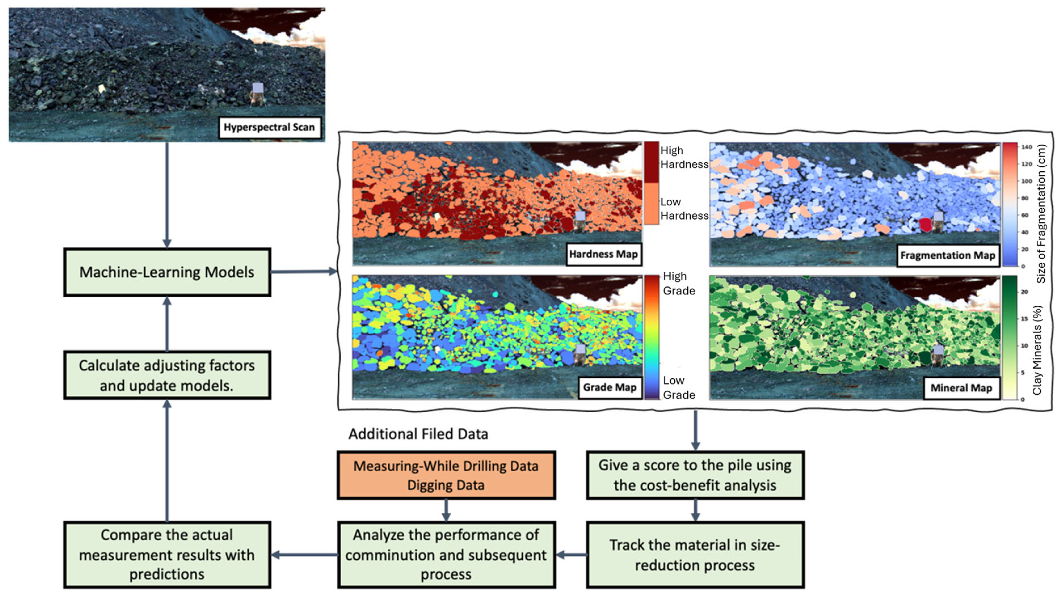
Figure 15 illustrates a conceptual workflow demonstrating the utilization of HSI for the optimization of comminution and subsequent processing. The process initiates with the scanning of a stockpile and the generation of maps of primary geometallurgical variables, which include hardness, grade, particle size distribution, and specific mineral identification. These outputs enable decision-makers to evaluate a given stockpile based on cost-benefit analyses, such as energy consumption during grinding or the suitability of the ore for specific processing routes. Subsequently, the material is tracked through the comminution and downstream processes, facilitating the ongoing assessment of actual performance against the model’s predictions. This assessment creates a feedback loop where any discrepancies prompt updates to the machine learning model and adjustments to various parameters, thereby continuously enhancing the predictive accuracy over time. Ultimately, by integrating the information obtained from HSI with supplementary field data, this workflow supports real-time decision-making: it helps operators optimize where and how to process different ore types and adjust milling and flotation parameters accordingly. Such an integrated system holds the potential for enhanced operational efficiency, reduced costs, and improved resource utilization throughout the mine-to-mill value chain.

It should be noted that the workflow presented in Figure 15 has not yet been piloted at the studied mine sites; rather, it represents a forward-looking conceptual framework informed by our results. Implementing HSI-driven decision-making in operational environments presents several practical challenges. These include the need for robust sensor deployment over large and dynamic stockpile surfaces, managing high data volumes and latency associated with hyperspectral acquisition, and integrating HSI outputs into existing mine-to-mill data systems. Additional barriers include ensuring consistent lighting conditions, developing on-site calibration routines, and aligning HSI data streams with production schedules. Despite these challenges, ongoing advancements in sensor technology, edge computing, and automated data processing continue to reduce these barriers, suggesting that operational deployment is increasingly feasible.

Recent research highlights a wide range of HIS applications in rock characterization in the field [70,71,72]. For instance, recent work by the authors has demonstrated the transferability of hyperspectral mineral mapping workflows from laboratory conditions to operational mine environments, including the scanning of muck piles at an open-pit mine [53]. The study showed that HSI-derived mineralogical information remains robust under field conditions and supports ore–waste discrimination at scales relevant to mining operations. These findings provide supporting evidence that the conceptual workflow illustrated in Figure 15 can be extended toward practical, cross-platform applications, even though full integration into mine planning systems was beyond the scope of the present study.

5. Conclusions

This study aimed to explore the potential application of several geochemical and geomechanical testing methods, including pXRF, LRH, CAI, and hyperspectral imaging, in characterizing the grindability behavior of ore during the comminution process. To do so, sixty-two rock samples were collected from two adjacent gold open-pit mines. After performing the specified geochemical and geomechanical testing methods, these samples were categorized based on their grade, abrasivity, and the classifications assigned by the on-site geologist, resulting in the formation of ten distinct ore groups. Subsequently, the BWI testing was utilized to assess the grinding characteristics of these ore groups, revealing that they are classified into two categories: moderate (<15 kWh/t) and hard materials (>15 kWh/t).

The results demonstrate that the mentioned testing methods can serve as viable proxies for characterizing ore grindability, each with its own practicality and resolution. HSI stands out for its capacity to collect spatially continuous mineralogical data, which is especially valuable in complex geological settings or large open pits. The findings indicate that particular spectral features—such as “Band Ratio 9” or the “frequency of absorption peak at 2336 nm”—can effectively discriminate between moderate and hard grindability classes. In addition, a conceptual workflow is discussed for incorporating HSI in the mine site and how it could be integrated with the other data sources to assist not only in comminution planning but also in flotation optimization.

Lastly, it is also worth noting that the primary objective of this study was to highlight and compare the potential applications of various geochemical and geomechanical testing methods in characterizing the grindability behavior of ore groups. It must also be noted that these analyses have been conducted on a limited number of BWI tests. Although promising results were found, more rock samples are needed not only to confirm the application of these approaches to characterizing the grinding behavior but also to develop a machine learning-based model for predicting the BWI value for different parts of the rock piles.

References

1. Lois-Morales, P.; Evans, C.; Weatherley, D. Quantifying the Relationship between Particles’ Strength and Their Mineralogical and Textural Characteristics. Miner. Eng. 2023, 199, 108113. [Google Scholar] [CrossRef] [Scilit]
2. Dominy, S.C.; O’connor, L.; Parbhakar-Fox, A.; Glass, H.J.; Purevgerel, S. Geometallurgy—A Route to More Resilient Mine Operations. Minerals 2018, 8, 560. [Google Scholar] [CrossRef] [Scilit]
3. Coward, S.; Vann, J.; Dunham, S.; Stewart, M. The Primary-Response Framework for Geometallurgical Variables. In Proceedings of the 7th International Mining Geology Conference, Perth, Australia, 17–19 August 2009; Dominy, S., Ed.; Australasian Institute of Mining and Metallurgy: Melbourne, Australia, 2009; pp. 109–113. [Google Scholar]
4. Sepulveda, E.; Dowd, P.A.; Xu, C.; Addo, E. Multivariate Modelling of Geometallurgical Variables by Projection Pursuit. Math. Geosci. 2017, 49, 121–143. [Google Scholar] [CrossRef] [Scilit]
5. Napier-Munn, T.J.; Morrell, S.; Morrison, R.D.; Kojovic, T. Mineral Comminution Circuits Their Operation and Optimization; Julius Kruttschnitt Mineral Research Centre, University of Queensland: Indooroopilly, Australia, 1996; ISBN 064628861X. [Google Scholar]
6. Morrell, S. A Global and Mining Industry Perspective of the Role of Comminution in the 1.5 °C Future. In Proceedings of the 2023 SME Annual Conference & Expo. SME, Denver, CO, USA, 26 February–1 March 2023. [Google Scholar]
7. Napier-Munn, T. Comminution Energy and How to Reduce It. In Proceedings of the 2012 CEEC Workshop, Noosa, Australia, 12–13 June 2012; CEEC: Beijing, China, 2012; p. 17. [Google Scholar]
8. Deniz, V.; Ozdag, H. A New Approach to Bond Grindability and Work Index: Dynamic Elastic Parameters. Miner. Eng. 2003, 16, 211–217. [Google Scholar] [CrossRef] [Scilit]
9. Bond, F.C. Crushing and Grinding Calculation Part I. Br. Chem. Eng. 1961, 6, 378–385. [Google Scholar]
10. Barbosa, P.d.A.; Bergerman, M.G.; da Fonseca, E.; Kwitko-Ribeiro, R. Determination of Abrasiveness in Copper-Gold Sulfide Ores: A Contribution to the Geometallurgical Model of the Sossego Deposit. Minerals 2021, 11, 1427. [Google Scholar] [CrossRef] [Scilit]
11. Guimarães Bergerman, M.; Pamparana, G.; Delboni, H.; Klein, B. Development of a Simplified Test for the Determination of the Bond Ball Mill Work Index Using a Modified Hardgrove Test. Miner. Eng. 2023, 203, 108359. [Google Scholar] [CrossRef] [Scilit]
12. Rodríguez-Torres, I.; Tuzcu, E.T.; Andrade-Martínez, J.; Rosales-Marín, G. Estimation Methodology for Bond Ball Mill Work Index Experiment Output via Mathematical Modeling. Miner. Eng. 2023, 201, 108186. [Google Scholar] [CrossRef] [Scilit]
13. Valerevich Lvov, V.; Sergeevich Chitalov, L. Comparison of the Different Ways of the Ball Bond Work Index Determining. Int. J. Mech. Eng. Technol. 2019, 10, 1180–1194. [Google Scholar]
14. Bhuiyan, M.; Esmaeili, K.; Ordóñez-Calderón, J.C. Evaluation of Rock Characterization Tests as Geometallurgical Predictors of Bond Work Index at the Tasiast Mine, Mauritania. Miner. Eng. 2022, 175, 107293. [Google Scholar] [CrossRef] [Scilit]
15. Todorovic, D.; Trumic, M.; Andric, L.; Milosevic, V.; Trumic, M. A Quick Method for Bond Work Index Approximate Value Determination. Physicochem. Probl. Miner. Process. 2016, 53, 321–332. [Google Scholar] [CrossRef] [Scilit]
16. Ford, E.; Sithole, V. A Comparison of Test Procedures for Estimating the Bond Ball Work Index on Zambian/DRC Copper–Cobalt Ores and Evaluation of Suitability for Use in Geometallurgical Studies. In Proceedings of the Copper Cobalt Africa, Incorporating the 8th Southern African Base Metals Conference, Livingstone, Zambia, 6 July 2015; pp. 65–68. [Google Scholar]
17. Ahmadi, R.; Shahsavari, S. Procedure for Determination of Ball Bond Work Index in the Commercial Operations. Miner. Eng. 2009, 22, 104–106. [Google Scholar] [CrossRef] [Scilit]
18. Magdalinovic, N.; Trumic, M.; Trumic, G.; Magdalinovic, S.; Trumic, M. Determination of the Bond Work Index on Samples of Non-Standard Size. Int. J. Miner. Process. 2012, 114–117, 48–50. [Google Scholar] [CrossRef] [Scilit]
19. Nikolić, V.; Trumić, M. A New Approach to the Calculation of Bond Work Index for Finer Samples. Miner. Eng. 2021, 165, 106858. [Google Scholar] [CrossRef] [Scilit]
20. Nikolić, V.; Doll, A.; Trumić, M. A New Methodology to Obtain a Corrected Bond Ball Mill Work Index Valid with Non-Standard Feed Size. Miner. Eng. 2022, 188, 107822. [Google Scholar] [CrossRef] [Scilit]
21. Ozkahraman, H.T. A Meaningful Expression between Bond Work Index, Grindability Index and Friability Value. Miner. Eng. 2005, 18, 1057–1059. [Google Scholar] [CrossRef] [Scilit]
22. Swain, R.; Rao, R.B. Alternative Approaches for Determination of Bond Work Index on Soft and Friable Partially Laterised Khondalite Rocks of Bauxite Mine Waste Materials. J. Miner. Mater. Charact. Eng. 2009, 8, 729–743. [Google Scholar] [CrossRef]
23. Montoya, P.; Keeney, L.; Jahoda, R.; Hunt, J.; Berry, R.; Drew, U.; Chamberlain, V.; Leichliter, S. Geometallurgical Modelling Techniques Applicable to Prefeasibility Projects—La Colosa Case Study. In Proceedings of the First AusIMM International Geometallurgy Conference, Brisbane, Australia, 5–7 September 2011; Dominy, S., Ed.; AusIMM: Melbourne, Australia, 2011; pp. 103–111. [Google Scholar]
24. Gent, M.; Menendez, M.; Toraño, J.; Torno, S. A Correlation between Vickers Hardness Indentation Values and the Bond Work Index for the Grinding of Brittle Minerals. Powder Technol. 2012, 224, 217–222. [Google Scholar] [CrossRef] [Scilit]
25. Haffez, G.S.A. Correlation between Work Index and Mechanical Properties of Some Saudi Ores. Mater. Test. 2012, 54, 108–112. [Google Scholar] [CrossRef] [Scilit]
26. Harbort, G.J.; Lam, K.; Sola, C. The Use of Geometallurgy to Estimate Comminution Parameters within Porphyry Copper Deposits. In Proceedings of the Second AusIMM International Geometallurgy Conference, Brisbane, Australia, 30 September–2 October 2013; pp. 217–230. [Google Scholar]
27. Hunt, J.; Kojovic, T.; Berry, R. Estimating Comminution Indices from Ore Mineralogy, Chemistry and Drill Core Logging. In Proceedings of the Second AusIMM International Geometallurgy Conference, Brisbane, Australia, 30 September–2 October 2013; Dominy, S., Ed.; The Australasian Institute of Mining and Metallurgy (AusIMM): Carlton, Australia, 2013. [Google Scholar]
28. Chandar, K.R.; Deo, S.N.; Baliga, A.J. Prediction of Bond’s Work Index from Field Measurable Rock Properties. Int. J. Miner. Process 2016, 157, 134–144. [Google Scholar] [CrossRef] [Scilit]
29. van Duijvenbode, J.R.; Cloete, L.M.; Shishvan, M.S.; Buxton, M.W.N. Material Fingerprinting as a Tool to Investigate between and within Material Type Variability with a Focus on Material Hardness. Miner. Eng. 2022, 189, 107885. [Google Scholar] [CrossRef] [Scilit]
30. Both, C.; Dimitrakopoulos, R. Integrating Geometallurgical Ball Mill Throughput Predictions into Short-Term Stochastic Production Scheduling in Mining Complexes. Int. J. Min. Sci. Technol. 2023, 33, 185–199. [Google Scholar] [CrossRef] [Scilit]
31. Ghadernejad, S.; Esmaeili, K. Investigating the Relationship Between Geochemistry, Leeb Rebound Hardness, and Cerchar Abrasivity Index. Int. J. Geomech. 2024, 24, 04024280. [Google Scholar] [CrossRef] [Scilit]
32. Crosera, M.; Baracchini, E.; Prenesti, E.; Giacomello, A.; Callegher, B.; Oliveri, P.; Adami, G. Elemental Characterization of Surface and Bulk of Copper-Based Coins from the Byzantine-Period by Means of Spectroscopic Techniques. Microchem. J. 2019, 147, 422–428. [Google Scholar] [CrossRef] [Scilit]
33. Pavoni, E.; Crosera, M.; Petranich, E.; Adami, G.; Faganeli, J.; Covelli, S. Partitioning and Mixing Behaviour of Trace Elements at the Isonzo/Soča River Mouth (Gulf of Trieste, Northern Adriatic Sea). Mar. Chem. 2020, 223, 103800. [Google Scholar] [CrossRef] [Scilit]
34. Sibilia, M.; Stani, C.; Gigli, L.; Pollastri, S.; Migliori, A.; D’Amico, F.; Schmid, C.; Licen, S.; Crosera, M.; Adami, G.; et al. A Multidisciplinary Study Unveils the Nature of a Roman Ink of the I Century AD. Sci. Rep. 2021, 11, 7231. [Google Scholar] [CrossRef] [Scilit]
35. Leeb, D. Dynamic Hardness Testing of Metallic Materials. NDT Int. 1979, 12, 274–278. [Google Scholar] [CrossRef] [Scilit]
36. Proceq, S.A. Equotip 3 Portable Hardness Tester, Operating Instructions; Proceq SA: Schwerzenbach, Switzerland, 2007. [Google Scholar]
37. Desarnaud, J.; Kiriyama, K.; Bicer Simsir, B.; Wilhelm, K.; Viles, H. A Laboratory Study of Equotip Surface Hardness Measurements on a Range of Sandstones: What Influences the Values and What Do They Mean? Earth Surf. Process Landf. 2019, 44, 1419–1429. [Google Scholar] [CrossRef] [Scilit]
38. Alber, M. Stress Dependency of the Cerchar Abrasivity Index (CAI) and Its Effects on Wear of Selected Rock Cutting Tools. Tunn. Undergr. Space Technol. 2008, 23, 351–359. [Google Scholar] [CrossRef] [Scilit]
39. Plinninger, R.; Kasling, H.; Thuro, K. Wear Prediction in Hardrock Excavation Using the CERCHAR Abrasiveness Index (CAI). In Proceedings of the Eurock 2004 and 53rd Geomechanics Colloquium, Salzburg, Austria, 7–9 October 2004; pp. 599–604. [Google Scholar]
40. Rostami, J.; Ghasemi, A.; Alavi Gharahbagh, E.; Dogruoz, C.; Dahl, F. Study of Dominant Factors Affecting Cerchar Abrasivity Index. Rock. Mech. Rock. Eng. 2014, 47, 1905–1919. [Google Scholar] [CrossRef] [Scilit]
41. Alber, M.; Yaralı, O.; Dahl, F.; Bruland, A.; Käsling, H.; Michalakopoulos, T.N.; Cardu, M.; Hagan, P.; Aydın, H. ISRM Suggested Method. for Determining the Abrasivity of Rock. by the CERCHAR Abrasivity Test. Rock. Mech. Rock. Eng. 2013, 47, 261–266. [Google Scholar] [CrossRef] [Scilit]
42. Yang, B.; Wang, S.; Li, S.; Zhou, B.; Zhao, F.; Ali, F.; He, H. Research and Application of UAV-Based Hyperspectral Remote Sensing for Smart City Construction. Cogn. Robot. 2022, 2, 255–266. [Google Scholar] [CrossRef] [Scilit]
43. Schaefer, L.N.; Kereszturi, G.; Villeneuve, M.; Kennedy, B. Determining Physical and Mechanical Volcanic Rock Properties via Reflectance Spectroscopy. J. Volcanol. Geotherm. Res. 2021, 420, 107393. [Google Scholar] [CrossRef] [Scilit]
44. Schaefer, L.N.; Kereszturi, G.; Kennedy, B.M.; Villeneuve, M. Characterizing Lithological, Weathering, and Hydrothermal Alteration Influences on Volcanic Rock Properties via Spectroscopy and Laboratory Testing: A Case Study of Mount Ruapehu Volcano, New Zealand. Bull. Volcanol. 2023, 85, 43. [Google Scholar] [CrossRef] [Scilit]
45. Kereszturi, G.; Heap, M.; Schaefer, L.N.; Darmawan, H.; Deegan, F.M.; Kennedy, B.; Komorowski, J.C.; Mead, S.; Rosas-Carbajal, M.; Ryan, A.; et al. Porosity, Strength, and Alteration—Towards a New Volcano Stability Assessment Tool Using VNIR-SWIR Reflectance Spectroscopy. Earth Planet. Sci. Lett. 2023, 602, 117929. [Google Scholar] [CrossRef] [Scilit]
46. Lee, S.J.; Jeong, G.C.; Kim, J.T. Analysis and Comparison of Rock Spectroscopic Information Using Drone-Based Hyperspectral Sensor. J. Eng. Geol. 2021, 31, 479–492. [Google Scholar] [CrossRef]
47. Bakun-Mazor, D.; Ben-Ari, Y.; Notesko, G.; Marco, S.; Ben-Dor, E. Measuring Carbonate Rock Strength Using Spectroscopy across the Optical and Thermal Region. IOP Conf. Ser. Earth Environ. Sci. 2021, 833, 012025. [Google Scholar] [CrossRef] [Scilit]
48. Okada, N.; Maekawa, Y.; Owada, N.; Haga, K.; Shibayama, A.; Kawamura, Y. Automated Identification of Mineral Types and Grain Size Using Hyperspectral Imaging and Deep Learning for Mineral Processing. Minerals 2020, 10, 809. [Google Scholar] [CrossRef] [Scilit]
49. Maras, E.E.; Caniberk, M.; Odabas, M.S.; Degerli, B.; Maras, S.S.; Maras, H.H. An Evaluation of the Relationship between Physical/Mechanical Properties and Mineralogy of Landscape Rocks as Determined by Hyperspectral Reflectance. Arab. J. Geosci. 2016, 9, 164. [Google Scholar] [CrossRef] [Scilit]
50. Ghadernejad, S.; Esmaeili, K. Predicting Rock Hardness and Abrasivity Using Hyperspectral Imaging Data and Random Forest Regressor Model. Remote Sens. 2024, 16, 3778. [Google Scholar] [CrossRef] [Scilit]
51. Akbar, S.; Abdolmaleki, M.; Ghadernejad, S.; Esmaeili, K. Applying Knowledge-Based and Data-Driven Methods to Improve Ore Grade Control of Blast Hole Drill Cuttings Using Hyperspectral Imaging. Remote Sens. 2024, 16, 2823. [Google Scholar] [CrossRef] [Scilit]
52. Ghadernejad, S.; Esmaeili, K.; Consens, M.P. Sensor-Based Rock Hardness Characterization in a Gold Mine Using Hyperspectral Imaging and Portable X-Ray Fluorescence Technologies. Remote Sens. 2025, 17, 2062. [Google Scholar] [CrossRef] [Scilit]
53. Abdolmaleki, M.; Ghadernejad, S.; Esmaeili, K. Automated Hyperspectral Ore–Waste Discrimination for a Gold Mine: Comparative Study of Data-Driven and Knowledge-Based Approaches in Laboratory and Field Environments. Minerals 2025, 15, 741. [Google Scholar] [CrossRef] [Scilit]
54. HySpex HySpex Mjolnir VS-620 Configuration. Available online: https://www.hyspex.com/hyspex-products/hyspex-mjolnir/hyspex-mjolnir-vs-620/ (accessed on 19 May 2024).
55. ASTM A956; Standard Test Method for Leeb Hardness Testing of Steel Products. ASTM International: West Conshohocken, PA, USA, 2017. [CrossRef] [Scilit]
56. Ghadernejad, S.; Esmaeili, K. The Application of Small Sample Theory and Confidence Interval Method to Determine the Representative Mean Leeb Rebound Hardness Value. Bull. Eng. Geol. Environ. 2024, 83, 25. [Google Scholar] [CrossRef] [Scilit]
57. Kadachi, A.N.; Al-Eshaikh, M.A. Limits of Detection in XRF Spectroscopy. X-Ray Spectrom. 2012, 41, 350–354. [Google Scholar] [CrossRef] [Scilit]
58. EPA SW-846; Test Method 6200: Field Portable X-Ray Fluorescence Spectrometry for the Determination of Elemental Concentrations in Soil and Sediment. United States Environmental Protection Agency: Washington, DC, USA, 2007.
59. Mann, H.B.; Whitney, D.R. On a Test of Whether One of Two Random Variables Is Stochastically Larger than the Other. Ann. Math. Stat. 1947, 18, 50–60. [Google Scholar] [CrossRef] [Scilit]
60. Hollander, M.; Wolfe, D.A.; Chicken, E. Nonparametric Statistical Methods; Wiley: Hoboken, NJ, USA, 2015; ISBN 9781119196037. [Google Scholar]
61. Conover, W.J. Practical Nonparametric Statistics, 3rd ed.; John Wiley & Sons: Hoboken, NJ, USA, 1999; Volume II, ISBN 978-0-471-16068-7. [Google Scholar]
62. Sheskin, D.J. Handbook of Parametric and Nonparametric Statistical Procedures, 5th ed.; Chapman and Hall/CRC: Boca Raton, FL, USA, 2020; ISBN 9780429186196. [Google Scholar]
63. Smirnov, N. Table for Estimating the Goodness of Fit of Empirical Distributions. Ann. Math. Stat. 1948, 19, 279–281. [Google Scholar] [CrossRef] [Scilit]
64. Massey, F.J. The Kolmogorov-Smirnov Test for Goodness of Fit. J. Am. Stat. Assoc. 1951, 46, 68. [Google Scholar] [CrossRef]
65. Gibbons, J.D.; Chakraborti, S. Nonparametric Statistical Inference; Chapman and Hall/CRC: New York, NY, USA, 2010. [Google Scholar] [CrossRef] [Scilit]
66. Yang, K.; Browne, P.R.L.; Huntington, J.F.; Walshe, J.L. Characterising the Hydrothermal Alteration of the Broadlands–Ohaaki Geothermal System, New Zealand, Using Short-Wave Infrared Spectroscopy. J. Volcanol. Geotherm. Res. 2001, 106, 53–65. [Google Scholar] [CrossRef] [Scilit]
67. Lang, H.; Botha, R.; Hume, K.; Sandler, S.; Haest, M. MineSense Technology Empowering Bucket Resolution Mine to Mill Reconciliation. In Proceedings of the International Mining Geology Conference, Brisbane, QLD, Australia, 22–23 March 2022. [Google Scholar]
68. Chen, X.; Peng, Y. Managing Clay Minerals in Froth Flotation—A Critical Review. Miner. Process. Extr. Metall. Rev. 2018, 39, 289–307. [Google Scholar] [CrossRef] [Scilit]
69. Toro, N.; Ghorbani, Y.; Turan, M.D.; Robles, P.; Gálvez, E. Gangues and Clays Minerals as Rate-Limiting Factors in Copper Heap Leaching: A Review. Metals 2021, 11, 1539. [Google Scholar] [CrossRef] [Scilit]
70. Koerting, F.; Asadzadeh, S.; Hildebrand, J.C.; Savinova, E.; Kouzeli, E.; Nikolakopoulos, K.; Lindblom, D.; Koellner, N.; Buckley, S.J.; Lehman, M.; et al. VNIR-SWIR Imaging Spectroscopy for Mining: Insights for Hyper-spectral Drone Applications. Mining 2024, 4, 1013–1057. [Google Scholar] [CrossRef] [Scilit]
71. Jingping, H.; Barton, I. Hyperspectral remote sensing for detecting geotechnical problems at Ray mine. Eng. Geol. 2021, 292, 106261. [Google Scholar] [CrossRef] [Scilit]
72. Barton, I.; Gabriel, M.J.; Lyons-Baral, J.; Barton, M.D.; Duplessis, L.; Roberts, C. Extending geometallurgy to the mine scale with hyperspectral imaging: A pilot study using drone- and ground-based scanning. Min. Metall. Explor. 2021, 38, 799–818. [Google Scholar] [CrossRef] [Scilit]
Figure 1. Data collection steps: (a) pXRF device, (b) hyperspectral imaging system, (c) LRH test, (d) CAI test, and (e) BWI test.
Minerals 16 00115 g001
Figure 2. The distribution and statistical summary of the measured representative mean HLD values of the collected rock samples.
Minerals 16 00115 g002
Figure 3. The distribution and statistical summary of the measured mean CAI values of the collected rock samples.
Minerals 16 00115 g003
Figure 4. The preprocessing steps of hyperspectral Imaging data: (a) raw SWIR image, (b) Radiometric corrected SWIR image (false color at R: 1650 nm, G: 1072 nm, B: 1026 nm), (c) comparison between DN and reflectance for the same spot before and after radiometric correction, (d) the dimension of the radiometric corrected SWIR before cropping, (e) the dimension of the radiometric corrected SWIR after cropping, and (f) comparison between the background pixel spectrum for the same spot before and after background pixel removal.
Minerals 16 00115 g004
Figure 5. The true color illustration of all 62 rock samples grouped in ten ore groups used for the BWI test.
Minerals 16 00115 g005
Figure 6. The process and results of the spectral feature extraction, (a) the obtained optimal cluster number using the elbow method, (b) the visualization of the dominant spectral curves obtained from clustering analysis, and (c) the feature extraction process on the dominant spectral curves obtained from the clustering analysis.
Minerals 16 00115 g006
Figure 7. The absorption-peak-based feature extraction method includes: (a) the graphical representation of the hyperspectral image, (b) a 3D matrix representation of the hyperspectral image, (c) a 2D matrix representation of the hyperspectral image (a spectrum for each cell), (d) the graphical representation of a spectrum, (e) the application of continuum removal and the absorption peak procedure for a single spectrum from the hyperspectral image, (f) the application of this method for all pixels, and (g) the results of the absorption peak for a rock sample presented in table form.
Minerals 16 00115 g007
Figure 8. The relationship between BWI classes and (a) mean HLD and (b) CAI values.
Minerals 16 00115 g008
Figure 9. The comparison of mean geochemical feature values across BWI classes.
Minerals 16 00115 g009
Figure 10. The comparison of the band ratio-based spectral features across different grindability behaviors.
Minerals 16 00115 g010
Figure 11. The comparison of the absorption-based spectral features across different grindability behaviors.
Minerals 16 00115 g011
Figure 12. The distribution of some of the geochemical features in the two studied pits.
Minerals 16 00115 g012
Figure 13. The observed contact zones in Pit 2.
Minerals 16 00115 g013
Figure 14. The distribution of different rock types at the stockpile sourced from a complex geological area after blasting.
Minerals 16 00115 g014
Figure 15. A conceptual workflow for incorporating hyperspectral imaging in the mine site.
Minerals 16 00115 g015