Classification of Thin-Section Rock Images Using a Combined CNN and SVM Approach

Abstract

The accurate classification of rocks is crucial for applications such as earthquake prediction, resource exploration, and geological analysis. Traditional methods rely on expert examination of thin-section images under a microscope, making the process time-consuming and prone to errors. Recent advancements in deep learning have emerged as a powerful tool for automated rock classification; however, distinguishing between similar rock types such as sedimentary, metamorphic, and magmatic rocks remains a challenge. This study proposes a novel hybrid convolutional neural network (CNN) approach that combines the strengths of VGG16 and EfficientNetV2 architectures for the classification of thin-section rock images. The model, developed using the Feature-Selected Hybrid Network (FSHNet), demonstrates significant improvements over individual models, achieving a 5% increase in accuracy compared to Efficient-NetV2B0 and a 9% increase compared to VGG16. By employing the ReliefF algorithm for feature selection and Support Vector Machines (SVMs) for classification, the model further reduces the dimensionality of the feature space, enhancing computational efficiency. The proposed model has been applied to two different rock datasets. The first dataset consists of 2634 images, categorized into sedimentary, metamorphic, and magmatic rock classes. Additionally, the approach was tested on a second dataset comprising petrographic microfacies images, demonstrating its effectiveness in multiclass geological structure classification. Validation on both datasets shows that the proposed method outperforms popular deep learning models and previous studies, achieving a 3% increase in accuracy. These results highlight that the proposed approach provides a robust and efficient solution for automated rock classification, offering significant advancements for geological research and real-world applications.

1. Introduction

Engineering solutions to natural disasters have gained increasing importance in recent years. Natural disasters involving geological phenomena are complex events that encompass rock types, tectonism, and processes occurring within the Earth’s crust. The crust, composed of igneous, sedimentary, and metamorphic rocks, can be understood through the interpretation of rocks with different compositions and properties [1]. Rock classification is a time-consuming process that requires expert analysis using various methods such as macroscopic observation, microscopic examination, or chemical analysis. Among these, thin-section analysis under polarized light microscopy is the most commonly used method, enabling the identification of mineral and rock types. The rocks in the dataset are difficult to distinguish because they typically contain multiple minerals. Previous studies have mostly focused on classifying rock types (igneous, sedimentary, or metamorphic) without explicitly utilizing the microscopic features of the minerals [2]. This study aims to identify both rock types and the key diagnostic properties of minerals (e.g., mineral shapes, cleavage, and/or twinning characteristics) from thin-section images (PPL—plane-polarized light and XPL—cross-polarized light).

Various imaging techniques, including polarized light microscopy, scanning electron microscopy, and energy dispersive X-ray spectroscopy, are employed for visualizing distinct minerals within rocks. The most commonly used of these techniques is polarized light microscopy. Identification and classification of rocks can be performed automatically with developments in the field of artificial intelligence in recent years. Machine learning in geology is used for the classification and segmentation of rocks and minerals, as well as for extracting mineral properties. In this study, a superpixel-based segmentation method was proposed for the segmentation of thin-section images [3]. This method aims to simplify the labeling process, which is particularly challenging in rock type classification based on semantic segmentation. For microfacies classification, a convolutional neural network-based transfer learning approach was proposed [4]. Mineral identification was performed on images obtained from thin-section rock samples. Additionally, five different microfacies rock types were classified. During the classification phase, VGG19, MobileNetv2, InceptionV3, and ResNet50 were utilized. In the deep learning-based classification of sedimentary rocks, an explainable artificial intelligence (XAI)-based model was used [5]. In this architecture, one of the networks analyzes a small portion of the image, while the other is capable of evaluating the entire image. For rock types with different origins, studies exist where VGG16 and GoogleNet were used with optimization models [6]. In a study involving thin-section rock images, it was observed that the use of online transfer learning-based feature mapping accelerated the training process [7]. In another study, a combined convolutional neural network was proposed for rock classification [8]. In another study, images captured under polarized and cross-polarized light were pre-processed, followed by the application of the principal component analysis (PCA) method. In this study, three convolutional neural networks with identical architectures achieved a success rate of 98.97% in classifying 13 rock types [9]. In a comparative analysis of ResNet18 and ResNet50 models for classifying petrographic thin-section images [4], it was observed that convolutional neural network models pre-trained with ImageNet performed better than models with randomly initialized weights, particularly in classes with similar features. In this study, the mineral dimensions in the thin-section images enabled the determination of rock type through petrographic image analysis. In the literature, studies that apply deep learning approaches to classify various rock types have mostly focused on fine-tuning popular deep learning models. For example, a deep learning-based segmentation approach has been proposed for sandstone classification [10]. This approach separates thin-section images into grain and background segments and primarily employs an encoder/decoder architecture. In many convolutional neural network models, attention modules, combinations of different models, and modified convolutional layers have been utilized. In a study that used a combined convolutional neural network model for rock classification, a complex classification approach was presented by integrating three different convolutional neural networks and applying techniques such as principal component analysis [10]. In one study, Li [11] combined rock texture images with image segmentation analysis methods to perform rock classification. In another study, Ishikawa [12] developed an automatic mineral classifier to identify certain igneous rocks. Cheng [13] aimed to automatically detect porosity in rocks. Yesiloglu-Gultekin [14] determined the percentage ratios of minerals in granite rocks. Baykan [15] identified mineral types from thin sections using the least squares error method. Singh [16] automatically characterized the surface texture of rocks using a multilayer perceptron neural network, based on 27 features extracted from 300 basalt rock samples collected from 90 different regions. Another researcher who used an SVM-based classification approach for rock texture classification was Shang [17], who applied both supervised and unsupervised feature selection methods to reduce classification complexity. In geological studies, dimensionality reduction approaches utilize important machine learning techniques such as Naive Bayes (NB), K-nearest neighbors (KNN), multilayer perceptron (MLP), random forest (RF), and support vector machine (SVM) [18,19]. Among these methods, RF, Naive Bayes, and KNN have demonstrated high accuracy in rock thin-section images and geological mapping [20]. SVM, employed for the automatic detection and classification of carbonate minerals, has shown particularly high accuracy [21,22]. For mineral recognition and classification, Yu et al. [23] applied a superpixel-based segmentation method to thin-section images. De Liama and Duarte [4] utilized a CNN-based transfer learning method for microfacies classification, Li et al. [24] employed a Grad-CAM-based inference method to classify rocks according to their origin, and Wang et al. [9] used an online transfer learning-based approach for the classification of thin-section rock images. Although SVM-based methods show promise in mineral classification, their performance improves when integrated with CNN-based deep learning techniques [25,26]. While CNNs excel at feature extraction, SVMs provide high robustness in classification. In this study, a hybrid model combining CNN and SVM was developed to identify mineral types.

The proposed approach consists of two stages. First, the outputs of the VGG16 and EfficientNetV2B0 base models are combined. Specifically, 512 features from VGG16 and 1280 features from EfficientNetV2B0 are merged. Then, average pooling, a dense layer, and a Softmax layer are added to form the final model. In the second stage, feature selection is performed on the total of 1792 combined features using the ReliefF algorithm, followed by classification with SVMs. The model’s accuracy is validated through five-fold cross-validation during the classification of the selected features with SVMs. The rocks in the dataset used are challenging to distinguish because they commonly contain minerals from other rock types.

2. Materials and Methods

2.1. Dataset of Rock Thin Sections

The dataset presented in this study includes igneous, metamorphic, and sedimentary rock types. Metamorphic rocks, formed under the influence of Earth’s internal forces, mainly contain quartz and plagioclase minerals, along with common metamorphic minerals such as garnet, kyanite, and sericite. Sedimentary rocks, formed by external forces, include quartz as well as secondary minerals like dolomite, calcite, and kaolinite. Igneous rocks, formed under the influence of internal forces, consist of primary minerals such as quartz, alkali feldspar, and plagioclase, and contain a greater variety and complexity of minerals, including quartz, feldspar, pyroxene, olivine, biotite, amphibole, and others. The classification encompasses igneous, sedimentary, and metamorphic rock types and considers minerals based on microscopic parameters such as color, shape, size, and cleavage. As shown in

Table 1. Number of thin-section images used in the dataset.

Rock Type	Number of Images
Igneous	963
Metamorphic	972
Sedimentary	699

, the dataset includes main rock groups (sedimentary, igneous, and metamorphic) as well as specific rock types within each group (e.g., limestone and sandstone as sedimentary rocks, granite as an igneous rock, and schist and gneiss as metamorphic rocks). Thin sections of selected rock types from sedimentary, igneous, and metamorphic groups were imaged under a polarizing microscope, and both plane-polarized light (PPL) and cross-polarized light (XPL) images are presented in Figure 1. A total of 2634 thin-section images representing 105 rock types were acquired at a resolution of 1280 × 1024 pixels. These images include views obtained in both PPL and XPL modes of the polarizing microscope. The aim is to use PPL images to distinguish minerals that appear similar in color under XPL by considering properties such as cleavage or pleochroic color (Figure 1). Ultimately, mineral identification with maximum accuracy is achieved based on distinguishing characteristics (e.g., color, shape, grain size, cleavage, pleochroism), and the rock group is determined according to its mineralogical composition. The images employed in this study were obtained from the Nanjing University photomicrograph dataset for petrology teaching, as described by Wei et al. [27].

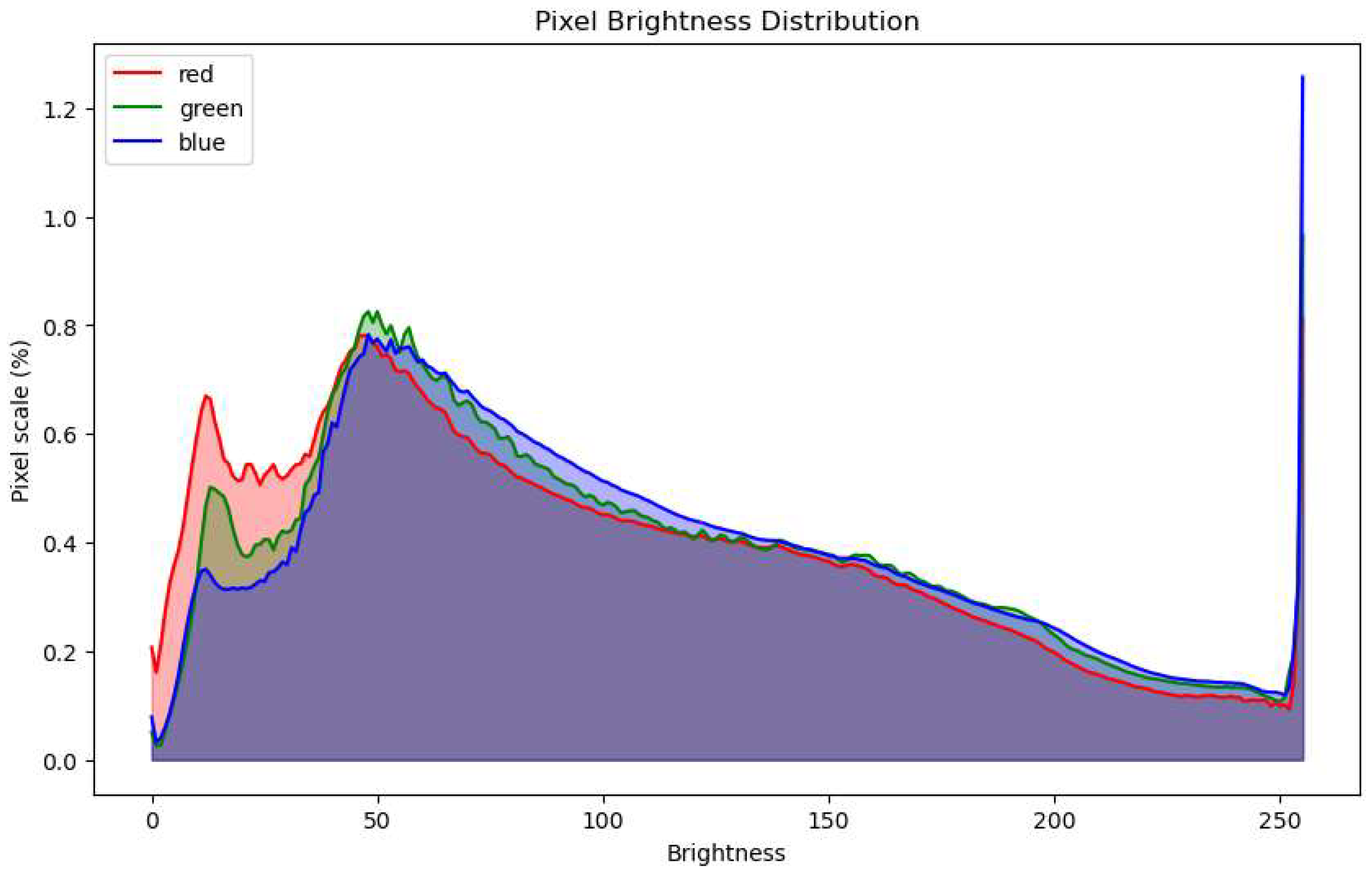
The high-resolution thin section images, acquired in JPG format, are named according to the convention “section position” + “rock name” + “section serial number.” The number of thin-section images for each rock group is presented in Table 1. The dataset includes 40 sub-classes of metamorphic rocks, 28 sub-classes of sedimentary rocks, and 40 sub-classes of igneous rocks. Thin-section images were obtained under both cross-polarized and plane-polarized light. A thin-section image of a metamorphic rock is shown in Figure 1a, while pixel brightness distribution for all rock groups in the dataset is presented in Figure 1. The variation in color and brightness distribution in cross-sectional images is shown (Figure 2).

2.2. EfficientNetv2 Model

EfficientNetv2 is a deep neural network architecture proposed to address the shortcomings of the previous EfficientNet model [28] (Figure 3).

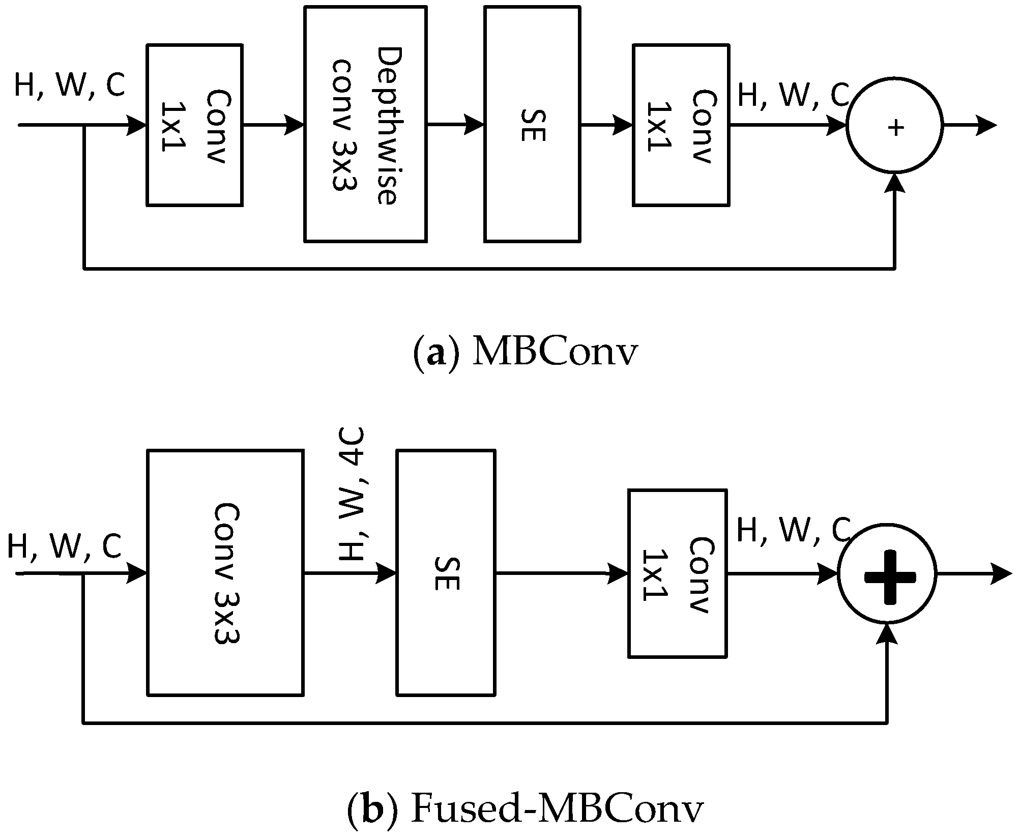
The most distinctive feature of the EfficientNetv2 architecture is the use of Fused-MBConv convolutional blocks. These blocks are utilized in the initial layers of the network, followed by MBConv blocks from the original EfficientNet architecture (Figure 4). Although Fused-MBConv blocks slightly increase the number of parameters, they accelerate the training process.

2.3. VGG16 Model

VGG16 is one of the most effective architectures for computer vision applications and has the capability to extract features for tasks such as classification and regression [29]. This model uses color or grayscale images with dimensions of 224 × 224 × 3 (Figure 5). Despite its considerable depth, this model requires more computational resources compared to modern deep learning architectures. The simple yet powerful architecture of VGG16 facilitates the learning process and enables effective results on large datasets.

2.4. The Proposed Hybrid Model

The proposed method integrates the EfficientNetV2 model, which is characterized by a low number of parameters, with VGG16, a robust classification approach. The structure of the VGG16 model enables extraction of mineral edges, textures, and fundamental patterns from thin-section rock images. Its early and mid-level convolutional layers are particularly effective in distinguishing microstructural differences among rock types. EfficientNetV2, as a parameter-efficient network, is capable of learning complex features with lower computational cost. Through integration of these two models, mineral types can be distinguished, thereby enabling accurate rock classification. To prevent the model from memorizing only specific features, the ReliefF algorithm is employed. This algorithm selects the most significant features, which helps reduce risk of overfitting and ensures more accurate predictions. The proposed method consists of two stages. In the first stage, the 7 × 7 × 512 features extracted from the maxpooling_2d_5 layer of the VGG16 model are combined with the 8 × 8 × 1280 features obtained from the top activation layer of the EfficientNetV2 model, following average pooling. In the second stage, the 7 × 7 × 512 feature maps are extracted from the MaxPooling2D_5 layer of VGG16 model. Due to differences in feature map dimensions, an average pooling layer is applied to ensure dimensional compatibility between the extracted features, reduce the risk of overfitting in small datasets, and preserve the most salient features. These feature maps capture the unique mineral compositions and textural differences of various rock types, enhancing the model’s ability to distinguish between similar rock classes. While the early and mid-level convolutional layers of the VGG16 model primarily extract edges, textures, and fundamental patterns, the MaxPooling2D_5 layer captures high-level features. By combining the 7 × 7 × 512 feature space obtained from VGG16 with EfficientNetV2B0, the rock classification capability is significantly improved. This fusion is highly effective in identifying differences between rock types. After the dense layer, rock types are classified through a Softmax layer. Among the approximately 1792 features, the most relevant ones are selected using the ReliefF algorithm. These selected features are then fed into Support Vector Machines (SVMs) for classification (Figure 6). As shown in Figure 6, the proposed hybrid architecture integrates feature extraction capabilities while employing a fine-tuning approach to enhance classification performance. In the fine-tuning process, the final convolutional layers of both models were unfrozen and retrained using the dataset. This allowed networks to refine their learned feature representations for geological analysis. Through fine-tuning, the models were enabled to capture domain-specific features that are critical in thin-section rock classification.

2.5. FSHNet

To enhance and gain significant memory gains, we selected to deploy feature selection techniques. With this kind of approach, learned features during the training process can be used, while heavy classification heads can be changed by the much more efficient SVM classifier using the ReliefF algorithm. After the feature merging process, feature selection was performed using the ReliefF algorithm, eliminating irrelevant features. By employing SVMs for classification, higher accuracy was achieved using a reduced number of features.

Support Vector Machines (SVMs) [30], which are binary classification methods that aim to find the optimal hyperplane that separates the data into two distinct classes, define a decision boundary that maximizes the margin between the loosest data points of each class (support vectors). This margin contributes to the model’s ability to generalize to new data and enhances its robustness against minor variations, thereby reducing risk of overfitting. In this study, after feature selection, five-fold cross-validation was employed using performance metrics such as accuracy, precision, recall, and F1-score to accurately evaluate the performance of the SVM classifier and enhance its generalization capability. To optimize the hyperparameters of the SVM, the grid search method was combined with five-fold cross-validation. For each hyperparameter set, the model was trained and validated five times, and the average performance metric was calculated. The hyperparameter set that yielded the best cross-validation performance was selected as the final model configuration. Through an exhaustive search of the hyperparameter space and the use of cross-validation, the model was not only optimized for training data but also configured to generalize effectively to unseen data. The ReliefF algorithm is an extension of the Relief algorithm developed for feature selection [31]. It evaluates the quality of features based on how effectively they distinguish between neighboring instances. It is particularly effective for problems involving noisy data and redundant features [32]. ReliefF ranks features according to their importance and identifies those that contribute most significantly to classification (Algorithm 1). Additionally, features that exhibit low variability among instances within the same class are assigned higher importance scores. This approach helps retain relevant and discriminative features while eliminating redundant or irrelevant ones. By reducing the number of features, classification models can operate on smaller but more meaningful datasets, thereby lowering computational costs. Moreover, removing unnecessary features improves the overall classification performance.

Algorithm 1 Relief Feature Selection Algorithm

Require: Dataset X with m instances and n features, class labels Y

Ensure: Feature weights W representing feature importance 1: Initialize all feature weights W[j] = 0 for j = 1,2,…,n 2: for i = 1 to m do 3:   Find nearest neighbors: 4:   Nhit = nearest instance to i with the same class label 5:   Nmisst = nearest instance to i with different class label 6:   for j = 1 to n do 7:     W[j] = W[j] − ∣xi,j − xNhit,j∣/m + ∣xi,j − xN miss,j∣/m 8:   end for 9: end for 10: Normalize weights W to range [0, 1] 11: Rank features based on weights W 12: return W

3. Evaluation Metrics

The performance of the proposed approach is evaluated on certain metrics. These metrics measure how well the model’s predictions match the actual values. Commonly used metrics for classification problems include accuracy, precision, recall, and F1 score. These metrics are calculated from the confusion matrix. The accuracy measures the proportion of instances that the model correctly classifies. The accuracy can be a good metric when all the classes are equally important. This metric is given in (1).

$$Accuracy={\displaystyle \frac{Correctlyclassifiedsamples}{Allsampes}}$$

(1)

Precision measures the proportion of samples predicted as positive that are truly positive. Precision is crucial when the cost of false positive predictions is high. The precision metric is measured via (2) the following equation:

$$Precision={\displaystyle \frac{TP}{TP+FP}}$$

(2)

In (2), TP and FP represent the true positive and false positive rates, respectively. Recall measures the proportion of truly positive samples that are accurately predicted. Recall is crucial when the cost of false negative predictions is high. The recall metric is given in (3).

$$Recall={\displaystyle \frac{TP}{TP+FN}}$$

(3)

In (3), the FN value represents the false negative rate. The F1-score measures the trade-off between precision and recall. The F1-score balances the impact of both false positive predictions and false negative predictions of the model. This metric is given in (4).

$$F1=2\times {\displaystyle \frac{Precision\times Recall}{Precision+Recall}}$$

(4)

In addition to accuracy, other metrics were used to evaluate the results of the application.

4. Results

In this study, which aimed to classify different types of rocks using rock thin sections—crucial tools in the interpretation of geological data—various learning rates were tested for each rock type, and the learning rate was ultimately set to 4 × 10⁻⁵. The Softmax function was selected as the output function for all three convolutional neural network models, and the number of training epochs was set to 20. The hyperparameters used in the training process of the proposed convolutional neural network models are presented in

Table 2. Hyperparameters used in training.

Feature	Value
Epoch	20
Batch size	32
Optimizer	Adam
Learning rate	4 × 10−5
Loss function	Categorical cross entropy
Classification function	Softmax

.

Additionally, the performance of ReliefF-based feature selection and SVM-based classification was evaluated. The training and validation graphs of VGG16, EfficientNetV2B0, and the combined model on thin-section rock images are shown in Figure 7. Figure 7a illustrates the change in training accuracy of VGG16 with respect to the number of iterations. It shows a rapid increase in training accuracy during the initial iterations, followed by a slower rate of increase. By the twentieth iteration, the training and validation accuracies reach approximately 97% and 90%, respectively. Figure 7b indicates that the training accuracy increases rapidly in the first few iterations and then continues to increase at a steady rate. At the end of the twentieth iteration, the training and validation accuracies reach approximately 99% and 94%, respectively. Training loss and validation loss decrease rapidly during the first few iterations, then continue to decline at a more constant rate. By the twentieth iteration, training loss decreased to 0.003, and validation loss to approximately 0.047. Figure 7c shows that both training and validation accuracies increase rapidly in the first few iterations, after which the rate of increase stabilizes. At the end of the 20th iteration, the training and validation accuracies reach approximately 99% and 98%, respectively. At this iteration, the training loss is 0.001, and the validation loss is 0.040. Overall, these results provide evidence that the combined VGG16 and EfficientNetV2 B0 model is an effective classification model for the three-class rock dataset used in this study.

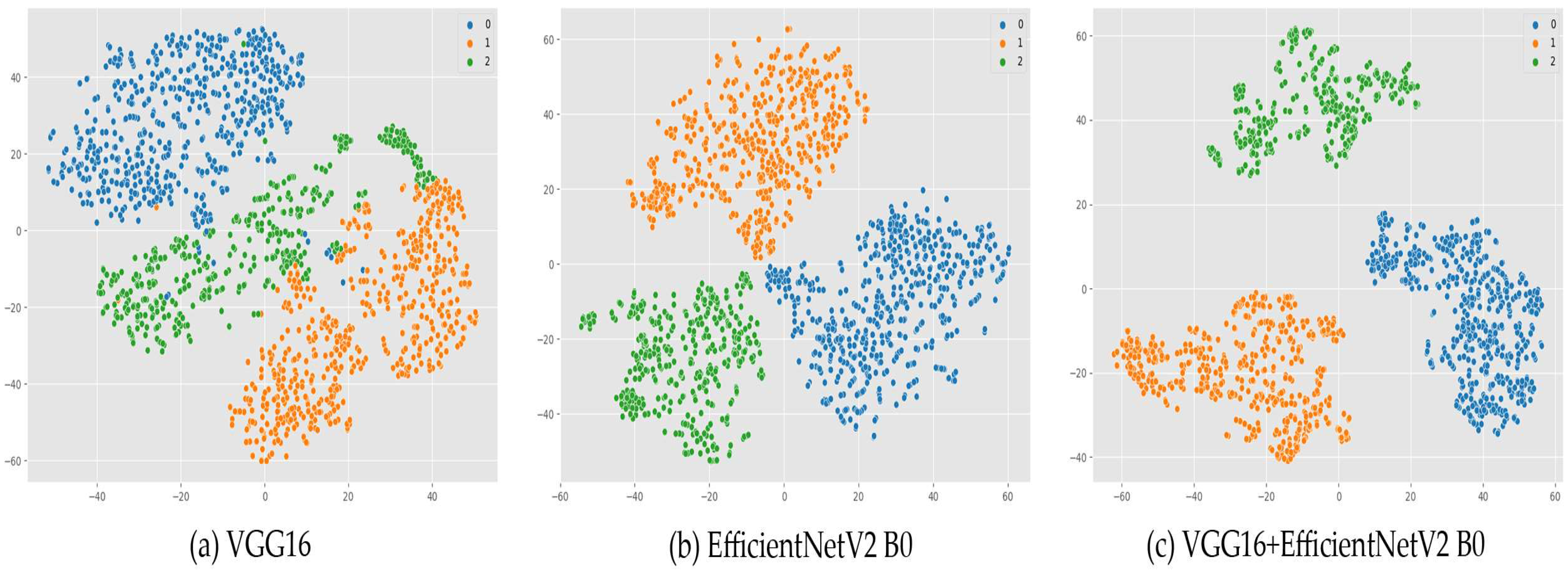
Figure 8a shows the t-SNE visualizations of the feature representations learned by three different models—VGG16, EfficientNetV2B0, and a hybrid model combining VGG16 and EfficientNetV2B0. The three distinct clusters in the t-SNE plot demonstrate VGG16′s effective differentiation between the classes in the dataset.

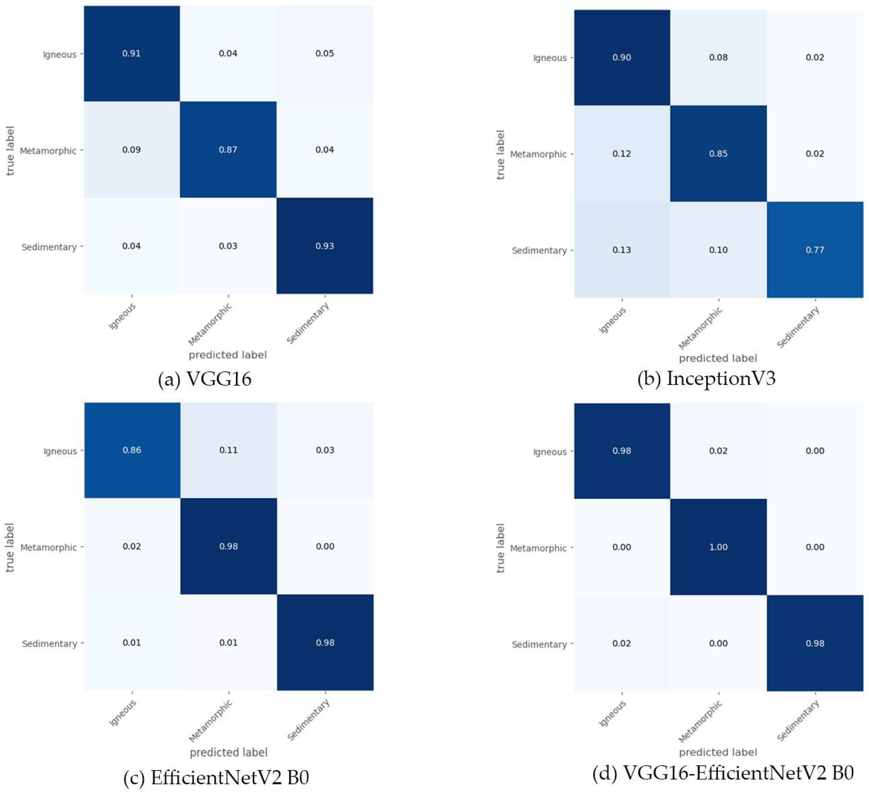
However, some data points are still positioned near the boundaries of clusters, indicating potential misclassifications or overlapping features. In Figure 8b, the t-SNE plot for EfficientNetV2B0 is less distinct compared to VGG16. Particularly, there is overlap between the orange and green clusters, suggesting that EfficientNetV2B0 struggles more than VGG16 in distinguishing certain classes. Figure 8c shows t-SNE visualization of the hybrid model with three well-separated clusters. The combination of VGG16 and EfficientNetV2B0 improves class separation. The clusters are more distinct compared to the individual models, indicating that the hybrid approach leverages the strengths of both models. This also suggests enhanced feature extraction and classification performance and highlights the proposed method’s advantages over other popular deep learning techniques. Figure 9 presents confusion matrices obtained for each model, illustrating performance of different models used in rock-type classification. Each matrix displays the relationships between true and predicted labels along with normalized accuracy rates. According to the results, the VGG16 model produces erroneous results for the metamorphic class, while the Inceptionv3 model shows more errors for the sedimentary class.

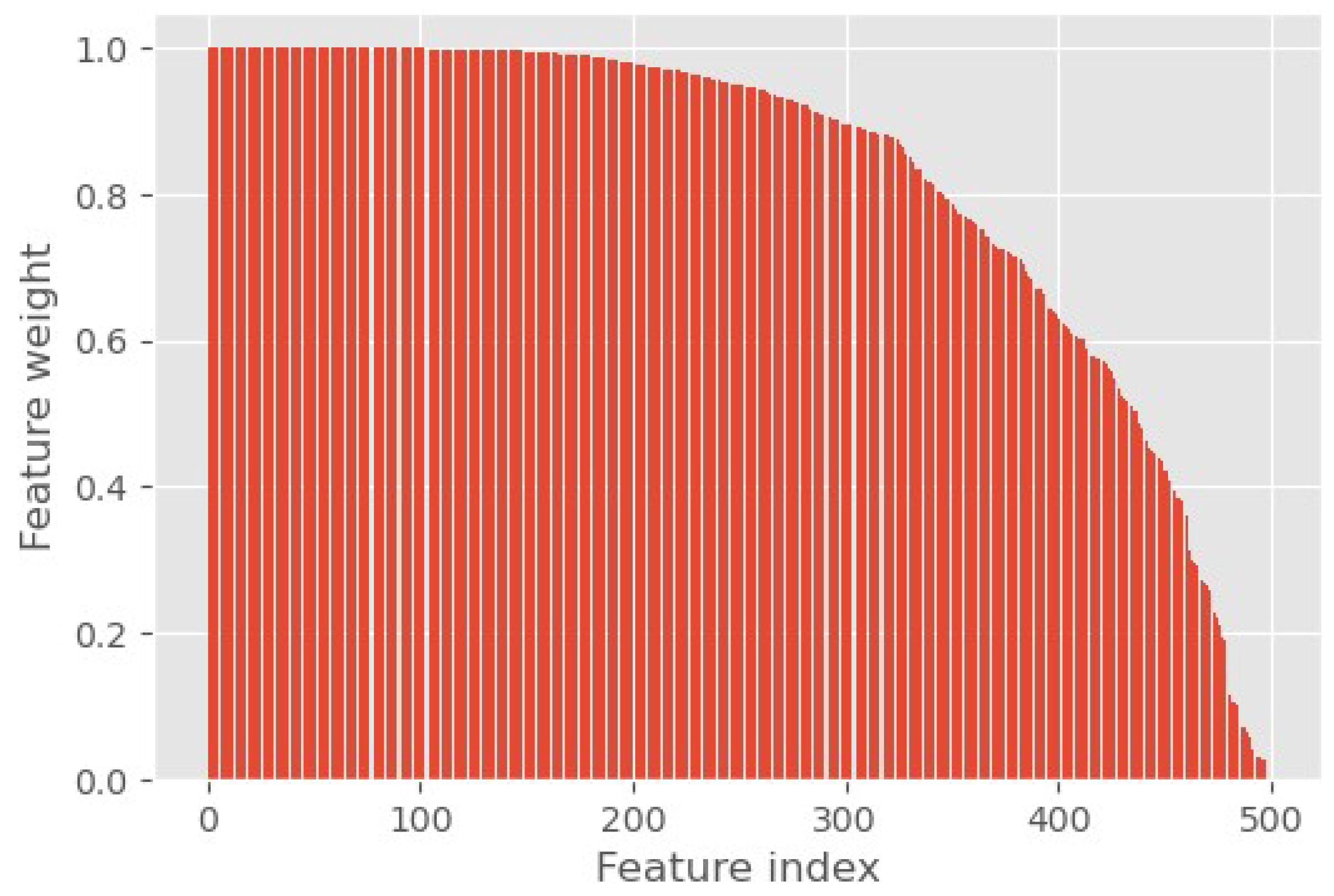
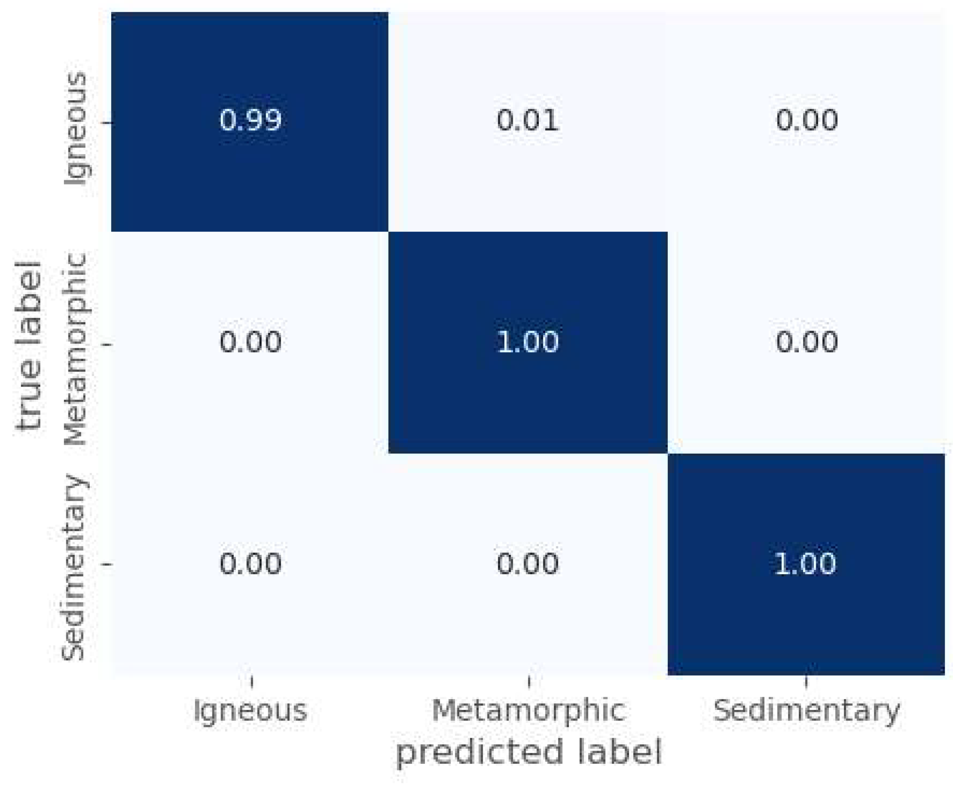
The EfficientNetV2B0 model performs better in both rock groups. Features obtained from the combined EfficientNetV2B0+VGG16 model were subjected to feature selection using the ReliefF algorithm, resulting in the selection of the top 500 features, which were then used as input to the SVM classifier (Figure 10). The classification process was evaluated using five-fold cross-validation. Figure 10 shows that the ReliefF algorithm successfully ranked the most effective features for classification. The top 100 features stand out with high importance scores, while the last 100 features contribute very little to the classification model. High-weighted features significantly enhance model performance, whereas removing low-weighted features allows the model to operate faster and more efficiently. After feature selection with ReliefF, the selected features were used to train the SVM with five-fold cross-validation. Additionally, the C parameter of the support vector machine was determined to be 0.1 through grid search, achieving the best performance. The confusion matrix obtained from cross-validation (Figure 11) highlights the need to extract accuracy, precision, recall, and F1-score values from the confusion matrices to evaluate the performance of the proposed models.

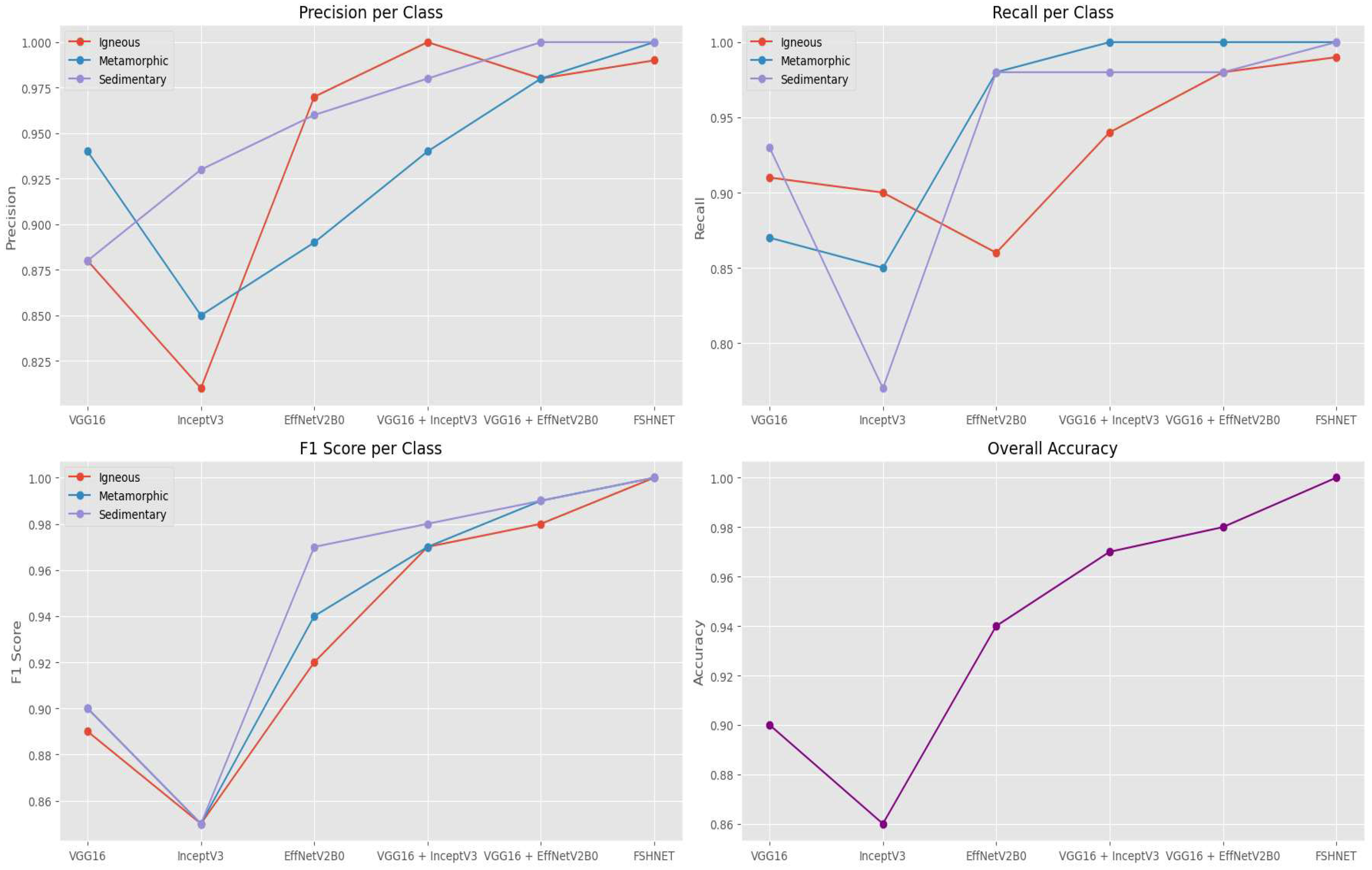
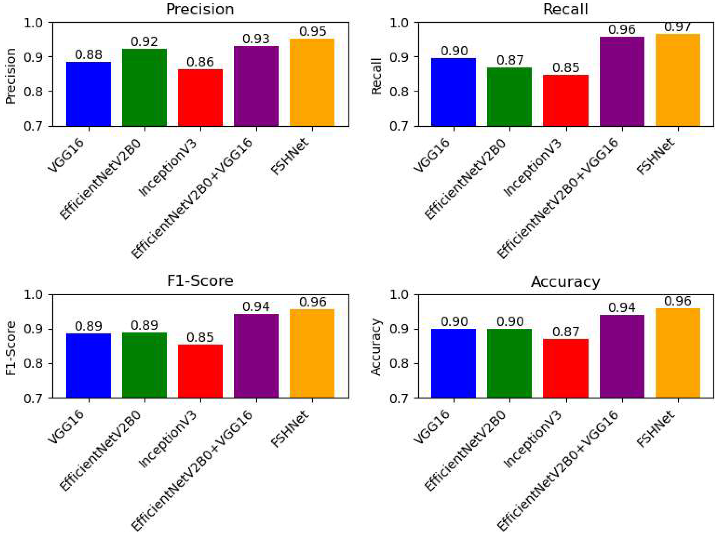
The VGG16+EfficientNetV2B0 hybrid model and FSHNet consistently outperform the other models across all metrics, as shown in Figure 12. These models achieve the highest precision, recall, F1-score, and overall accuracy, demonstrating their superior ability to distinguish between different rock types. The VGG16+EfficientNetV2B0 hybrid model effectively combines VGG16’s rich feature extraction capacity with EfficientNetV2B0’s parameter efficiency and faster training speed. This combination exhibits strong classification performance, particularly for metamorphic and sedimentary rocks, where mineral grain size is smaller compared to magmatic rocks. FSHNet further enhances this performance by optimizing selected features and implementing advanced architectural modifications, resulting in higher accuracy.

The results indicate that hybrid models and advanced architectures such as FSHNet provide significant improvements compared to traditional models like VGG16 and InceptionV3, making them suitable for complex classification tasks such as rock-type identification. Therefore, the use of hybrid and advanced models is recommended for multi-class classification problems requiring high precision and accuracy. To demonstrate the effectiveness of the models, training and testing times were also evaluated (

Table 3. The total training time and test time of each sample for the models used.

Model	Total Training Time (Second)	Test Time per Image (Millisecond)
VGG16	326.73	6.54
InceptionV3	200.86	15.09
EfficientNetV2B0	202.34	13.64
VGG16+InceptionV3	1294.96	9.90
VGG16+EfficientNetV2B0	1065.74	7.21
FSHNet	-	3.32

). The training times of the combined models are longer due to training being performed in two parallel structures. However, inference times of the combined model on the test data remain between those of the two transfer learning models. Especially for the VGG16 and EfficientNetV2B0 models, test time per sample is short. The test time of FSHNet is shorter than the other approaches due to its use of less data. Additionally, when compared with methods used in the literature for classifying thin-section rock images (

Table 4. Comparison of the proposed method with the literature.

Reference	Method	Dataset	Classes	Accuracy (%)
[2]	DenseNet121	Magmatic thin-section rocks	6	98.44
[4]	Resnet50	Pethrographic thin-section rocks	6	96.00
[6]	MSAResnet	Rock thin-section images	3	90.89
[7]	Resnet based XAI	Sedimentary rock thin-section images	6	94.00
[8]	ShuffleNetV2	Rock thin-section images	3	96.00
[9]	Resnet50	Rock thin-section images	3	94.40
[11]	VGG19	Igneous rock type thin-section images	6	97.10
[33]	Concatenated CNN	Pethrographic thin-section rocks	13	89.97
This study	VGG16+EfficientNetV2B0	Rock thin-section images	3	98.00
This study	FSHNET	Rock thin-section images	3	99.66

), the performance of the approaches used to classify different rock types improves when focusing on specific rock types. In the literature, the study by [2] classified six types of magmatic rocks using a DenseNet121-based transfer learning approach, while another study by de Lima et al. [4] employed VGG19, MobileNetV2, InceptionV3, and ResNet50 models to classify different rock types. In both studies, the ResNet50 model achieved the best performance.

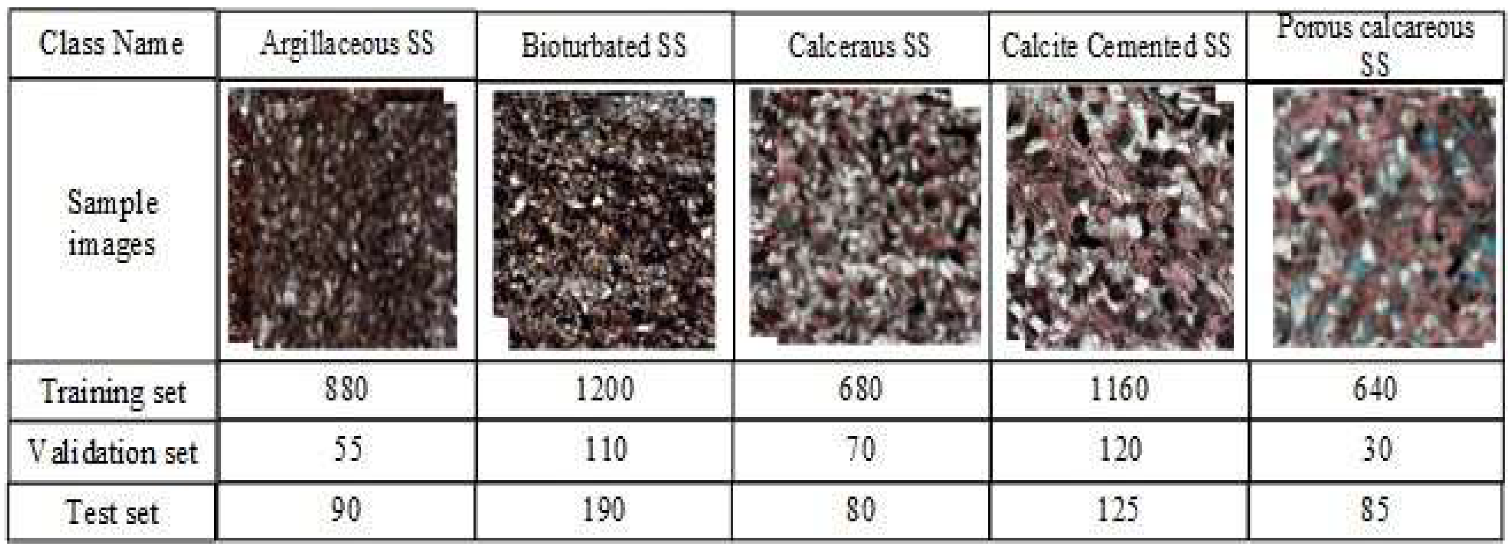
Zheng et al. [7] achieved a 94% accuracy rate in their study to determine sedimentary rock types using ResNet-based explainable artificial intelligence. The rock types were easily distinguishable, and the classification process was conducted by generating heatmaps with explainable artificial intelligence for different scenarios. Seo et al. [11] attained a 97.1% success rate with the proposed VGG19 transfer learning approach to classify igneous rock types, which are included as subrock types in this study. Deep neural networks based on MSA ResNet [6], ShuffleNetV2 [8], and ResNet50 [9] have been proposed for the dataset utilized in this study. While other datasets predominantly focus on one rock type, the dataset employed in this study is divided into three rock types: igneous, sedimentary, and metamorphic. To validate the accuracy and generalization of the proposed method for thin-section images, it was applied to microfacies analysis in rock thin-section images. For this purpose, a dataset consisting of five classes was used: argillaceous siltstone (SS) (0), bioturbated SS (1), calcareous SS (2), porous calcareous SS (3), and massive calcite-cemented SS (4). The numbers in parentheses represent corresponding class labels. Figure 13 presents training, validation, and test samples for each class.

Thin-section rock images captured under 10X magnification using a polarized microscope (Figure 13) were selected for comparing four different classification approaches.

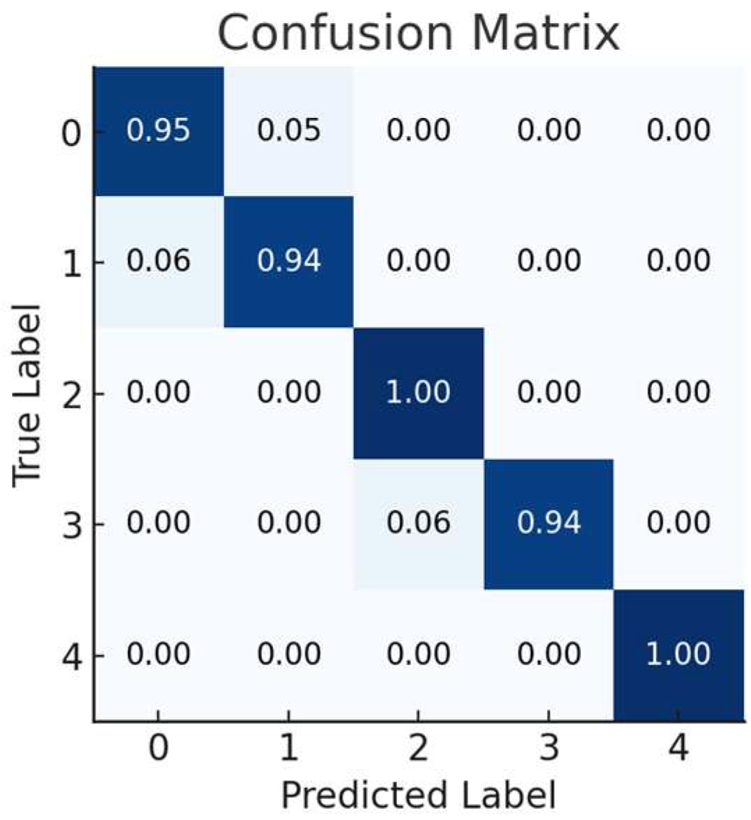
The confusion matrix of FSHNet model (Figure 14) shows a higher accuracy rate compared to other models. The cross-classification errors observed in the other models have been significantly reduced in this approach. Figure 15 illustrates that the FSHNet model outperforms all other models across all evaluation metrics. Additionally, the combined model, which forms the basis of the FSHNet model, achieved the second-highest performance. The models were evaluated not only using validation data from training phase but also with an independent test dataset that was not used during training. This approach measures the generalization ability of models by testing on an independent dataset, indicating whether the model overfits and how well it performs on previously unseen real-world data. The accuracy performance of fine-tuned models for classifying dataset images is compared in

Table 5. Accuracies of different fine-tuned models for thin-section images of petrographic microfacies.

Fine Tuned Model	Training (%)	Validation (%)	Test (%)
VGG19 [4]	100	93	93
MobileNetV2 [4]	100	90	91
Resnet50 [4]	100	89	91
VGG16+EfficientNetV2B0	100	94	93
FSHNet	100	96	95

. The proposed architecture demonstrates strong generalizability across multiple datasets, indicating that its applicability is not restricted to a niche or dataset-specific context (Table 5).

Notably, the combination of VGG16 and EfficientNetV2B0 outperforms the individually utilized models, highlighting the advantage of integrating multiple architectures. The FSHNet model exhibits strong generalization capability by achieving high accuracy on the validation (96%) and test (95%) datasets, which were not used during training. The minimal performance drop compared to the training accuracy (100%) indicates that the model does not suffer from overfitting and can successfully adapt to previously unseen data. These findings confirm that the model does not merely memorize the training data but effectively learns general patterns and distinctive features, ensuring consistent performance across different datasets.

5. Conclusions

In this study, we proposed a new classification system for thin-section rock images using a dual convolutional neural network model that combines the VGG16 and EfficientNetV2B0 architectures. The results indicate that this hybrid approach effectively enhances feature extraction and improves classification accuracy, particularly for challenging classes like metamorphic and sedimentary rocks. The proposed model not only achieves high training and validation accuracy but also demonstrates strong generalization capabilities, avoiding overfitting even with a complex and diverse dataset. The hybrid model’s ability to leverage the strengths of both VGG16 and Efficient-NetV2B0 results in robust performance across all tested metrics, including accuracy, precision, recall, and F1-score. The integration of the ReliefF algorithm for feature selection further optimizes the model by reducing the feature space, which enhances computational efficiency without sacrificing accuracy. Compared to existing deep learning models applied to the same dataset, our approach shows a significant improvement in validation performance, achieving an accuracy increase of more than 3%. This demonstrates the effectiveness of combining different convolutional neural networks for complex classification tasks where distinguishing between similar classes is crucial.

The hand specimen and microscopic appearances of igneous, metamorphic, and sedimentary rocks exhibit fundamental differences. Sedimentary rocks generally exhibit a simple appearance under the microscope. They may contain quartz, calcite, and clay minerals. Minerals other than quartz and calcite are typically very fine-grained and cannot be distinguished. Fossils may be present in these rocks, although not all sedimentary rocks contain fossils. Quartz, however, is always present and has a rounded grain shape. Metamorphic rocks appear similar to igneous rocks under the microscope; however, due to the effect of pressure, their minerals display alignment or banding, referred to as a metamorphic texture. Mineral grains are usually smaller than those in igneous rocks. In addition, certain minerals (e.g., chlorite, muscovite, kyanite) occur exclusively in metamorphic rocks. In microscopic images, features such as mineral shape, color under PPL/XPL, cleavage, and twinning provide essential clues for identifying both the rock type and the minerals it contains. Understanding these microscopic characteristics highlights the complexity of thin-section rock classification and underscores the need for automated, accurate approaches.

Future work could explore the integration of model interpretability techniques to provide more insights into the decision-making process of the model, which is vital for practical applications in geology. Additionally, expanding the dataset to include more diverse samples from different geological settings could further validate the generalizability of the proposed model. Overall, the proposed hybrid convolutional neural network model offers a promising direction for automating the classification of thin-section rock images, contributing to more efficient and accurate geological analysis.

References

1. Li, N.; Hao, H.; Gu, Q.; Wang, D.; Hu, X. A transfer learning method for automatic identification of sandstone microscopy images. Comput. Geosci. 2017, 103, 111–121. [Google Scholar] [CrossRef]
2. Li, H.; He, S.; Radwan, A.E.; Xie, J.; Qin, Q. Quantitative analysis of pore complexity in lacustrine organic-rich shale and comparison to marine shale: Insights from experimental tests and fractal theory. Energy Fuels 2024, 38, 16171–16188. [Google Scholar] [CrossRef]
3. Yu, J.; Wellmann, F.; Virgo, S.; Von Domarus, M.; Jiang, M.; Schmatz, J.; Leibe, B. Superpixel segmentations for thin sections: Evaluation of methods to enable the generation of machine learning training datasets. Comput. Geosci. 2023, 170, 105232. [Google Scholar] [CrossRef]
4. de Lima, R.P.; Duarte, D.; Nicholson, C.; Slatt, R.; Marfurt, K.J. Petrographic microfacies classification with deep convolutional neural networks. Comput. Geosci. 2020, 142, 104481. [Google Scholar] [CrossRef]
5. Aydın, İ.; Kılıç, A.D.; Şener, T.K. Improving Rock Type Identification Through Advanced Deep Learning-Based Segmentation Models: A Comparative Study. Appl. Sci. 2025, 15, 1630. [Google Scholar] [CrossRef]
6. Ma, H.; Han, G.; Peng, L.; Zhu, L.; Shu, J. Rock thin sections identification based on improved squeeze-and-Excitation Networks model. Comput. Geosci. 2021, 152, 104780. [Google Scholar] [CrossRef]
7. Zheng, D.; Zhong, H.; Camps-Valls, G.; Cao, Z.; Ma, X.; Mills, B.; Ma, C. Explainable deep learning for automatic rock classification. Comput. Geosci. 2024, 184, 105511. [Google Scholar] [CrossRef]
8. Li, D.; Zhao, J.; Ma, J. Experimental studies on rock thin-section image classification by deep learning-based approaches. Mathematics 2022, 10, 2317. [Google Scholar] [CrossRef]
9. Wang, B.; Han, G.; Ma, H.; Zhu, L.; Liang, X.; Lu, X. Rock thin sections identification under harsh conditions across regions based on online transfer method. Comput. Geosci. 2022, 26, 1425–1438. [Google Scholar] [CrossRef]
10. Tatar, A.; Haghighi, M.; Zeinijahromi, A. Experiments on image data augmentation techniques for geological rock type classification with convolutional neural networks. J. Rock Mech. Geotech. Eng. 2024, 17, 106–125. [Google Scholar] [CrossRef]
11. Seo, W.; Kim, Y.; Sim, H.; Song, Y.; Yun, T.S. Classification of igneous rocks from petrographic thin section images using convolutional neural network. Earth Sci. Inform. 2022, 15, 1297–1307. [Google Scholar] [CrossRef]
12. Ishikawa, S.T.; Gulick, V.C. An automated mineral classifier using Raman spectra. Comput. Geosci. 2013, 54, 259–268. [Google Scholar] [CrossRef]
13. Das, R.; Mondal, A.; Chakraborty, T.; Ghosh, K. Deep neural networks for automatic grain-matrix segmentation in plane and cross-polarized sandstone photomicrographs. Appl. Intell. 2022, 52, 2332–2345. [Google Scholar] [CrossRef]
14. Yesiloglu-Gultekin, N.; Keceli, A.S.; Sezer, E.A.; Can, A.B.; Gokceoglu, C.; Bayhan, H. A computer program (TSecSoft) to determine mineral percentages using photographs obtained from thin sections. Comput. Geosci. 2012, 46, 310–316. [Google Scholar] [CrossRef]
15. Baykan, N.; Yilmaz, N. Mineral identification using color spaces and artificial neural networks. Comput. Geosci. 2010, 36, 91–97. [Google Scholar] [CrossRef]
16. Singh, N.; Singh, T.N.; Tiwary, A. Textural identification of basaltic rock mass using image processing and neural network. Comput. Geosci. 2010, 14, 301–310. [Google Scholar] [CrossRef]
17. Shang, C.; Barnes, D. Support vector machine-based classification of rock texture images aided by efficient feature selection. In Proceedings of the 2012 International Joint Conference on Neural Networks (IJCNN 2012), Brisbane, Australia, 10–15 June 2012; pp. 1–8. [Google Scholar]
18. Alexandre, P. Editorial for Special Issue “Novel Methods and Applications for Mineral Exploration”. Minerals 2020, 10, 246. [Google Scholar] [CrossRef]
19. Cheng, G.-J.; Ma, W.; Wei, X.-S.; Rong, C.-L.; Nan, J.-X. Research of Rock Texture Identification based on Image Processing and Neural Networks. J. Xi’an Shiyou Univ. 2013, 27, 105–109. [Google Scholar]
20. Lan, X.; Zou, C.; Kang, Z.; Wu, X. Log Facies Identification in Carbonate Reservoirs Using Multiclass Semi-Supervised Learning Strategy. Fuel 2021, 302, 121–145. [Google Scholar] [CrossRef]
21. Pathare, A.R.; Joshi, A.S. Dimensionality Reduction of Multivariate Images Using the Linear & Nonlinear Approach. In Proceedings of the 2023 International Conference on Device Intelligence, Computing and Communication Technologies, (DICCT), Dehradun, India, 17–18 March 2023; pp. 234–237. [Google Scholar]
22. Tariq, A.; Jiango, Y.; Li, Q.; Gao, J.; Lu, L.; Soufan, W.; Almutairi, K.F.; Habib-ur-Rahman, M. Modelling, Mapping and Monitoring of Forest Cover Changes, Using Support Vector Machine, Kernel Logistic Regression and Naive Bayes Tree Models With Optical Remote Sensing Data. Heliyon 2023, 9, e13212. [Google Scholar] [CrossRef]
23. Dabek, P.; Chudy, K.; Nowak, I.; Zimroz, R. Superpixel-Based Grain Segmentation in Sandstone Thin-Section. Minerals 2023, 13, 219. [Google Scholar] [CrossRef]
24. Li, P. Lithological Discrimination Using Aster Image and Geostatistical Texture. J. Mineral. Petrol. 2004, 24, 116–120. [Google Scholar]
25. Fu, P.; Wang, J. Lithology identification based on improved Faster R-CNN. Minerals 2024, 14, 954. [Google Scholar] [CrossRef]
26. Koeshidayatullah, A.; Morsilli, M.; Lehrmann, D.J.; Al-Ramadan, K.; Payne, J.L. Fully Automated Carbonate Petrography Using Deep Convolutional Neural Networks. Mar. Petrol. Geol. 2020, 122, 104–687. [Google Scholar]
27. Wei, W.; Jiang, J.; Qiu, J.; Yu, J.; Hu, X. A photomicrograph dataset of rocks for petrology teaching at Nanjing University. China Sci. Data 2020, 5, 21–33. [Google Scholar] [CrossRef]
28. Zhu, X.X.; Tuia, D.; Mou, L. Deep Learning in Remote Sensing: A Comprehensive Review and List of Resources. IEEE Geosci. Remote Sens. Mag. 2017, 5, 8–36. [Google Scholar] [CrossRef]
29. Simonyan, K.; Zisserman, A. Very deep convolutional networks for large-scale image recognition. arXiv 2014, arXiv:1409.1556 2014. [Google Scholar] [CrossRef]
30. Christianini, N.; Shawe-Taylor, J. An Introduction to Support Vector Machines and Other Kernel-Based Learning Methods 2003; Cambridge University Press: Cambridge, UK, 2003. [Google Scholar]
31. Kononenko, I.; Simec, E.; Robnik-Sikonja, M. Overcoming the myopia of inductive learning algorithms with RELI44 EFF. Appl. Intell. 1997, 7, 39–55. [Google Scholar] [CrossRef]
32. Robnik-Sikonja, M.; Kononenko, I. Theoretical and empirical analysis of ReliefF and RReliefF. Mach. Learn. 2003, 53, 23–69. [Google Scholar] [CrossRef]
33. Su, C.; Xu, S.J.; Zhu, K.Y.; Zhang, X.C. Rock classification in petrographic thin section images based on concatenated convolutional neural networks. Earth Sci. Inform. 2020, 13, 1477–1484. [Google Scholar] [CrossRef]
Figure 1. Example images from dataset. Thin section microscope images of metamorphic rocks (a), igneous rocks (b) and sedimentary rocks (c).
Minerals 15 00976 g001
Figure 2. RGB brightness distributions of dataset.
Minerals 15 00976 g002
Figure 3. EfficientNetv2 B0 model.
Minerals 15 00976 g003
Figure 4. The structure of MBConvolution (a) and Fused-MBConvolution (b) blocks.
Minerals 15 00976 g004
Figure 5. The architecture of VGG16.
Minerals 15 00976 g005
Figure 6. Training and inference pipeline of the architecture.
Minerals 15 00976 g006
Figure 7. Training and loss graphs of each model.
Minerals 15 00976 g007
Figure 8. Trained models feature space he t-SNE representation for base and hybrid models. (a) VGG16, (b) EfficientNetV2B0 and (c) VGG16+EfficientNetV2B0.
Minerals 15 00976 g008
Figure 9. Confusion matrix of proposed method with different models. (a) VGG16, (b) InceptionV3, (c) EfficientNetV2B0 and (d) VGG16-EfficientNetV2B0.
Minerals 15 00976 g009
Figure 10. The feature weights of the top 500 features.
Minerals 15 00976 g010
Figure 11. Confusion matrix for ReliefF-based feature selection and SVM classification.
Minerals 15 00976 g011
Figure 12. Metrics obtained from the confusion matrix for each model.
Minerals 15 00976 g012
Figure 13. Petrographic microfacies dataset with training, validation, and test samples for each class.
Minerals 15 00976 g013
Figure 14. Confusion matrix of the FSHNet model for the petrographic microfacies dataset.
Minerals 15 00976 g014
Figure 15. Performance comparison of five different models on the petrographic microfacies dataset.
Minerals 15 00976 g015