3D Forward Simulation of Borehole-Surface Transient Electromagnetic Based on Unstructured Finite Element Method

Abstract

The time-domain electromagnetic method has been widely applied in mineral exploration, oil, and gas fields in recent years. However, its response characteristics remain unclear, and there is an urgent need to study the response characteristics of the borehole-surface transient electromagnetic(BSTEM) field. This study starts from the time-domain electric field diffusion equation and discretizes the calculation area in space using tetrahedral meshes. The Galerkin method is used to derive the finite element equation of the electric field, and the vector interpolation basis function is used to approximate the electric field in any arbitrary tetrahedral mesh in the free space, thus achieving the three-dimensional forward simulation of the BSTEM field based on the finite element method. Following validation of the numerical simulation method, we further analyze the electromagnetic field response excited by vertical line sources.. Through comparison, it is concluded that measuring the radial electric field is the most intuitive and effective layout method for BSTEM, with a focus on the propagation characteristics of the electromagnetic field in both low-resistance and high-resistance anomalies at different positions. Numerical simulations reveal that BSTEM demonstrates superior resolution capability for low-resistivity anomalies, while showing limited detectability for high-resistivity anomalies Numerical simulation results of BSTEM with realistic orebody models, the correctness of this rule is further verified. This has important implications for our understanding of the propagation laws of BSTEM as well as for subsequent data processing and interpretation.

1. Introduction

With the continuous advancement of national economies and scientific-technological capabilities, global demand for petroleum and mineral resources exhibits sustained growth, driving a heightened emphasis on deep-resource exploration. The urgent need for oil and natural gas resources has prompted a search for electromagnetic exploration methods with higher resolution and stronger anti-noise interference. The well-to-surface transient electromagnetic method—a time-domain electromagnetic technique employing downhole excitation and surface reception—is an electromagnetic exploration method used to detect the electrical structure of underground media. Compared with conventional surface electromagnetic methods, it provides a clearer picture of the response of the deep underground half-space [1]. During the excitation process, the excitation mode where the source is close to the target anomaly will make the response of the anomaly body more obvious., while intrinsic advantages including operational convenience and reduced susceptibility to environmental/climatic constraints, significantly facilitating exploration efficacy.

Previous studies involving borehole-based transient electromagnetic methods have been widely reported. Russia has high-precision field-building induced polarization equipment and comprehensive processing and interpretation technology for both ground and borehole-surface methods [2]. Since the 1990s, an increasing number of experts and scholars in China have begun to engage in research on the borehole-surface electromagnetic method and have gradually put it into practice and application. Xu et al. (1992) [3] first derived the electromagnetic field of a vertical electric dipole source in a layered conductive medium and successfully plotted the distribution characteristics. Later, they (1994) [4] proposed the coefficient recursive relationship of the dipole field in a multi-layer medium. Mao et al. (2010) [5] calculated the electromagnetic field of a vertical electric dipole in a three-layer medium under static conditions and found that the electromagnetic field generated by the dipole in a low-speed state is consistent with that in a static state. He et al. (2011) [6] derived the theoretical solution of the electromagnetic field excited by a vertical wire source, which can be used for theoretical calculation in ground electromagnetic and marine electromagnetic methods. Cao et al. (2012) [7] calculated the electromagnetic field response of a vertical line source in a layered medium. Through the continuous in-depth study of one-dimensional borehole-surface electromagnetic response characteristics, a solid theoretical foundation has been established for its three-dimensional forward numerical simulation.

At the same time, domestic research on the three-dimensional forward modeling of borehole-surface electromagnetic methods has also gradually advanced. Wang et al. (2006) [8] used the finite difference method to conduct three-dimensional numerical simulation research on the borehole-surface direct current method and summarized the basic abnormal patterns. Subsequently, the researchers formulated a three-dimensional forward modeling computational scheme for electromagnetic field responses generated by vertical current sources within stratified media. To detect underground dynamic conductors, Dai et al. (2008) [9] used the finite element method of abnormal potential to achieve a three-dimensional numerical simulation of borehole-surface potential. Ke et al. (2009) [10] completed the three-dimensional forward calculation of the electric field of a vertical finite-length line current source by simplifying the three-dimensional underground medium model using the finite element method, providing foundational theoretical guidance for enhancing inversion quality in the well-to-surface electrical method. Cao et al. (2012) [7] applied the calculation of the borehole-surface electromagnetic field response under horizontal layered medium conditions to the subsequent determination of the oil and gas area range. Zhang et al. (2018) [11] conducted an in-depth analysis of the key factors affecting the electromagnetic field response of a vertical long wire source in a one-dimensional model and found that when the source and the anomalous body are collinear or the measurement point is placed in the well, the borehole-surface electromagnetic method shows higher sensitivity in detecting the anomalous body. Wu et al. (2022) [12] evaluated the rationality and approximation degree of the current loop field, approximating the pure anomalous field based on the borehole-surface joint, providing inspiration for the study of the anomalous field characteristics based on the current loop and the derivation of corresponding interpretation methods. Wang et al. (2022) [13] proposed a three-dimensional forward algorithm for the direct current resistivity method using a hybrid grid finite element method, which has theoretical guiding significance for the forward simulation of both borehole-surface and ground-well resistivity methods. Wu et al. (2022) [12] applied the joint detection of the borehole-surface transient electromagnetic method to deep mineral exploration at a depth of 2000 m, effectively improving the exploration effect in practice. Zhang et al. (2024) [14] investigated the radial electric field response characteristics during the fracturing monitoring of shale gas reservoirs and evaluated the effectiveness of the borehole-surface transient electromagnetic method in the dynamic monitoring of shale gas reservoirs. However, at present, most of the research on borehole-to-surface electromagnetic methods focuses on the frequency domain, while studies on the time-domain borehole-to-surface electromagnetic method are relatively scarce.

Building upon preliminary research of the borehole-to-surface electromagnetic method, this study starts from the time-domain electric field diffusion equation and discretizes the calculation area in space using tetrahedral meshes. The Galerkin method is used to derive the finite element equation of the electric field, and the vector interpolation basis function is used to approximate the electric field in any arbitrary tetrahedral mesh in the free space. A stabilized second-order backward Euler algorithm discretizes the temporal domain, preventing solution oscillations and numerical artifacts. When solving the finite element equations, the PARDISO solver, which offers good computational efficiency and an accurate calculation effect, is selected [15]. It solves large-scale equation systems through LU decomposition and fast back substitution techniques, thereby obtaining the tangential electric field distribution along all tetrahedral mesh edges. Ultimately, by applying the linear interpolation of basis functions, the electric field response at any point in space can be obtained, thus achieving the three-dimensional forward simulation of the borehole-surface transient electromagnetic field based on the finite element method. Based on the verification of the correctness of this simulation method, the response characteristics of the borehole-surface transient electromagnetic field excited by a vertical line source are further analyzed, with a focus on analyzing the propagation characteristics of the borehole-surface electromagnetic field for low-resistance and high-resistance anomalies at different positions. A realistic orebody model, constructed from borehole data of Voisey’s Bay, Labrador, Canada, verifies the practical applicability of these findings for mineral exploration. This provides critical guidance for data processing and interpretation in the borehole-to-surface transient electromagnetic surveys.

2. Basic Theory

2.1. Time-Domain Diffusion Equation

For electrical sources, the transient electromagnetic field is calculated starting from the time-domain Maxwell’s equations. The differential form of Maxwell’s equations is:

$$\nabla \times E\left(r,t\right)=-{\displaystyle \frac{\partial B(r,t)}{\partial t}}$$

(1)

$$\nabla \times H\left(r,t\right)=J\left(r,t\right)+J_s\left(r,t\right)$$

(2)

$$\nabla ·B\left(r,t\right)=0$$

(3)

$$\nabla ·D\left(r,t\right)=\rho \left(r,t\right)$$

(4)

the position vector is $r$, where $E(r,t)$ is the electric field intensity ($\mathrm{V}/\mathrm{m}$); $B(r,t)$ is the magnetic induction intensity ($\mathrm{W}\mathrm{b}/{\mathrm{m}}^2$ or $T$); $H(r,t)$ is the magnetic field intensity ($\mathrm{A}/\mathrm{m})$; and $J(r,t)$ and $D(r,t)$ represen the conduction current density ($\mathrm{A}/{\mathrm{m}}^2$) and the electric displacement vector ($\mathrm{C}/{\mathrm{m}}^2$), respectively. According to the constitutive relationship of macroscopic media:

$$B=\mu H$$

(5)

$$J=\widehat{\sigma E}$$

(6)

where ${\mu }_r$ is the relative magnetic conductivity; $\mu ={\mu }_0{\mu }_r$ is magnetic conductivity (${\mu }_0=4\pi \times {10}^{-7} \mathrm{H}/\mathrm{m}$); and $\widehat{\sigma }$ denotes the conductivity, which is the reciprocal of resistivity. This indicates the ability of materials to conduct current. The time-domain electric field diffusion equation can be derived by eliminating the magnetic field through the simultaneous Equations (1) and (2), obtaining the following [16]:

$$\nabla \times \left[{\displaystyle \frac{1}{\mu }}\nabla \times E\left(r,t\right)\right]+\widehat{\sigma }{\displaystyle \frac{\partial E\left(r,t\right)}{\partial t}}+{\displaystyle \frac{\partial J_s\left(r,t\right)}{\partial t}}=0$$

(7)

2.2. Unstructured Finite Element Method

After obtaining the time-domain electric field diffusion equation, the residual vector is defined according to the Galerkin method as follows. The wave equation is discretized using the finite element method to transform it into the approximate equation of the finite element time-domain (FETD):

$$R\left(r,t\right)=\nabla \times \left[{\displaystyle \frac{1}{\mu }}\nabla \times E\left(r,t\right)\right]+\widehat{\sigma }{\displaystyle \frac{\partial E\left(r,t\right)}{\partial t}}+{\displaystyle \frac{\partial J_s\left(r,t\right)}{\partial t}}$$

(8)

For numerical simulation of complex geological models, each small part is represented by a finite element and filled, thereby discretizing the entire computational region into countless small finite elements. On this basis, we choose tetrahedral elements as the basic shape of the finite element to better meet the diversity of complex geological structures and better adapt to and handle complex geological models. The weighted residual integral is:

$${\iiint }_{\Omega }W\left(r\right)·R\left(r,t\right)dV=0$$

(9)

The weighted residual method aims to find the optimal solution of the equation by minimizing the inner product between the weighting function $W\left(r\right)$ and the residual $R(r,t)$, where $W\left(r\right)$ and $R(r,t)$ are orthogonal. W(r) is the weighting coefficient. Substituting it in, we obtain:

$${\iiint }_{\Omega }W\left(r\right)·\nabla \times \left[{\displaystyle \frac{1}{\mu }}\nabla \times E\left(r,t\right)\right]dV+{\iiint }_{\Omega }W\left(r\right)·\widehat{\sigma }{\displaystyle \frac{\partial E\left(r,t\right)}{\partial t}}dV+{\iiint }_{\Omega }W\left(r\right)·{\displaystyle \frac{\partial J_s\left(r,t\right)}{\partial t}}dV=0$$

(10)

When performing numerical calculations for non-structured tetrahedral mesh discretization, the Nédélec vector interpolation basis functions are selected to ensure the continuity and divergence-free property of the tangential component of the electric field, thereby further improving the calculation accuracy. To effectively express the linear distribution of the electric field inside the element, the electric field at any position of the tetrahedral element is expressed as [17]:

$$E\left(r,t\right)=\sum _{j=1}^6{E}_j\left(t\right)N_j\left(t\right)$$

(11)

where $N_j\left(r\right)$ is the vector interpolation basis function of edge j, and $E_j\left(r\right)$ is the tangential component of the electric field on the j edge. The electric field is interpolated based on the specific properties of the function according to the spatial position r. To make the surface integrals on both sides of the internal interface cancel each other out, the vector interpolation basis function $N\left(r\right)$ is introduced. To satisfy the Sommerfeld boundary condition, the distance between the outer boundary and the source of emission should be sufficiently large. By applying the Galerkin weighted residual method, this can be written in matrix form:

$$SE\left(t\right)+M{\displaystyle \frac{dE\left(t\right)}{dt}}=-J$$

(12)

where S is the global stiffness matrix, M is the mass matrix, and J is the source term. The specific expressions are as follows:

$$S={\displaystyle \frac{1}{\mu }}{\iiint }_{\Omega }\left(\nabla \times N\left(r\right)\right)·\left(\nabla \times N\left(r\right)\right)dV$$

(13)

$$M={\iiint }_{\Omega }N\left(r\right)·\widehat{\sigma }·N\left(r\right)dV$$

(14)

$$J={\iiint }_{\Omega }N\left(r\right)·{\displaystyle \frac{\partial J_s\left(r,t\right)}{\partial t}}dV$$

(15)

The second-order backward Euler difference is used to discretize time, thereby effectively improving the calculation accuracy:

$${\displaystyle \frac{\partial E^{\left(i\right)}}{\partial t}}={\displaystyle \frac{1}{2∆t_i}}\left[3E^{\left(i\right)}-4E^{\left(i-1\right)}+E^{\left(i-2\right)}\right]$$

(16)

Let the time point be numbered as $i$. Substituting Equation (12) into Equation (16), we obtain:

$$\left(3S+2∆t_{i}M\right)E^{\left(i\right)}=S\left[4E^{\left(i-1\right)}-E^{\left(i-2\right)}\right]-2∆t_i{J}^{\left(t\right)}$$

(17)

In this paper, the three-dimensional numerical simulation of TEM adopts step-off excitation. The initial electric field excited by the lower step consists of the electric field of the long wire source and the stable DC electric field formed by the positive and negative electrodes supplying power to the underground. Finally, a large system of equations is formed:

$$K·E=b$$

(18)

3. Algorithm Verification

This paper aims to study the surface and underground electromagnetic field response characteristics of the borehole-surface transient electromagnetic method. To verify the correctness and accuracy of the algorithm used in this paper, a uniform half-space model is established, as shown in Figure 1. The transmitting source is a grounded vertical electric dipole source in the z direction. One end (A) of the transmitting source is located at the surface wellhead, and the other end (B) is located 500 m underground. The transmitting current is 1 A, the air resistivity is 1 × 10⁸ Ω·m, and the surrounding rock resistivity is 100 Ω·m. Three measuring points are set on the surface, and the coordinates of the three measuring points are (200 m, 2000 m, 0 m), (600 m, 2000 m, 0 m), and (1000 m, 2000 m, 0 m). The model locally refines the grid at the transmitter and receiver points, and the final generated grid includes 966,205 domain elements, 25,258 boundary elements, and 818 edge elements.

The analytical solution calculation formula used for verification in this paper is as follows [18]. In the formula, $h$ represents the depth of the electric dipole source, $z$ represents the depth of the measurement point for calculation, where $r$ is the horizontal distance from the ground point (projection point) directly below the source to the observation point, $R_1$ represents the path of electromagnetic waves directly propagating from the source to the observation point, and $R_2$ represents the path of electromagnetic waves after reflection on the ground (processed by the mirroring method to handle boundary conditions). $T_1$ is a dimensionless time parameter related to the real source point and time, $T_2$ is a dimensionless time parameter related to the mirror image source point and time, and $E_r\left(t\right)$ is the radial electric field component generated by the electric dipole source above the conductive half-space in the time domain.

$$\begin{array}{r}{E}_r\left(t\right)={\displaystyle \frac{Idl}{4\pi \sigma }}\{{\displaystyle \frac{\left(h-z\right)}{R_1^5}}\left[3erf\left({\displaystyle \frac{1}{2\sqrt{T_1}}}\right)\right.-{\displaystyle \frac{exp\left(-1/4T_1\right)}{\sqrt{\pi T_1}}}\left.\left(3+{\displaystyle \frac{1}{2T_1}}\right)\right]\\ +{\displaystyle \frac{\left(h+z\right)}{R_2^5}}\left[3erf\left({\displaystyle \frac{1}{2\sqrt{T_2}}}\right)-{\displaystyle \frac{exp\left(-1/4T_2\right)}{\sqrt{\pi T_2}}}\left(3+{\displaystyle \frac{1}{2T_2}}\right)\right]\}\end{array}$$

(19)

$$T_1={\displaystyle \frac{t}{{\mu }_0\sigma R_1^2}} T_2={\displaystyle \frac{t}{{\mu }_0\sigma R_2^2}}$$

(20)

$$R_1^2={\left(h-z\right)}^2+r^2 R_2^2={\left(h+z\right)}^2+r^2 k^2=i\omega {\mu }_0\sigma$$

(21)

We calculated the response values of the electric field component Ex at three different receiving positions and plotted and verified each receiving point. Figure 2 shows the time response curves and error analysis diagrams for each receiving point, respectively. By comparing the finite element solution with the analytical solution of the model, it can be seen that the finite element solution is in good agreement with the analytical solution. The measurement point at 200 m is affected by the source due to the smaller offset distance, while the relative errors of the measurement points at 600 m and 1000 m are both less than 5%. This proves the correctness and accuracy of the time-domain borehole-surface electromagnetic field simulation program written in this paper.

4. 3D Borehole-Surface Model with Anomalous Body

4.1. Deployment Arrangements of Varied Survey Grids

The time-domain borehole-to-surface electromagnetic method encompasses two primary configurations: (1) the Well-to-Surface Electromagnetic Method, wherein the electromagnetic source is transmitted from within the borehole and received at the surface; (2) the Surface-to-Well Electromagnetic Method, wherein the source is transmitted from the surface and received within the borehole [19]. Transmitters for TD-BSEM consist of downhole electrodes (electric sources) or magnetic dipole sources, with transmitted current waveforms comprising zero-based square waves or pseudo-Gaussian pulses. Receiver arrays may be deployed in diverse layouts, contingent upon the geological surface conditions of the surveyed area. In our numerical simulations, regular vertical measurement grids and radial measurement grids were predominantly employed (Figure 3). Prior to conducting three-dimensional forward numerical modeling, homogeneous half-space models with two distinct surface deployment configurations were established to facilitate intuitive analysis of the results.

Figure 4 reveals that the electric field responses (Ex and Ey) acquired using conventional vertical measurement grids exhibit null zones in central regions (the middle area in the x-direction/y-direction of Figure 4), whereas the radial electric field response Er demonstrates no such limitation. Er enables comprehensive visualization of electric field values at arbitrary positions within the receiver area. Thus, in practical borehole-to-surface electromagnetic surveys, it is recommended that the measurement of the radial electric field component (Er) be prioritized in order to facilitate subsequent data processing and analysis. However, in practical field exploration scenarios characterized by rugged terrain, deployment of radial measurement grids demands more stringent ground conditions. As an alternative, conventional measurement grids may be deployed initially, with subsequent transformations of the electric field responses based on coordinate relationships. This approach enhances operational flexibility during field surveys. To facilitate comprehensive understanding of the processes and governing principles of three-dimensional forward modeling for time-domain borehole-to-surface electromagnetic fields, the numerical simulation results presented in this study encompass all electric field components.

$$Er=\sqrt{{Ex}^2+{Ey}^2}$$

(22)

4.2. Single High-Resistance and Low-Resistance Anomalous Body

4.2.1. Low-Resistivity Anomaly Body Model

Based on the principles of borehole-to-surface transient electromagnetic exploration, this study investigates the electric field response characteristics of a single subsurface anomaly. Following validation of the time-domain borehole-to-surface electromagnetic 3D forward modeling algorithm, a low-resistivity anomaly model was established, as illustrated in Figure 5a, for a vertical long wire source measuring 800 m in length in the z-direction, located underground; the coordinates of the two ends of the transmitting electrode were A (0 m, 0 m, −900 m) and B (0 m, 0 m, −100 m). A measurement network was set up on the ground surface, with a measurement point interval of 50 m and 841 measurement points evenly distributed. The transmitting current was 1 A, and the resistivity of the surrounding rock was 100 Ω·m. A low-resistivity anomaly body with a resistivity of 10 Ω·m was placed underground, with a size of 300 m × 200 m × 100 m and the center of the anomaly body located at (300 m, 0 m, −300 m). Unstructured tetrahedral meshing was employed to effectively accommodate complex geological structures, with element size reduction and local refinement implemented at the vertical long-wire source, surface survey grid, and anomaly regions to enhance computational accuracy. The forward model comprised 1,102,483 tetrahedral elements, with the simulation time domain discretized into 955 steps ranging from 2 × 10⁻⁷ s to 1 s.

Figure 6 depicts contour distributions of surface electric field responses at 0.1 ms, 0.5 ms, 0.5 s, and 1 s. It can be seen from the figures that, in the early stage, the electric field response shape is approximately symmetrical, with a negative response on the left and a positive response on the right. As time goes by, in the lossy medium, the electric field response gradually weakens, and the outward propagation of the eddy current can be clearly observed. Prior to encountering the anomaly, both electric field components (Ex and Ey) display source-centered symmetry, where the radial component Er manifests concentric circular patterns in the early phases. When encountering low-resistance anomalies (0.1 s and 1 s), due to the attractive effect of the low-resistance bodies on the current, the electric field response at the corresponding positions significantly weakens, clearly indicating the presence of low-resistance anomalies. This phenomenon indicates that all electric field components can effectively locate the anomalies, confirming that the borehole-surface transient electromagnetic method possesses a good ability to identify low-resistance anomalies.

4.2.2. High-Resistivity Anomaly Body Model

To investigate the detectability of borehole-to-surface electromagnetic methods for high-resistivity anomalies, a geometrically identical high-resistivity anomaly model was established. The remaining parameters of the model remain unchanged. A high-resistivity anomaly body with a resistivity of 1000 Ω·m was placed underground, with a size of 300 m × 200 m × 100 m and the center of the anomaly body still located at (300 m, 0 m, −300 m). Four time points of 0.1 ms, 0.5 ms, 0.5 s and 1 s were selected for observation. The response characteristics of the surface electric field at different time points are shown in Figure 7. Early-stage field diffusion remains observable, with the radial component Er exhibiting concentric circular patterns. As induced currents propagate downward, interaction with the high-resistivity anomaly at 0.1 s and 1 s reveals no discernible field distortion at the target location—in stark contrast to the low-resistivity case. There are no detectable features in all the electric field components, which indicates that the borehole-surface electromagnetic method is unable to identify high resistivity anomalies.

4.3. High- and Low-Resistivity Combined Anomaly Body Model

To investigate the influence of anomaly configuration on detectability in borehole-to-surface electromagnetic methods, a composite high- and low-resistivity anomaly model was established, as depicted in Figure 8, for three-dimensional forward simulation of borehole-surface transient electromagnetic responses. The position of the anomaly body was altered and the number of anomaly bodies increased. The transmitting source remained unchanged, and the same receiving measurement points were set up. Two anomaly bodies with resistivities of 10 Ω·m and 1000 Ω·m were placed, both with a size of 300 m × 200 m × 100 m, and the centers of the anomaly bodies were located at (300 m, 300 m, −300 m) and (300 m, −300 m, −300 m), at two different positions. During model parameterization, the positions of anomalies were altered while increasing their quantity, with the transmitter source retained at the identical location and length. The identical surface receiver array was deployed. Mesh refinement focused on the transmitter, survey grid, and anomalies, yielding a final discretization comprising 1,338,522 domain elements, 64,858 boundary elements, and 1228 edge elements.

Figure 9 presents four contour maps of the surface electric field responses at different times. Not only can it be seen that the electric field shape is approximately symmetrical with respect to the well and the electric field response gradually decreases, but also the secondary field response of a single anomaly body and two anomaly bodies shows morphological differences. Due to the presence of high- and low-resistivity anomalies at different locations underground, compared with a single anomaly body, the existence of low-resistivity bodies at different positions can still be well reflected, but the response to high-resistivity bodies is not sensitive. Given their good ability to identify low-resistivity bodies but inability to identify high-resistivity bodies, it can be seen that low-resistivity anomaly bodies have an attractive effect on the current. This indicates that the borehole-surface transient electromagnetic field has different identification abilities for high- and low-resistivity bodies at different positions, and this rule is not affected by the number or position of the abnormal bodies.

5. Comprehensive Practical Application

5.1. Synthetic Model with Topography

Building upon numerical simulations of anomalies beneath flat terrain, a model incorporating high- and low-resistivity anomalies within complex undulating topography (Figure 10) was developed to investigate the response characteristics of borehole-to-surface transient electromagnetic methods. The air resistivity was set to 1 × 10⁸ Ω·m, with a background resistivity of 10² Ω·m. Two anomalies (10 Ω·m and 1000 Ω·m) identical in size and burial depth (50 m) to those in the flat-terrain model were embedded. Transmitter parameters (location and length) and receiver configurations were maintained identical to prior models for direct topographic comparison. Figure 10b illustrates the mesh discretization, comprising 1,410,592 domain elements, 63,450 boundary elements, and 1253 edge elements. Through the calculation of three-dimensional forward numerical simulation, the response characteristics and patterns of abnormal bodies in complex terrains can be observed, laying a theoretical foundation for the application of time-domain well-earth electromagnetic method in mineral exploration on undulating terrains.

Figure 11 shows the Er contour maps of the electric field response under complex undulating terrain at times 0.1 ms, 0.001 s, 0,01 s, and 0.02 s, both without and with anomalies. The white rectangles in the figure are the projections of the anomalous bodies on the x-y plane, which facilitates a better view of the locations of the two anomalous bodies during analysis. Because the factors of complex and undulating terrain have a significant impact on anomalous bodies of the same size as mentioned above, in order to more intuitively see whether the well electromagnetics method can effectively identify low-resistance anomalous bodies in undulating terrain, two models of anomalous bodies without and with anomalous bodies under the same complex and undulating terrain were calculated.

The uniform half-space model still presents a “concentric circle” shape in the early stage, and the contour lines of the electric field response at each moment are relatively smooth, indicating that the non-structural vector finite element algorithm proposed in this paper can accurately simulate the electric field response of anomalous bodies under complex undulating terrain. In the later stage, it can be clearly seen that the low-resistance anomaly located at the top of the picture is depicted in greater detail. The electric field response value at the center of the corresponding low-resistance anomaly reaches the lowest, which is due to its attractive effect on the current. In contrast, for the high-resistance anomalous body below, the electric field response rapidly decays over time. Due to the relatively shallow burial depth of the anomalous body, its influence gradually weakens, making it insensitive to the identification of high-resistance anomalous bodies. This indicates that in complex and undulating terrains, the time-domain borehole-to-surface electromagnetic method still follows the same rules when identifying high- and low-resistivity anomalies, providing a new theoretical basis for the practical application of mineral exploration.

5.2. Realistic Mineral Deposit Model

Based on the theoretical numerical simulations of previous studies, in order to further explore the influence of actual complex mineral models on the response characteristics of time-domain electromagnetic exploration, we conducted numerical simulations using a real orebody model established based on the drilling information of Voisey’s Bay in Labrador, Canada [20]. According to the known drilling data, Figure 12 shows the drilling exploration model of the ovoid nickel-copper sulfide mining area, which contains a complex orebody with a size of approximately 400 m × 300 m × 115 m. The terrain of the orebody is flat and composed of 70% massive sulfides, with a cover layer thickness of about 20 m (the geometric shape of the ovoid can be ascertained from a large number of drilling activities) [21]. The HEM survey data of this area were synthesized and the results were compared with the real survey data [22]. As shown in Figure 12, the general shape of the complex orebody can be seen, and the overall three-dimensional terrain model is clearly presented [23,24,25]. The resistivity of the orebody is 0.01 Ω·m, and the background resistivity is 1000 Ω·m. Considering the contrast between the resistivity of the orebody and the background resistivity in the above model, we usually choose a more effective and intuitive method to identify the orebody. Therefore, we set the resistivity values of the orebody and the background to 1 Ω·m and 100 Ω·m. A vertical long wire source in the z direction with a length of approximately 335.5 m was set, with the coordinates of the two ends of the transmitter being A (554,950 m, 6,243,090 m, −200 m) and B (554,950 m, 6,243,090 m, −135.5 m). A total of 150 receivers were set, with measurement points spaced 50 m apart, and each measurement line had 10 measurement points. The eastward coordinate range of the observation area was from 555,350 m to 556,050 m, and the northward coordinate range was from 6,242,865 m to 6,243,315 m, this type of spatial partitioning was divided into 966,047 domain units, 49,670 boundary units, and 2386 edge units.

Figure 13 shows the contour map of the Er difference in the electric field response of the complex ovate block sulfide ore body model at 0.001 s, 0.003 s, 0.01 s, and 0.03 s. To clearly distinguish the electric field response anomalies caused by the undulating terrain factors from those of the underground sulfide ore body, we plotted the difference between the calculation results of the abnormal body and the non-abnormal body. Due to the significant differences between the real and complex mineral model and the previously set simple low-resistance anomaly body, including the undulating terrain of the overburden and the large volume of the ore body, the different response characteristics have provided us with a better understanding. As can be seen from Figure 13, the electric field component Er characterizes the ore body accurately and in detail, whether in the early or late stage. This is because the resistivity of the underground oval-shaped blocky sulfide veins is too small, resulting in slow eddy current diffusion. Throughout the entire calculation period of this paper, the abnormal body information can be well reflected. The location of the ore body has been clearly determined. Due to the attraction of the current, the response value at the center position should be relatively low. However, in the figure, the center value of the anomaly body is shown to be the highest value of the electric field response because of the difference. In conclusion, the time-domain borehole-surface electromagnetic detection method can effectively identify ore bodies, which indicates that the borehole-surface electromagnetic method has promising application prospects in the field of mineral exploration.

6. Conclusions

This paper presents a three-dimensional forward simulation of the borehole-to-surface transient electromagnetic field based on the unstructured finite element method. Based on the verification of the correctness of this simulation method, this study initially conducts a systematic analysis of the advantages and limitations of different surface receiver grid configurations. Through the numerical simulation set out in this paper, it can be concluded that:

(1)

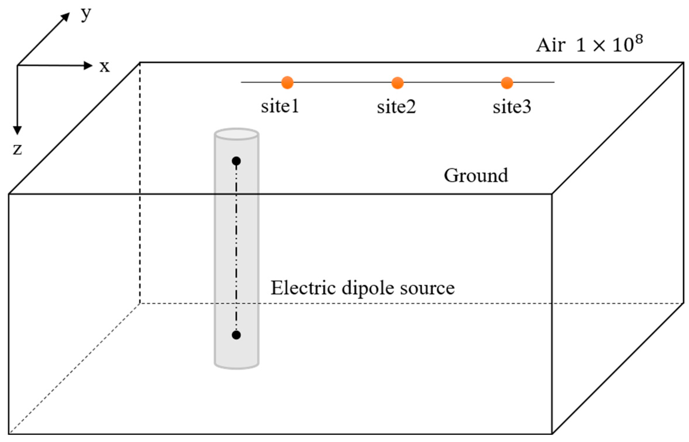
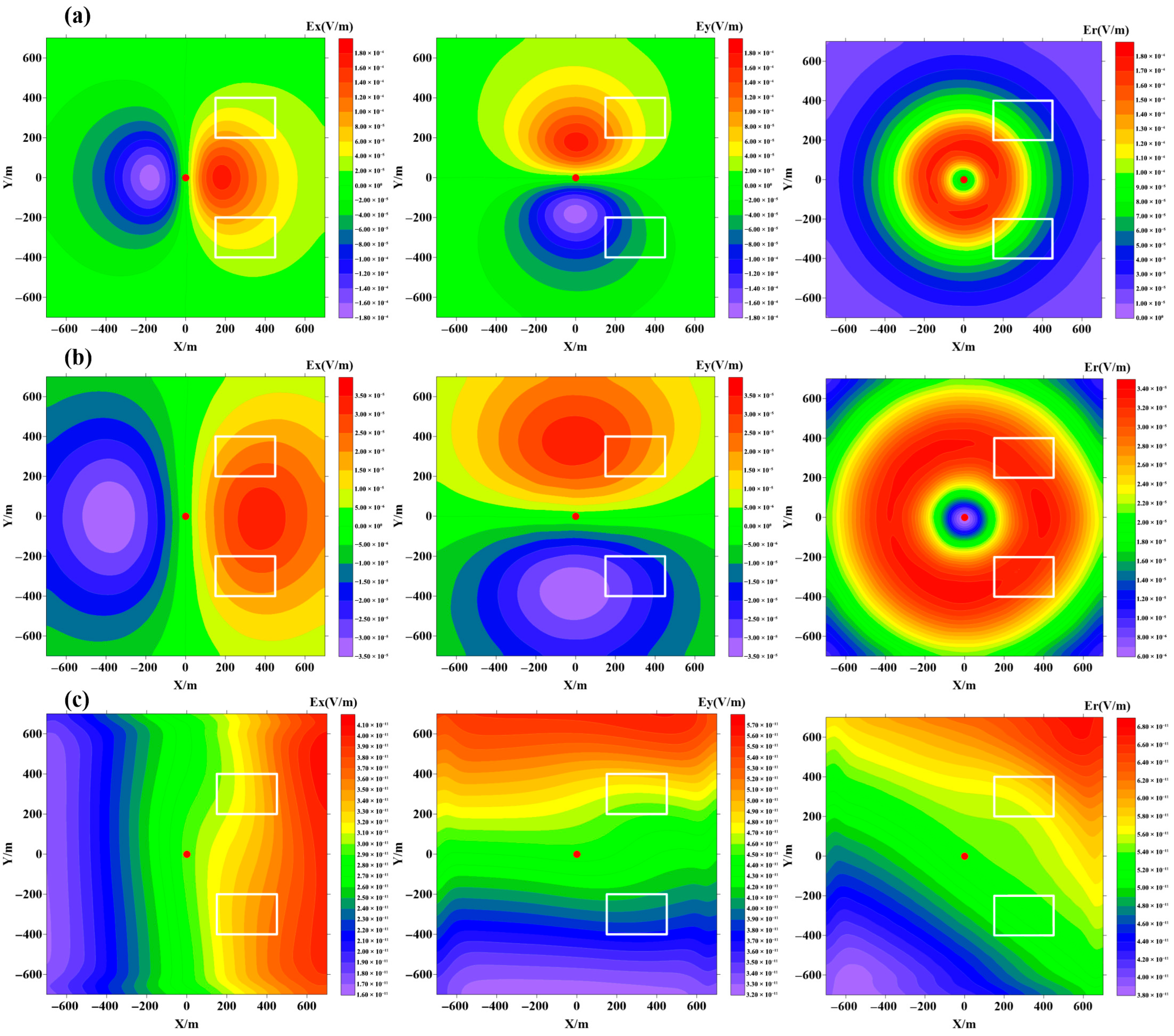
In borehole-to-surface electromagnetic methods, deploying radial measurement grids is optimal for analytical processing of results. When field conditions preclude such deployment, conventional vertical measurement grids may alternatively be deployed, with subsequent computation of the radial electric field.

(2)

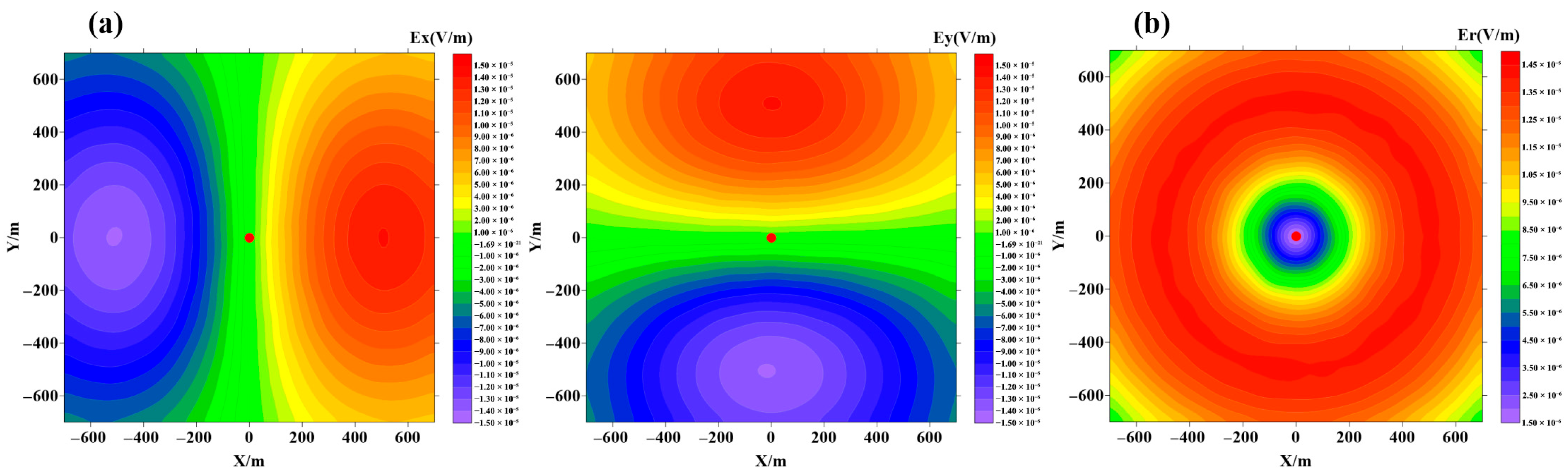
In the early stage, the response shape of the borehole-to-surface transient electromagnetic field is approximately symmetrical with respect to the well, and the signs of the electric field responses on both sides of the well are opposite. With the passage of time, the electric field response gradually weakens.

(3)

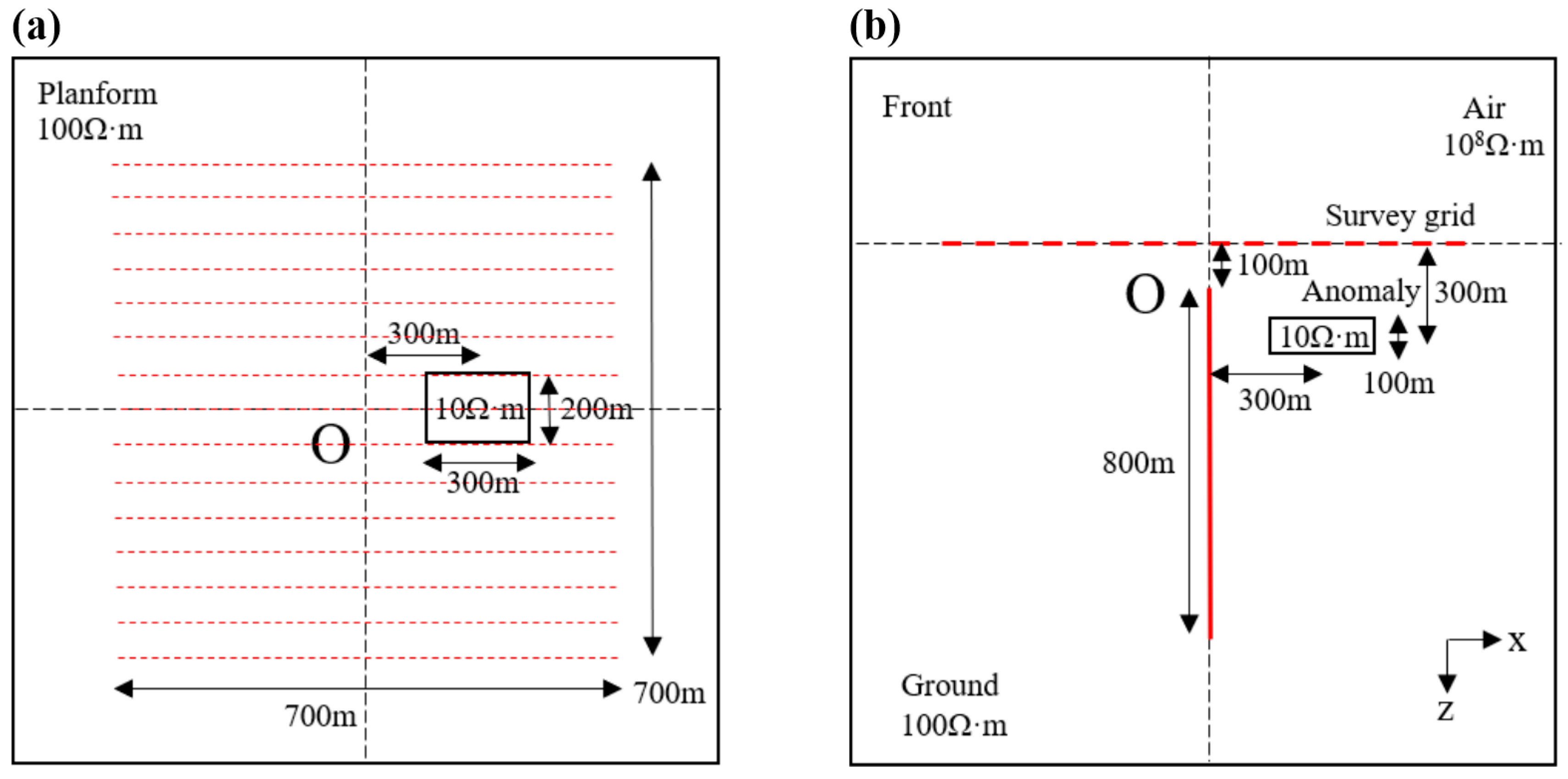
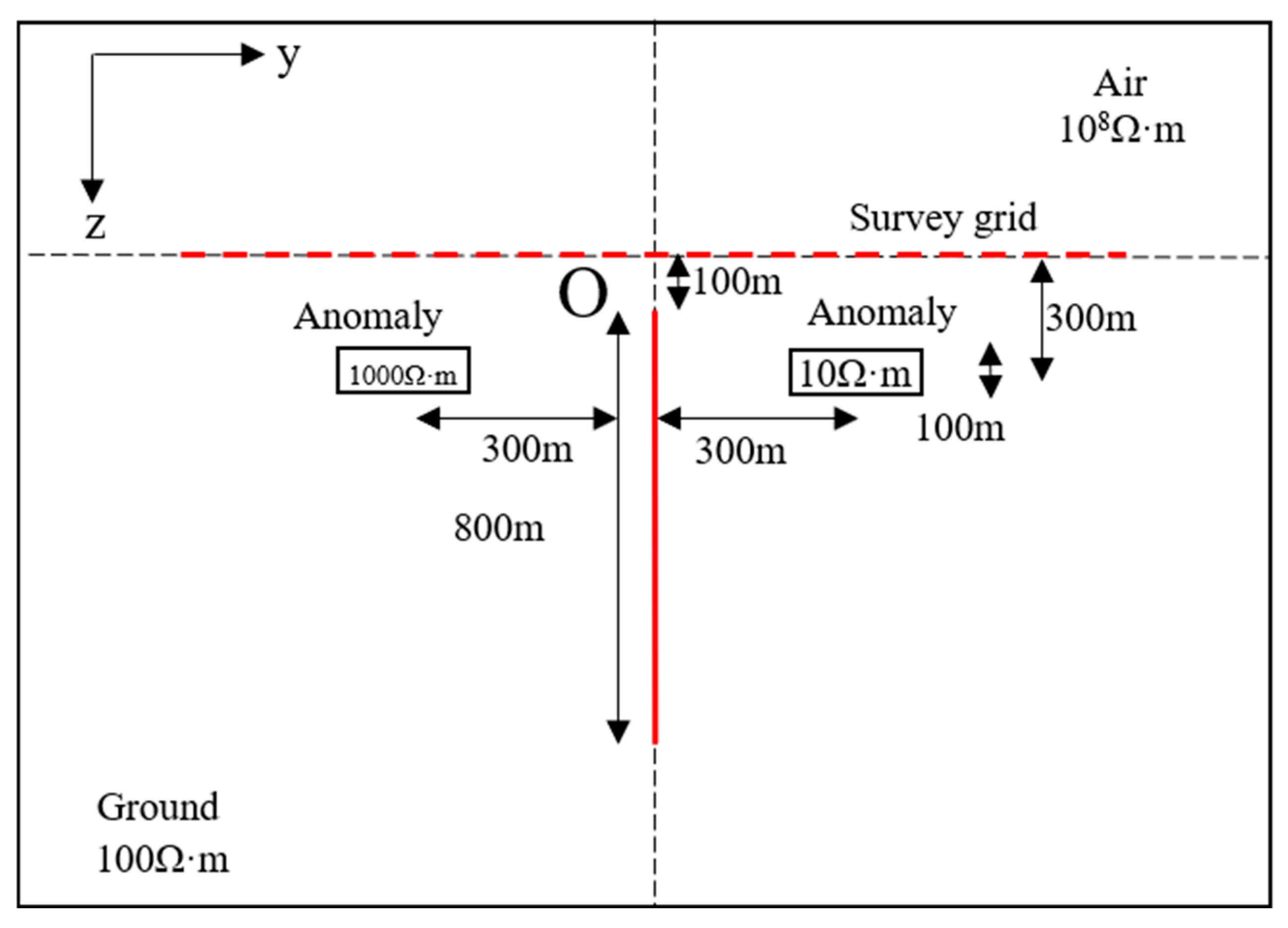
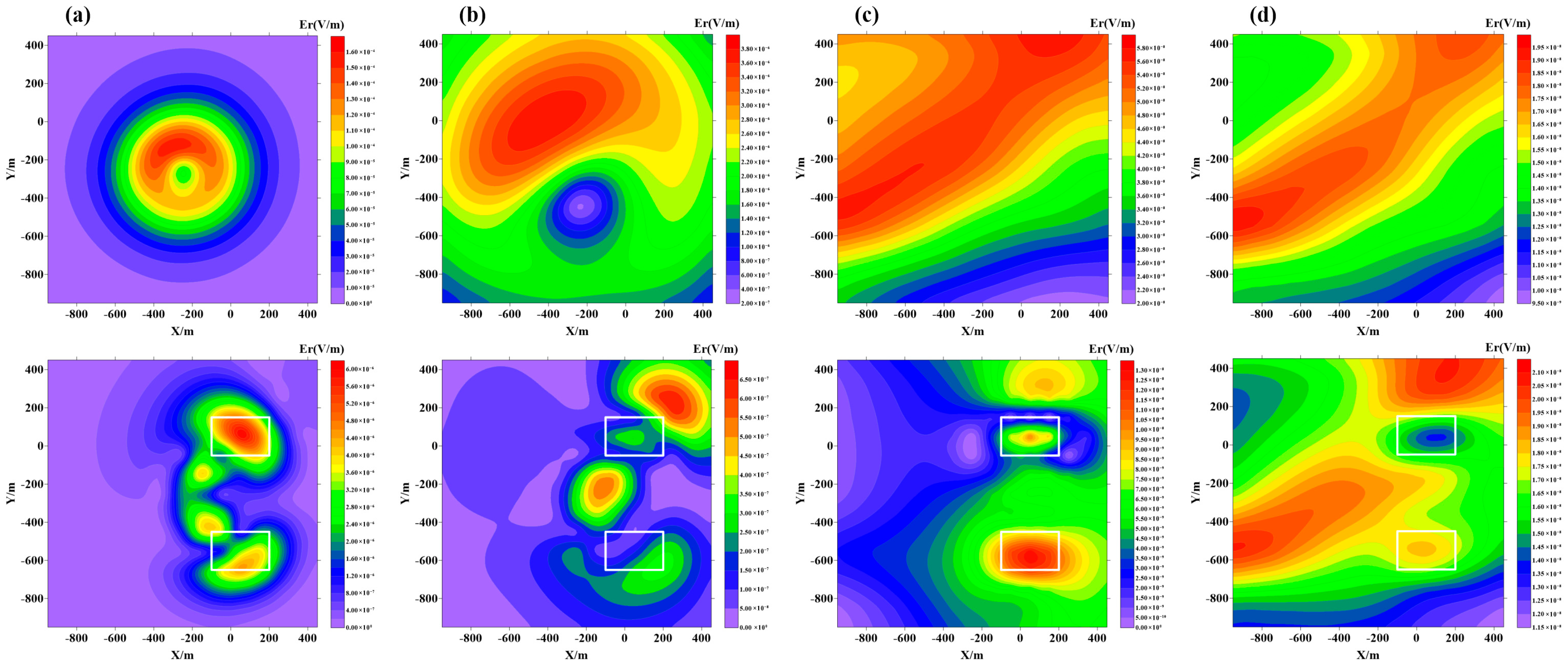
The borehole-to-surface transient electromagnetic field possesses a good ability to identify a single low-resistivity anomaly underground but cannot accurately reflect the existence of a single high-resistivity anomaly. For high- and low-resistivity anomalies at different positions, the same rule is followed. When conducting actual mineral exploration in complex and undulating terrains, the borehole-to-surface electromagnetic method can still effectively identify underground low-resistance ore bodies.

References

1. Li, T.; Wang, J.; Zhu, K. Research on the exploration depth of the borehole-surface electromagnetic field. Prog. Geophys. 2013, 28, 373–379. [Google Scholar] [CrossRef]
2. Zeng, Z.; Zhang, Q.; Wen, B. Progress in geophysical prospecting of Russia. Prog. Explor. Geophys. 2004, 27, 308–311. [Google Scholar]
3. Xu, J.; Hu, W.; Li, P. Electromagnetic fields of a vertical electric dipole in a two-layered conductive media. J. Jianghan. Petroleum. Inst. 1992, 14, 41–44. [Google Scholar]
4. Xu, J.; Zhu, D.; Hu, W.; Li, P. Coefficient recursion relation for dipole fields in multilayer medium. Oil Geophys. Prospect. 1994, 29, 69–74. [Google Scholar]
5. Mao, W.; Zhou, M.; Zhou, Y. EM fields produced by a moving, vertically-directed, time-harmonic dipole in a three-layer medium. J. Harbin Eng. Univ. 2010, 37, 1580–1586. [Google Scholar]
6. He, J.; Bao, L. EM field of vertical wire electric source and its practical meaning. J. Cent. South Univ. 2011, 42, 130–135. [Google Scholar]
7. Cao, H.; Wang, X.; He, Z.; Mao, L.; Lv, D. Calculation of borehole-to-surface electromagnetic responses on horizontal stratified earth medium. Oil Geophys. Prospect. 2012, 47, 338–343. [Google Scholar]
8. Wang, Z.; He, Z.; Liu, Y. Research of Three-Dimensional Modeling and Anomalous Rule on Borehole-Ground DC Method. Chin. J. Eng. Geophys. 2006, 3, 87–92. [Google Scholar]
9. Dai, Q.; Chen, D.; Xiong, J.; Feng, D. The 3-D Finite Element Number Modeling of Vertical Line Source Borehole Ground DC Method Detecting Underground Dynamic Conductor. Chin. J. Eng. Geophys. 2008, 5, 643–647. [Google Scholar]
10. Ke, G.; Huang, Q. 3D Forward and Inversion Problems of Borehole-to-Surface Electrical Method. Acta Sci. Nat. Univ. Pekin. 2009, 45, 264–272. [Google Scholar]
11. Zhang, J. 3D Electromagnetic Forward Modeling of Vertical Finite-length Wire Source. Master’s Thesis, China University of Geosciences, Beijing, China, 2018. [Google Scholar]
12. Wu, J.; Liu, B.; Zhi, Q.; Deng, X.; Wang, X.; Yang, Y.; Lu, D.; Qiu, J. Application of surface and borehole TEM joint exploration in 2 000 m deep mineral exploration. Coal Geol. Explor. 2022, 50, 70–78. [Google Scholar] [CrossRef]
13. Wang, X.; Wang, C.; Mao, Y.; Yan, L.; Zhou, L.; Gao, W. 3D forward modeling of DC resistivity method based on finite element with mixed grid. Coal Geol. Explor. 2022, 50, 136–143. [Google Scholar] [CrossRef]
14. Zhang, W.; Xie, X.; Zhou, L.; Wang, X.; Yan, L. 3-D forward modeling of shale gas fracturing dynamic monitoring using the borehole-to-ground transient electromagnetic method. Front. Earth Sci. 2024, 12, 1394094. [Google Scholar] [CrossRef]
15. Bollhofer, M.; Eftekhari, A.; Scheidegger, S.; Schenk, O. Large–scale sparse inverse covariance matrix estimation. SIAM J. Sci. Comput. 2019, 41, A380–A401. [Google Scholar] [CrossRef]
16. Um, E.S.; Harris, J.M.; Alumbaugh, D.L. 3D time-domain simulation of electromagnetic diffusion phenomena: A finite-element electric-field approach. Geophysics 2010, 75, F115–F126. [Google Scholar] [CrossRef]
17. Jin, J.M. The Finite Element Method in Electromagnetics; John Wiley & Sons: Hoboken, NJ, USA, 2014. [Google Scholar]
18. Barsukov, P.O.; Fainberg, E.B. The field of the vertical electric dipole immersed in the heterogeneous half-space. Izv. Phys. Solid Earth 2014, 50, 568–575. [Google Scholar] [CrossRef]
19. Hu, Z.Z.; He, Z.X.; Li, D.C.; Liu, Y.X.; Sun, W.B.; Wang, C.F.; Wang, Y. Reservoir monitoring feasibility study with time lapse magnetotellurics survey in Sebei Gas Field. Oil Geophys. Prospect. 2014, 49, 997–1005. [Google Scholar] [CrossRef]
20. Jahandari, H.; Farquharson, C.G. Finite-volume modelling of geophysical electromagnetic data on unstructured grids using potentials. Geophys. J. Int. 2015, 202, 1859–1876. [Google Scholar] [CrossRef]
21. Balch, S.; Crebs, T.; King, A.; Verbiski, M. Geophysics of the Voisey’s Bay Ni-Cu-Co deposits. In SEG Technical Program Expanded Abstracts 1998; Society of Exploration Geophysicists: Houston, TX, USA, 1998; pp. 784–787. [Google Scholar]
22. Garrie, D.G. Dighem survey for diamondfields resources Inc. Archeanresources Ltd. Voisey’s Bay, Labrador, Survey Report 1202, Dighem, A division of CGG Canada Ltd. 1995. [Google Scholar]
23. Li, J.; Hu, X.; Cai, H.; Liu, Y. A finite-element time-domain forward-modelling algorithm for transient electromagnetics excited by grounded-wire sources. Geophys. Prospect. 2020, 68, 1379–1398. [Google Scholar] [CrossRef]
24. Jahandari, H.; Farquharson, C.G. A finite-volume solution to the geophysical electromagnetic forward problem using unstructured grids. Geophysics 2014, 79, E287–E302. [Google Scholar] [CrossRef]
25. Li, J.; Lu, X.; Farquharson, C.G.; Hu, X. A finite-element time-domain forward solver for electromagnetic methods with complex-shaped loop sources. Geophysics 2018, 83, E117–E132. [Google Scholar] [CrossRef]
Figure 1. Schematic diagram of the uniform half-space validation model.
Minerals 15 00785 g001
Figure 2. Accuracy verification for the homogeneous half space at different measurement points.
Minerals 15 00785 g002
Figure 3. Layout methods of grounded survey lines for well-surface electromagnetic method.
Minerals 15 00785 g003
Figure 4. The calculation results of the two different measurement grid arrangements at 0.01 s. (a) regular survey grid; (b) radial survey grid.
Minerals 15 00785 g004
Figure 5. Schematic diagram of a single anomaly body model. (a) overhead view of the model; (b) front view of the model.
Minerals 15 00785 g005
Figure 6. Distribution map of the electric field component response for individual low-resistance anomaly models at different time intervals. The white rectangular wireframe represents the projection of the low-resistance anomaly on the horizontal plane in each picture. (a) 0.1 ms; (b) 0.5 ms; (c) 0.5 s; (d) 1 s.
Minerals 15 00785 g006
Figure 7. Distribution map of the electric field component response for individual high-resistance anomaly models at different time intervals. The white rectangular wireframe represents the projection of the high-resistance anomaly on the horizontal plane in each picture. (a) 0.1 ms; (b) 0.5 ms; (c) 0.5 s; (d) 1 s.
Minerals 15 00785 g007aMinerals 15 00785 g007b
Figure 8. Schematic diagram of high- and low-resistivity combined anomaly body model.
Minerals 15 00785 g008
Figure 9. Distribution map of the electric field component response for high- and low-resistivity combined anomaly body models at different time intervals. The white rectangular wireframe at the top of the picture represents the projection of the low-resistance anomaly on the horizontal plane in each picture, while the one at the bottom is used to represent the high-resistance anomaly body. (a) 0.1 ms; (b) 0.5 ms; (c) 0.5 s; (d) 1 s.
Minerals 15 00785 g009aMinerals 15 00785 g009b
Figure 10. Schematic diagram of synthetic model with topography. (a) The positions of the source, receiver and anomalous body in undulating terrain; (b) discretization of anomaly model under undulating terrain. The red line represents a long grounded-wire transmitter, the blue points represent the receivers, the red cuboids represent low-resistance outliers, and the green ones represent high-resistance outliers.
Minerals 15 00785 g010
Figure 11. The distribution map of the electric field component response of the high- and low-resistivity combined anomaly body model under undulating terrain. The white rectangular wireframe at the top of the picture represents the projection of the low-resistance anomaly on the horizontal plane in each picture, while the one at the bottom is used to represent the high-resistance anomaly body. (a) 0.1 ms; (b) 0.001 s; (c) 0.01 s; (d) 0.02 s.
Minerals 15 00785 g011
Figure 12. Schematic diagram of realistic mineral deposit. (a) The locations of the source, receivers and ore body; (b) discretization of the mineral deposit model. The red line represents a long grounded-wire transmitter, and the blue points represent the receivers.
Minerals 15 00785 g012
Figure 13. Distribution map of the electric field component Er response for realistic mineral deposit model at different time intervals. The shape of the white box in the picture represents the projection of the rough outline of the real sulfide ore body on the ground level. (a) 0.001 s; (b) 0.003 s; (c) 0.01 s; (d) 0.03 s.
Minerals 15 00785 g013
Disclaimer/Publisher’s Note: The statements, opinions and data contained in all publications are solely those of the individual author(s) and contributor(s) and not of MDPI and/or the editor(s). MDPI and/or the editor(s) disclaim responsibility for any injury to people or property resulting from any ideas, methods, instructions or products referred to in the content.