Modern Capabilities of Semi-Airborne UAV-TEM Technology on the Example of Studying the Geological Structure of the Uranium Paleovalley

Abstract

Unmanned systems provide significant prospects for improving the efficiency of electromagnetic geophysical exploration in mineral prospecting and geological mapping, as they can significantly increase the productivity of field surveys by accelerating the movement of the measuring system along the site, as well as minimizing problems in cases where the pedestrian walkability of the site is a challenge. Lightweight and cheap UAV systems with a take-off weight in the low tens of kilograms are unable to carry a powerful current source; therefore, semi-airborne systems with a ground transmitter (an ungrounded loop or grounded at the ends of the line) and a measuring system towed on a UAV are becoming more and more widespread. This paper presents the results for a new generation of semi-airborne technology SibGIS UAV-TEMs belonging to the “line-loop” type and capable of realizing the transient/time-domain (TEM) electromagnetics method used for studying a uranium object of the paleovalley type. Objects of this type are characterized by a low resistivity of the ore zone located in relatively high-resistivity host rocks and, from the position of the geoelectric structure, can be considered a good benchmark for assessing the capabilities of different electrical exploration technologies in general. The aeromobile part of the geophysical system created is implemented on the basis of a hexacopter carrying a measuring system with an inductive sensor, an analog of a 50 × 50 m loop, an 18-bit ADC with satellite synchronization, and a transmitter. The ground part consists of a galvanically grounded supply line and a current source with a transmitter creating multipolar pulses of quasi-DC current in the line. The survey is carried out with a terrain drape based on a satellite digital terrain model. The article presents the results obtained from the electromagnetic soundings in comparison with the reference (drilled) profile, convincingly proving the high efficiency of UAV-TEM. This approach to pre-processing UAV–electrospecting data is described with the aim of improving data quality by taking into account the movement and swaying of the measuring system’s sensor. On the basis of the real data obtained, the sensitivity of the created semi-airborne system was modeled by solving a direct problem in the class of 3D models, which allowed us to evaluate the effectiveness of the method in relation to other geological cases.

1. Introduction

Geophysical data collection technologies using lightweight unmanned systems have become a significant feature of the geological prospecting industry [1]. The use of unmanned aerial vehicles (UAVs) as carriers allows geophysical data to be obtained at a much higher speed in comparison with traditional pedestrian methods, and UAV technologies are much more affordable in comparison to traditional aerial methods, which are cost-effective only in areas of hundreds of square kilometers [2]. Geophysical methods such as magnetic prospecting or gamma-ray surveys have mostly been implemented in UAV variants in the recent past, at least in those countries where light UAV flights are possible without serious restrictions [2,3,4,5,6,7]. Electrical prospecting survey systems on UAV carriers appeared much later since the obvious problem is the realization of a current source system on a UAV, but now there are several solutions available—radio wave-type systems without a controlled source [8,9] and two traditional approaches to measurements in the frequency domain (FDEM) and time domain (TEM/TDEM). The more thoroughly developed direction is that involving frequency measurements by magnetometers or a vertical inductive frame [10,11,12,13,14]. Time-domain measurements have been the subject of limited research until recently, but such work has become increasingly common in recent years [15,16,17,18,19].

Known technologies applicable to geological prospecting and geotechnical problems include so-called semi-airborne systems, in which the EM field source, heavy for a lightweight UAV, is located on the ground, and the lightweight sensor is towed on the UAV since only this option allows for a depth in the hundreds of meters region to be achieved. The most recent TEM systems explored in the literature implement a loop-to-loop geometry, which assumes that a large generator loop is stretched around the study area [18]. According to the authors, this approach is of little use for geological prospecting tasks and is better suited for situations such as studying small areas that are dangerous for people, for example, those with landslide hazards. For several years, the authors have been developing technologies with semi-airborne electromagnetic sounding SibGIS UAV-TEM with an unconventional combination of a source and receiver “line-loop”; in such geometry, the formation of an electromagnetic field in a geological environment is carried out using a transmitter line grounded at the ends, which is usually several kilometers long, and from each such line it is possible to perform a survey over an area with a side approximately equal to its length [16]. Measurements were made using the field establishment method, using a vertical inductive frame in the time domain—the magnetic component was measured with $\partial {\mathit{B}}_{\mathit{z}}/\partial t$.

The ambition of the author’s team is to achieve the possibility of completely replacing traditional ground-based sensing with airborne methods. UAV–electrospecting systems have been in development since 2020 and have been undergoing continuous improvements over the years to improve the quality of data and depth of soundings, and this paper considers the capabilities of the current version in solving the problem of building geoelectric sections in a fairly common geological case involving the search for mineralization in a paleovalley. In addition, in order to assess the effectiveness of the technology in a general case, the numerical modeling of non-stationary electromagnetic fields is performed on the basis of real data obtained, and the sensitivity of the current version of the UAV-TEM technology to anomalous objects is evaluated. Vitimskiy-type uranium deposits, which are used as a model object due to the geological study carried out on them [20] and the simplicity of the model from the point of view of geoelectrics, are ideal for evaluating the sensitivity of the transient method and testing new electrical prospecting systems.

2. Materials and Methods

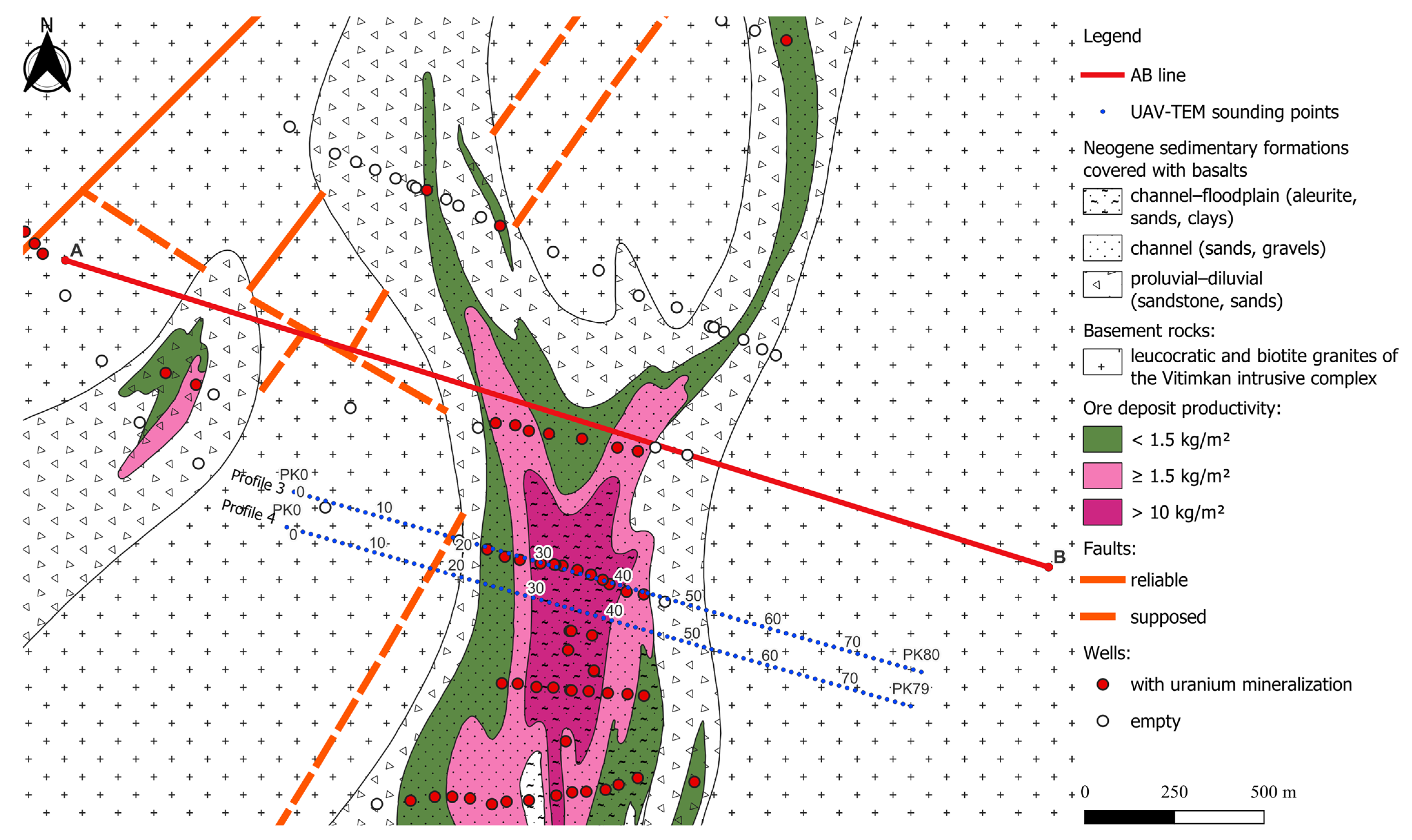
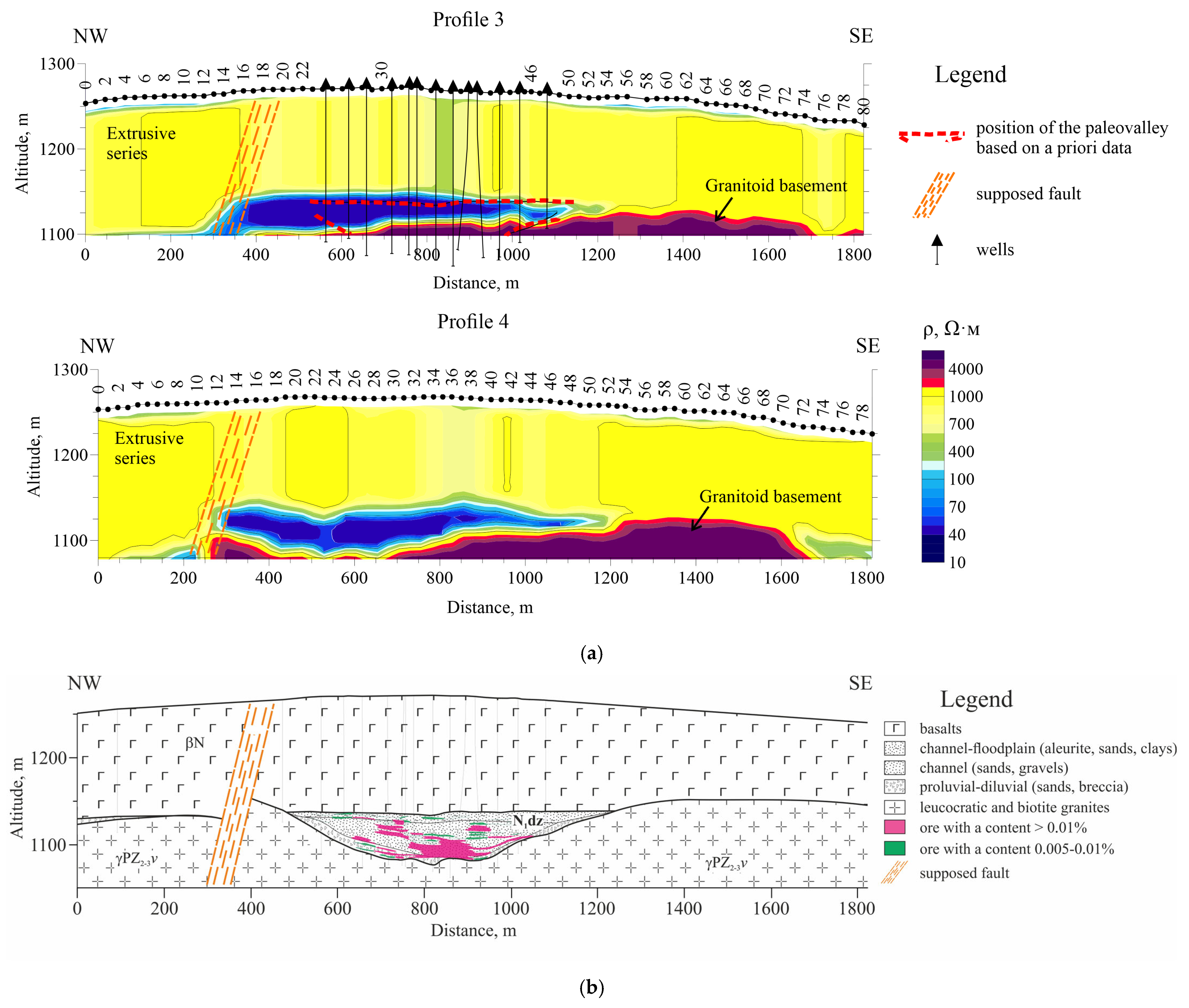
2.1. Geological Model of the Site

The Khiagdinskoye deposit is located in Southern Transbaikalia (East Siberia), 190 km north of the city of Chita. According to [21], the geological structure of the Vitim uranium-ore district is determined by its location on the southeastern periphery of the Baikal arch uplift, the formation of which began in the late Oligocene period. The vault uplift involved deeply eroded Baikal and Caledonian fold structures, which became the basement used for the accumulation of Neogene continental sediments and Neogene–Quaternary plateau basalts.

Vitimsky-type uranium deposits belong to the exogenous genetic class of the infiltration paleolithic type. Uranium mineralization is confined to paleodoline structures cut into the crystalline basement (see Figure 1). It gravitates to the basal parts of the Miocene sediments section, forms linearly oriented deposits with a length of 800–5900 m and width of 20–300 m, and occurs at depths of 60–240 m from the surface. Sometimes, mineralization occurs in the weathering crust along the boundaries of the crystalline basement (Figure 1). In reference [20], the formation of uranium mineralization of this type is described in detail, and an average uranium content of 0.05% is indicated. Ore-bearing rocks are characterized by increased iron sulfide content. The associated minerals include pyrite, marcasite, galena, sphalerite, arsenopyrite, etc. [21].

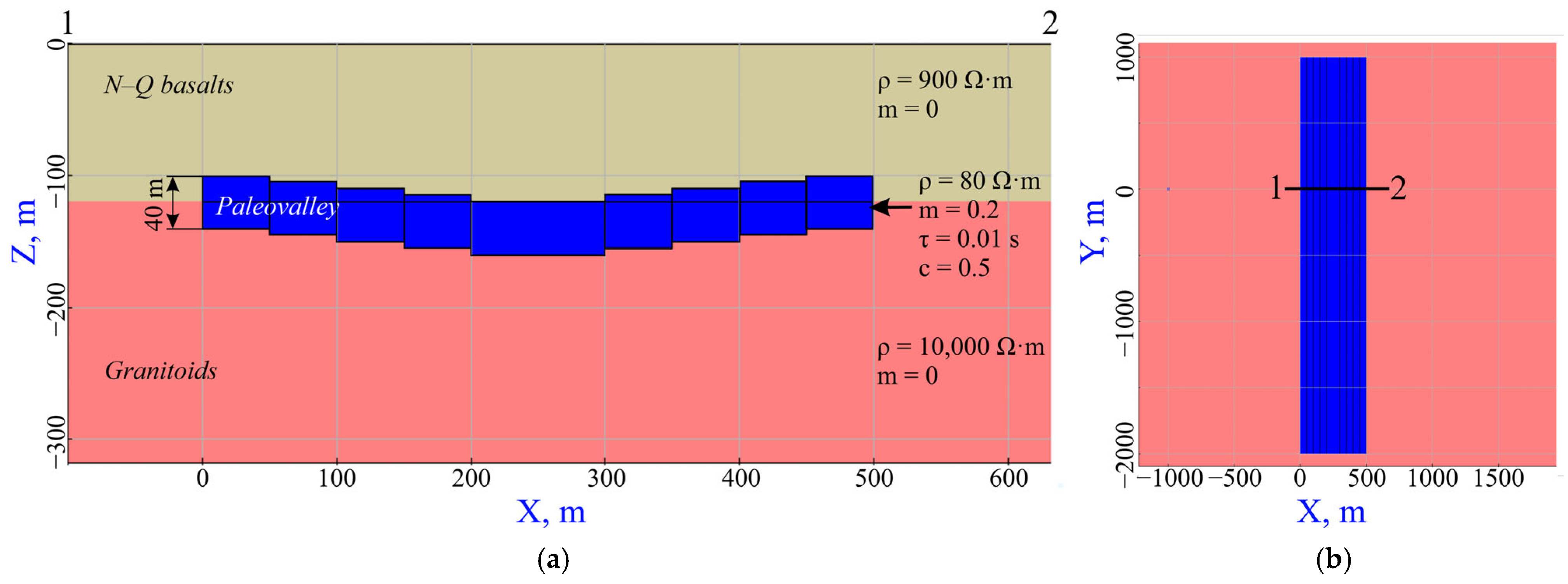
2.2. Physical–Geological Model of the Deposit

Based on the geology of the Vitimsky-type deposits and a priori information, an initial physical–geological model (PGM) was compiled. The physical properties of rocks of the paleovalley model in the first approximation can be approximated as follows:

• The effusive stratum (several covering layers of basalt separated by interlayers of tuffs and interformational sediments, with an average thickness of 130 m) is characterized by medium density (2.5 g/cm³), high magnetic susceptibility (2.0–230 SI units), high resistivity (900–8000 Ω·m), and medium acoustic velocity (3800 m/s);
• Productive sediments (sands, clays, and grus with a thickness of 40–150 m) have a low density (2.0 g/cm³), weak magnetism (0.24 SI units), low resistivity (40 Ω·m), and low velocity (2150 m/s);
• Crystalline basement rocks (granitoids, diorites, limestone, metamorphic schists, and sandstone) have high density (2.45–2.82 g/cm³), low-to-moderate magnetic susceptibility (0.4–0.73 SI units), a wide range of specific resistivity based on resistivity logging (190–2000 Ω·m), and high acoustic velocity (4300 m/s).

This PGM, from the perspective of electrical exploration, is quite simple: it is conventionally a three-layer model. On top is the overlying basalt stratum with high resistivity; below it is the target low-resistivity layer, confined to dealluvial–proluvial sedimentary rocks, where uranium mineralization may be located. The lowest layer is the granite basement.

For the PGM, the target object (in the form of a paleovalley) was approximated by several rectangular parallelepipeds with the following parameters: resistivity (ρ) = 80 Ω·m; chargeability (m) = 0.2; relaxation time (τ) = 0.01 s; and frequency exponent (c) = 0.5. These parameters describe polarizability properties within the widely used Cole—Cole phenomenological model [22] in the adapted version for complex conductivity by Pelton [23]. Each parallelepiped has dimensions of 50 × 3000 × 40 m (XYZ) and is positioned in close contact with the adjacent ones, with a 5 m offset along the Z-axis (except for the central ones), arranged to form a lens-shaped (or trough-like) structure in the cross-section along the X-axis. Since the depth of uranium mineralization, based on the geological description, can reach up to 240 m from the surface, in the PGM, we decided to increase the thickness of the basalt overlap layer to 120 m. The depth to the top of the object is up to 100 m at the edges of the paleodoline and up to 120 m in the center. This complicates the task for the transient method in the unmanned version (UAV-TEM). The resistivity of the Neogene–Quaternary basalts is 900 Ω·m, and that of the basement granitoids is 10,000 Ω·m. The layers are non-polarizable (see Figure 2).

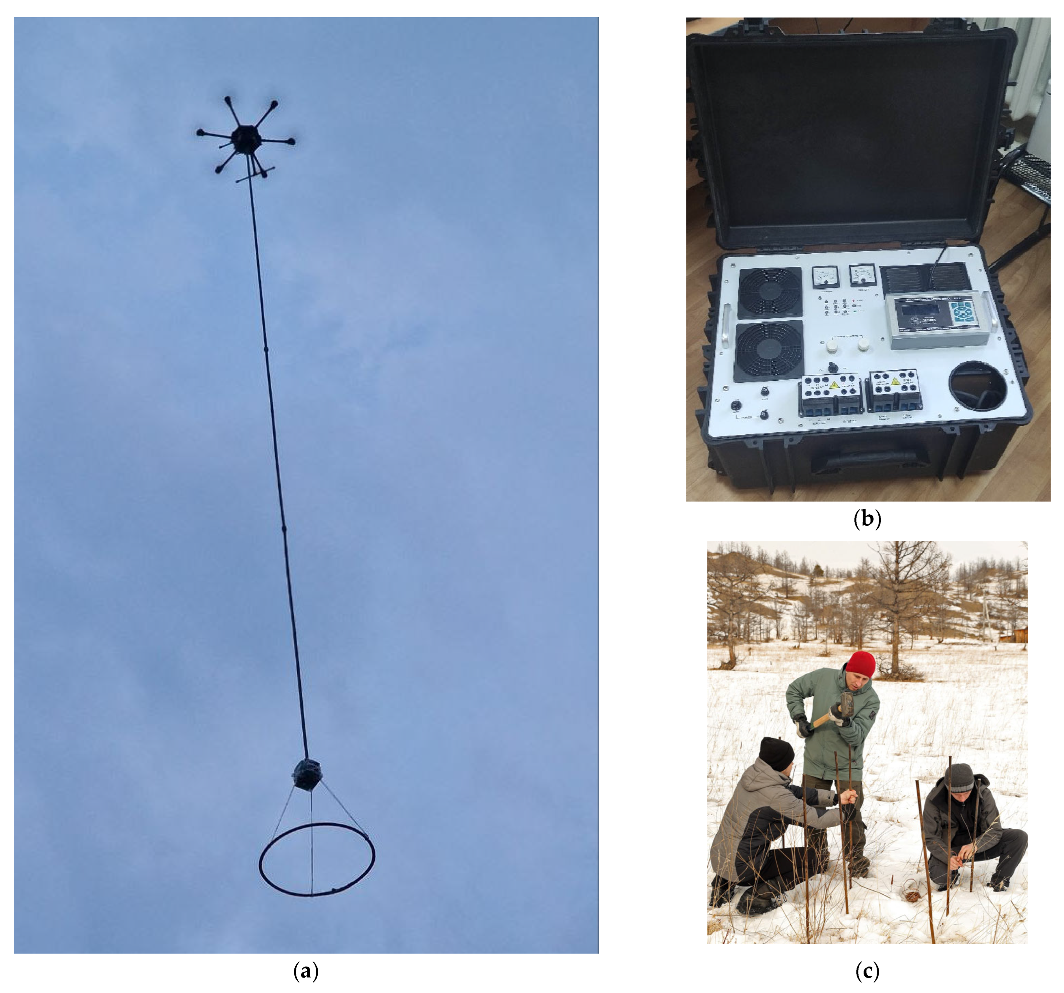
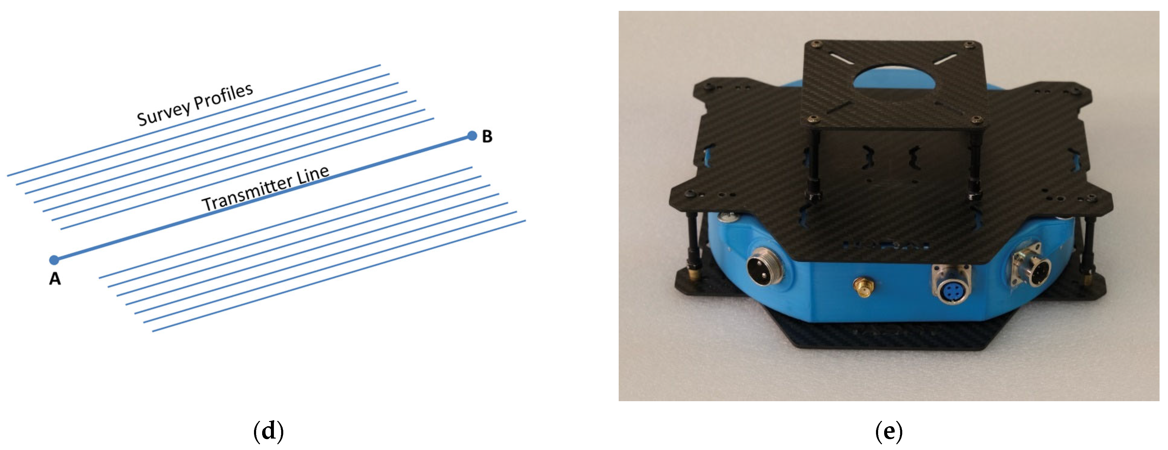
2.3. SibGIS UAV-TEM Technology

Despite the fact that, over the years, the capabilities of the previous versions of the SibGIS UAV-TEM system have been described several times in the literature [9,16,17], this system is constantly being developed; therefore, the characteristics of the variant used in this work are given below.

As noted earlier, the TEM technology is semi-airborne: the transmitter line, AB, galvanically grounded at the ends with 20–30 steel electrodes at 1.5 m long, is located on the ground, and a sequence of multipolar rectangular current pulses of a given duration is fed through it. Transient curves are recorded using a vertical magnetic sensor (inductive frame), i.e., the change in the vertical magnetic field $\partial {\mathit{B}}_{\mathit{z}}/\partial t$ is measured. Registration is carried out using a two-channel recorder, in which each channel is galvanically isolated, and 18-bit serial approximation analog-to-digital converters (ADCs) with a signal sampling frequency of 100 kHz are used. The satellite time with an error of up to 1 μs is used for the synchronization of transmitter and receiving systems.

A compact multiwinding frame [24] with a diameter of 0.9 m and an effective area of 2500 m², adapted for use with UAVs, is employed as a receiving sensor. The initial signal registration time is 20–30 µs. The frame is mounted on a 10 m long hose attached to the UAV. The entire measurement system has a mass of 4 kg. An unmanned system with a six-rotor copter is used as a carrier. The UAV with receiving equipment flies along pre-created routes parallel to the AB line (Figure 3d).

The primary data are averaged at a given step using Hampel’s robust M-estimation [25].

The UAV’s cruising speed is 9–10 m per second to minimize measurement sensor oscillations, and the suspension material also smooths out jerks and oscillations. Depending on the length of the transmitter line and the geoelectric characteristics of the geological section, it is possible to survey an area of up to the low tens of square kilometers from one take-off point. In the current version of the current source and switch (

Table 1. Characteristics of transmitter/current source KER-100 and receiver/measuring system.

KER-100 Current Switch
Amplitude of stabilized current pulses	0.1–100 A;
Maximum output voltage	950 V
Maximum power output	54,000 W
Duration of current pulses in pulse (+)-pause-pulse (−)-pause mode	0.01, 0.1, 0.125, 0.25, 0.5, 1, 2, 4, 8 s
Pulse repetition error	1 µs
Current amplitude setting error	Not more than 1%
Satellite systems	GPS/GLONASS
Protection complies with IP 54
Possibility of synchronization with the measuring system by GNSS time
MARS v2.0 ADC and measuring unit
Number of channels	2
Compensation for voltage offset of electrode potentials	±1 V
Input impedance not less than	20 MΩ
Gains	0.25, 0.5, 1, 2, 4, …, 128
Sampling frequency	100 kHz
ADC digit capacity	18 bits
Maximum input signal	±4.096 V.
Battery power	12 V (range: 10 V to 15 V).
Current consumption (approx.)	max. 0.3 A
Satellite time synchronization	GPS/GLONASS/Galileo/BeiDou

), it has become possible to generate up to 50 pulses per second, and even taking into account the need for data smoothing to improve the quality of the curves, the semi-airborne system provides very high data density, in comparison with both ground surveys, where the density of sounding points was economically limited, and in comparison with airborne systems, where with similar or lower data acquisition frequency, the flight speed was multiple times higher.

Thus, an important advantage of the semi-aerial UAV–electromagnetic survey is not only the ability to speed up and reduce the cost of geophysical measurements in conditions with difficult pedestrian accessibility areas but also the acquisition of very detailed data (on 10 × 50 m level grids) on fairly large individual sites.

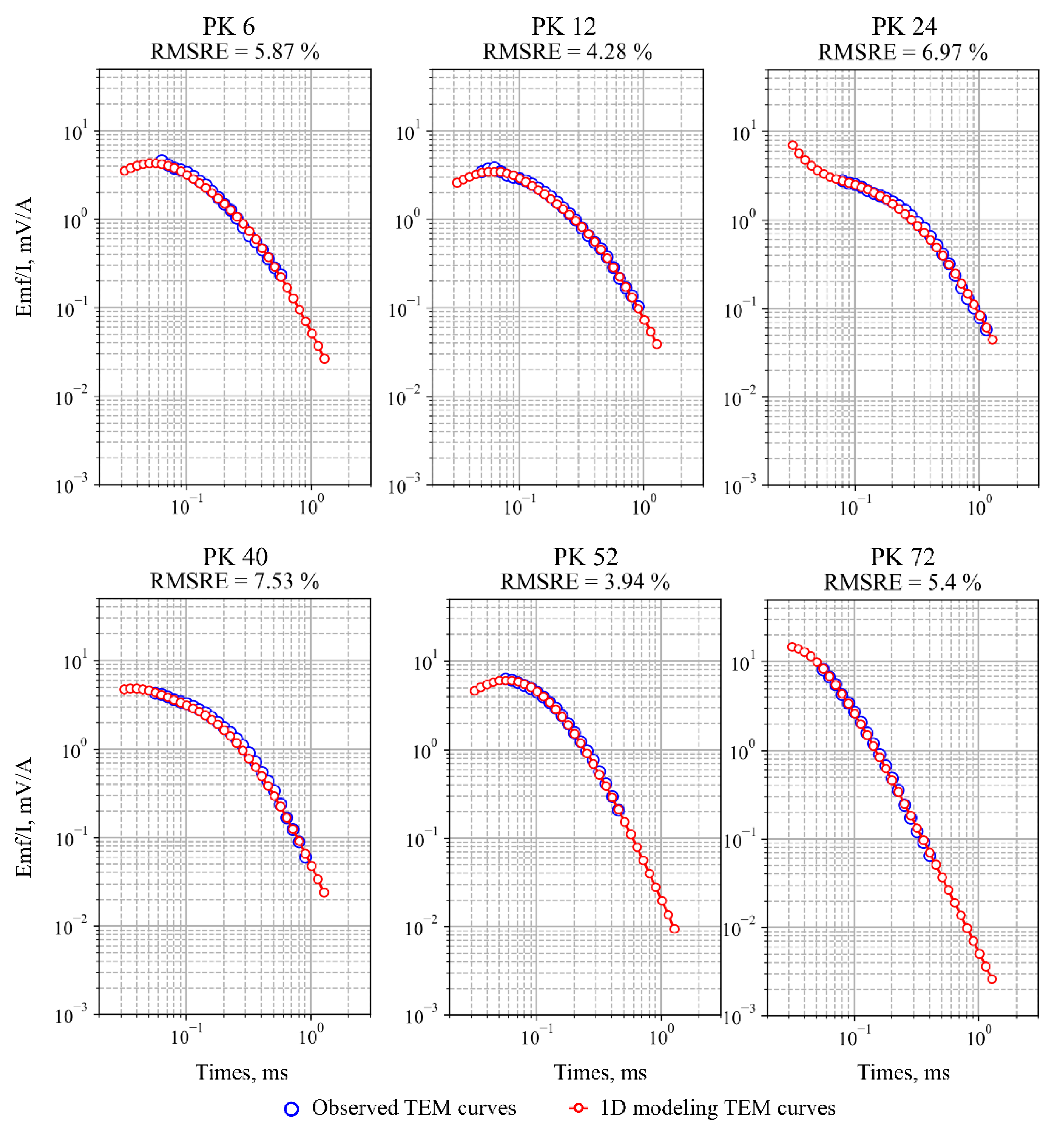
2.4. Solution to the 1D-Inverse Problem

The solution to the inverse problem within the framework of one-dimensional models was carried out in the Mars1D one-dimensional inversion program. The calculations of the direct problem were performed in the frequency domain, but the formation curves were set in time. For the AB-q setup used, which records only $\partial {\mathit{B}}_{\mathit{z}}/\partial t$, the expression for calculating the vertical magnetic component of the EM field in the frequency domain is as follows (1)–(12) [26]:

$$H_z=-{\displaystyle \frac{p}{4{\pi }^2}}{\displaystyle \frac{\partial }{\partial y}}\underset{-\mathrm{\infty }}{\overset{\mathrm{\infty }}{\iint }}{\displaystyle \frac{R^H}{n_1+n_0{R}^H}}{e}^{-i\left(k_{x}x+k_{y}y\right)}d{k}_{x}d{k}_y,$$

(1)

$$n_j=\sqrt{k_x^2+k_y^2-k_j^2},$$

(2)

$$k_j=\sqrt{i\omega {\mu }_0{\sigma }_j},$$

(3)

$$R^H=\coth \left(n_1{d}_1+{\coth }^{-1}\left({\displaystyle \frac{n_1}{n_2}}\coth \left(n_2{d}_2+\dots \right)\right)\right),$$

(4)

where $p$ is the AB dipole moment; $\omega$ is the angular (circular) frequency; ${\mu }_0$ is the vacuum magnetic permeability; ${\sigma }_j$ is the specific conductivity of the j-th layer; $d_j$ is the thickness of the j-th layer; and $k_j$ is the wave number of the j-th layer.

The transition from the double integral available in Formula (1) to the ordinary integral was carried out using Formula (5), which relates the Fourier transform to the Hankel transform:

$${\displaystyle \frac{1}{2\pi }}\underset{0}{\overset{\mathrm{\infty }}{\int }}{n}_{0}f\left(n_0\right)J_0\left(n_{0}r\right)d{n}_0={\displaystyle \frac{1}{4{\pi }^2}}\underset{-\mathrm{\infty }}{\overset{\mathrm{\infty }}{\iint }}f\left(n_0\right)e^{-i\left(k_{x}x+k_{y}y\right)}d{k}_{x}d{k}_y$$

(5)

where $f\left(n_0\right)$ is the kernel of the integral transform; $J_0\left(n_{0}r\right)$ is the Bessel function of the first kind of zero order; and $r$ is the radial distance ($r=\sqrt{x^2+y^2}$). After the transformations, the function is given by Equation (6):

$$H_z={\displaystyle \frac{p}{2\pi }}{\displaystyle \frac{y}{r}}\underset{0}{\overset{\mathrm{\infty }}{\int }}{\displaystyle \frac{R^H{n_0}^2}{n_1+n_0{R}^H}}{J}_1\left(n_{0}r\right)d{n}_0,$$

(6)

where $J_1\left(n_{0}r\right)$ is the Bessel function of the first kind of first order.

For the numerical implementation of integrals involving Bessel functions, the algorithm described in Ryzhov [27] is employed. The core idea is to replace the kernel of the integral transform (6) with an approximating polynomial (7). The original notations in the formula were modified to ensure consistency with the above:

$$B\left(m\right)=mf\left(m\right),$$

(7)

where $m=n_0$ and function $B\left(m\right)$ is an approximating polynomial, which is computed by minimizing the functional (8):

$$\mathsf{\Phi }=\underset{0}{\overset{\mathrm{\infty }}{\int }}\left[B\left(m\right)-\sum _{n=1}^{N3}{A}_n{\phi }_n\left(m\right)\right]J_1\left(mr\right)dm,$$

(8)

where $N3$ is the number of approximating functions, and the sum of products $A_n{\phi }_n\left(m\right)$ represents the scalar product of the vector $A\equiv (A_1,A_2,\dots ,A_{N3})$ with the vector function $\phi \left(m\right)\equiv \left({\phi }_1\right(m),{\phi }_2(m),\dots ,{\phi }_{N3}(m\left)\right)$.

Subsequently, after computing the $H_z$ component of the EM field in the frequency domain, Fourier transform (9) is performed.

$$F\left(t\right)={\displaystyle \frac{1}{2\pi }}\underset{-\mathrm{\infty }}{\overset{\mathrm{\infty }}{\int }}F\left(\omega \right){\displaystyle \frac{e^{i\omega t}}{-i\omega }}d\omega ={\displaystyle \frac{2}{\pi }}\underset{0}{\overset{\mathrm{\infty }}{\int }}\mathrm{R}\mathrm{e}F\left(\omega \right){\displaystyle \frac{\sin \omega t}{\omega }}d\omega ,$$

(9)

This allows us to obtain the time response to the stepwise switching off of the current in the line. Just as in the case of computing integrals with Bessel functions, a filter is constructed for the Fourier transform by replacing $m$ with $x$ and $\omega$ with $t$. The pairs of functions ${\displaystyle \frac{\omega }{1+{\omega }^2}}\leftrightarrow e^{-t}$ and $\sqrt{{\displaystyle \frac{\pi }{2}}\omega e^{-\omega /2}}\leftrightarrow t{e}^{-t^2/2}$ are used to construct such filters.

The inverse problem is calculated at each picket. The minimization of the linkage function was performed using Brent’s algorithm (also called Principe AXIS (PRAXIS)) based on the adaptive coordinate descent method [28]. The Root Mean Square Relative Error (RMSRE) function (10) was used as the linkage function:

$$RMSRE=\sqrt{{\displaystyle \frac{1}{n}}\sum _{i=1}^n{\left({\displaystyle \frac{{\xi }_n^{obs}-{\xi }_n^{thr}}{{\xi }_n^{obs}}}\right)}^2},$$

(10)

where $n$ is the number of time windows and ${\xi }_n^{obs}$ and ${\xi }_n^{thr}$ are the current-normalized observed and theoretical EMF values on $n$-th time window. Typically, error values are expressed as percentages by multiplying RMSRE by 100.

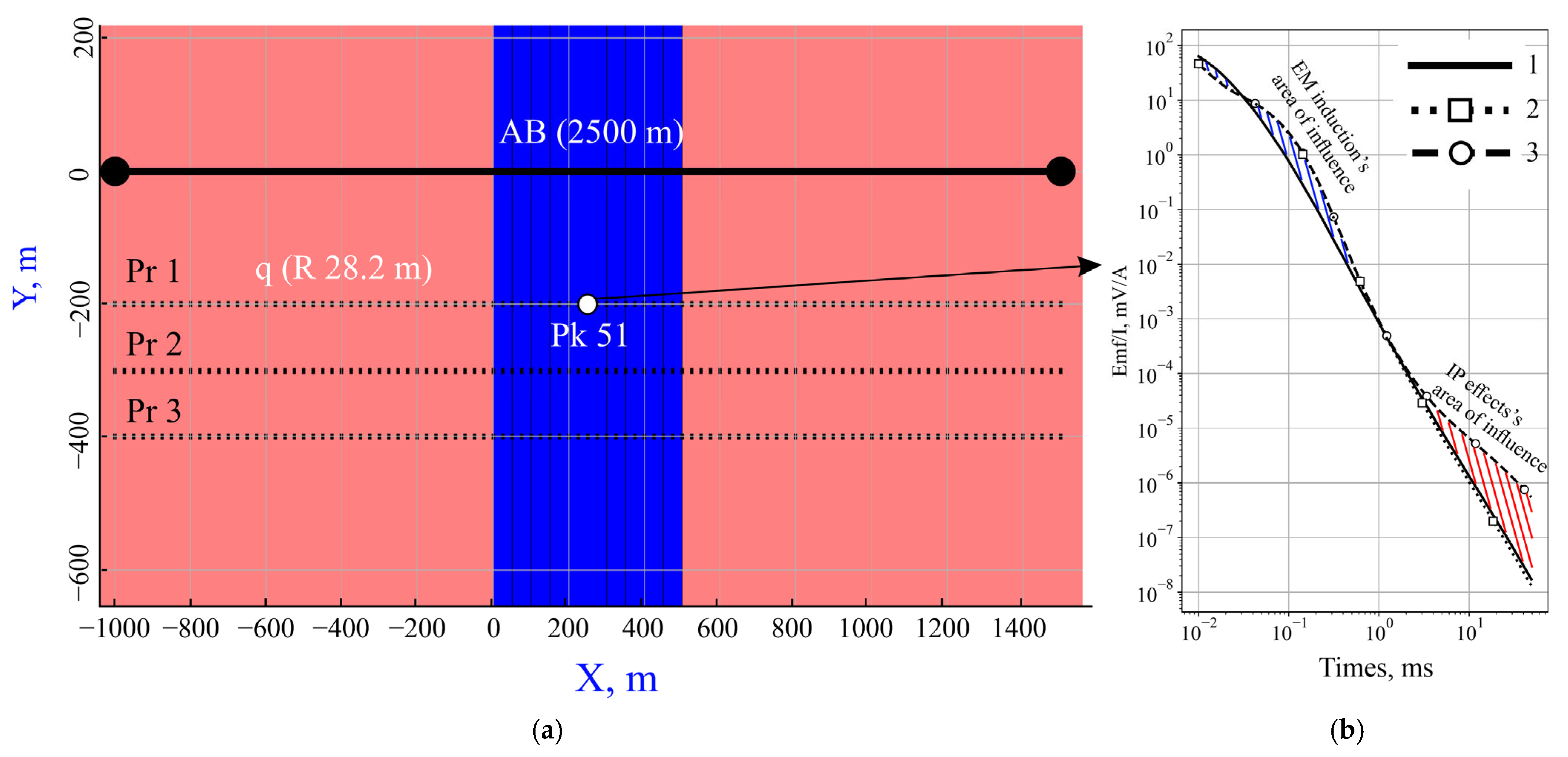
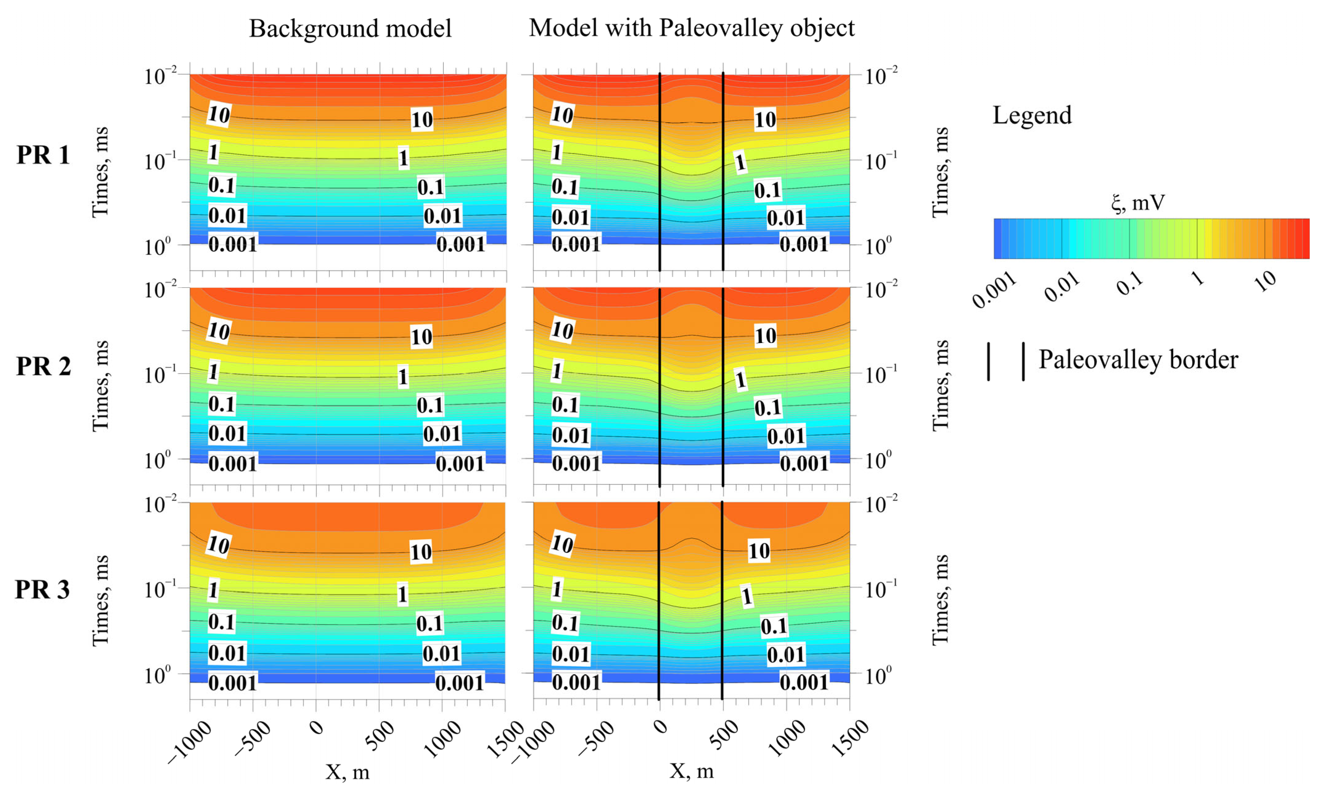
2.5. Numerical Modeling for Sensitivity Assessment

Numerical modeling was carried out in the 3D-inversion program FIEM3D, the direct problem of which was performed on the basis of the finite element method. The mathematical apparatus is described in detail in [29,30]. The electric field strength and magnetic field induction are represented as sums of two components (11) and (12):

$${\overrightarrow{\mathit{E}}}^t={\overrightarrow{\mathit{E}}}^p+{\overrightarrow{\mathit{E}}}^s,$$

(11)

$${\overrightarrow{\mathit{B}}}^t={\overrightarrow{\mathit{B}}}^p+{\overrightarrow{\mathit{B}}}^s,$$

(12)

where ${\overrightarrow{\mathit{E}}}^p$ and ${\overrightarrow{\mathit{B}}}^p$ represent the electric and magnetic primary field strengths and induction in the horizontal-layered medium, and ${\overrightarrow{\mathit{E}}}^s$ and ${\overrightarrow{\mathit{B}}}^s$ are the electric and magnetic strengths and induction determined by the influence of three-dimensional inhomogeneities.

The secondary field, without considering the bias currents, can be found by solving the equation for the vector potential ${\overrightarrow{\mathit{A}}}^s(x,y,z,t)$ [30] (13):

$$\nabla \times \left({\displaystyle \frac{1}{\mu }}\nabla \times {\overrightarrow{\mathit{A}}}^s\right)+\sigma {\displaystyle \frac{\partial {\overrightarrow{\mathit{A}}}^s}{\partial t}}={\sigma \overrightarrow{\mathit{E}}}^p+\nabla \times \left(\left({\displaystyle \frac{1}{{\mu }_0}}-{\displaystyle \frac{1}{\mu }}\right)\nabla \times {\overrightarrow{\mathit{A}}}^p\right),$$

(13)

where $\mu$ is the magnetic permeability of the three-dimensional medium; ${\mu }_0$ is the magnetic permeability of a vacuum; and $\sigma$ is the specific electric conductivity of the three-dimensional medium. The vector potential of ${\overrightarrow{\mathit{A}}}^s$ is related to ${\overrightarrow{\mathit{E}}}^S$ by Relation (14) and to ${\overrightarrow{\mathit{B}}}^s$ by relation (15):

$${\overrightarrow{\mathit{E}}}^S=-{\displaystyle \frac{{\partial \overrightarrow{\mathit{A}}}^s}{\partial t}}$$

(14)

$${\overrightarrow{\mathit{B}}}^S=\nabla \times {\overrightarrow{\mathit{A}}}^s$$

(15)

Similarly, the vector potential of ${\overrightarrow{\mathit{A}}}^p$ is related to ${\overrightarrow{\mathit{E}}}^p$ and ${\overrightarrow{\mathit{B}}}^p$ by the same relations as the vector potential of ${\overrightarrow{\mathit{A}}}^S$ (14) and (15).

The polarization effects are accounted for using the formula for calculating the IP decay (16), which is a recalculation of the Cole–Cole formula for the parameter c = 0.5:

$$\beta \left(t\right)=e^{{\displaystyle \frac{t}{T_0\sqrt{\pi }}}}{\displaystyle \frac{2}{\sqrt{\pi }}}\underset{\sqrt{{\displaystyle \frac{t}{T_0\sqrt{\pi }}}}}{\overset{\mathrm{\infty }}{\int }}{e}^{-x^2}dx,$$

(16)

where $t$ is the delay time after the current is turned off in the generator circuit, and $T_0$ is the decay constant, which is related to the relaxation time τ (from the Cole–Cole formula) through the expression τ = $T_0·\sqrt{\pi }$.

3. Results and Discussion

The geophysical surveys were conducted at the Tetrakh uranium deposit in the Republic of Buryatia (Eastern Transbaikalia, Russia). Figure 4 shows the scheme of the experimental field surveys. The length of line AB was 2.8 km, and the current strength in the AB line was 1.5 A. The UAV was flown at an altitude of 50 m above the digital terrain model, corresponding to an approximate height of 40 m for the measurement sensor. For one second with a pulse and pause duration of 10 ms each, 50 multipolar-sounding curves were recorded. The geologic map (see Figure 4) was made based on a priori data [31]. In the granite of the Vitimkan intrusive complex, Neogene sedimentary deposits are infiltrated beneath a basaltic cover, within which ore-bearing rocks containing varying uranium concentrations are present. Neogene sedimentary deposits overlain by basalts are represented by sediments of the Neogene age that were subsequently covered (and potentially breached) by basaltic cover. Proluvial–deluvial deposits consist of sandstone and sand. The Middle-to-Late Paleozoic granitoids, forming the crystalline basement, are composed of leucocratic and biotite granites.

The survey was carried out at the end of winter in rather difficult weather conditions, at subzero temperatures, and in strong winds, so the data obtained can be considered quite realistic in terms of quality. Thus, the data clearly show the effects of sensor swinging due to gusts of crosswind: due to this, an additional magnetic field was induced on it (the effect of the coil moving in a magnetic field). This led to characteristic distortions of the signal (see Figure 5); the so-called drift appeared when the average value of a pair of multipolar pulses was different from zero.

These effects were eliminated semi-automatically with the help of the primary data processing algorithm, which is described in detail in [16] and, in brief, can be summarized as follows:

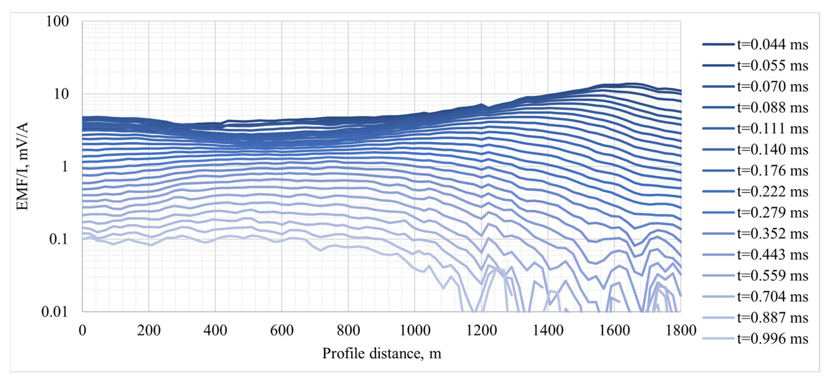
• Extraction is performed from the initial series of sounding curves at current offsets;
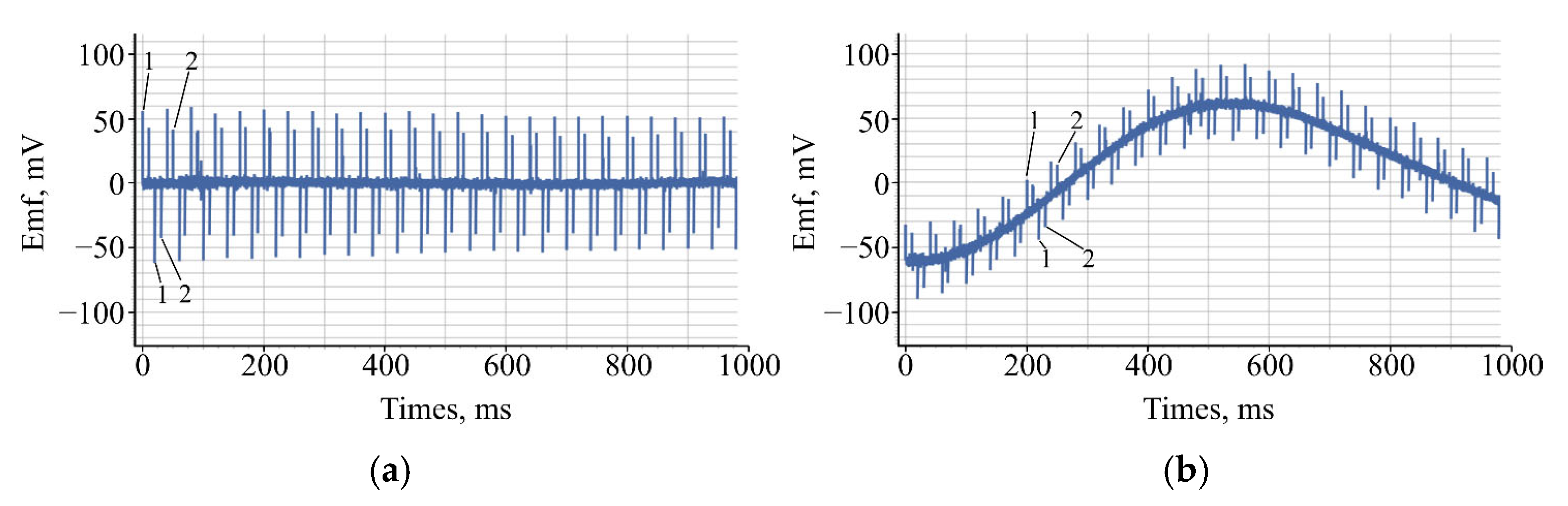
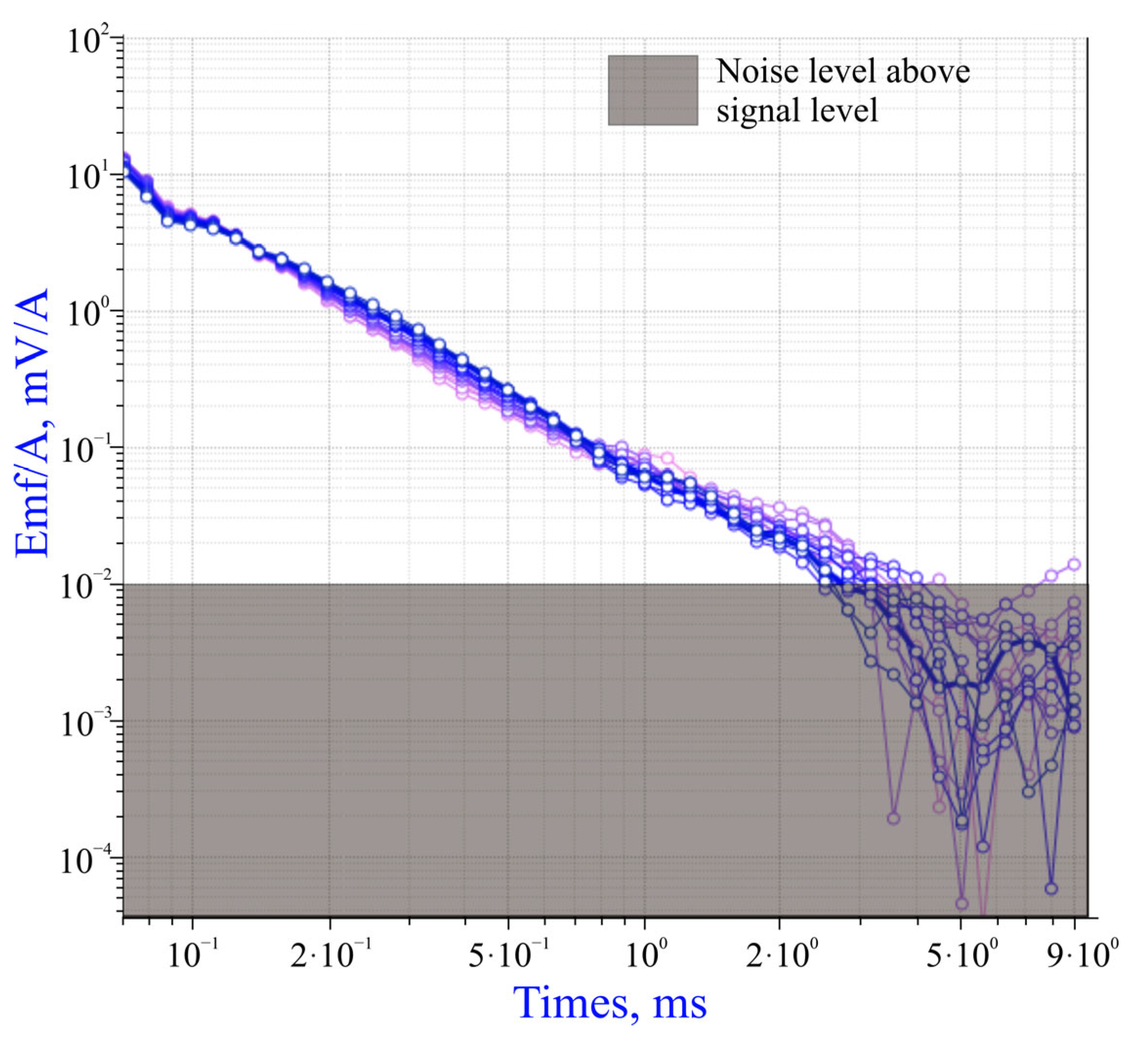
• Drift compensation uses a low-pass filter—this allows distortions like those shown in Figure 5b to be suppressed;
• Robust smoothing using two-dimensional sliding windows is conducted;
• Sounding curves are converted from the arithmetic time step to the logarithmic time step using robust averaging.

Georeferencing each obtained sounding curve is also included in the processing. Thus, probing points are formed, which are used for further inversion.

Below (see Figure 6), the registered current-normalized EMF values over the time series for profile 3 are presented. Lighter line colors indicate later establishment times, up to 1 ms (every second time value is shown in the legend). In the range from 300 to 1000 m along the profile, decreases in EMF are observed at time intervals of 0.1–0.3 ms, which suggests reduced resistivity values in this region. Additionally, at these time intervals, increases in EMF are observed on both sides of the 300–1000 m range, indicating higher resistivity values at approximately the same depths. The rightmost part of the profile (>1100 m profile along) exhibits even higher resistivity: the rate of EMF decline is greater, leading to interference signals appearing at earlier times (up to 1 ms).

The inversion of TEM data was performed within the framework of one-dimensional modeling using the described algorithm. Although polarization parameters were specified in the PGM according to the Cole–Cole formula, no evidence of induced polarization effects was observed in the recorded TDEM curves, as confirmed by the absence of sign reversals in the signals (except for noise at the ends of the curves). The sensitivity assessment of our UAV-TEM system, which will be discussed below, indicates that, in this case, the system was not capable of detecting effects related to induced polarization. Therefore, the solution to the one-dimensional inverse problem was carried out without considering induced polarization effects, simplifying the modeling process and focusing on resistivity variations.

Based on the results of solving the inverse problem for each picket, two sections were constructed along profiles 3 and 4 (Figure 7). The sections show that the effusive basalt strata had resistivity at the level of 700–1500 Ω∙m and were not dissected into separate layers (interlayers of tuffs, interfractional sediments, and lenses of perennially frozen rocks), which was known from drilling data. The paleovalley is distinguished by a conductive area with an average resistivity of about 40–60 Ω∙m at a depth of 120–130 m, which does not contradict the a priori information. The boundaries of the conductive area along profile 3 coincide well with the position of the paleovalley on the right side of the section, but it extends further on the left side, resting on the supposed fault zone. For profile 4, since there is no geologic section, it is not possible to establish the exact position of the paleovalley, but this profile is 100 m away from profile 3, so the position of the paleovalley should not change much. The conductive area on profile 4 extends a little further on the right side of the section, and on the left side, it also rests on a fault zone.

The inconsistencies of the measured and model curves (RMSRE (10)) averaged 4%–7%, but for better convergence of the data, the range of the fitted times varied depending on the quality of the sounding curves (see Figure 8).

In this case, the results of UAV-TEM data inversion within the framework of one-dimensional models are presented. Such an approach to inversion with the software tools available takes quite a long time; for two profiles (3.6 linear km: 161 sounding points), one person worked on this for about two weeks, despite the fact that we are dealing with an area with a fairly simple and clear geological setting and an existing profile 3 with reference drilling data. In conditions where a two-man crew can acquire more than 30 linear kilometers of sounding curves (>1300 sounding points) in one flying workday, inversion with a productivity of about 16 points per man-day is inefficient. One way to resolve this problem has been described previously [17]. However, there is no doubt that the current version of the semi-airborne SibGIS UAV-TEM system, in contrast to earlier versions, now allows an object of the “paleovalley” type to be distinguished quite confidently, and the question of improving the efficiency of this electrical exploration technology as such now lies mainly in the field of developing inversion methods. To confirm this thesis, numerical modeling of the sensitivity of the created system was carried out on the basis of the obtained field data.

An AB-q (“line-loop”) setup (see Figure 9a) was specified with an AB line length of 2500 m and a receiving loop with a radius of 28.2 m (S = 2498.3 m²), which is the equivalent of a square loop with sides of 50 m (S = 2500 m²) or the induction sensor used in reality. The altitude of the loop q above the surface of the medium is given as 40 m. Profiles are set at 200, 300, and 400 m from the side of the transmitter line. On each profile, 101 pickets with a step of 25 m are set. The duration of pulses and pauses is 0.05 s each. Calculations were carried out for a single current, and the shape of the current pulses is ideal (Heaviside function). The time grid is from 0.01 to 45.86 ms. The initial step is 0.001 ms, with a coefficient of 1.12.

Direct problems for all points were calculated in the FIEM3D program twice each. In the first case, the calculation with the above-mentioned object (see Figure 2) was performed, while in the second case, the calculation without 3D objects (only the horizontal layered environment) was taken into account. The theoretical sounding curves calculated from the model with the object in question were calculated without (m = 0) and with polarization effects taken into account (m = 0.2; τ= 0.01 s; c = 0.5).

Examples of model curves in the double logarithmic scale in modulus for the point PK 51 PR 1 are shown in the figure (see Figure 9b). If we consider only the induction contribution (see Figure 9b-1,2), its contribution can be traced up to 0.8 ms, while the effects of induced polarization (IP) start to appear only after 2 ms (see Figure 9b-3) and the signal level is below 10⁻⁴ mV/A. With stationary loops, such signals are quite detectable, but for a towed loop at an altitude of about 40 m, this may not be feasible.

The minimum detectable signal level (sensitivity threshold) for the sensor used was determined based on the results of field experiments. Several curves were plotted along the profile located at a distance of 200 m from the AB line. At a current strength in line AB of 1.5 A, the recorded signal level was 0.01 mV/A (see Figure 10).

Having determined the sensitivity threshold of the TEM system, we can proceed to the analysis of the sounding curves. Pseudo-sections in the form of isosurfaces were constructed from the data of the curves calculated by solving direct problems (see Figure 11). The data were cut off by a time of up to 1 ms because the EMF values at these times exceeded the sensitivity threshold by an order of magnitude. At the edges of the pseudo-sections (X < −500 m and X > 1000 m), especially for the background model, distortions associated with leaving the median gradient zone can be observed. The differences between the background and the sought model are visible to the naked eye; the presence of the target object in the form of a paleovalley distorts the electromagnetic field at early times (see Figure 11).

It is possible to obtain more detailed information about the sensitivity of the UAV-TEM technology to the target object by calculating the anomalous contributions of the target object. The anomalous contribution is calculated for each time delay in two variants: in absolute values (the background theoretical field is subtracted from the theoretical field with the target object (17)) and relative values (as the ratio of the absolute anomalous contribution to the background theoretical field (18)).

$$AAC\left(t\right)={\xi }^{obj}\left(t\right)-{\xi }^{bg}\left(t\right),$$

(17)

$$RAC\left(t\right)={\displaystyle \frac{{\xi }^{obj}\left(t\right)-{\xi }^{bg}\left(t\right),}{{\xi }^{bg}\left(t\right)}}·100\%,$$

(18)

Here, $t$ is time; $AAC\left(t\right)$ is the absolute anomalous contribution at time t; ${\xi }^{obj}\left(t\right)$ is the theoretical EMF calculated for the model with the paleovalley object at time $t$; and ${\xi }^{bg}\left(t\right)$ is the theoretical EMF calculated for the background at time $t$.

Pseudo-sections were plotted from the data of absolute and relative anomalous contributions (see Figure 12). Since the sensitivity threshold was 0.01 mV/A, the absolute anomalous contributions below the threshold value by one order of magnitude in Figure 12 were made transparent. It is noticeable that the anomalous contribution to the electromagnetic field from the target object is spread over the entire profile, which can cause a problem when solving the inverse problem within one-dimensional models. Also, anomalous contributions have alternating functions.

In general, we can conclude that the target object is distinguished in the theoretical sounding curves at times up to 0.5 ms, which falls under the area of influence of EM induction (see Figure 12b); that is, it is not possible to distinguish the paleovalley by the effects of induced polarization, even by increasing the current strength by one order of magnitude (up to 10 A). To register the IP effects in the UAV-TEM data, it is necessary to increase the current strength in line AB by three orders of magnitude (over 1000 A). Taking into account the fact that the upper part of the section of the model and similar ore objects are composed of effusive strata and have high resistivity, it is extremely difficult to supply pulses with current strength in the first thousand amperes to the transmitter line. Thus, at this stage of UAV-TEM technology development, it is impossible to register anomalies caused by polarization processes in this and similar geological situations.

Anomalous signals from three-dimensional heterogeneities extend beyond the boundaries of the object itself in the form of a paleovalley, which is not a novel finding (see Figure 12). At distances of up to 250 m from the object boundary along the profile, the maximum level of the anomalous signal decreases to approximately 1 mV; at 500 m, it diminishes by a factor of 100, reaching about 0.1 mV; and at 1000 m, the values of the anomalous field are slightly above 0.01 mV, while still remaining above our sensitivity threshold. This inevitably impacts the solution of the inverse problem within the framework of one-dimensional models, resulting in an estimated object that appears larger than its actual size. The inversion results confirmed this expectation.

4. Conclusions

As a result of using the SibGIS UAV-TEM semi-airborne technology at a paleovalley-type uranium deposit, TEM sounding curves were obtained, 1D inversion was performed, and the results were compared with drilling data. The paleovalley geometrized based on the results of the UAV geophysical survey coincides well in depth with the available geological data.

A sequence of electrical pulses was induced through a grounded line 2.8 km long with a low current of 1.5 A. A compact receiver with a loop moment of 2500 m², towed by a UAV at a speed of 9–10 m/s at an altitude of 50 m, measured a transient field (∂B_z)/∂t up to 500 μs⁻¹ ms with a frequency of 50 curves per second.

It is shown that the current version of the SibGIS UAV-TEM allows higher-quality sounding curves to be obtained in comparison with those from earlier prototypes [9]. Moreover, it can be argued that the data obtained are now of high quality and are more than sufficient for solving real geological prospecting tasks. Low flight speeds and high-frequency measurements allow very dense measurement networks to be obtained in comparison with both ground surveys and standard EM surveys from helicopters.

Mathematical modeling based on the obtained data shows that the technologies of the semi-airborne UAV-TEM allow the detection and mapping of low-resistance polarizing objects (such as paleovalleys) only by the resistivity parameter, whereas to register the induced polarization it is necessary to increase the current strength above 1000 A, which is impossible in practice.

In general, based on field data and mathematical modeling, it can be concluded that the technology presented in the case is quite effective in identifying the boundary between the basement and the volcanogenic sedimentary cover, mapping conductive zones in granite and other high-resistance rocks at depths of up to several hundred meters, even in a fairly mobile version, with a lightweight, compact current switch and a gasoline generator of low power and weight, which makes it convenient for geological exploration projects in remote areas.

5. Patents

SibGIS Tech LLC.; Parshin, A. Aeroelectric geophysical prospecting method using lightweight unmanned aerial vehicle. RU Patent 2736956 C1, 9 January 2020.

References

1. Dadrass Javan, F.; Samadzadegan, F.; Toosi, A.; van der Meijde, M. Unmanned Aerial Geophysical Remote Sensing: A Systematic Review. Remote Sens. 2024, 17, 110. [Google Scholar] [CrossRef]
2. Parshin, A.V.; Morozov, V.A.; Blinov, A.V.; Kosterev, A.N.; Budyak, A.E. Low-altitude geophysical magnetic prospecting based on multirotor UAV as a promising replacement for traditional ground survey. Geo-Spat. Inf. Sci. 2018, 21, 67–74. [Google Scholar] [CrossRef]
3. Pothuri, R.C.P.; Joseph, C.; Bommu, N.R.; Prabhat, S. Application of UAV-borne Magnetic Survey in Diamond Exploration: A Case Study over Kimberlite-Carbonatite Intrusion from Khaderpet, Eastern Dharwar Craton, South India. J. Geol. Soc. India 2025, 101, 198–207. [Google Scholar] [CrossRef]
4. Accomando, F.; Florio, G. Drone-Borne Magnetic Gradiometry in Archaeological Applications. Sensors 2024, 24, 4270. [Google Scholar] [CrossRef]
5. Shahsavani, H.; Smith, R.S. Aeromagnetic gradiometry with UAV, a case study on small iron ore deposit. Drone Syst. Appl. 2024, 12, 1–9. [Google Scholar] [CrossRef]
6. Molnar, A. Measurement of gamma radiation dose distribution by drone using discrete measurement method. Bull. L.N. Gumilyov Eurasian Natl. Univ. Tech. Sci. Technol. Ser. 2024, 147, 168–187. [Google Scholar] [CrossRef]
7. Parshin, A.; Morozov, V.; Snegirev, N.; Valkova, E.; Shikalenko, F. Advantages of Gamma-Radiometric and Spectrometric Low-Altitude Geophysical Surveys by Unmanned Aerial Systems with Small Scintillation Detectors. Appl. Sci. 2021, 11, 2247. [Google Scholar] [CrossRef]
8. UAV VLF-EM SYSTEM: Resistivity Mapping Solution. Available online: https://www.gemsys.ca/uav-vlf/ (accessed on 18 February 2021).
9. Parshin, A.; Davidenko, Y.; Yakovlev, S.; Vinokurov, V.; Bashkeev, A. Lightweight TEM and VLF systems for low-altitude UAV-based geophysical prospecting. In Proceedings of the NSG2021 27th European Meeting of Environmental and Engineering Geophysics Conference Proceedings, Bordeaux, France, 2 September 2021; Volume 2021, pp. 1–5. [Google Scholar]
10. Kotowski, P.O.; Becken, M.; Thiede, A.; Schmidt, V.; Schmalzl, J.; Ueding, S.; Klingen, S. Evaluation of a Semi-Airborne Electromagnetic Survey Based on a Multicopter Aircraft System. Geosciences 2022, 12, 26. [Google Scholar] [CrossRef]
11. Stoll, J.; Noellenburg, R.; Kordes, T.; Becken, M.; Tezkan, B.; Yogeshwar, P.; Bergers, R.; Matzander, U. Semi-Airborne electromagnetics using a multicopter. In Proceedings of the International Workshop on Gravity, Electrical & Magnetic Methods and Their Applications, Xi’an, China, 19–22 May 2019. [Google Scholar]
12. Vilhelmsen, T.B.; Døssing, A. Drone-towed controlled-source electromagnetic (CSEM) system for near-surface geophysical prospecting: On instrument noise, temperature drift, transmission frequency, and survey set-up. Geosci. Instrum. Methods Data Syst. 2022, 11, 435–450. [Google Scholar] [CrossRef]
13. Becken, M.; Nittinger, C.G.; Smirnova, M.; Steuer, A.; Martin, T.; Petersen, H.; Meyer, U.; Mörbe, W.; Yogeshwar, P.; Tezkan, B.; et al. DESMEX: A novel system development for semi-airborne electromagnetic exploration. Geophysics 2020, 85, 253–267. [Google Scholar] [CrossRef]
14. Günther, T.; Ronczka, M.; Rochlitz, R.; Müller-Petke, M. Using Drone-Based Electromagnetics for 3D Imaging of Groundwater Salinization. European Association of Geoscientists & Engineers. In Proceedings of the NSG2022 3rd Conference on Airborne, Drone and Robotic Geophysics, Belgrade, Serbia, 18–22 September 2022; Volume 2022, pp. 1–5. [Google Scholar] [CrossRef]
15. Smit, J.P.; Stettler, E.H.; Price, A.B.W.; Schaefer, M.O.; Schodlok, M.C.; Zhang, R. Use of drones in acquiring B-feld total-feld electromagnetic data for mineral exploration. Miner. Econ. 2022, 35, 455–465. [Google Scholar] [CrossRef]
16. Parshin, A.; Bashkeev, A.; Davidenko, Y.; Persova, M.; Iakovlev, S.; Bukhalov, S.; Grebenkin, N.; Tokareva, M. Lightweight Unmanned Aerial System for Time-Domain Electromagnetic Prospecting—The Next Stage in Ap-plied UAV-Geophysics. Appl. Sci. 2021, 11, 2060. [Google Scholar] [CrossRef]
17. Davidenko, Y.; Hallbauer-Zadorozhnaya, V.; Bashkeev, A.; Parshin, A. Semi-Airborne UAV-TEM Sys-tem Data Inversion with S-Plane Method—Case Study over Lake Baikal. Remote Sens. 2023, 15, 5310. [Google Scholar] [CrossRef]
18. Wu, J.; Xiao, D.; Du, B.; Liu, Y.; Zhi, Q.; Wang, X.; Deng, X.; Chen, X.; Zhao, Y.; Huang, Y. Exploring Shallow Geological Structures in Landslides Using the Semi-Airborne Transient Electromagnetic Method. Remote Sens. 2024, 16, 3186. [Google Scholar] [CrossRef]
19. Sun, H.; Zhang, N.; Li, D.; Liu, S.; Ye, Q. The first semi-airborne transient electromagnetic survey for tunnel investigation in very complex terrain areas. Tunn. Undergr. Space Technol. 2023, 132, 104893, ISSN 0886-7798. [Google Scholar] [CrossRef]
20. Tarkhanova, G.A.; Prokhorov, D.A. Genetic features of “Vitim” type uranium ore formation. Razved. I Ohr. Nedr = Prospect Miner. Resour. 2017, 11, 47–59. (In Russian) [Google Scholar]
21. Federal Agency for Subsoil, Federal State Unitary Enterprise All-Russian Scientific Research Institute of Mineral Resources. Geological and Industrial Types of Uranium Deposits in the CIS Countries; VIMS: Moscow, Russia, 2008; 72p, ISBN 978-5-901837-43-6. (In Russian) [Google Scholar]
22. Cole, K.S.; Cole, R.H. Dispersion and absorption in dielectrics. Alternating current characteristics. J. Chem. Phys 1941, 9, 341–351. [Google Scholar] [CrossRef]
23. Pelton, W.H.; Ward, S.H.; Hallof, P.G.; Sill, W.R.; Nelson, P.H. Mineral discrimination and removal of inductive coupling with multifrequency IP. Geophysics 1978, 43, 588–609. [Google Scholar] [CrossRef]
24. Zaharkin, A.K. Compact receiving loop for pulsed electrical prospecting. Ross. Geofiz. Zhurnal Russ. Geophys. J. 1998, 9–10, 95–99. (In Russian) [Google Scholar]
25. Hampel, F.R.; Ronchetti, E.M.; Rousseeuw, P.J.; Stahel, W.A. Robust Statistics: The Approach Based on Influence Functions; John Wiley & Sons, Inc.: New York, NY, USA, 1986; 502p. [Google Scholar]
26. Pushkarev, P.Y.; Yakovlev, A.G.; Yakovlev, A.D. Program for Solving the Direct and Inverse One-Dimensional Problem of the Frequency Sounding Method; Moskow State University: Moscow, Russia, 1999; 12p, Available online: https://spectra-geo.narod.ru/Publications/msu_fs1d.pdf (accessed on 18 February 2021). (In Russian)
27. Ryzhov, A.A. Optimal algorithm for solving the direct VES problem. Fiz. Zemli Izv. Phys-Ics Solid Earth 1983, 3, 68–75. [Google Scholar]
28. Gegenfurtner, K.R. PRAXIS: Brent’s algorithm for function minimization. Behavior Research Meth-ods. Instrum. Comput. 1992, 24, 560–564. [Google Scholar] [CrossRef]
29. Soloveichik, Y.G.; Persova, M.G.; Domnikov, P.A.; Koshkina, Y.I.; Vagin, D.V. Finite element solution to multidimensional multisource electromagnetic problems in the frequency domain using non-conforming meshes. Geophys. J. Int. 2018, 212, 2159–2193. [Google Scholar] [CrossRef]
30. Persova, M.; Soloveichik, Y.; Vagin, D.; Kiselev, D.; Kondratyev, N.; Koshkina, Y.; Trubacheva, O. Application of non-conforming meshes with hexahedral cells for3D modelling of airborne electro-magnetic technologies. Dokl. Akad. Nauk Vyss. Shkoly Ross. Fed. Proceed-Ings Russ. High. Sch. Acad. Sci. 2018, 1, 64–79. (In Russian) [Google Scholar] [CrossRef]
31. Ovsyannikova, T.; Grebenkin, N.; Mashnin, D.; Nesmeyanova, A.; Prokhorov, D.; Starodubov, A.; Tuboltsev, I. Cases and practices of implementing isotopic geochemical methods in search for consealed uranium deposites. Razved. I Ohr. Nedr Prospect. Miner. Resour. 2022, 8, 53–63. (In Russian) [Google Scholar] [CrossRef]
Figure 1. Generalized geological section of Vitim-type paleovalley-related deposits.
Minerals 15 00630 g001
Figure 2. Physical–geological model of the Vitim-type uranium deposit: (a) cross-section; (b) plan view.
Minerals 15 00630 g002
Figure 3. UAV with measuring system (a); KER-100 current switch (b); transmitter line groundings (c); principal flight scheme (d); and measuring unit/ADC (e).
Minerals 15 00630 g003aMinerals 15 00630 g003b
Figure 4. The transmitter line and survey profiles on the geologic map.
Minerals 15 00630 g004
Figure 5. An example of a raw signal sequence without swing (a) and with swing (b) for the receiving loop. 1. The pulse in the receiving loop when switching on the current in line AB. 2. The pulse when switching off the current in line AB.
Minerals 15 00630 g005
Figure 6. TDEM data along the survey line (profile 3), displaying EMF at different times on a logarithmic scale. The time gates are color-coded: early times are shown in dark blue, and late times are shown in light blue.
Minerals 15 00630 g006
Figure 7. Results of solving the inverse problem. (a) Resistivity section along profiles 3 and 4; (b) Results of geological interpretation of data for profile 3.
Minerals 15 00630 g007
Figure 8. Example of the fitting TEM curves for several pickets at profile 3.
Minerals 15 00630 g008
Figure 9. The layout of survey line (a) and theoretical TEM curves calculated from the model (b): 1 background; 2 a paleovalley model (EM only); and 3 a paleovalley model (taking into account the IP).
Minerals 15 00630 g009
Figure 10. Observed TEM curves received by the sensor at an altitude of ~47 m and a distance of 200 m from the AB line.
Minerals 15 00630 g010
Figure 11. Pseudo-sections of theoretical TEM curves for the background model (1D) and paleovalley’s model (3D) for three profiles.
Minerals 15 00630 g011
Figure 12. Pseudosections of anomalous contributions: (a) absolute; (b) relative.
Minerals 15 00630 g012