A Case History of Graphite Exploration in North Norway Integrating Various Geophysical Surveys

Abstract

Graphite is considered to be one of Europe’s most critical minerals. It is necessary for the transition from hydrocarbon fuel to electricity due to its use in batteries that power electronic devices and electric transport. In the past, high-quality exposed graphite was found in Norway without today’s advanced geophysical and geological methods. Norway is a key destination in Europe for graphite production. With an increasing demand for graphite, there have been efforts to systematically survey the country using modern geophysical and geological methods to find hidden graphite deposits. Among the various geophysical survey methods, electrical and electromagnetic (EM) methods are the first choice for the exploration of graphite due to the material’s high electrical conductivity. Airborne surveys are often used to cover a large area for a regional reconnaissance survey to locate the sites with potential mineral deposits before performing ground geophysical and geological surveys. Therefore, frequency-domain helicopter EM (HEM) and airborne magnetic surveys were performed in Northern Norway to locate interesting anomalies which were followed by ground surveys such as electrical resistivity tomography (ERT), charged-potential (CP), self-potential (SP), ground EM, and geological surveys. Some locations were also investigated with drilling and petrophysical core-sample analysis. In this paper, we present helicopter EM and magnetic data, 3D inversion of HEM data, and a successful ground follow-up survey result from the Vesterålen district in Northern Norway. The HEM survey identified previously known and new graphite occurrences, both partially exposed or buried, which were confirmed using ground surveys, drilling, and laboratory analysis of the samples.

1. Introduction

Graphite is a crucial material that is used in batteries that power portable electronic devices and cars as well as in high-temperature lubricants. The transition from hydrocarbon fuel to electrical energy will result in a significant increase in the demand for graphite [1,2,3]. Graphite is a common mineral found in the Norwegian metasedimentary bedrock. However, only a few deposits are exposed to the surface as flake graphite deposits, which are not of economic importance [4]. All Norwegian graphite is of sedimentary origin; however, hydrothermal processes during subsequent stages of high-degree metamorphism have also contributed to its formation [5].

Norway has been a major graphite producer for over 100 years [6]. There are more than 70 registered graphite occurrences located in four graphite provinces in Norway (Figure 1). Most of the registered occurrences were poorly exposed on the surface; therefore, detailed geological and geophysical investigations were necessary to determine their size and depth, confirm their mineral prospective value, and find new deposits. The Skaland graphite mine on the island of Senja is the only deposit that is still in operation, producing ca. 10,000 tons per year. There are currently no active graphite mines in the other provinces [7].

In the early fifties, all the known graphite occurrences in Northern Norway were investigated as co-occurrences with uranium [8]. Later, in the nineties, exploratory activities were conducted to look for graphite resources in Vesterålen [9]. In 1988, an airborne geophysical survey was conducted over a part of Langøya in Vesterålen [10]; however, only part of this survey involved electromagnetic (EM) measurements. From 1990–1994, graphite occurrences in the Jennestad area were reinvestigated using sampling, drilling, and ground geophysics and a total of 1100 m of drilling was performed on 15 different drill holes. In the Hornvann area, proven reserves of 240,000 tons with a grade of 25% graphitic carbon (Cg) were mapped [9,11].

In 2011, new airborne geophysical surveys for general bedrock mapping in the Vesterålen area were performed as part of the mineral resources in Northern Norway (MINN) project at NGU [12]. Based on helicopter-borne geophysics, a systematic follow-up study including various ground-based geophysical and geological surveys was performed between 2015 and 2019 to delineate the graphite deposits in the area [7]. These geophysical surveys and follow-up work led to the discovery of many new graphite mineralization sites. Part of the work was published in [5,6,13,14].

Graphite is an electrically conductive and diamagnetic mineral; therefore, it can be explored using electrical, EM, and magnetic methods [15,16]. Electrical resistivity tomography (ERT), induced polarization (IP), and self-potential (SP) surveys are other geophysical methods that have been successfully used in the exploration of graphite [17,18].

This paper describes recent work in the last few years focusing on geophysical surveys [4], including helicopter-borne EM (HEM), helicopter-borne magnetic and ground-based ERT, IP, SP, and charged-potential (CP), as well as ground EM geophysical methods for locating exposed and non-exposed graphite deposits. We also carried out advanced 3D inversion of HEM and helicopter-borne magnetic data at some of the deposits in the Vesterålen region, North Norway. The main aim of integrating various geophysical methods is to confirm the presence of conductive materials in the subsurface and distinguish graphite deposits from other conductive materials (e.g., saltwater-filled fractures and weathered zones) using various geophysical and geological follow-up surveys.

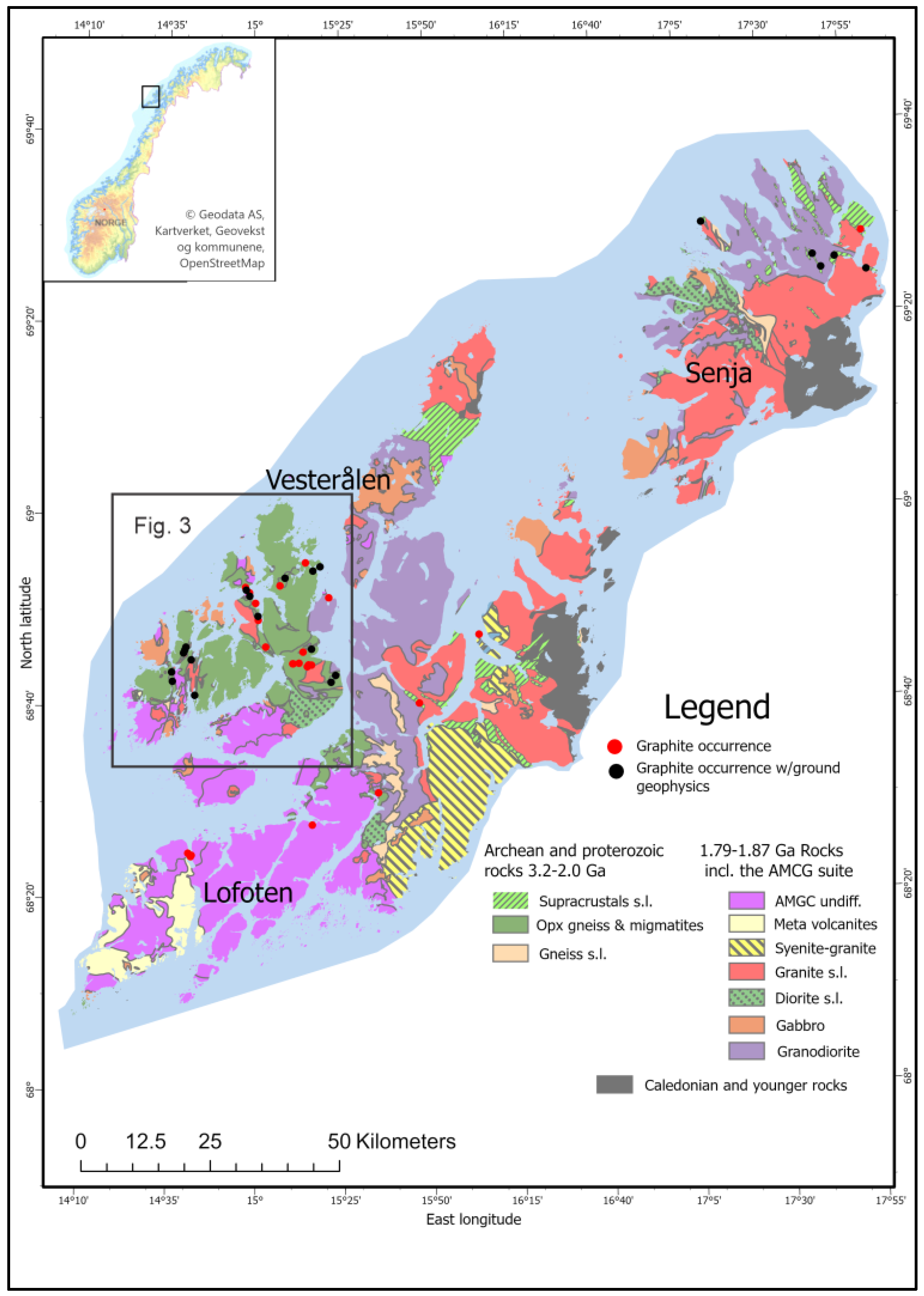
2. Geological Setting

Parnell et al. [19] highlighted that more than 80% of the world’s major graphite deposits can be traced back to paleoproterozoic rocks formed about 2.0–2.2 Ga. Paleoproterozoic graphite is found on every continent and in abundance with high-grade graphite deposits containing high levels of total carbon in the Baltic (Fennoscandian) Shield stretching across Norway, Sweden, Finland, and Russia. We focus on graphite mapping in Northern Norway, specifically the Vesterålen province where > 50 occurrences have been found. The graphite-bearing rocks in Vesterålen occur in sequences belonging to a precambrian domain comprising Lofoten, Vesterålen, and the western islands of Troms County (Figure 2).

The general geology of these areas was studied and outlined by Heier [20], Griffin et al. [21], and Laurent et al. [22]. In general, the area is composed of an archaean to possibly early proterozoic basement of magmatic and metasedimentary rocks, intruded by an early proterozoic magmatic suite composed of anorthosite–mangerite–charnockite–granite (AMCG) rocks. The tectono-magmatic and structural history of Senja, Lofoten, and Vesterålen and their correlation with other parts of the Fennoscandian Shield was reviewed by Bergh et al. [23]. Heier [20] and Griffin et al. [21] described a westward increase in the metamorphic gradient, from amphibolite facies in the east to high granulite facies in the west in the Lofoten–Vesterålen area. Olesen et al. [24] described the petrophysical details of this transition, which contains most of the high-quality coarse flake graphite occurrences present within granulite facies areas.

3. Materials and Methods

Graphite deposits can be distinguished from other conducting materials, e.g., seawater, saltwater-filled fractures, and weathered zones, using induced polarization (IP) surveys [25]. In a porous medium (with ionic conduction), electrically conductive minerals such as graphite (with electronic conduction) will act as a capacitor and produce an IP effect while conductive saltwater-bearing rocks, which only produce ionic conduction, will have no IP effect. Massive graphite deposits will only produce an IP effect at the edges because of continuous internal electronic conduction and accumulation of the charges at the contacts. Clay deposits also display some IP effects; however, they are not as strong as those produced by disseminated graphite. A self-potential (SP) survey is another useful method which can identify high SP anomalies due to graphite mineralization. This study used HEM, helicopter magnetic, ERT, IP, CP, SP, and ground EM (using EM31) geophysical methods. Samples from trenches and cores were analyzed for petrophysical properties and total carbon content to confirm the presence of graphite. Some drill holes were also logged to confirm the presence of graphite at different depths.

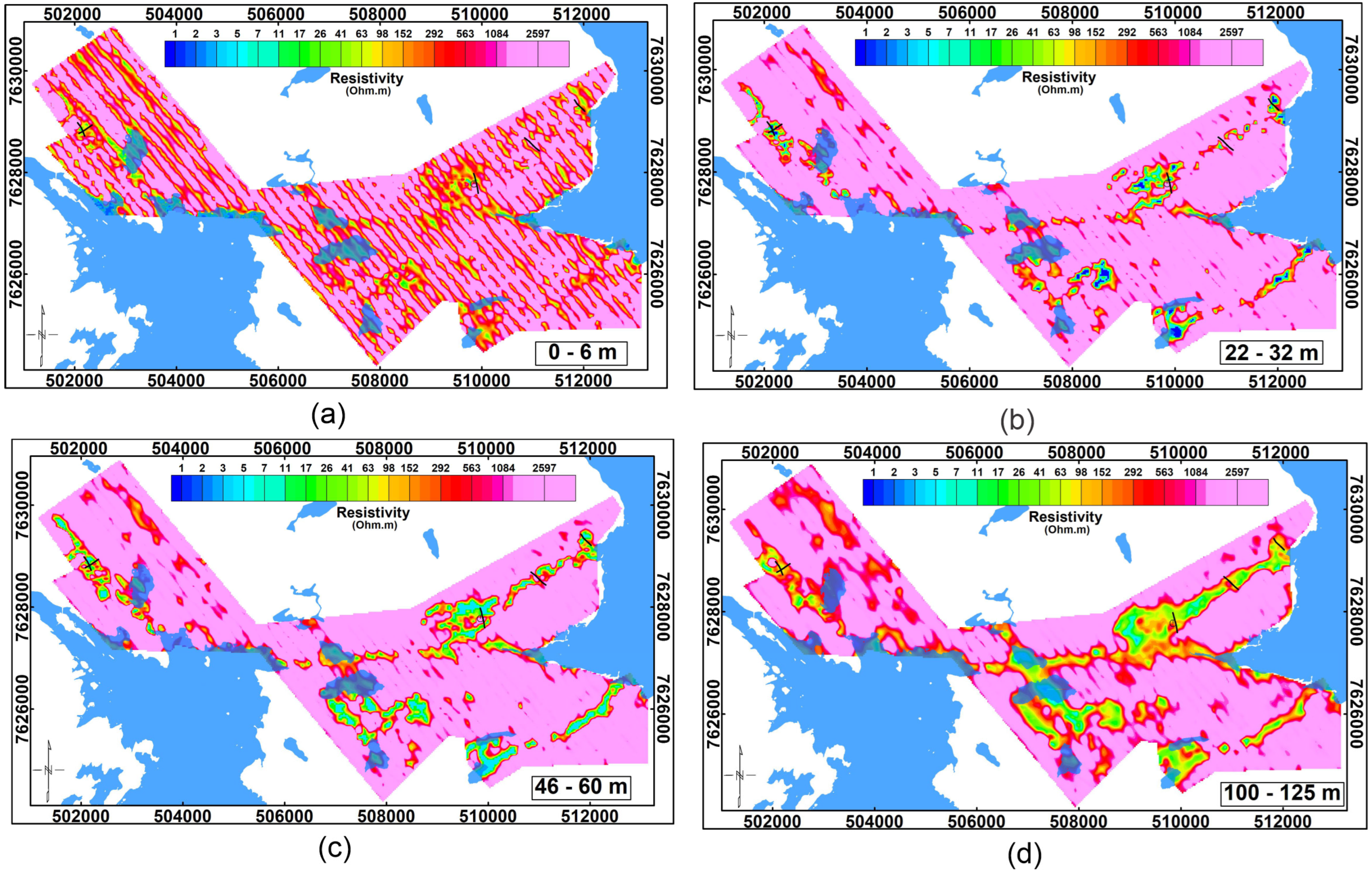
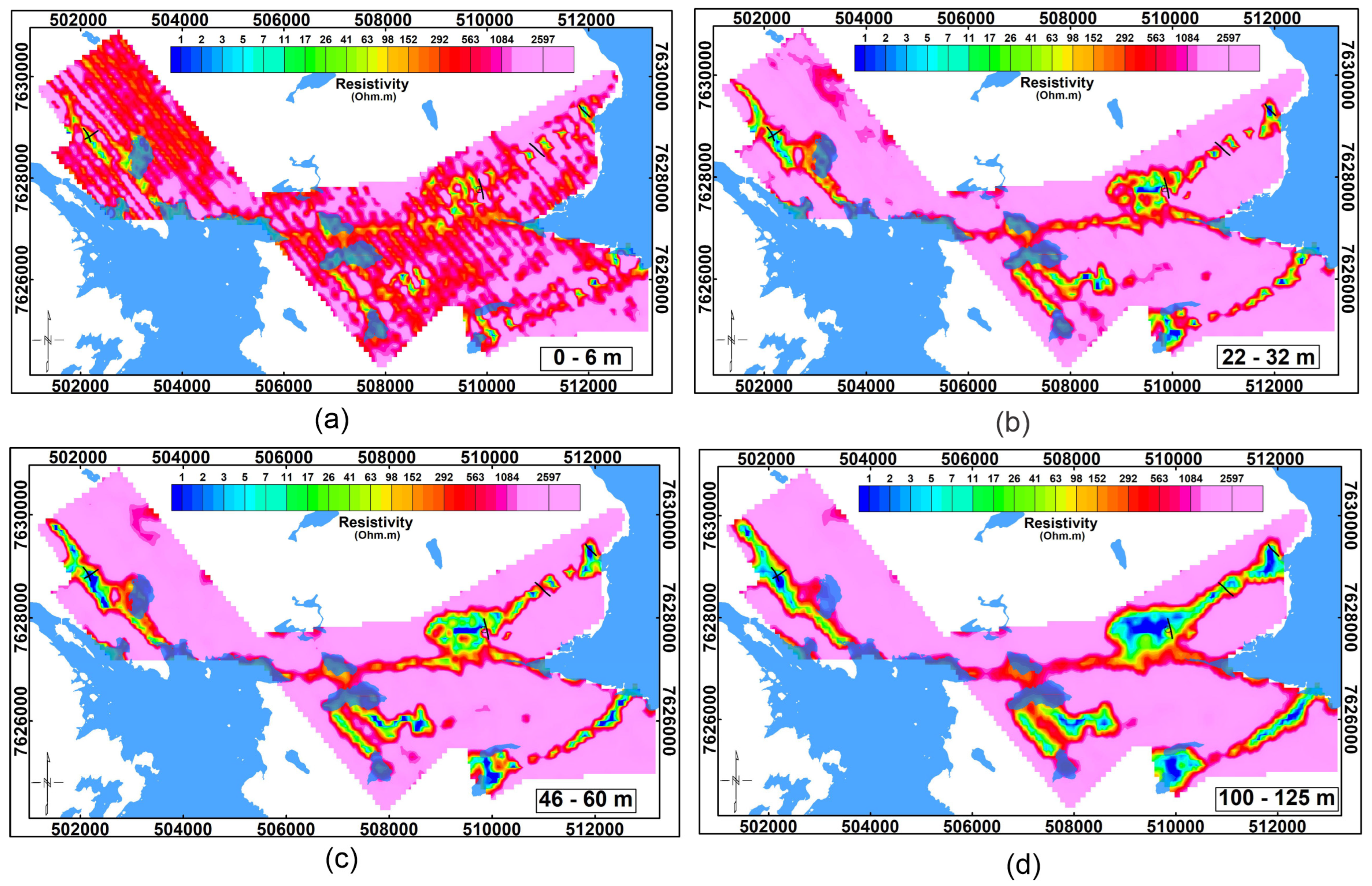
3.1. Helicopter-Borne Electromagnetic and Magnetic Method

The Geological Survey of Norway (NGU) has a five-frequency HEM system which is a modified Geotech hummingbird system. Primary EM signals are transmitted at five frequencies through five different transmitter coils corresponding to five receiver coils that are used to measure in-phase and quadrature components of the induced secondary EM fields from the Earth. Three frequencies, 880, 6606, and 34,133 Hz, operate in the coplanar setting and two frequencies, 980 and 7001 Hz, operate in the coaxial setting of the transmitter and receiver coils. All five transmitter–receiver coil systems are held together with a bucking coil and are housed in a 7 m long bird that is towed 30 m below the helicopter. The bird also has an optical-pumped cesium magnetometer which records the natural magnetic fields of the Earth together with the HEM measurements. Generally, gamma-ray spectrometry data are also recorded at the same time using a gamma-ray spectrometer installed under the belly of the helicopter; however, previous work has found that gamma-ray spectrometry data are not useful for graphite exploration.

The helicopter-borne geophysical survey was carried out at Langøya, Vesterålen in Northern Norway in 2013 (red rectangle in Figure 2), covering an area of 1050 km² (i.e., 5650 line-km) with a flight line spacing of ca. 200 m in the E–W direction at ca. 60–70 m altitude. The helicopter was lifted to ca. 1000 m altitude every 20 min of flying to measure a nulling position for all the HEM receivers, assuming that there was no signal observed from the ground at this height. These nulling positions were used to correct the drift in the HEM signals. Drift in HEM signals is commonly observed due to temperature variation in the electronics of the HEM system during flying and must be corrected to make sure that the signals received are due to ground conductivity variations and not instrumental drift or other external factors. HEM data were processed using 20-point low-pass and 3-point high-pass filters and manual editing to remove cultural noises. Instrumental drift was removed using the high-altitude flights. Technical details of the survey, acquisition, and data processing can be found in Rodionov et al. [12]. Apparent resistivity was calculated from processed in-phase and quadrature data at all five frequencies of the HEM survey using a 1000 Ωm starting model and half-space inversion method [26]. The noise floor for the half-space inversion was assumed to be 5 ppm at high frequencies (34,133, 7001, and 6606 Hz) and 3 ppm at low frequencies (980 and 880 Hz). The highest frequency (34,133 Hz) data contain information from the shallow subsurface (ca. 0–20 m below the ground) conductors and the lowest frequency (880 Hz) data contain information from deeper (ca. 100 m below the ground) conductors. Total magnetic field anomaly was calculated from the magnetic field after diurnal and international georeferenced magnetic field (IGRF) correction.

3.2. Ground Electromagnetic Measurements

Based on the same principle of EM induction as HEM, a ground conductivity meter, e.g., modified Geonics EM31 [27], was used to map known and unknown nearly outcropping graphite deposits. This instrument is calibrated such that it measures the apparent electrical conductivity directly in mS/m down to 7–10 m. The instrument has horizontal coplanar coils separated by 3.8 m and works at a frequency of 9800 Hz. NGU modified this instrument in 2017, adding a GPS positioning system, magnetic sensor, and data acquisition system.

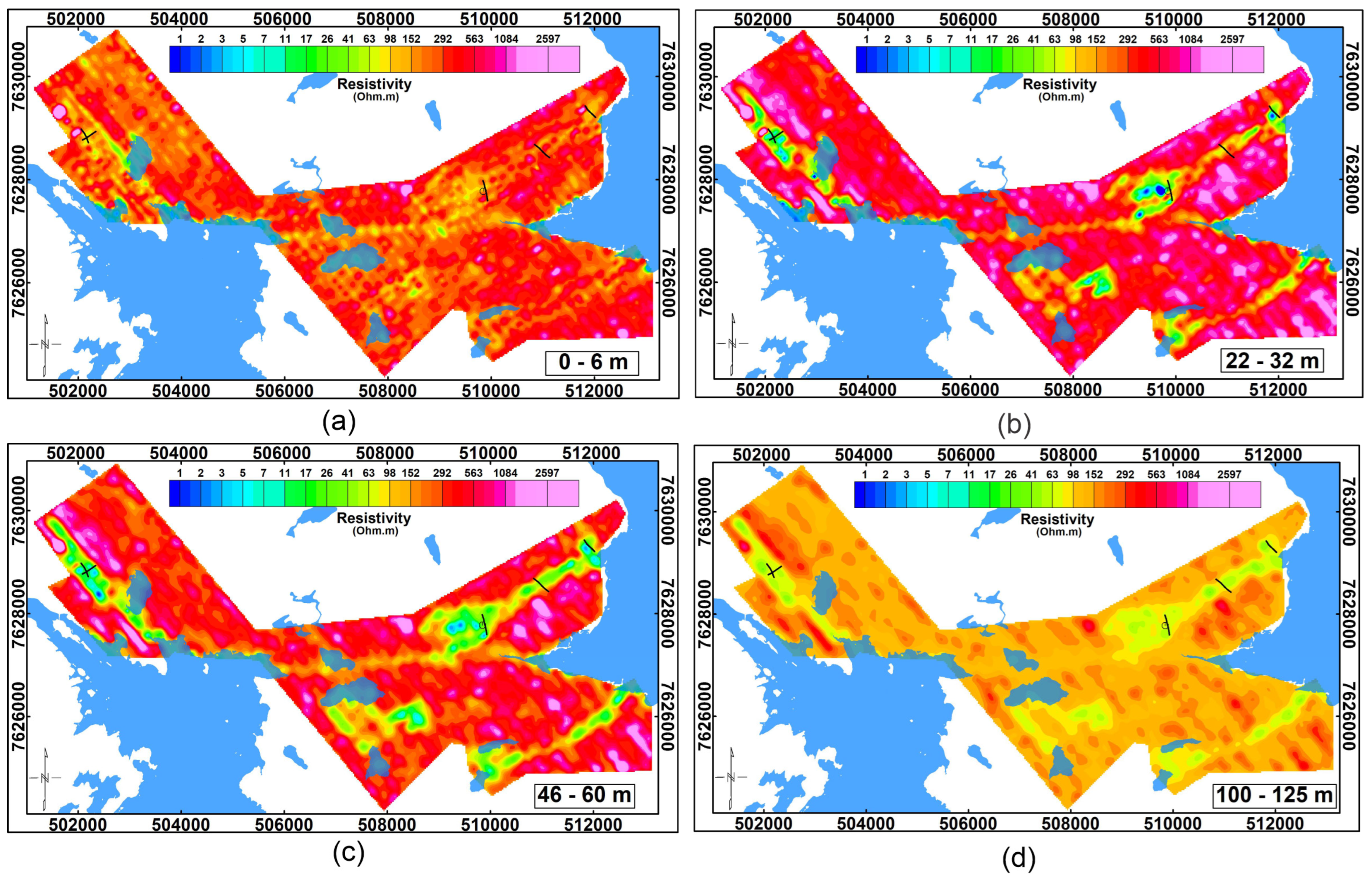
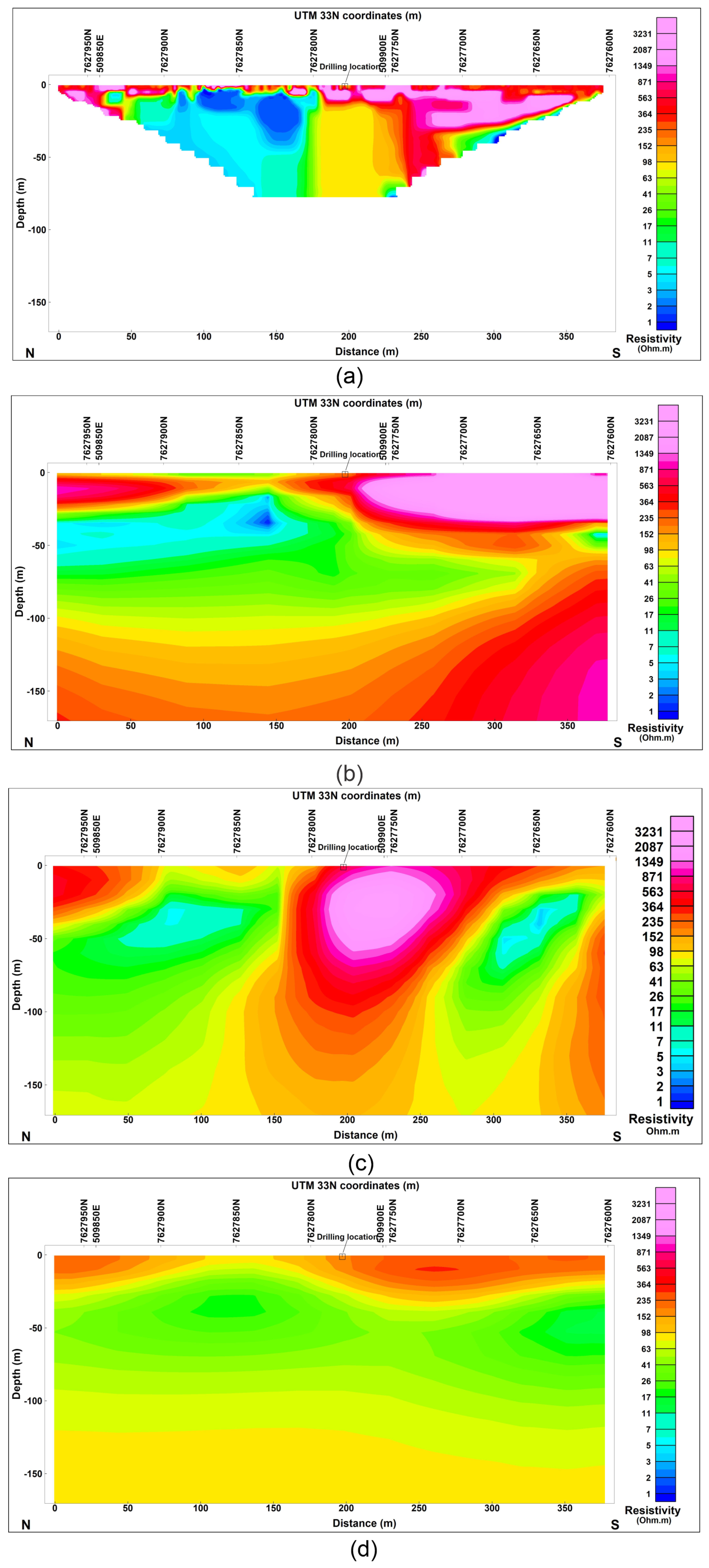
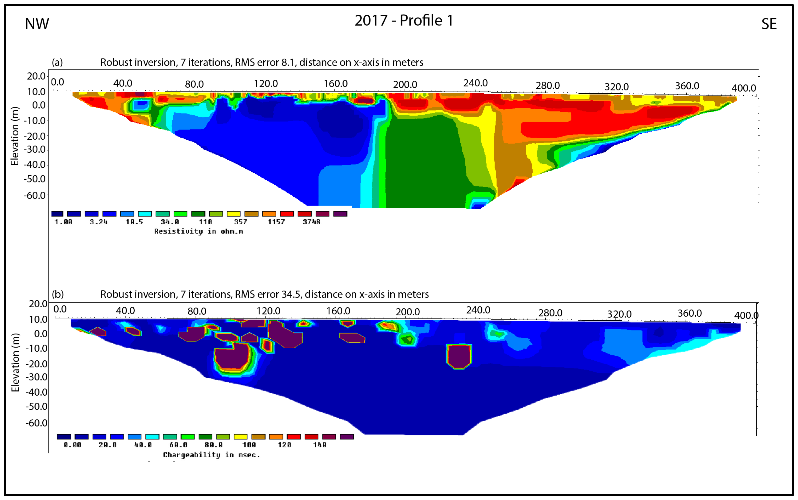
3.3. Electrical Resistivity Tomography (ERT) and Induced Polarization (IP)

The 2D resistivity or ERT and IP methods are carried out by injecting current into the ground using two current electrodes and by measuring the voltage difference between four pairs of separated potential electrodes. Based on measured resistance (i.e., measured voltage/injected current) and a geometrical factor depending on the electrode positions, the apparent resistivity and IP effect of the subsurface can be calculated. The 2D resistivity/IP measurements were performed using the Lund cable system [28], ABEM Terrameter LS instrument [29], and multiple gradient electrode configurations [30]. An automatic measuring procedure generates current at one electrode pair and measures the electric potential of up to four electrode pairs simultaneously after the electrodes are connected to the ground and the measuring instrument. Resistivity is measured when the current is on while the IP effect is measured shortly after the current is stopped. An electrode separation of 5 m was used for the profiles, giving a maximum depth range of about 60 m as a compromise between depth penetration and resolution [31].

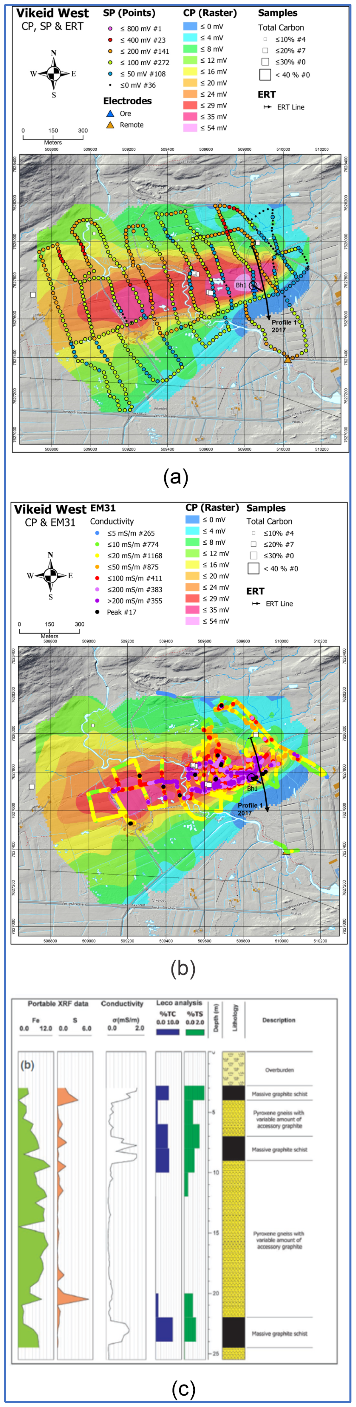
3.4. Charged-Potential (CP) and Self-Potential (SP) Measurements

In 2014, NGU developed the equipment used for combined CP and SP measurements which consists of an immobile current transmitter and a mobile receiver (voltmeter). The details of the instrumentation and measuring strategy can be found in Rønning et al. [4].

CP measurements are acquired by connecting a current electrode directly to the conductive body and locating the other remote electrode at a considerable distance so that its effect is virtually non-existent in the survey area. By measuring the potential above and around the known graphite ore body, the body’s strike, strike length, dip, and length along the dip can be mapped. In addition, an outline of unknown ore bodies in the neighboring area can be mapped. A practical way of interpreting the depth extent of nearly vertical conductive bodies from CP data is presented in Kihle and Eidsvig [32].

SP is a natural potential observed in the ground. It is created by electrochemical processes in adjacent electronic conductors such as graphite, sulfides, and oxides [33]. It is measured simultaneously with CP and is not dependent on exposed graphite for current injection. It is a useful tool if several conductive bodies are present in the investigated area. It may produce negative potential values ≥ 1000 mV above graphite mineralization. SP signals < 50 mV are not regarded as significant anomalies in mineral prospecting.

3.5. Analytical Methods

Most of the investigated area is partly covered in soil; however, there are numerous outcrops, particularly on the mountain tops. The graphite schist found in these areas was sampled in order to obtain as many representative samples as possible from as large an area as possible. These samples were analyzed at the NGU laboratory for various chemical elements [4]. Powdered samples were analyzed for total carbon (TC) and total sulfur (TS) using a Leco SC-632 analyzer which can detect levels of carbon and sulfur as low as 0.06% and 0.02%, respectively.

3.6. Core Drilling, Sampling, and Analyses

Areas of high electrical conductivity were drilled, and the boreholes were logged using a simple drill-hole resistivity probe, ABEM SAS-LOG 200 [34]. The drill core was geologically logged, sampled, analyzed, and reported as follows: (1) Lithological logs and descriptions of cores; (2) Dry and wet photographs; (3) Portable XRF measurements at 0.25 m intervals. The most graphite-rich intervals were analyzed for TC and TS.

4. Results

We present here only the HEM and helicopter magnetic data that are relevant to graphite exploration. All the data from the helicopter surveys in Norway can be downloaded from the NGU website as jpg maps or georeferenced data sets (geotiff files). Apparent resistivity measurements at different frequencies were quite similar [12] for this area; therefore, we show the results for only one apparent resistivity, 7 kHz (Figure 3a). Low resistivity areas on the apparent resistivity image (purple to yellow colors in Figure 3a) show conductive minerals, seawater, saltwater-filled fractures, and weathered bedrock. Magnetic anomaly after reduction to the pole (RTP) is shown in Figure 3b. A geomagnetic inclination of 77.7 and geomagnetic declination of 5.1 were used for reduction to the pole. Low magnetic anomaly is generated due to the absence of magnetic materials in the rock, remanent magnetization, and the diamagnetic nature of graphite. We observed a correlation between low magnetic anomaly and low apparent resistivity at the locations of known and exposed graphite (black symbols in Figure 4). This correlation is shown more clearly by zooming into a small area (black and red squares area in Figure 3a,b) and later in Figure 5b,c. We combined magnetic anomalies < 300 nT and apparent resistivity < 300 Ωm together into a single anomalous zone to identify probable graphite-containing locations (Figure 4) for further ground geophysical and geological follow-up work.

Figure 3. (a) Apparent resistivity image from 7 kHz frequency HEM data and (b) magnetic anomaly with flight lines. The black rectangular area is enlarged in Figure 5 to show topographic variation and the correlation between low apparent resistivity and low magnetic anomaly.

Figure 3. (a) Apparent resistivity image from 7 kHz frequency HEM data and (b) magnetic anomaly with flight lines. The black rectangular area is enlarged in Figure 5 to show topographic variation and the correlation between low apparent resistivity and low magnetic anomaly.

Figure 4. Graphite prospecting map based on the correlation between apparent resistivity < 300 Ωm and < 300 nT magnetic anomaly. Exposed graphite locations known prior to (black squares) and after airborne survey (red squares) are marked. The black rectangular area is enlarged in Figure 5 to show topographic variation and the correlation between low apparent resistivity and low magnetic anomaly.

Figure 4. Graphite prospecting map based on the correlation between apparent resistivity < 300 Ωm and < 300 nT magnetic anomaly. Exposed graphite locations known prior to (black squares) and after airborne survey (red squares) are marked. The black rectangular area is enlarged in Figure 5 to show topographic variation and the correlation between low apparent resistivity and low magnetic anomaly.

Figure 5. (a) Topographic map, (b) apparent resistivity from 7 kHz, and (c) magnetic total field anomaly reduced to pole for the zoomed-in black rectangular area in Figure 3 and Figure 4. ERT and drilling locations are also shown. Additionally, a black polygon and a black rectangle are marked in (a) to show the extent of the area used for 3D inversion and extent of the area for SP; CP and EM31 measurements, respectively. (b,c) also show the total carbon percentage from the laboratory analysis of graphite samples from Brenna, Vikeid, Hornvann, and Jennestad.

Figure 5. (a) Topographic map, (b) apparent resistivity from 7 kHz, and (c) magnetic total field anomaly reduced to pole for the zoomed-in black rectangular area in Figure 3 and Figure 4. ERT and drilling locations are also shown. Additionally, a black polygon and a black rectangle are marked in (a) to show the extent of the area used for 3D inversion and extent of the area for SP; CP and EM31 measurements, respectively. (b,c) also show the total carbon percentage from the laboratory analysis of graphite samples from Brenna, Vikeid, Hornvann, and Jennestad.

The locations of exposed graphite found after the follow-up work are shown as red squares in Figure 4. All the dark blue areas in Figure 4 and low resistivity (<300 Ωm) areas in Figure 3a were investigated with ground follow-up work during various field seasons between 2015 and 2019 [4,7]. A summary of ground follow-up work, graphite occurrences with their average total carbon (TC), and estimated tonnage is published in [4].

Figure 5a shows the terrain of the zoomed-in area, which is used in the 3D inversion of HEM and magnetic data (black polygon in Figure 5), together with the location of the ERT lines and drilling site. The black rectangular area (Figure 5a) around ERT profile 1 and the drilling site shows the location where the EM31, SP and CP measurements were taken. Figure 5b,c show the apparent resistivity from 7 kHz HEM data and magnetic anomaly, respectively, and highlight the correlation between low magnetic and low apparent resistivity at the locations of known and exposed graphite in Brenna, Vikeid, Hornvann, and Jennestad. The total carbon percentages from the samples are also plotted in Figure 5b,c to show the correlation between low resistivity and low magnetic anomaly at graphite locations.

Samples were collected from observed graphite locations and neighboring host rock to measure magnetic and petrophysical properties [14]. A negative magnetic susceptibility with a magnitude of several hundred 10⁻⁶ SI was measured in graphite samples, and very high positive magnetic susceptibility (on the order of one-tenth of an SI) was measured in some host rock samples. A range of 10–40% total carbon was observed in the graphite samples. There were only a few oriented samples collected. Natural remanence was measured in all these samples and varied from 0 to 1 A/m in graphite samples and 0 to 40 A/m in bedrock samples. Petrophysical properties including susceptibility and remanence from several graphite samples from our study area are presented in Gautneb et al. [14].

Examples of follow-up ground geophysical surveys from the Vikeid area are shown in Figure 6 and Figure 7. Figure 6 shows inverted resistivity (Figure 6a) and chargeability (Figure 6b) calculated from 2D ERT/IP measurements along profile 1. We used robust inversion using Res2dinv software [30]. The starting model was the average of the apparent resistivity of the ERT profile. Very low resistivity areas (<ca. 10 Ωm), shown in blue in Figure 6a (ERT resistivity), indicate conductive regions with massive graphite; low to medium resistivity areas (10–200 Ωm), shown in light blue to green, indicate disseminated graphite; and high resistivity areas (>ca. 1000 Ωm), shown in red, indicate sediments and bedrock regions without electrically conductive materials. Figure 6b shows inverted IP with some chargeability (>120 ms) in red to brown, which confirms the production of a polarization effect due to the presence of graphite or possibly clay minerals. Figure 7a,b show SP anomaly and electrical conductivity (from EM31) plotted over CP measurements (interpolated grid varying between 0 and 50 mV), respectively. Please note that opposite and slightly different colors are used to show the conductive zones in Figure 7 relative to Figure 6. Higher CP values match quite well with high SP anomaly (low SP value) and high EM31 conductivity, indicating the presence of nearly outcropping graphite (shallower than 10 m) which consists of several individual mineralization zones (variation from blue/green to red/pink in the SP/EM31 anomalies). When grounding is made in the graphite ore for CP measurements, the high anomalous CP region marks the extent of the graphite ore body (>20 mV), shown in dark yellow to pink, very well (Figure 7a,b). We observed high apparent conductivity from EM31 measurements outside the anomalous CP region, which indicated the presence of another graphite body without electrical contact within that region.

Figure 7c shows the amount of Fe, S, TC, and TS from XRF analyses, electrical conductivity from drill-hole logging, lithology of drill sections, and core description down to a depth of 25 m at the drilling location which was ca. 50 m to the west of the ERT profile 1. The drilling process confirmed the presence of variable amounts of graphite at the drilling location at various depths. However, drilling could not continue further down due to technical issues. These follow-up works confirm that conductivity observed using HEM, ERT, and EM31 is due to the presence of graphite minerals.

Three-dimensional inversion of HEM data using all five frequencies from a smaller area of the whole HEM survey (black polygon in Figure 5a) was carried out using various inversion approaches. Figure 8 shows resistivity at depths of 0–6, 22–32, 46–60 and 100–125 m below the surface obtained from 3D inversion using a regular mesh and flat-earth model without including the topography [35]. We used a color scale for HEM resistivity like we did for ERT resistivity to ensure a better comparison. These plots and subsequent 3D visualizations were created using Oasis Montaj software [26]. We observed that the conductive region is most probably due to a graphite occurrence that is not prominent near the surface. It becomes more prominent, conductive, and wider as we move deeper into the Earth to ca. 100 m below the surface. The frequencies used by NGU’s HEM system can investigate down to a depth of 100–150 m if the host/bedrock resistivity is quite high (>1000 Ωm).

The same data, including the topography, were inverted. Figure 9 shows resistivity at depths of 0–6, 22–32, 46–60 and 100–125 m below the surface obtained from 3D inversion using an unstructured tetrahedral mesh including the topography [36]. We observed a similar pattern of low resistivity near the surface compared to greater depths below the surface; however, this inversion suggests higher conductivity (lower resistivity) in the graphite bodies than the inversion without topography.

Figure 10 shows resistivity at depths of 0–6, 22–32, 46–60, and 100–125 m below the surface obtained from a joint 3D inversion of HEM and airborne magnetic data using a regular mesh and flat-earth model without including the topography [37]. The initial cell size in the z-direction was chosen to be 6 m to achieve a larger depth for magnetic inversion. The joint inversion was performed using a local Pearson correlation coefficient (LPCC) [37], which judged how well different geophysical datasets arising from different and independent geophysical subsurface properties (e.g., conductivity and magnetization in this case) were linearly correlated. In Figure 10, we observed a similar high conductivity (or low resistivity) pattern from the surface, downwards, as that observed in Figure 8 and Figure 9 but with slightly higher resistivity. The joint inversion also indicated that graphite zones continue down to a depth of at least 100 m. Figure 11 shows the magnetization obtained at the same depths from the joint inversion. It depicts a negative magnetization at the location of graphite observations, which is stronger at greater depths. However, negative magnetizations are not always related to graphite or conductive materials. Therefore, the negative magnetization observed may not only be due to the diamagnetic behavior of graphite (with a weak negative magnetization) but also to remanent magnetization and low magnetic content in the host rock.

Resistivity from the 3D inversion of HEM data was extracted along ERT line 1 and is shown in Figure 12. ERT resistivity is plotted with the same color scale as HEM resistivity. The location of drilling is shown at a distance of around ca. 200 m (Figure 12), 50 m west from the ERT line (see Figure 5 and Figure 7). We observed a good match for the location of low resistive areas between ERT resistivity and HEM resistivities from different 3D inversions, especially when only HEM data is inverted. The joint inversion of HEM and airborne magnetic data recovers slightly higher resistivity for mineralization and surrounding areas than individual inversion of HEM data. The HEM inversion with topography recovers slightly different conductive and resistive structures at depths below 20 m than the HEM inversion without topography. Both HEM inversions with and without topography recovered similar subsurface resistivity compared to ERT but with different distributions of it in the subsurface. The ERT data were collected using 10 m electrode spacing with a resolution of a few meters. However, the HEM data have a footprint of several tens of meters due to the larger line spacing (ca. 200 m) and altitude of the sensor used during the helicopter survey. Different 3D inversions of HEM data show different subsurface resistivity distributions due to the different inversion strategies and cell sizes used in the inversion.

Figure 13a shows a zone with resistivity < 10 Ωm obtained using 3D inversion including topography (inverted resistivity models in Figure 9). This indicates a probable graphite zone in the area with low resistivity. Figure 13b shows resistivity cross-sections down to a depth of 150 m, cutting through low resistivity zones (Figure 5b and Figure 8, Figure 9 and Figure 10), from the same 3D inversion (inverted resistivity models in Figure 9). Areas with < 10 Ωm resistivity could be graphite-rich regions.

5. Discussion

Many of the graphite occurrences in Northern Norway have been known since the 18th century. New helicopter-borne electromagnetic and magnetic data collected in Northern Norway identified low resistivity areas together with low magnetic areas, which most likely indicates the occurrence of conductive minerals, e.g., graphite, sulfides, etc., in a reduced magnetic environment. The low resistive areas could also be due to seawater and fracture zones filled with saltwater. Additional geophysical and geological surveys are required to confirm the presence of electrically conductive minerals (due to exchange between electronic and ionic conduction) in such areas and distinguish them from other electrically conductive materials (due to ionic conduction). The low resistivity regions identified using HEM apparent resistivity were a more direct indicator of graphite than when these data were combined with the low magnetic anomaly data.

Ground follow-up work containing ERT, IP, SP, CP, and EM31 geophysical surveys confirmed the presence of conductive zones found using HEM data. The ground follow-up work also indicates that there are several isolated graphite structures in the area, as shown by the high SP anomaly and high apparent conductivity of the EM31 measurements. EM31 proved to be an effective instrument for locating unexposed graphite deposits. We experienced a success rate of almost 100% when excavating targets indicated by the EM31 survey. In addition, it gave better resolution for the boundaries of the mineralization and even showed that they consist of several more individual conductive structures than the HEM because EM31 is a ground-based method which measures closer to the target and has a smaller footprint. Excavated trenches based on the EM31 data confirmed underlying graphite deposits. Exposed graphite deposits in these trenches were also used as grounding points for charged potential measurements.

Surface observations, trenching, ground sample collections, and laboratory analysis further confirmed the presence of graphite mineralization in the region. IP measurements together with ERT measurements could confirm whether higher conductivity is due to mineralization (exchange of electronic and ionic conduction and hence a capacitance effect) or the presence of saltwater in fractures (only ionic conduction). There were local IP anomalies observed along profiles 1, 2, 4, and 5, where the presence of graphite was confirmed by surface observations and drillings (Figure 5b,c). There was no surface observation of graphite along profile 3. However, a stronger IP anomaly, and therefore, chargeability, was found at a few places along the profile which indicated that graphite might be present at the depth. IP inversion and EM31 profiling have shown that the continuous low resistivity zones interpreted from HEM data indicate that large graphite deposits may consist of several individual graphite zones [4].

Various 3D inversions of HEM data confirm the presence of conductive zones that are most probably due to graphite located from shallow surface to 100 m depth or even deeper. Three inversion strategies recovered a similar shape to the anomalous graphite zone. Joint inversion of HEM and airborne magnetic data did not recover a very conductive anomalous zone compared to the inversion of HEM data alone because it tried to fit the structural correlation between HEM and airborne magnetic data. An inverted model from airborne magnetic data showed that the anomalous graphite zone may extend down to a depth of 1 km or deeper, if following the low magnetic structure. Strong negative magnetization from inversion of helicopter magnetic data suggests a reducing magnetic environment at conductive zones which means that lower magnetization is not due to diamagnetic graphite alone but is also due to remanent magnetization of the host rock.

Three-dimensional inversion of HEM data without topography seems to produce a subsurface resistivity structure closer to ERT inversion than 3D inversion using the topography. Joint 3D inversion of HEM and helicopter-borne magnetic data shows a much smoother resistive subsurface with fewer structures because of the large cell size in the z-direction.

6. Conclusions

This paper presents a case history of airborne geophysical surveys performed in Northern Norway as reconnaissance surveys and their importance in planning follow-up work using ground geophysical surveys and drilling to investigate graphite mineralization. Airborne geophysical data were used to select locations for the ground follow-up surveys. The presence of conductive regions mapped by HEM was confirmed by ground geophysical methods such as ERT, CP, and EM31. The CP method mapped the lateral extent of mineralization quite well. SP and EM31 indicated that the mineralization consisted of several individual zones rather than a large homogeneous mineralization as shown by HEM inversion. ERT and IP confirmed the presence of conductive zones with some IP effect at contact of the mineralization and country rock. Many of these conductive zones were confirmed to contain graphite using surface observations, trenching, drilling, and laboratory analyses of the rock samples. Three-dimensional inversion methods showed the presence of conductive zones down to a depth of 100 m and deeper. Single 3D inversion of HEM data revealed conductive zones more accurately than joint inversion of HEM and helicopter magnetic data because it matched better with ERT resistivity. We found a correlation between low resistivity and low magnetic anomaly from airborne surveys at the graphite mineralization site. The graphite mineralization occurred in areas with a reduced magnetic field; however, a negative or low magnetic anomaly alone did not warrant the presence of graphite mineralization. Our approach using 2D and 3D inversion techniques and its integration with other geophysical surveys and core drilling demonstrates effectiveness of traditional airborne and ground geophysical surveys for investigating graphite and other conductive ore types.

References

1. Sun, L.; Xu, C.; Xiao, K.; Zhu, Y.; Yan, L. Geological characteristics, metallogenic regularities and the exploration of graphite deposits in China. China Geol. 2018, 1, 425–434. [Google Scholar] [CrossRef]
2. Bobba, S.; Carrara, S.; Huisman, J.; Mathieux, F.; Pavel, C.; Carrara, S.; Mancini, L.; Unguru, M.; Blagoeva, D.; Mathieux, F.; et al. Critical Materials for Strategic Technologies and Sectors in the EU—A Foresight Study; Publications Office of the European Union: Luxembourg, 2020; 100p, Available online: https://rmis.jrc.ec.europa.eu/uploads/CRMs_for_Strategic_Technologies_and_Sectors_in_the_EU_2020.pdf (accessed on 19 June 2023).
3. IEA. The Role of Critical Minerals in Clean Energy Transitions; Special Report of the World Energy Outlook (WEO); Team of the IEA: Paris, France, 2021; p. 287. Available online: https://www.iea.org/reports/the-role-of-critical-minerals-in-clean-energy-transitions (accessed on 19 June 2023).
4. Rønning, J.S.; Gautneb, H.; Larsen, B.E.; Baranval, V.C.; Davidsen, B.; Engvik, A.; Gellein, J.; Knežević, J.; Ofstad, F.; Ren, X.; et al. Geophysical and Geological Investigations of Graphite Occurrences in Vesterålen, Northern Norway, in 2018 and 2019; Geological Survey of Norway Report 2019.031; Geological Survey of Norway: Trondheim, Norway, 2019; pp. 1–212. Available online: https://www.ngu.no/upload/Publikasjoner/Rapporter/2019/2019_031.pdf (accessed on 19 June 2023).
5. Engvik, A.K.; Gautneb, H.; Mørkved, P.T.; Solberg, J.K.; Erambert, M. Proterozoic Deep Carbon-Characterisation, Origin and the Role of Fluids during High-Grade Metamorphism of Graphite (Lofoten-Vesterålen Complex, Norway). Minerals 2023, 13, 1279. [Google Scholar] [CrossRef]
6. Gautneb, H.; Rønning, J.S.; Larsen, B.E. A step towards meeting battery raw material demand: The geology and exploration of graphite deposits, examples from northern Norway. Geol. Soc. Lond. Spec. Publ. 2022, SP526-2021-180. [Google Scholar] [CrossRef]
7. Gautneb, H.; Knežević, J.; Johannesen, N.E.; Wanvik, J.E.; Engvik, A.; Davidsen, B.; Rønning, J.S. Geological and Ore Dressing Investigations of Graphite Occurrences in Bø, Sortland, Hadsel and Øksnes Municipalities, Vesterålen, Nordland County, Northern Norway 2015–2016; NGU Report 2017.015; Geological Survey of Norway: Trondheim, Norway, 2017; pp. 1–70. Available online: https://www.ngu.no/upload/Publikasjoner/Rapporter/2017/2017_015.pdf (accessed on 19 June 2023).
8. Neumann, H. Dagbok fra Nord-Norge 26.5-19.8 1952; NGU Rapport Ba 7709; Geological Survey of Norway: Trondheim, Norway, 1952; pp. 1–16.
9. Gautneb, H.; Tveten, E. The geology, exploration and characterisation of graphite deposits in the Jennestad area, Vesterålen, northern Norway. Nor. Geol. Undersøkelse Bull. 2000, 436, 67–74. [Google Scholar]
10. Mogaard, J.O.; Olesen, O.; Rønning, J.S.; Blokkum, O. Geofysiske Målinger fra Helikopter over Langøya, Vesterålen; NGU Report 88.151; Geological Survey of Norway: Trondheim, Norway, 1988; pp. 1–88.
11. Rønning, J.S. CP-og SP-målinger ved Grafittundersøkelser på Vikeid, Sortland Kommune, Nordland; NGU Report 93.018 93.018; Geological Survey of Norway: Trondheim, Norway, 1993; pp. 1–22. Available online: https://www.ngu.no/upload/Publikasjoner/Rapporter/1993/93_018.pdf (accessed on 19 June 2023).
12. Rodionov, A.; Ofstad, F.; Stampolidis, A.; Tassis, G. Helicopter-Borne Magnetic, Electromagnetic and Radiometric Geophysical Survey at Langøya in Vesterålen, Nordland; NGU Report 2013.044; Geological Survey of Norway: Trondheim, Norway, 2013; pp. 1–26. Available online: https://www.ngu.no/upload/Publikasjoner/Rapporter/2013/2013_044.pdf (accessed on 19 June 2023).
13. Engvik, A.K.; Gautneb, H.; Baranwal, V.C.; Rønning, J.-S.; Solberg, K.J.; Liu, Y.; Austrheim, H. The control of shear-zone development and electric conductivity by graphite in granulite: An example from the Proterozoic Lofoten-Vesterålen Complex of northern Norway. Terra Nova 2021, 33, 529–539. [Google Scholar] [CrossRef]
14. Gautneb, H.; Rønning, J.S.; Engvik, A.K.; Henderson, I.H.C.; Larsen, B.E.; Solberg, J.K.; Ofstad, F.; Gellein, J.; Elvebakk, H.; Davidsen, B. The Graphite Occurrences of Northern Norway, a Review of Geology, Geophysics, and Resources. Minerals 2020, 10, 626. [Google Scholar] [CrossRef]
15. Hedin, P.; Bergman, T. Geophysical and Geochemical Characterisation of Graphite-Bearing Rocks in the Gilltjärn-Skrammelfall Area Northwest of Norberg, 2020; SGU Report; Geological Survey of Sweden: Uppsala, Sweden, 2020; Volume 26, p. 34. Available online: https://resource.sgu.se/produkter/sgurapp/s2026-rapport.pdf (accessed on 19 June 2023).
16. Loukola-Ruskeeniemi, K.; Hyvönen, E.; Airo, M.-L.; Lerssi, J.; Arkimaa, H. Country-wide exploration for graphite- and sulphide-rich black shales with airborne geophysics and petrophysical and geochemical studies. J. Geochem. Explor. 2023, 244, 107123. [Google Scholar] [CrossRef]
17. Heritian, R.; Riva, R.; Ralay, R.; Boni, R. Evaluation of flake graphite ore using self-potential (SP), electrical resistivity tomography (ERT) and induced polarization (IP) methods in east coast of Madagasca. J. Appl. Geophys. 2019, 169, 134–141. [Google Scholar] [CrossRef]
18. Preiner, A.; Ottowitz, D.; Jochum, B.; Peresson, M.; Römer, A. A Comparison: Ert, Ip and Sp Methods in the Exploration of Graphite in the Lower Austria. In Proceedings of the NSG2022 4th Conference on Geophysics for Mineral Exploration and Mining, Belgrade, Serbia, 18–22 September 2022; pp. 1–5. Available online: https://www.earthdoc.org/content/papers/10.3997/2214-4609.202220080 (accessed on 19 June 2023).
19. Parnell, J.; Brolly, C.; Boyce, A.J. Graphite from Palaeoproterozoic enhanced carbon burial, and its metallogenic legacy. Geol. Mag. 2021, 158, 1711–1718. [Google Scholar] [CrossRef]
20. Heier, K.S. Petrology and geochemistry of high-grade metamorphic and igneous rocks on Langøy, northern Norway. Nor. Geol. Undersøkelse Bull. 1960, 207, 1–246. [Google Scholar]
21. Griffin, W.L.; Taylor, P.N.; Hakkinen, J.W.; Heier, K.S.; Iden, I.K.; Krogh, E.J.; Malm, O.; Olsen, K.I.; Ormaasen, D.E.; Tveten, E. Archaean and Proterozoic crustal evolution in Lofoten–Vesterålen, N Norway. J. Geol. Soc. 1978, 135, 629–647. [Google Scholar] [CrossRef]
22. Laurent, O.; Vander Auwera, J.; Bingen, B.; Bolle, O.; Gerdes, A. Building up the first continents: Mesoarchean to Paleoproterozoic crustal evolution in West Troms, Norway, inferred from granitoid petrology, geochemistry and zircon U-Pb/Lu-Hf isotopes. Precambrian Res. 2019, 321, 303–327. [Google Scholar] [CrossRef]
23. Bergh, S.G.; Kullerud, K.; Myhre, P.I.; Corfu, F.; Armitage, P.E.B.; Zwaan, K.B.; Ravna, E. Archaean elements of the basement outliers west of the Scandinavian Caledonides in Northern Norway: Architecture, evolution and possible correlation with Fennoscandia. In Evolution of Archean Crust and Early Life; Dilek, Y., Furnes, H., Eds.; Springer: Berlin/Heidelberg, Germany, 2014; pp. 103–126. [Google Scholar]
24. Olesen, O.; Henkel, H.; Kaada, K.; Tveten, E. Petrophysical properties of a prograde amphibolite-granulite facies transition zone at Sigerfjord, Vesterålen, northern Norway. Tectonophysics 1991, 192, 33–39. [Google Scholar] [CrossRef]
25. Dentith, M.; Barrett, D. Geophysical exploration for graphite at Uley, South Australia. ASEG Ext. Abstr. 2003, 47–58. [Google Scholar] [CrossRef]
26. Geosoft. HEM System (Helicopter Electromagnetic Data Proscessing, Analysis and Presentation System); Geosoft: Toronto, ON, Canada, 2003. [Google Scholar]
27. Geonics. Operating Manual EM31 D Non-Contracting Terrain Conductivity Meter; Revised June 1984; Geonics Limited: Toronto, ON, Canada, 1984. [Google Scholar]
28. Dahlin, T. On the Automation of 2D Resistivity Surveying for Engineering and Environmental Applications; Department of Engineering Geology, Lund Institute of Technology, Lund University: Lund, Sweden, 1993. [Google Scholar]
29. ABEM. Terrameter LS. Instruction Manual, Release 1.11; ABEM Instrument AB: Sundbyberg, Sweden, 2012. [Google Scholar]
30. Dahlin, T.; Zhou, B. Multiple-gradient array measurements for multichannel 2D resistivity imaging. Near Surf. Geophys. 2006, 4, 113–123. [Google Scholar] [CrossRef]
31. Dahlin, T.; Zhou, B. A numerical comparison of 2D resistivity imaging with 10 electrode arrays. Geophys. Prospect. 2004, 52, 379–398. [Google Scholar] [CrossRef]
32. Kihle, O.; Eidsvig, P.D. Nye Metoder for Tolkning av CP-Målinger; Geological Survey of Norway Report; Geological Survey of Norway: Trondheim, Norway, 1978; p. 28.
33. Sato, M.; Mooney, H.M. The electrochemical mechanism of sulfide self-potentials. Geophysics 1960, 25, 226–249. [Google Scholar] [CrossRef]
34. ABEM. ABEM Terrameter SAS System; ABEM Printed Matter; ABEM: Bromma, Sweden, 1993. [Google Scholar]
35. Liu, Y.; Farquharson, C.G.; Yin, C.; Baranwal, V.C. Wavelet-based 3-D inversion for frequency-domain airborne EM data. Geophys. J. Int. 2017, 213, 1–15. [Google Scholar] [CrossRef]
36. Zhang, B.; Yin, C.; Liu, Y.; Ren, X.; Baranwal, V.C.; Xiong, B. 3D inversion of large-scale frequency-domain airborne electromagnetic data using unstructured local mesh. Geophysics 2021, 86, E333–E342. [Google Scholar] [CrossRef]
37. Liu, Y.; Na, X.; Yin, C.; Su, Y.; Sun, S.; Zhang, B.; Ren, X.; Baranwal, V.C. 3-D Joint Inversion of Airborne Electromagnetic and Magnetic Data Based on Local Pearson Correlation Constraints. IEEE Trans. Geosci. Remote Sens. 2022, 60, 1–12. [Google Scholar] [CrossRef]
Figure 1. Location of Norway in Europe and location of known graphite provinces in Norway.
Minerals 14 00266 g001
Figure 2. Detailed geological map of the Vesterålen area in North Norway (modified after [5]).
Minerals 14 00266 g002
Figure 6. Resistivity from ERT (a) and chargeability from IP measurements (b) along profile 1 (see profile 1 location in Figure 5, modified after [4]).
Minerals 14 00266 g006
Figure 7. (a) SP superimposed on CP, (b) apparent conductivity from EM31 readings superimposed on CP, and (c) geochemistry and lithology from laboratory analyses of core samples and conductivity logging at the drilling location Bh1 (modified after [4]).
Minerals 14 00266 g007
Figure 8. Resistivity at depths of (a) 0–6 m, (b) 22–32 m, (c) 46–60 m, and (d) 100–125 m below the surface from 3D inversion for five-frequency HEM data using a flat-earth model.
Minerals 14 00266 g008
Figure 9. Resistivity at depths of (a) 0–6 m, (b) 22–32 m, (c) 46–60 m, and (d) 100–125 m below the surface from 3D inversion for five-frequency HEM data including the topography.
Minerals 14 00266 g009
Figure 10. Resistivity at depths of (a) 0–6 m, (b) 22–32 m, (c) 46–60 m, and (d) 100–125 m below the surface from 3D joint inversion of five-frequency HEM data and magnetic data using a flat-earth model.
Minerals 14 00266 g010
Figure 11. Magnetization at depths of (a) 0–6 m, (b) 22–32 m, (c) 46–60 m, and (d) 100–125 m below the surface from 3D joint inversion of five-frequency HEM data and magnetic data using a flat-earth model.
Minerals 14 00266 g011
Figure 12. Resistivity section from (a) ERT profile 1, which is the same data shown in Figure 6a but with a new color scale for a one-to-one comparison with HEM resistivity. Resistivity along profile 1 extracted from (b) flat-earth 3D inversion of HEM data, (c) 3D inversion of HEM data with topography, and (d) 3D joint inversion of HEM and magnetic data without topography.
Minerals 14 00266 g012
Figure 13. (a) The extent of a probable graphite zone (<10 Ωm) and (b) resistivity section along a low resistive zone (seen in Figure 5b) from 3D inversion of HEM data with topography.
Minerals 14 00266 g013
Disclaimer/Publisher’s Note: The statements, opinions and data contained in all publications are solely those of the individual author(s) and contributor(s) and not of MDPI and/or the editor(s). MDPI and/or the editor(s) disclaim responsibility for any injury to people or property resulting from any ideas, methods, instructions or products referred to in the content.