Article

Deep Learning Optimized Dictionary Learning and Its Application in Eliminating Strong Magnetotelluric Noise

1
School of Geophysics and Measurement-Control Technology, East China University of Technology, Nanchang 330013, China
2
Shenzhen Research Institute of Central South University, Shenzhen 518057, China
3
Key Laboratory of Metallogenic Prediction of Nonferrous Metals and Geological Environment Monitoring, Central South University, Ministry of Education, Changsha 410083, China
4
School of Architecture and Civil Engineering, Chengdu University, Chengdu 610106, China
*
Authors to whom correspondence should be addressed.
Minerals 2022, 12(8), 1012; https://doi.org/10.3390/min12081012
Submission received: 30 June 2022 / Revised: 5 August 2022 / Accepted: 8 August 2022 / Published: 12 August 2022
(This article belongs to the Special Issue Electromagnetic Exploration: Theory, Methods and Applications)

Abstract

:
The noise suppression method based on dictionary learning has shown great potential in magnetotelluric (MT) data processing. However, the constraints used in the existing algorithm’s method need to set manually, which significantly limits its application. To solve this problem, we propose a deep learning optimized dictionary learning denoising method. We use a deep convolutional network to learn the characteristic parameters of high-quality MT data independently and then use them as the constraints for dictionary learning so as to achieve fully adaptive sparse decomposition. The method uses unified parameters for all data and completely eliminates subjective bias, which makes it possible to batch-process MT data using sparse decomposition. The processing results of simulated and field data examples show that the new method has good adaptability and can achieve recognition with high accuracy. After processing with our method, the apparent resistivity and phase curves became smoother and more continuous, and the results were validated by the remote reference method. Our method can be an effective alternative method when no remote reference station is set up or the remote reference processing is not effective.

1. Introduction

The magnetotelluric (MT) sounding was proposed in the 1950s [1,2] and has become an effective geophysical method that is widely used to study the deep underground electrical structure [3,4]. It can penetrate highly resistive layers that are difficult to penetrate by methods such as direct current electrical sounding, and in some exploratory work, the detection depth may be as much as several hundred kilometers [5,6,7]. However, the natural electromagnetic field observed on the earth’s surface has a very weak amplitude, strong randomness of its components, and an extremely wide frequency range. Therefore, MT data are easily affected by human noise, and the denoising of the observed MT data become increasingly important [8].
There are several technologies that deal with strong electromagnetic interference, such as the remote reference method [9], robust estimation method [10,11], and the time-series editing method [12]. Remote reference processing is recognized as the most authoritative method for MT data processing [13], but the method requires one or more reference stations for synchronous observation, and the local observation data and remote reference data must be signal-correlated while the noise uncorrelated. However, with the continuous increase in the proportion of industrialization, it is difficult to find remote reference stations that meet the requirements, and the effect of the remote reference method is not always satisfactory in practical work [14].
Robust estimation is a type of statistical method. Robust estimation and the remote reference method are the two most commonly used methods for magnetotelluric data processing. Generally, most robust estimation methods select data or assign different weights to data based on the assumption that the higher the correlation, the higher the data quality. However, most cultural noises are also correlated, and the robust estimation method may be counterproductive when the MT data are polluted by correlated cultural noises [15,16].
Time-series editing is a kind of direct and immediate means to remove strong interference components from the collected data. With the continuous development of modern digital signal processing technology, time-series editing methods have received more attention, and a series of new algorithms have been proposed, including Wavelet transform [12,17], empirical mode decomposition [18], mathematical morphological filtering [15], sparse decomposition [19], and their combinations. With the development of compressed sensing technology, the sparse decomposition is increasingly used in magnetotelluric signal processing since it has little risk of losing effective signals. Li G. et al. [19] first applied sparse decomposition to magnetotelluric signal denoising and proposed a time-series editing method based on sparse decomposition and mathematical morphological filtering. Later, Li J. et al. [16] proposed a sparse decomposition method for MT data denoising based on impulsive dictionary and niche particle swarm optimization (NPSO) to improve efficiency. Li G. et al. [14] uses a self-learned dictionary to replace the predefined dictionary, which improves the adaptability of sparse decomposition. Li J. et al. [20] tried to use K-SVD to denoise magnetotelluric data and achieved good results. Sparse decomposition is also applied to the denoising of controlled-source electromagnetic (CSEM) data. Xue et al. [21] proposed an airborne transient electromagnetic (ATEM) data denoising method based on K-SVD dictionary learning. Li et al. [22] proposed a wide-field electromagnetic (WFEM) data denoising method based on shift-invariant, sparse-coding, dictionary learning. In addition, K-SVD dictionary learning is also applied to marine CSEM (MCSEM) signal denoising [23].
Generally, sparse decomposition performs well in MT data denoising. In particular, the sparse decomposition method based on dictionary learning has good adaptability. However, the stopping conditions of sparse decomposition in the existing methods are manually determined based on experience or need to be obtained through multiple tests. It is not only inefficient but also prone to subjective bias. In recent years, deep learning has been widely valued in all walks of life. In the field of geophysics, deep learning has been successfully used in palaeovalley classification by electromagnetic imaging [24], one-dimensional electromagnetic data inversion [25,26], airborne electromagnetic signal denoising [27], transient electromagnetic signal denoising [28], magnetotelluric signal denoising [29], etc. These studies show that the performance of deep learning in classification and prediction is significantly better than that of traditional technologies. Inspired by these developments, we plan to use deep learning to autonomously learn the features of high-quality magnetotelluric signals from the observed data and take them as the constraint conditions of sparse decomposition, so as to solve the problem that sparse decomposition requires manual setting of the iteration stop conditions.
The rest of the paper is arranged as follows. Firstly, the basic principle of realizing adaptive sparse decomposition, the whole workflow of the proposed method, and the structure and steps of the deep convolutional neural network (CNN) are introduced. Then, the proposed method is applied to the magnetotelluric data collected in the Lujiang–Zongyang ore concentration area, and the validity of the method is verified. Finally, conclusions and suggestions are given.

2. Methods and Algorithms

2.1. Implementation of Adaptive Sparse Decomposition

Sparse decomposition usually takes the reconstruction error (RE), sparsity, or mean square error (MSE) of the residual signal as the stop condition of iteration, and any one that arrives first will stop. Since the natural electromagnetic signal is unknown, we cannot calculate the reconstruction error or sparsity of the measured MT data. Therefore, MSE is the most commonly used stop condition for sparse decomposition [16]. However, the existing methods set MSE manually according to experience, which is the reason why sparse decomposition can easily cause subjective deviation.
The existing literature shows that when there is pollution from human noise, there will be significant differences in MSE, sample entropy, fuzzy entropy, and other aspects of magnetotelluric time-series [30]. The above three parameters can be used as constraints of sparse decomposition. However, the research results show that there is the most obvious difference in MSE between noisy and noiseless MT data. Additionally, the calculation of sample entropy or fuzzy entropy is quite time-consuming, which is not conducive to the processing of massive MT data. Therefore, MSE is usually used as the constraint condition of MT data decomposition [16,30]. According to the characteristics of the natural electromagnetic source [12,31], the features of magnetotelluric time-series will not change suddenly; that is, if there is no obvious human noise, the parameter values of the MT time-series will not change greatly in a short time. In other words, high-quality magnetotelluric time-series can be used to estimate the characteristic parameters of adjacent time-series. This is the key to our adaptive sparse decomposition; that is, we use the MSE of adjacent high-quality time-series as the stop condition of iteration of noisy fragment sparse decomposition.
As shown in Figure 1, we divide a section of Ex component data with 3750 sampling points into 50 fragments. The dataset was collected in the Lujiang–Zongyang ore concentration area with a sampling rate of 150 Hz. Each fragment is a sample with a length of 75 sampling points. Then, each fragment was carefully screened and marked as a high-quality fragment or noisy fragment. Finally, the MSE of each fragment was calculated, and the MSE scatter diagram is drawn in chronological order (see Figure 2). It is clear that the MSE values of high-quality fragments at different time locations are very close, indicating that the scheme of using high-quality fragments to estimate the MSE of noisy fragments is feasible. To avoid the loss of effective signals as much as possible, we took the maximum MSE value in the high-quality fragments as the MSE of the noisy fragments in the same data set. In this example, the maximum MSE value of the high-quality fragments is the tenth sample, and its MSE is 701.4. Therefore, when sparse decomposition is performed for noisy fragments, the stop condition of iteration is that MSE is equal to 701.4. As the number of iterations increases, the noise removed gradually increases, and the MSE of the residual signal gradually decreases. When the MSE of the residual signal is less than or equal to 701.4 after an iteration, the iteration is stopped, and the residual signal at this time is the denoised signal. In this way, most of the large-amplitude cultural noises can be removed, and the loss of effective signal can be avoided as much as possible.

2.2. Method Flow

The complete process of the adaptive denoising method proposed in this paper is as follows (Figure 3). Firstly, the deep convolutional neural network is used to classify the observed data into noisy fragments and high-quality fragments. Then, the MSE of each high-quality fragment is calculated. Subsequently, the maximum MSE value is taken as the iterative stop condition of sparse decomposition, and the noisy fragment is denoised by sparse decomposition in order to obtain the denoised fragment. Among them, the redundant dictionary used in the sparse decomposition is K-SVD dictionary learning, and the reconstruction algorithm is the orthogonal matching pursuit (OMP) [16].

2.3. Deep Conventional Neural Networks (CNN)

Research on convolutional neural networks can be traced back to the neocognitron model proposed by Fukushima [32]. He designed the neural network after imitating the visual cortex of living things. Neocognitron, a neural network with a deep structure, is one of the earliest deep learning algorithms [33]. Its hidden layer consists of S-layer (Simple-layer) and C-layer (Complex-layer) alternately. The S-layer unit extracts image features in the receptive field. The C-layer unit receives and responds to the same features returned by different receptive fields. The S-layer-C-layer combination of neocognitron enables feature extraction and screening, which also partially implement the functions of the convolution layer and the pooling layer in the convolutional neural network. It is credited with the pioneering research that inspired convolutional neural networks [34].
The CNN network constructed in this paper includes an input layer, four convolution layers, two pooling layers, a flattening layer, two fully connected layers, a random dropout layer, and an output layer. The specific construction is shown in Figure 4. The first layer is the input layer where the data enter the neural network after preprocessing. The second, third, fifth, and sixth layers are one-dimensional convolutional layers (Conv1D). The essence of convolution is to convolve a binary function into a unary function. The convolution operation can filter out the useless signal or noise while strengthening the useful feature information. Multi-layer convolution is used to continuously learn the data features of the upper layer input. After multi-layer convolution processing, complex features of the data can be fully learned. The fourth and seventh layers are the one-dimensional maximum pooling layer (MaxPooling1D), also known as the down-sampling layer, which can reduce the dimensions of the data information. The dimensionality becomes higher after convolution. Therefore, a pooling layer is established to achieve the same amount of data feature information and reduce the dimensionality, redundancy, and complexity of subsequent calculations. The data output by the previous convolutional layer are filtered, and features are extracted by max pooling. The remaining eigenvalue signal model will be simpler than the original signal model because the unwanted signals are filtered out, which can improve the robustness of the extracted features. The eighth layer is the flattening layer, which converts the multi-dimensional data into one-dimensional data and then transfers the one-dimensional data to the fully connected layer. The ninth and eleventh layers are fully connected layers, which are mainly responsible for merging and sorting out the feature information extraction after pooling and saving useful information. The disadvantage is that some location information may be lost. The tenth layer is a random dropout layer. When connected in this way, some neurons can be suspended and no longer participate in training. On the one hand, it can simplify the neural network, and on the other hand, it reduces the dependence between neurons to prevent overfitting. Finally, the data are sent to the fully connected layer. The twelfth layer is the output layer, which outputs the processed data in the fully connected layer.
ReLU is used as the activation function in the convolutional layer. The ReLU function has the characteristics of one-sided suppression and sparse activation, which can make the network training faster and alleviate overfitting. The classification of magnetotelluric data in this paper is a binary-class single-label problem; therefore, the Softmax function is used in the last fully connected layer to be activated.

2.4. K-SVD Dictionary Learning

Dictionary learning is a kind of sparse representation method and also a class of data-driven machine learning algorithm. Dictionary learning can be traced back to the Sparsenet dictionary learning method proposed by Olshausen et al. in 1996 [35]. It uses the maximum-likelihood estimation learning dictionary to realize the sparse representation with only a few atoms. Engan et al. [36] proposed the method of optimal directions (MOD) dictionary learning based on the Sparsenet dictionary learning. Aharon et al. [37] proposed the K-SVD dictionary learning method, which has the outstanding advantage of high efficiency by alternately updating the dictionary and coefficients. The K-SVD dictionary learning is the most commonly used dictionary learning method and has been improved and optimized many times. It is currently widely applied in seismic signal processing, MT signal processing, WFEM signal processing, and ATEM data processing [19,20].
K-SVD dictionary learning is a generalization of the K-means algorithm. Its essence is to update the coefficients of dictionary and sparse representation alternately by singular value decomposition under the restriction of sparse constraints.
Given the training data Y, each column y of Y represents a training sample. The matrix Y = { y i } i = 1 N N K is a set of N training samples, and x represents the sparse coefficient vectors corresponding to each training sample y. The matrix D represents the overcomplete dictionary obtained by training. Therefore, the process of dictionary learning can be expressed by an optimization problem:
min D , X Y D X F 2 s . t i , x i 0 T 0
where Y = { y i } i = 1 N N K is the objective function, D R ( n K )   N K is the sparse representation dictionary, X = x i i = 1 N is the sparse representation coefficient. F adopts the Frobenius norm estimation error; 0 represents the 0 norm estimation error, that is, the number of non-zero elements. T is the maximum number of non-zero elements in the sparse coefficient.
The above optimization problem is usually implemented by alternating updates, including two stages of coefficient solving and dictionary updating. Coefficient solving is also called sparse coding. According to the dictionary obtained at random, the OMP algorithm is used to solve the sparse coefficient vector x i of each training sample y i :
min x i y i D x i 2 2 s . t . i , x i T 0
Since the OMP reconstruction algorithm has been presented many times in our previous papers [16], we will not repeat it here. In the step of dictionary update, fix the known sparse coefficient vector x i and update the kth column d k of the dictionary D. Let the kth row vector multiplied by D in the sparse coefficient X be x; then, the objective function can be written as:
Y D X F 2 = Y j = 1 K d j x T j F 2 = Y j k d j x T j d k x T k F 2
where x T j is the row j in the sparse matrix X.
We define E k as the error generated by all atoms except the kth atom; then, it can be expressed as:
Y D X F 2 = E k d k x T k F 2
The error can be expressed as:
E k = Y j k d j x T j
Definition ω k = i 1 i K , x T k ( i ) 0 represents the index of Y using atom d k . In order to ensure the convergence of the results, we define Ω k as a matrix of N × ω k , where ω k i , i is a non-zero and the rest are zero. Equation (4) is equivalent to:
E k Ω k d k x T k Ω k F 2 = E k R d k x R k F 2
where x R k = x T k Ω k represents the row vector of x T k with zero-valued entries removed, and E k R = E k Ω k represents the error column of atom d k used in the coefficient encoding process. The singular value decomposition (SVD) method is applied to E k R , and the following decomposition expression is obtained:
E k R = U Δ V T
We first update d k in the initial dictionary by decomposing the first column of U. After this, the sparse representation coefficient x R k is updated by the product of the first column of the matrix V and Δ 1 ,   1 . Once the OMP sparse decomposition reaches the specified threshold, we stop the iteration and obtain the output.

3. Model Training and Simulation

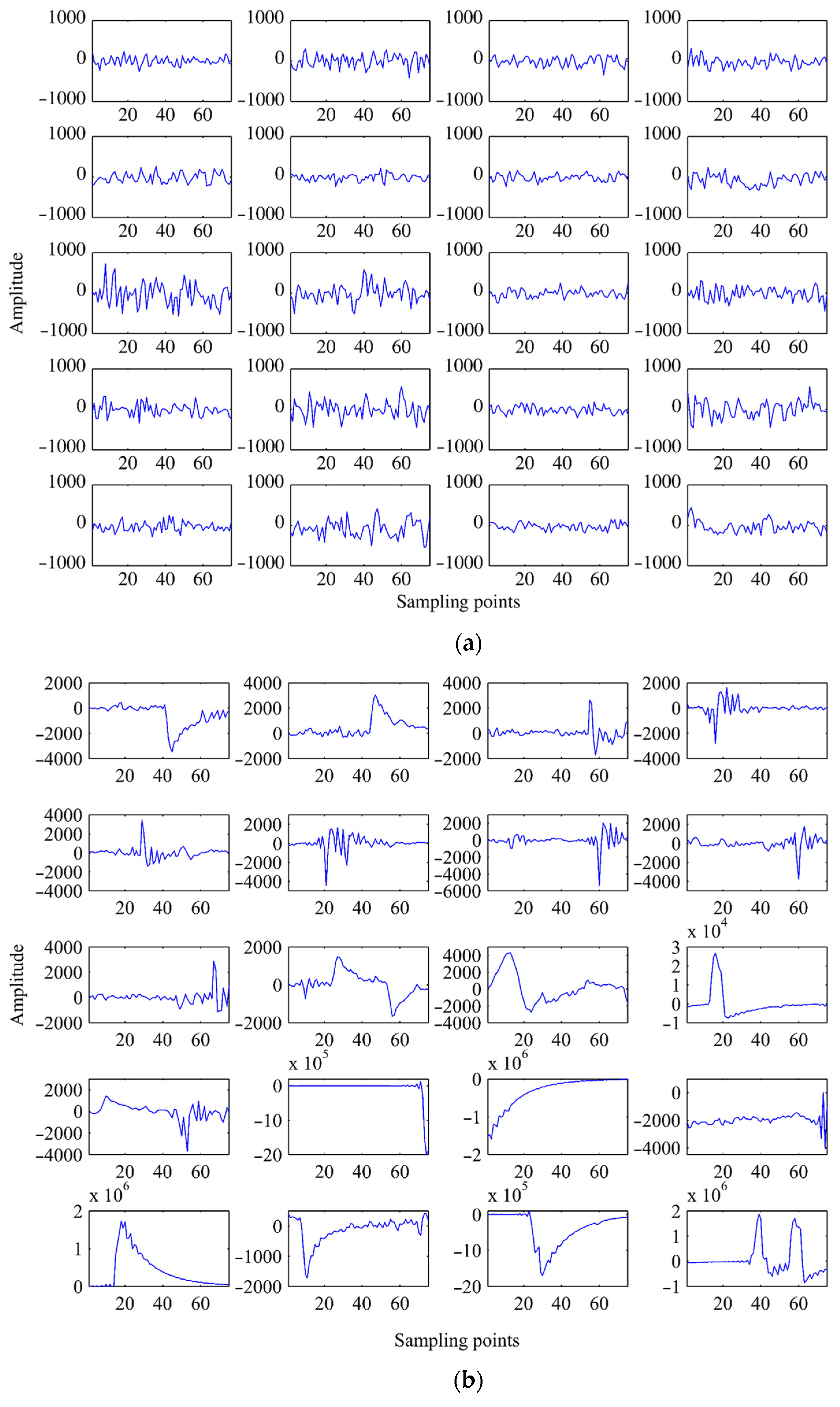
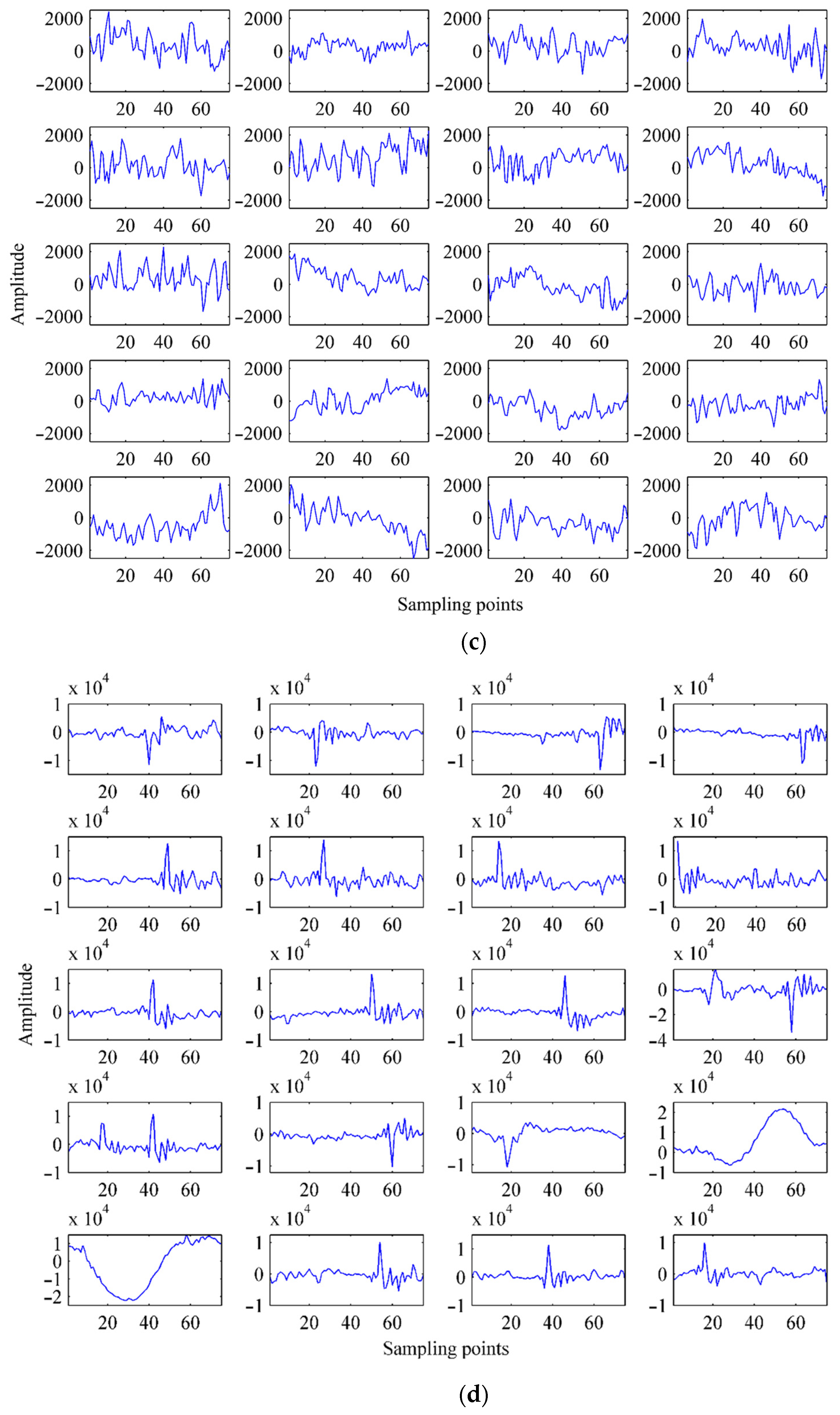
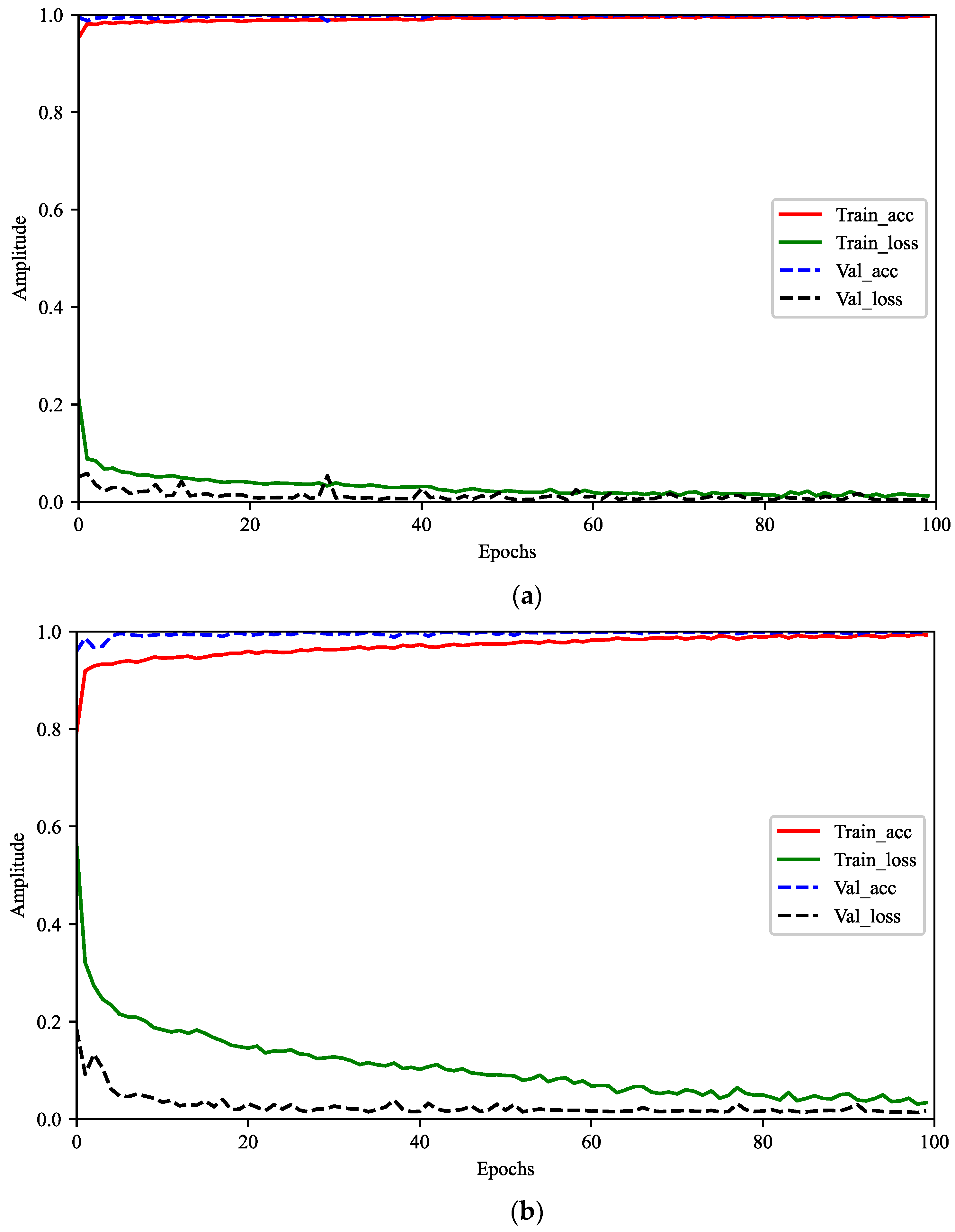
3.1. Sample Labeling and Model Training
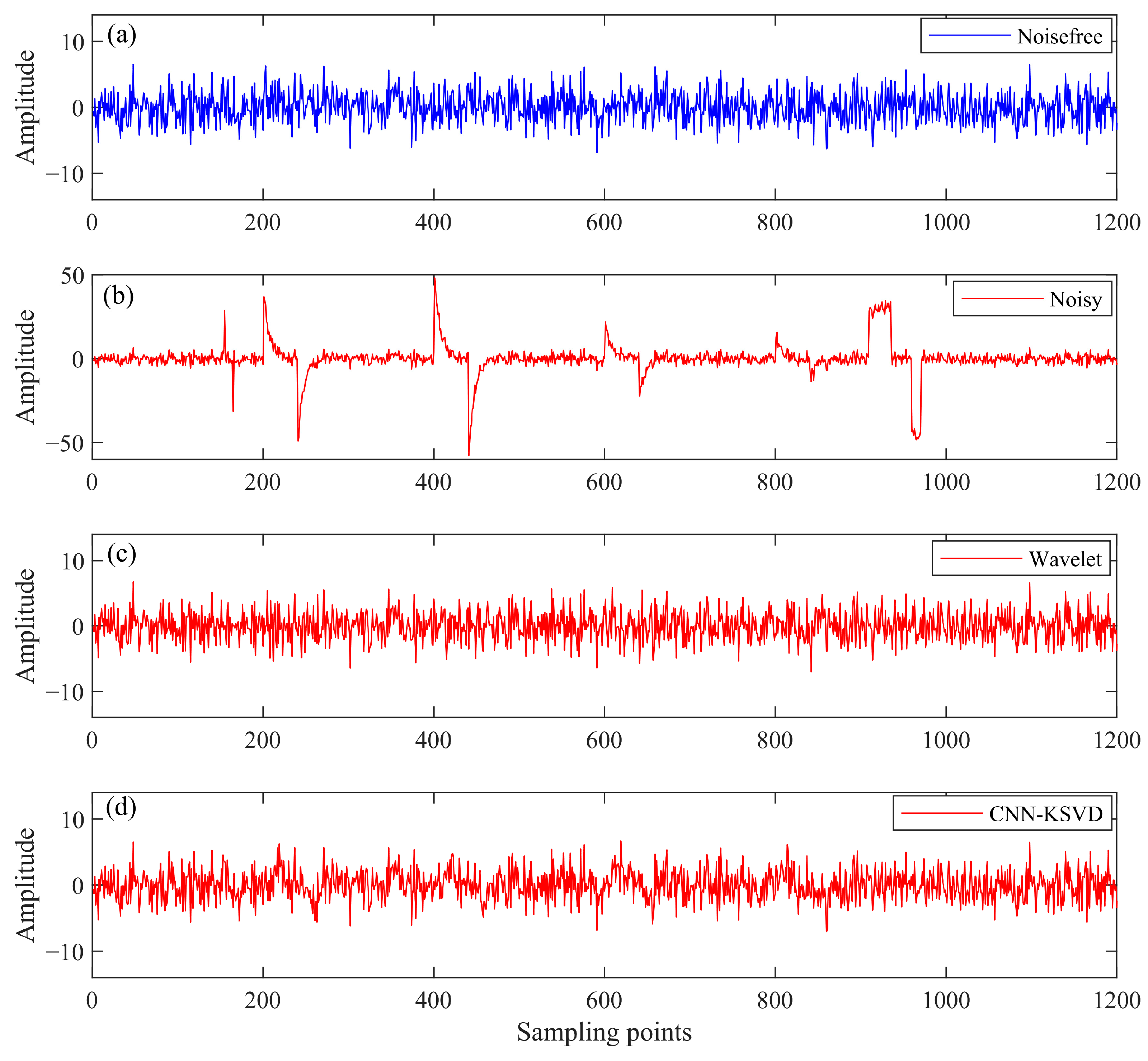
Samples are datasets for model training. Good training results mainly depend not on how good the model is, but more on the quantity and quality of the samples used for training. Zhang et al. [29] found that the recognition accuracy of MT data is positively correlated with the length of samples, but the training time will rise significantly with the increase in the sample length. The study also shows that when the sample length is 64 sampling points, very high classification accuracy can be obtained with high efficiency. The acquisition of MT data is sometimes discontinuous. Therefore, we set the sample length to 75 sampling points, a value close to 64, in order to not destroy the timing information of the original signal and to obtain high classification accuracy and efficiency. The observation duration of one sample is 0.5 s at a sampling rate of 150 Hz. Figure 5 shows some typical samples in the training set. It is found that the high-quality sample has a slow change in signal amplitude over time and a small average amplitude. Noisy samples often have shock-like structures with strong instantaneous energy. The average amplitude is significantly larger than the high-quality signal. Its magnitude is sometimes even several orders larger than the high-quality signals. It is well known that high-quality and noise-sample libraries have obvious differences, which are easily manually labeled or learned by the machine.
The training set of this paper is obtained from the measured data of the Lujiang–Zongyang ore concentration area. We make the training set of the electric channel data and the magnetic channel data separately due to the obvious difference between them. The number of electric channel samples is 14,000, including 7000 high-quality and 7000 noise samples. The number of magnetic track samples is 11,128, which includes 5564 high-quality and 5564 noise samples, respectively. A total of 6000 high-quality and 6000 noisy samples were selected from the electric channel sample library as training sets. The remaining high-quality data and noisy data were used as the validation set. The magnetic channel training set contains 5000 high-quality samples and 5000 noisy samples. The remaining samples were also reserved for the validation set.
The resulting sample library data were imported into the model for training. We adjusted the model or the sample library according to the training results. The training results of the electric channel data are shown in Figure 6a, including a training accuracy of 99.4%, a training loss of 0.016, and validation accuracy of 99.8%, and a validation loss of 0.015. The training results for the magnetic channel data are shown in Figure 6b. The training accuracy was 99.72%, and the training loss was 0.019. The validation set accuracy was 99.4%, and the validation loss was 0.014.

3.2. Simulation

We added some square-wave noise, spikes, and charge—discharge-like noise to the simulated noise-free MT signal and then processed the noise-added signal with the proposed method for a quantitative evaluation of the effectiveness. Figure 7a shows the result of the trained model’s identification of the simulated noisy MT data. Figure 7b shows the distribution of the MSE for each sample. Obviously, the high-quality signals are all accurately identified, and the MSE of the high-quality signals is smaller than the noise-containing signal. The largest MSE in the high-quality signal is the eighth sample, with an MSE of 2.46. Therefore, in the subsequent dictionary learning, the MSE less than or equal to 2.46 will be used as the iteration stop condition.
We took an MSE less than or equal to 2.46 as the constraint condition of K-SVD sparse decomposition and then denoised the noisy signal automatically. We compared this signal with the original noise-free signal and the signal obtained by Wavelet threshold denoising (hereinafter referred to as Wavelet). As shown in Figure 8, both Wavelet and the method proposed in this paper could remove most of the artificially added noise. However, the Wavelet method obviously removed some low-frequency signals because the denoised signal became more stationary. It can be seen from Table 1 that the effect of our new method is obvious and all-round superior to the Wavelet threshold denoising. The signal-to-noise ratio (SNR) improved from −11.6127 dB to 8.2648 dB. The increase is more than 19.87 dB. The MSE decreased from 8.6797 to 0.8803, the normalized cross-correlation (NCC) [22] increased from 0.2366 to 0.9251, and the reconstruction error (RE) decreased from 3.8075 to 0.3862. The simulation results also show that our method is suitable for the suppression of different types of noise.
Other main parameters of K-SVD in the experiment are set as follows. The number of atoms is 400, and the sparsity is set to 12. The influence of these parameters on the results is much smaller than the constraint condition of MSE. The Wavelet threshold denoising is performed at level 5 with db1. We used a hard threshold because it produced better SNR than soft thresholds in the experiment. The threshold selection rule is ‘minimaxi’, and single estimation rescaling is selected. All parameters were the best after many attempts.

4. Case Analysis

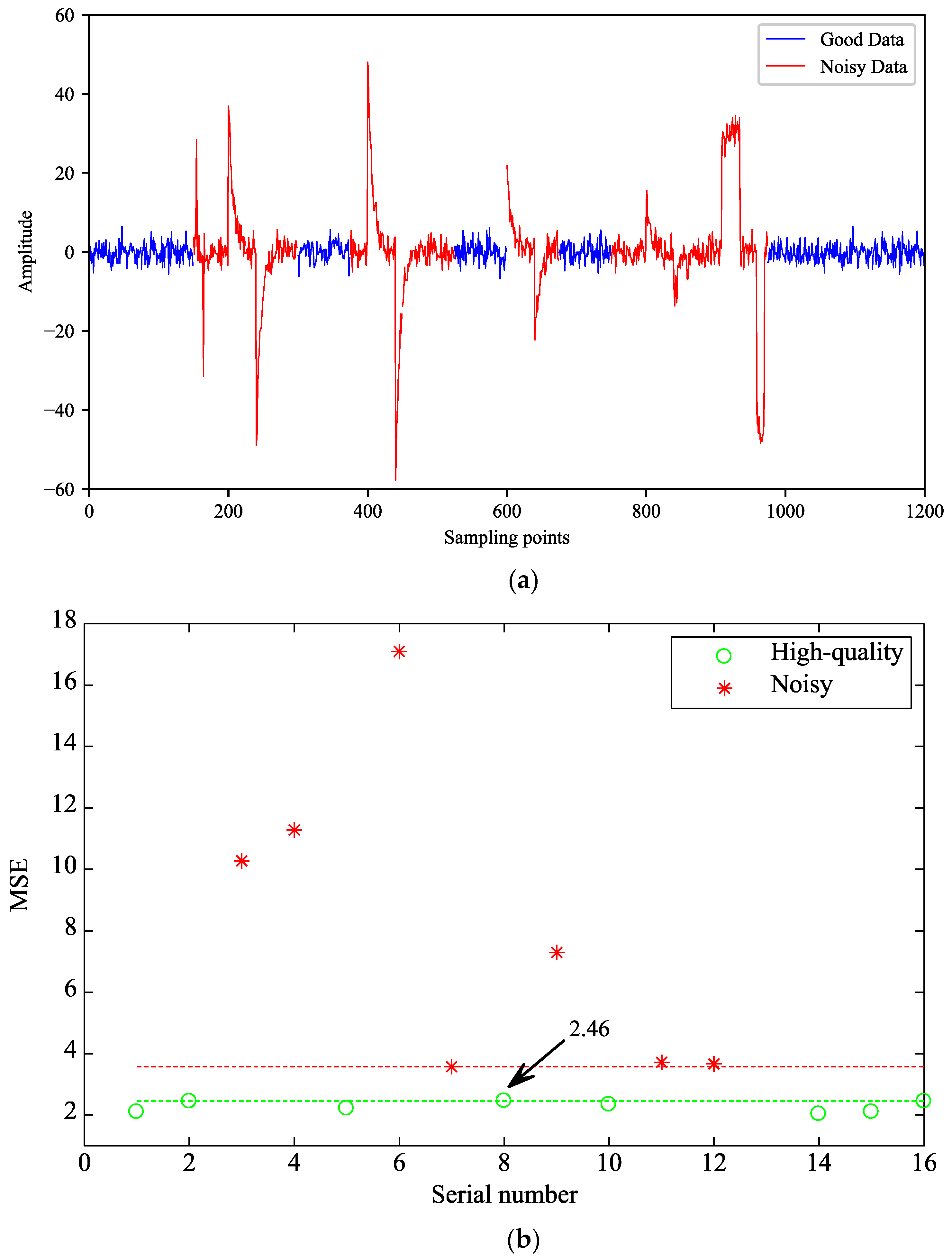
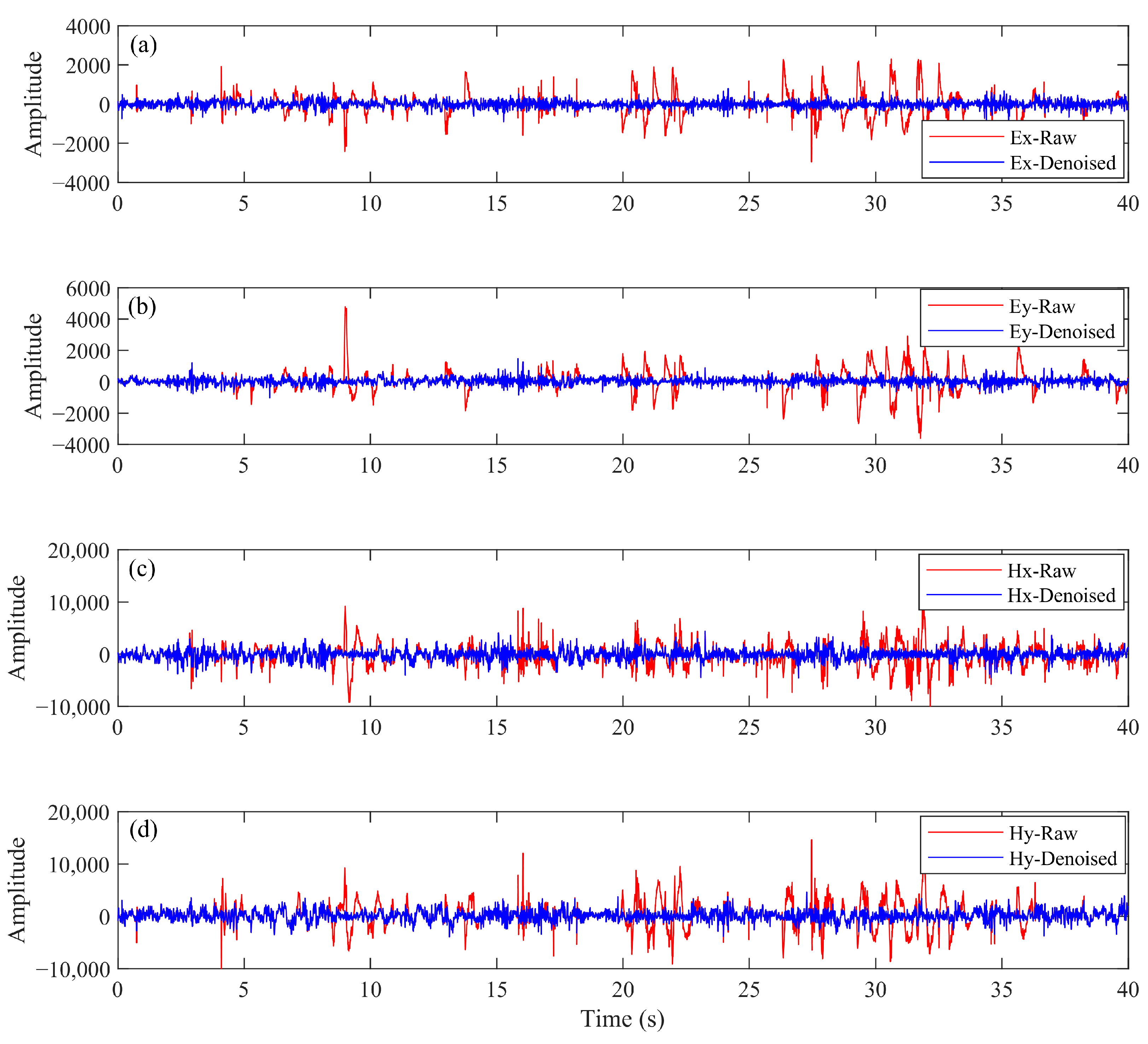
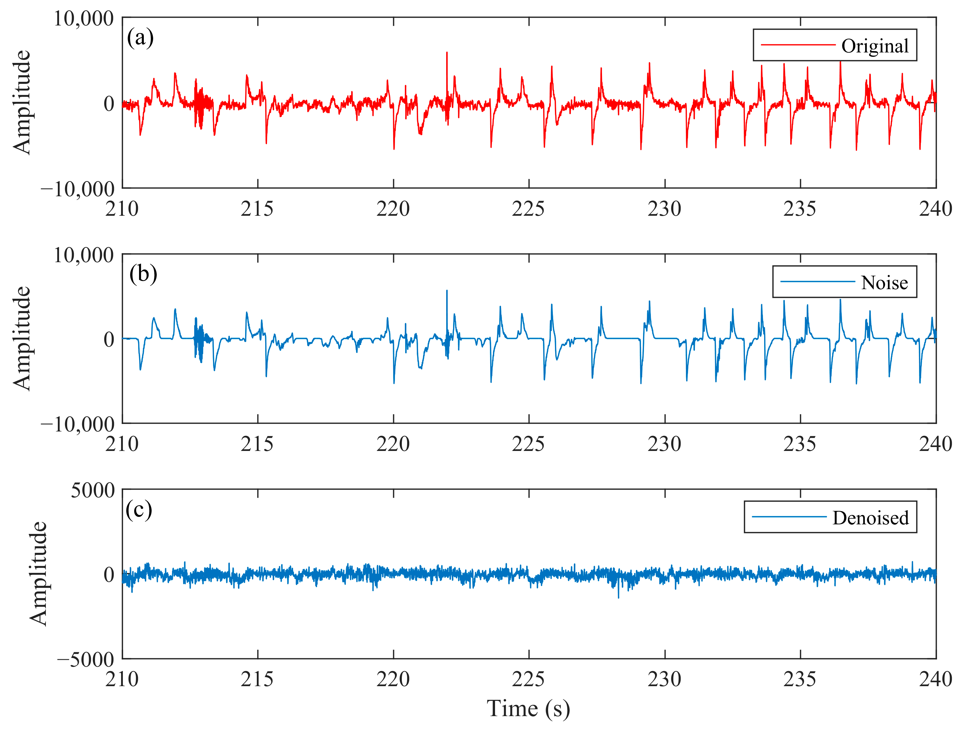
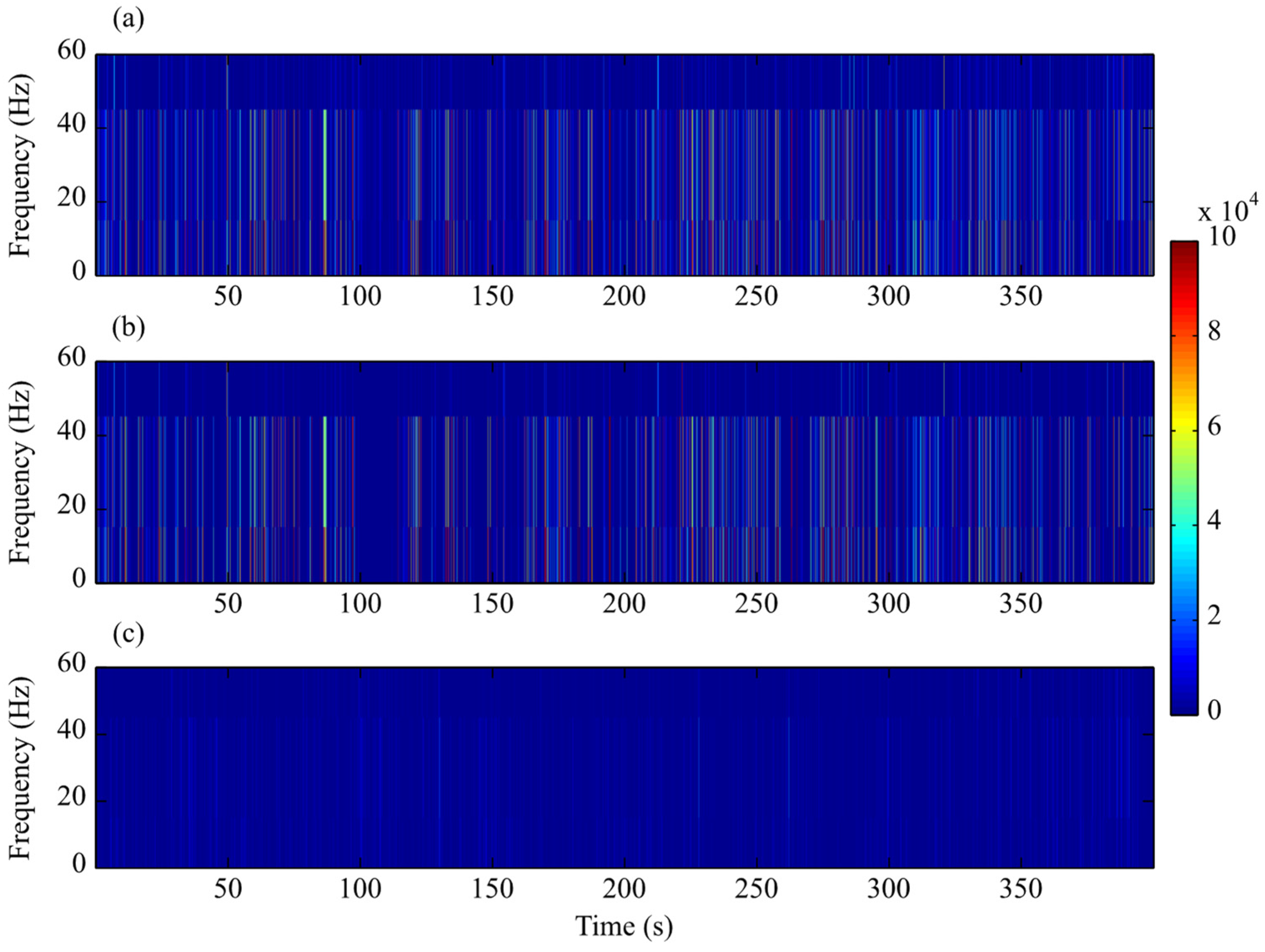
4.1. Time-Series Analysis

To verify the effectiveness of the proposed method in actual magnetotelluric data processing, we applied the proposed method to the time-series with strong interference collected in the ore-concentration areas of Lujiang–Zongyang. Figure 9 shows the recognition results of the Ex component of the real site BL14173A. It can be seen that the dataset was polluted by very strong and persistent cultural noise. In addition, a few spikes were marked in blue, which are noisy segments not accurately identified by the model. Since there are few instances of unrecognized noise and they are small in amplitude, the noise has little impact on the results. Figure 10 presents a partial segment of the results shown in Figure 9. Obviously, all large-amplitude cultural noises have been accurately identified. Compared with the results of manual marking, it was found that the recognition accuracy was as high as 95.66%.
As shown in Figure 11, the regular impulse waveform structure in the original signal is obviously not an effective magnetotelluric signal, because it is inconsistent with the characteristics of the magnetotelluric time-series that change slowly with time [7,11]. Therefore, it can be determined that the data of the four components collected in the site BL14182A are strongly and continuously polluted by the cultural noise. After using the method proposed in this paper, the noise of the large amplitude was accurately removed, and the high-quality fragment was not damaged. The amplitude and characteristics of the denoised fragments were very similar to those of high-quality fragments, indicating that the proposed method has high reliability.
We used the short-time Fourier transform to obtain the time-frequency spectrum of the signal shown in Figure 11. As shown in Figure 12, the time-frequency spectrum of the raw signal is very energetic below 40 Hz in some locations, which is inconsistent with the characteristics of the random distribution of natural MT signal energy. In other words, the noise is very strong and in the same frequency band as the effective signal. The denoised signal had no energy concentration period, which is closer to the characteristics of high-quality magnetotelluric signals. The time-frequency spectrum before and after denoising shows that our method completely removed the cultural noise in the same frequency band as the effective signal.
As shown in Figure 13, the original signal was polluted by continuous and strong charge–discharge-like noise, the noise profile extracted by the method proposed in this paper was smooth, and the amplitude corresponding to the time position of the high-quality fragment was 0, indicating that the proposed method removed the noise while not losing the effective signal in the high-quality fragment. The signal after denoising did not have a regular signal, and the amplitude changed slowly with time, which is in line with the characteristics of a pure magnetotelluric time-series. This example shows that the method proposed in this paper accurately identifies and effectively removes large-amplitude cultural noise, and deep learning effectively replaces the manual operation and automatically obtains the appropriate threshold.
Similarly, we analyzed the time-frequency spectrum of the denoised results. As shown in Figure 14, the noise of the original signal was mainly concentrated in the part below 40 Hz, and it can be seen that the effect of this noise on the resistivity and phase curve was also mainly concentrated in the part below 40 Hz. The time-frequency spectrum energy of the extracted noise signal is concentrated in the noisy period, and the energy is weak in the rest of the time period. After denoising, there is no period of abnormal-large energy in the signal, which shows that the proposed method accurately eliminates the noise.
It is worth noting that the observation time of the measured MT dataset used in this paper is about 70 min, and the length of the data of one channel is about 63,0000 sampling points. It takes about 192 s for CNN to train in an ordinary laptop (CPU, Intel i7-11800H; RAM, 16 GB; GPU, not called), but it only takes 8 s to call the trained model to complete the recognition of a channel’s data. The subsequent K-SVD denoising also takes only 2 s. Therefore, our method is efficient enough to deal with the massive MT data.

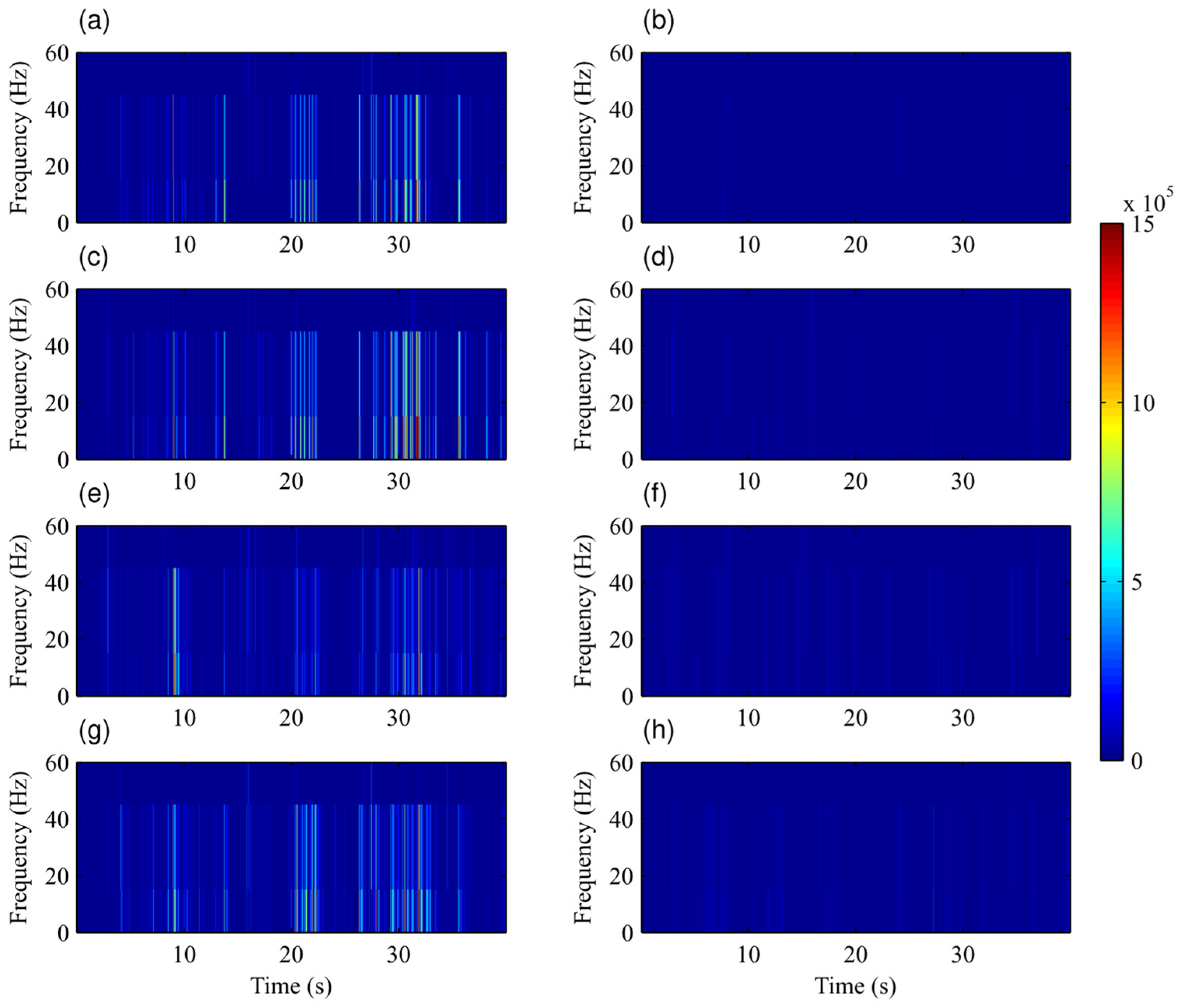
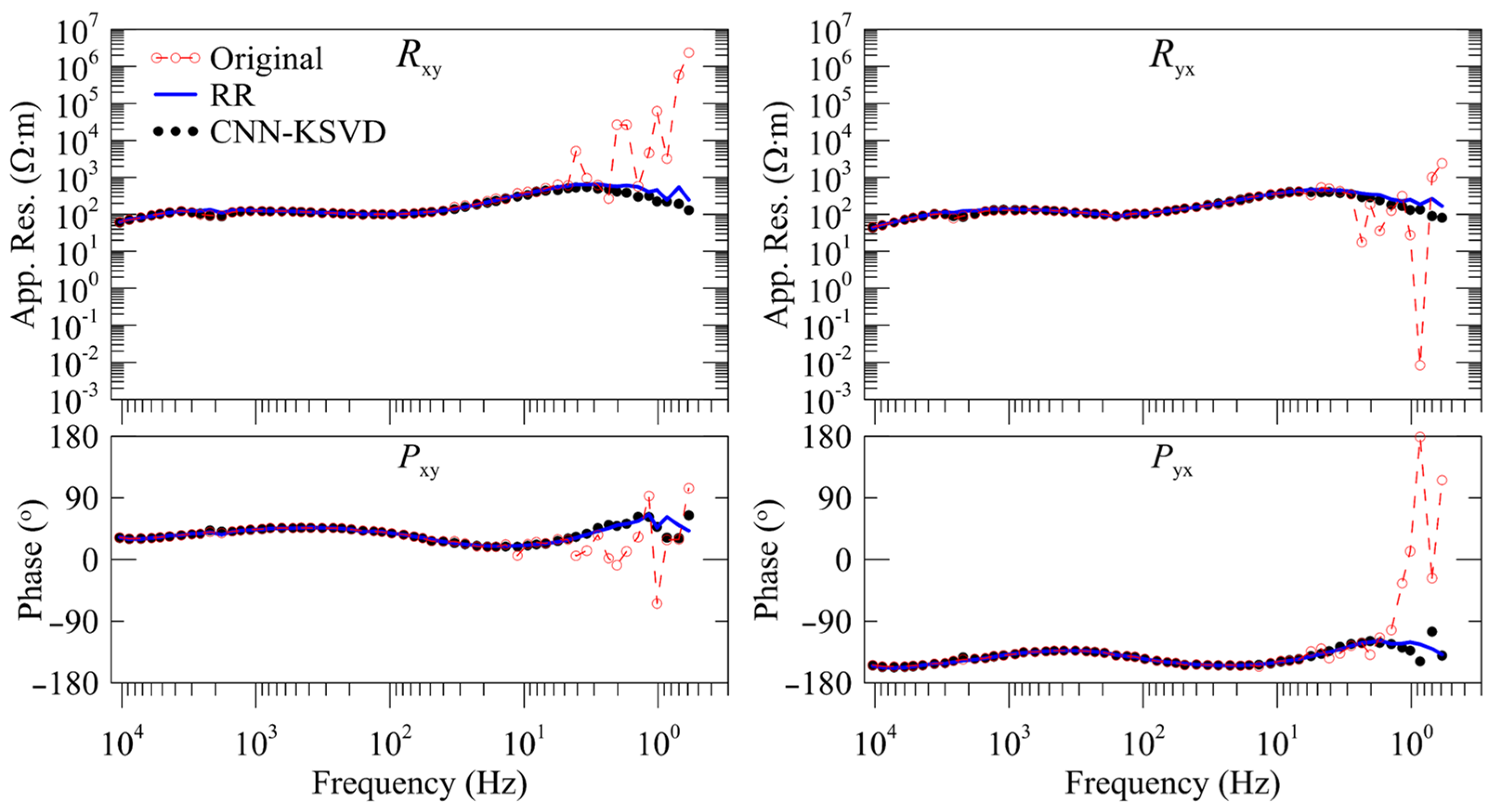
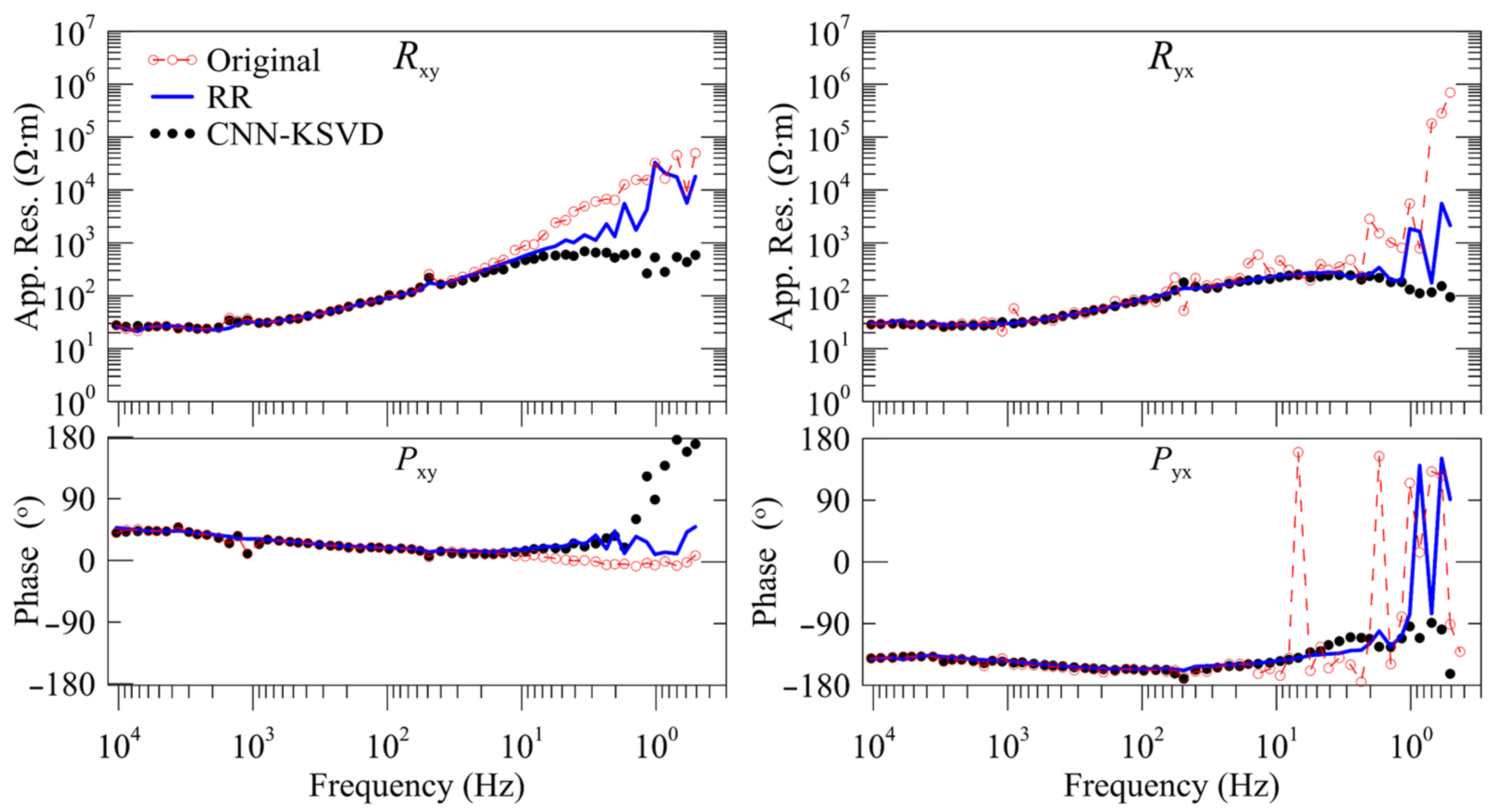
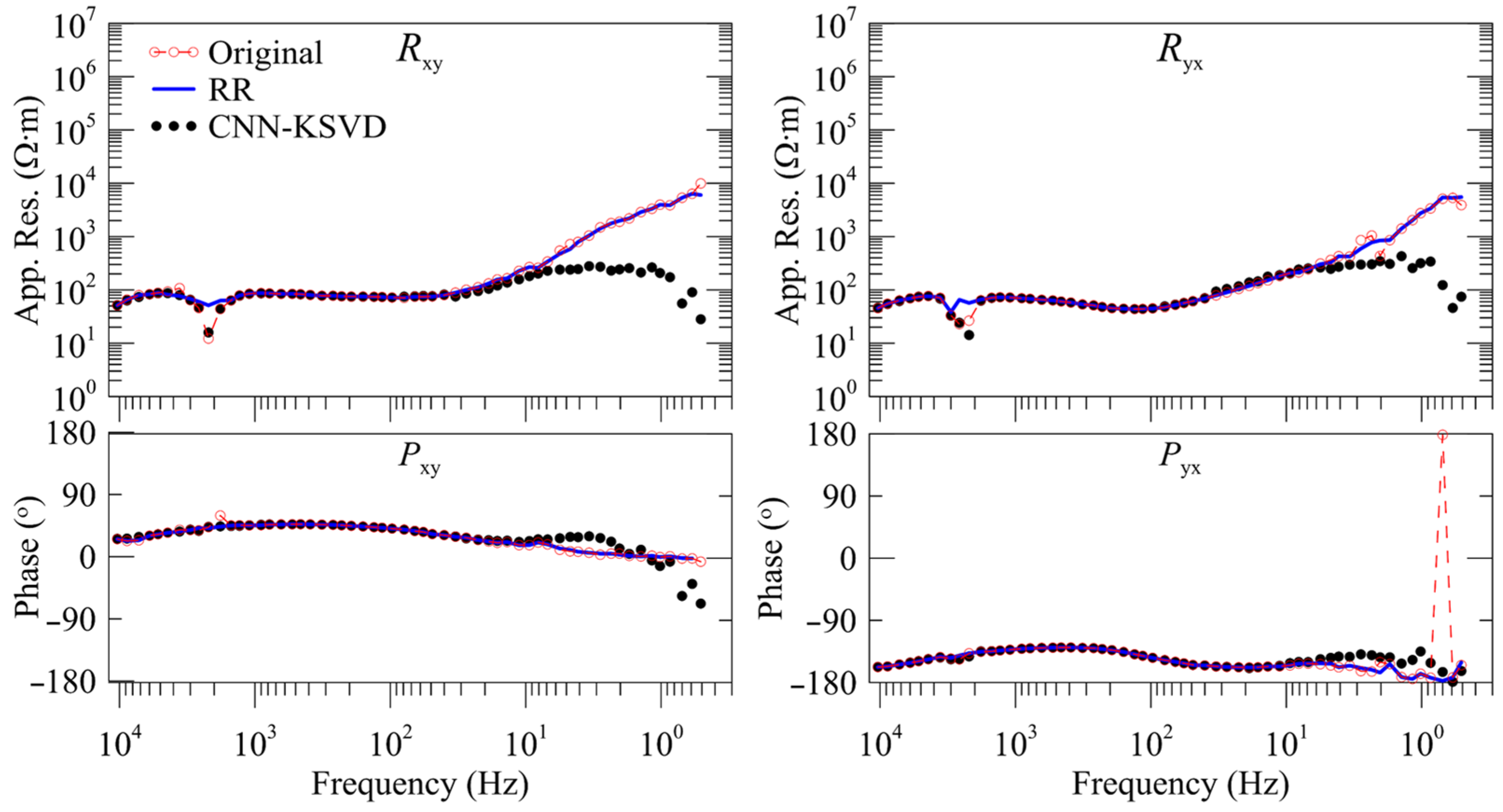
4.2. MT Response Analysis

In order to verify the reliability of the method, we calculated the magnetotelluric response from the processed data and compared it with the results of the remote reference method. The remote reference station is located on a sparsely populated hill in Zongyang County, Tongling City. It is about 45 km away from the local observation station. There is no obvious ambient noise near the remote reference station, and the apparent resistivity and phase curves are smooth. We selected three typical measured sites, BL14173A, BL14180A, and BL14182A, to display the sounding curves.
Figure 15 shows the apparent resistivity and phase curves calculated from the data collected at the station BL14180A in Lujiang–Zongyang ore concentration area in 2013. The recording time lasts about 70 min, and the data were polluted by strong cultural noise. The MT response calculated from the original data has a sharp jump and a serious distortion in the part below 10 Hz. The convergence error of such a curve is too large to fit during the inversion. The curves obtained by our method are obviously improved. Except for the part below 1 Hz, the other curves are continuous and smooth. The results obtained by our method almost coincide with those obtained by the remote reference method except for the part below 1 Hz. This shows that the result of my method is reliable.
Figure 16 shows the MT response curves of the station BL14173A. The original response curves have obvious distortion below the 1000 Hz in the YX direction, and there are many outliers. Obviously, the sounding curves in this direction are of poor quality. After the processing of the remote reference method, the curves were significantly improved. Except for the visible distortion at 1 Hz and below, the curves of other parts were relatively smooth. The results obtained by our method are generally consistent with the remote reference processing in the part greater than 1 Hz, but the continuity of the curves around 1 Hz and below are better than that achieved with the remote reference method.
In the XY direction, the original sounding curves are relatively smooth and are easy to be mistaken for high-quality curves. However, this is a typical feature caused by serious near-source noise [38], because its apparent resistivity curve shows a 45° asymptote rise in the part below 40 Hz, and the phases are almost all 0. The conclusion can also be proved by the time-frequency spectrum shown in Figure 14, because there is intensive noise between 0 and 40 Hz. After the processing of the remote reference method, the near-source effect from 5 Hz to 40 Hz is significantly improved, the curves are smooth, and the phases are no longer 0. However, the part below 5 Hz still has an obvious upward trend of 45°, and some phases are still very close to 0. After processing by our method, except for the visible distortion of the phase curve below 2 Hz, the result of the other parts is obviously better than that of the remote reference processing. The similarity between the XY direction curve and the YX direction curve is high, which also indicates the reliability of the results to a certain extent.
As shown in Figure 17, the apparent resistivity curves at the station BL14182A calculated using the original data show a 45° asymptote rise in the part below 40 Hz, and the corresponding phase curves slowly approach 0 or −180°, which is obviously caused by serious near-source interference. In addition, the dead-band curves near 2000 Hz also have obvious distortion. After the remote reference processing, the dead-band curves near 2000 Hz were significantly improved, but the near-source effect was not improved. Nevertheless, after processing by our new method, the near-source effect of the curves below 40 Hz are greatly improved, the sounding curves above 1 Hz are generally smooth, and most of the phase values return to the normal range. Although we cannot confirm that the results obtained by our method are accurate, we can be sure that our results are more reasonable than the results of the original sounding curves and the curves obtained by the remote reference method.

5. Conclusions

The existing sparse decomposition denoising methods need to manually set the iteration stop condition, which not only has a large workload and time consumption but also is prone to subjective bias. More importantly, these methods cannot realize batch data processing because each dataset has different characteristics. Therefore, this paper uses the deep convolution neural network to autonomously learn the features of high-quality magnetotelluric data from the observed time-series and takes them as the constraints of subsequent dictionary learning to realize the adaptive sparse decomposition. Based on this, we propose a new, adaptive magnetotelluric noise cancellation method called CNN-KSVD.
The effectiveness and reliability of the proposed method were verified by the analysis of simulation data and measured data. This method was found to be able to greatly increase the signal-to-noise ratio of magnetotelluric data and improve the estimation of apparent resistivity and phase. The examples also show that our method can achieve the comparable effect as the outcomes of processing with a good remote reference. When there is no remote reference station or the remote reference processing is not effective, our method can be used as an effective alternative.
The method does not need manual intervention and uses completely unified parameters and standardized processing for all data so that the method enables batch processing of sparse decomposition denoising for magnetotelluric data to be possible, which is hard to realize using the existing sparse decomposition denoising method. Furthermore, the fully automated processing completely eliminates subjective bias.
Sparse decomposition often has the disadvantage of low efficiency, but the K-SVD dictionary learning method used in this paper only takes a few seconds to process an AMT data set with an observation time of about 70 min. CNN needs hundreds of seconds or even thousands of seconds to train the model, but in actual processing, it only needs to call the trained model to learn the parameters, and this process will not exceed a few seconds. Therefore, this method has high efficiency and brings great convenience to mass magnetotelluric data processing.
Sparse decomposition methods, including K-SVD, are suitable for removing noise with certain morphological differences from the signal, so our method may not be competent to eliminate Gaussian white noise from MT data. In most cases, the MT response curves obtained by our method are not very smooth below 1 Hz, which shows that the denoising accuracy of the method has room for improvement. The recognition effect of our method is also not perfect, which is mainly related to the quantity and quality of training samples, and the accuracy of dictionary learning. In addition, there is a certain relationship with the network structure. The denoising effect of the method is expected to be improved by further expanding the number of samples and optimizing the network structure. This is the focus of our follow-up study.

Author Contributions

G.L.: Conceptualization, Methodology, Software, Visualization, Investigation, Supervision, Funding Acquisition, Formal Analysis, Writing—Original Draft; X.G.: Software, Validation, Writing—Review and Editing; Z.R.: Funding Acquisition, Resources, Supervision, Conceptualization, Data Curation, Writing—Review and Editing; Q.W.: Supervision, Funding Acquisition, Formal Analysis; X.L.: Methodology, Software, Data Curation; L.Z.: Methodology, Validation, Writing—Review and Editing; D.X.: Data Curation; C.Z.: Review and Editing. All authors have read and agreed to the published version of the manuscript.

Funding

This research is funded by the National Natural Science Foundation of China (41904076 and 41904072), the Shenzhen Science and Technology Program (JCYJ20210324125601005), the Innovation-Driven Project of Central South University (2021zzts0257), the Open Fund from Key Laboratory of Metallogenic Prediction of Nonferrous Metals and Geological Environment Monitoring, Ministry of Education (2021YSJS02), the Regional Innovation Cooperation Programs of Sichuan province (2021YFQ0050), the Natural Science Foundation of Jiangxi Province (20192BAB212009 and 20202BABL211017), and the National Key R&D Program of China (2018YFC0603202).

Data Availability Statement

Data associated with this research are available and can be obtained by contacting the corresponding author.

Conflicts of Interest

The authors declare no conflict of interest.

References

  1. Tikhonov, A.N. On determining electrical characteristics of the deep layers of the Earth’s crus. Dokl. Akad. Nauk 1950, 73, 295–297. [Google Scholar]
  2. Cagniard, L. Basic theory of the magnetotelluric method of geophysical prospecting. Geophysics 1953, 18, 605–635. [Google Scholar] [CrossRef]
  3. Yu, N.; Unsworth, M.; Wang, X.; Li, D.; Wang, E.; Li, R.; Hu, Y.; Cai, X. New insights into crustal and mantle flow beneath the Red River Fault zone and adjacent areas on the southern margin of the Tibetan Plateau revealed by a 3D magnetotelluric study. J. Geophys. Res. Solid Earth 2020, 125, e2020JB019396. [Google Scholar] [CrossRef]
  4. Li, R.H.; Yu, N.; Wang, X.B.; Liu, Y.; Cai, Z.K.; Wang, E.C. Model-Based Synthetic Geoelectric Sampling for Magnetotelluric Inversion With Deep Neural Networks. IEEE Trans. Geosci. Remote Sens. 2022, 60, 4500514. [Google Scholar] [CrossRef]
  5. Xu, Y.X.; Zhang, Y.; Yang, B.; Bao, X.W. Phanerozoic evolution of lithospheric structures of the North China Craton. Geophys. Res. Lett. 2022, 49, e2022GL098341. [Google Scholar] [CrossRef]
  6. Simpson, F.; Bahr, K. Practical Magnetotellurics; Cambridge University Press: Cambridge, UK, 2005. [Google Scholar]
  7. Jiang, F.; Chen, X.B.; Unsworth, M.J.; Cai, J.T.; Han, B.; Wang, L.F.; Dong, Z.Y.; Cui, T.F.; Zhan, Y.; Zhao, G.Z.; et al. Mechanism for the uplift of Gongga Shan in the southeastern Tibetan Plateau constrained by 3D magnetotelluric data. Geophys. Res. Lett. 2022, 49, e2021GL097394. [Google Scholar] [CrossRef]
  8. Giuseppe, M.G.D.; Troiano, A.; Patella, D. Separation of plain wave and near field contributions in Magnetotelluric time series: A useful criterion emerged during the Campi Flegrei (Italy) prospecting. J. Appl. Geophys. 2018, 156, 55–66. [Google Scholar] [CrossRef]
  9. Gamble, T.D.; Goubau, W.M.; Clarke, J. Magnetotellurics with a remote magnetic reference. Geophysics 1979, 44, 53–68. [Google Scholar] [CrossRef]
  10. Egbert, G.D.; Booker, J.R. Robust estimation of geomagnetic transfer functions. Geophys. J. Inter. 1986, 87, 173–194. [Google Scholar] [CrossRef]
  11. Egbert, G.D. Robust multiple-station magnetotelluric data processing. Geophys. J. Int. 1997, 130, 475–496. [Google Scholar] [CrossRef]
  12. Trad, D.O.; Travassos, J.M. Wavelet filtering of magnetotelluric data. Geophysics 2000, 65, 482–491. [Google Scholar] [CrossRef]
  13. Neukirch, M.; Garcia, X. Nonstationary magnetotelluric data processing with instantaneous parameter. J. Geophys. Res. Solid Earth 2014, 199, 1634–1654. [Google Scholar] [CrossRef]
  14. Li, G.; Liu, X.; Tang, J.; Deng, J.; Hu, S.; Zhou, C.; Chen, C.; Tang, W. Improved shift-invariant sparse coding for noise attenuation of magnetotelluric data. Earth Planets Space 2020, 72, 15. [Google Scholar] [CrossRef]
  15. Li, G.; Liu, X.; Tang, J.; Li, J.; Ren, Z.; Chen, C. De-noising low-frequency magnetotelluric data using mathematical morphology filtering and sparse representation. J. Appl. Geophys. 2020, 172, 103919. [Google Scholar] [CrossRef]
  16. Li, J.; Liu, X.Q.; Li, G.; Tang, J.T. Magnetotelluric Noise Suppression Based on Impulsive Atoms and NPSO-OMP Algorithm. Pure Appl. Geophys. 2020, 177, 5275–5297. [Google Scholar] [CrossRef]
  17. Zhou, R.; Han, J.T.; Guo, Z.Y.; Li, T.L. De-Noising of Magnetotelluric Signals by Discrete Wavelet Transform and SVD Decomposition. Remote Sens. 2021, 13, 4932. [Google Scholar] [CrossRef]
  18. Cai, J.H. A combinatorial filtering method for magnetotelluric data series with strong interference. Arab. J. Geosci. 2016, 9, 628. [Google Scholar]
  19. Li, G.; Xiao, X.; Tang, J.T.; Li, J.; Zhu, H.J.; Zhou, C.; Yan, F.B. Near-source noise suppression of AMT by compressive sensing and mathematical morphology filtering. Appl. Geophys. 2017, 14, 581–589. [Google Scholar] [CrossRef]
  20. Li, J.; Peng, Y.Q.; Tang, J.T.; Li, Y. Denoising of magnetotelluric data using K-SVD dictionary training. Geophys. Prospect. 2021, 69, 448–473. [Google Scholar] [CrossRef]
  21. Xue, S.Y.; Yin, C.C.; Su, Y.; Liu, Y.H.; Wang, Y.; Liu, C.H.; Xiong, B.; Sun, H.F. Airborne electromagnetic data denoising based on dictionary learning. Appl. Geophys. 2020, 17, 306–313. [Google Scholar] [CrossRef]
  22. Li, G.; He, Z.; Tang, J.T.; Deng, J.Z.; Liu, X.; Zhu, H.J. Dictionary learning and shift-invariant sparse coding denoising for controlled-source electromagnetic data combined with complementary ensemble empirical mode decomposition. Geophysics 2021, 86, E185–E198. [Google Scholar] [CrossRef]
  23. Zhang, P.; Pan, X.; Liu, J. Denoising Marine Controlled Source Electromagnetic Data Based on Dictionary Learning. Minerals 2022, 12, 682. [Google Scholar] [CrossRef]
  24. Jiang, Z.J.; Mallants, D.; Peeters, L.; Gao, L.; Mariethoz, G. High-resolution palaeovalley classification from airborne electromagnetic imaging and deep neural network training using digital elevation model data. Hydrol. Earth Syst. Sci. 2019, 23, 2561–2580. [Google Scholar] [CrossRef]
  25. Li, J.F.; Liu, Y.H.; Yin, C.C.; Ren, X.Y.; Su, Y. Fast imaging of time-domain airborne EM data using deep learning technology. Geophysics 2020, 85, E163–E170. [Google Scholar] [CrossRef]
  26. Moghadas, D. One-dimensional deep learning inversion of electromagnetic induction data using convolutional neural network. Geophys. J. Int. 2020, 222, 247–259. [Google Scholar] [CrossRef]
  27. Wu, X.; Xue, G.; He, Y.; Xue, J. Removal of the Multisource Noise in Airborne Electromagnetic Data Based on Deep Learning. Geophysics 2020, 85, B207–B222. [Google Scholar] [CrossRef]
  28. Wu, S.H.; Huang, Q.H.; Zhao, L. De-noising of transient electromagnetic data Based on the long short-term memory-autoencoder. Geophys. J. Int. 2021, 224, 669–681. [Google Scholar] [CrossRef]
  29. Zhang, L.; Ren, Z.Y.; Xiao, X.; Tang, J.T.; Li, G. Identification and Suppression of Magnetotelluric Noise via a Deep Residual Network. Minerals 2022, 12, 766. [Google Scholar] [CrossRef]
  30. Li, J.; Zhang, X.; Gong, J.; Tang, J.; Ren, Z.; Li, G.; Deng, Y.; Cai, J. Signal-noise identification of magnetotelluric signals using fractal-entropy and clustering algorithm for targeted de-noising. Fractals 2018, 26, 1840011. [Google Scholar] [CrossRef]
  31. Manoj, C.; Nagarajan, N. The application of artificial neural networks to magnetotelluric time-series analysis. Geophys. J. Int. 2003, 153, 409–423. [Google Scholar] [CrossRef]
  32. Fukushima, K. Neocognitron: A self-organizing neural network model for a mechanism of pattern recognition unaffected by shift in position. Biol. Cybern. 1980, 36, 193–202. [Google Scholar] [CrossRef] [PubMed]
  33. Schmidhuber, J. Deep learning in neural networks: An overview. Neural Netw. 2015, 61, 85–117. [Google Scholar] [CrossRef] [PubMed]
  34. LeCun, Y.; Kavukcuoglu, K.; Farabet, C. Convolutional networks and applications in vision. In Proceedings of the 2010 IEEE International Symposium on Circuits and Systems, Paris, France, 30 May–2 June 2010; pp. 253–256. [Google Scholar]
  35. Olshausen, B.A.; Field, D.J. Emergence of simple-cell receptive field properties by learning a sparse code for natural images. Nature 1996, 381, 607–609. [Google Scholar] [CrossRef] [PubMed]
  36. Engan, K.; Aase, S.O.; Husoy, J.H. Method of optimal directions for frame design. In Proceedings of the 1999 IEEE International Conference on Acoustics Speech, and Signal Processing, Phoenix, AZ, USA, 15–19 March 1999; pp. 2443–2446. [Google Scholar]
  37. Aharon, M.; Elad, M.; Bruckstein, A. K-SVD: An Algorithm for Designing Overcomplete Dictionaries for Sparse Representation. IEEE Trans. Signal Process. 2006, 54, 4311–4322. [Google Scholar] [CrossRef]
  38. Tang, J.T.; Zhou, C.; Wang, X.Y.; Xiao, X.; Lu, Q.T. Deep electrical structure and geological significance of Tongling ore district. Tectonophysics 2013, 606, 78–96. [Google Scholar] [CrossRef]
Figure 1. Manually marked real MT data. The red line indicates noisy clips, and the blue line indicates high-quality clips.
Minerals 12 01012 g001
Figure 2. Mean square error (MSE) distribution of randomly selected measured magnetotelluric (MT) data. The red stars represent strong-noise samples, and the green circles represent high-quality samples. The abscissa represents the serial number of the sample.
Minerals 12 01012 g002
Figure 3. The steps of the proposed method. (a) Raw signal. (b) Noisy signal. (c) High-quality signal. (d) Reconstructed signal.
Minerals 12 01012 g003
Figure 4. The structure of convolutional neural network (CNN). Conv1D represents the one-dimensional convolution layer; MaxPooling1D represents the one-dimensional maximum pooling layer.
Minerals 12 01012 g004
Figure 5. The typical samples in the training set. (a) High-quality electric channel samples. (b) Noisy magnetic channel samples. (c) High-quality magnetic channel samples. (d) Noisy magnetic channel signal samples.
Minerals 12 01012 g005aMinerals 12 01012 g005b
Figure 6. Results of the model training. (a) The training results of electric channel samples. (b) The training results of magnetic channel samples. The red and green solid lines represent training accuracy and training loss, respectively; the blue and black dotted lines represent validation accuracy and validation loss, respectively.
Minerals 12 01012 g006
Figure 7. (a) Identification results of the simulated signal. The red line indicates noisy clips, and the blue line indicates high-quality clips. (b) The MSE distribution of the simulation signals. The red stars represent noisy samples, and the green circles represent high-quality samples.
Minerals 12 01012 g007
Figure 8. Denoising effect of the simulated signal. (a) Noise-free signal. (b) Noisy signal. (c) Signal denoised by the Wavelet threshold method. (d) Signal denoised by the CNN-KSVD method.
Minerals 12 01012 g008
Figure 9. Recognition results of the Ex component of the real site BL14173A. The red line indicates noisy data, and the blue line indicates high-quality data.
Minerals 12 01012 g009
Figure 10. Partial display of identification results of the Ex component in the real site BL14173A. The red line indicates noisy data, and the blue line indicates high-quality data.
Minerals 12 01012 g010
Figure 11. Denoising results of real MT data collected in the station of BL14182A. (ad) represent the Ex, Ey, Hx, and Hy components, respectively. The red line represents the raw data and the blue line represents the high-quality data obtained by our new method.
Minerals 12 01012 g011
Figure 12. Time-frequency spectrum of the real data sets BL14182A before (the left) and after (the right) denoising. (ah) From top to bottom are the Ex, Ey, Hx, and Hy components, respectively.
Minerals 12 01012 g012
Figure 13. The denoising effect of a segment in the Ex component of the station BL14173. (a) Original signal. (b) Extracted noise. (c) Denoised signal.
Minerals 12 01012 g013
Figure 14. The time-frequency spectrum of the signals shown in Figure 13. (a) Raw time-frequency spectrum. (b) Time-frequency spectrum of the extracted noise. (c) Denoised time-frequency spectrum.
Minerals 12 01012 g014
Figure 15. The apparent resistivity and phase curves of real site BL14180A. Rxy and Ryx in the upper panels represent the apparent resistivity in the XY direction and YX direction, respectively; Pxy and Pyx in the bottom panels represent the phase in the XY direction and YX direction, respectively; the red hollow circle represents the curves calculated from the original noisy data (Original), the blue solid line represents the curves treated by the remote reference processing (RR), and the black solid circle represents the curves calculated using the data denoised by our method.
Minerals 12 01012 g015
Figure 16. The apparent resistivity and phase curves of real site BL14173A. Rxy and Ryx in the upper panels represent the apparent resistivity in XY direction and YX direction, respectively; Pxy and Pyx in the bottom panels represent the phase in XY direction and YX direction, respectively; the red hollow circle represents the curves calculated from the original noisy data (Original), the blue solid line represents the curves treated by the remote reference processing (RR), and the black solid circle represents the curves calculated using the data denoised by our method.
Minerals 12 01012 g016
Figure 17. The apparent resistivity and phase curves of the real site BL14182A. Rxy and Ryx in the upper panels represent the apparent resistivity in XY direction and the YX direction, respectively; Pxy and Pyx in the bottom panels represent the phase in the XY direction and the YX direction, respectively; the red hollow circle represents the curves calculated from the original noisy data (Original), the blue solid line represents the curves treated by the remote reference processing (RR), and the black solid circle represents the curves calculated using the data denoised by our method.
Minerals 12 01012 g017
Table 1. Statistics of denoising results with different methods.
MethodsSNRMSENCCRE
Noisy−11.61278.67970.23663.8075
Wavelet5.90441.15520.86730.5067
CNN-KSVD8.26480.88030.92510.3862
Publisher’s Note: MDPI stays neutral with regard to jurisdictional claims in published maps and institutional affiliations.

