
Protected Areas vs. Highway Construction—Problem of Environmental Pollution


Abstract
:1. Introduction
2. Materials and Methods
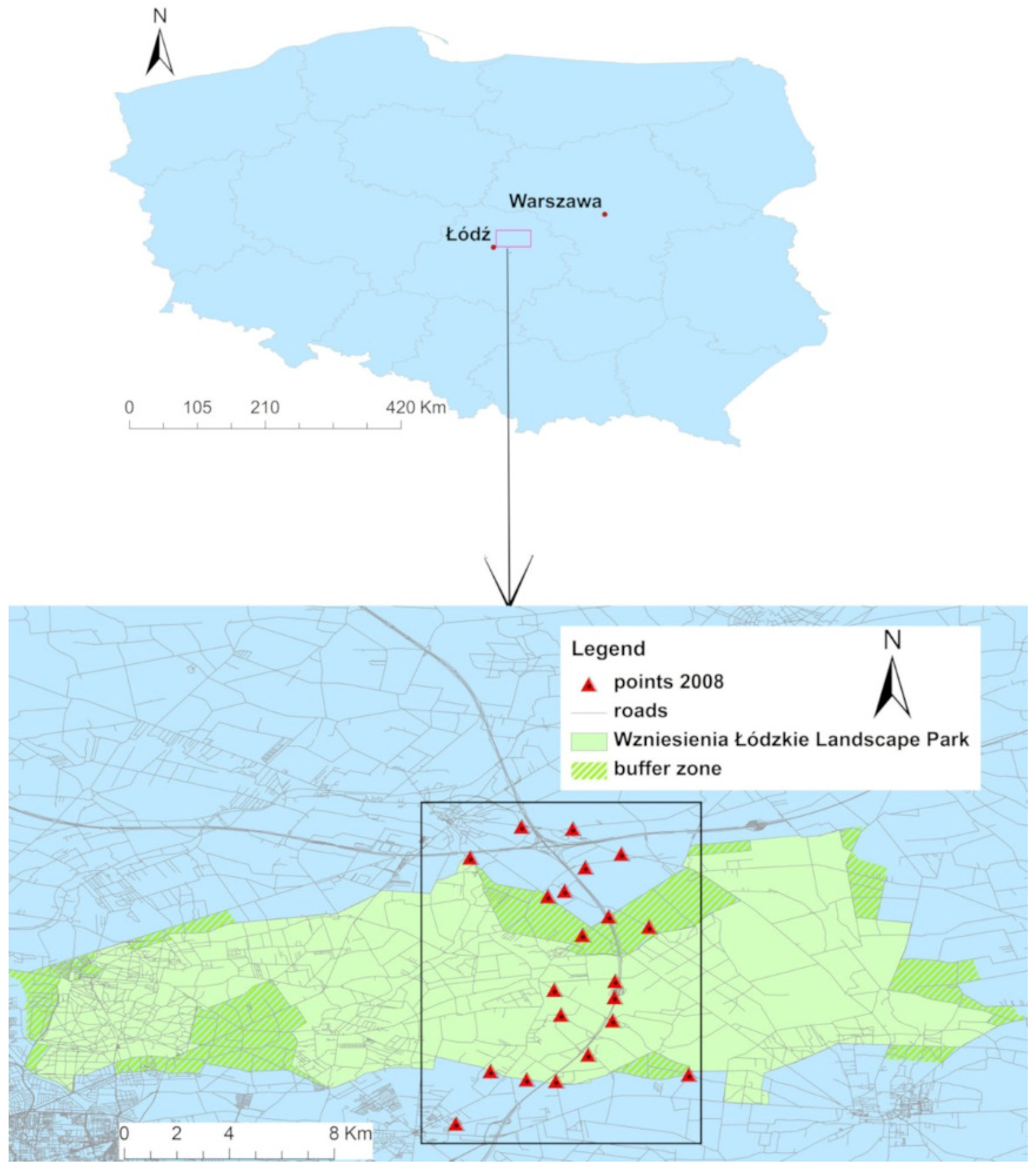
2.1. Study Area
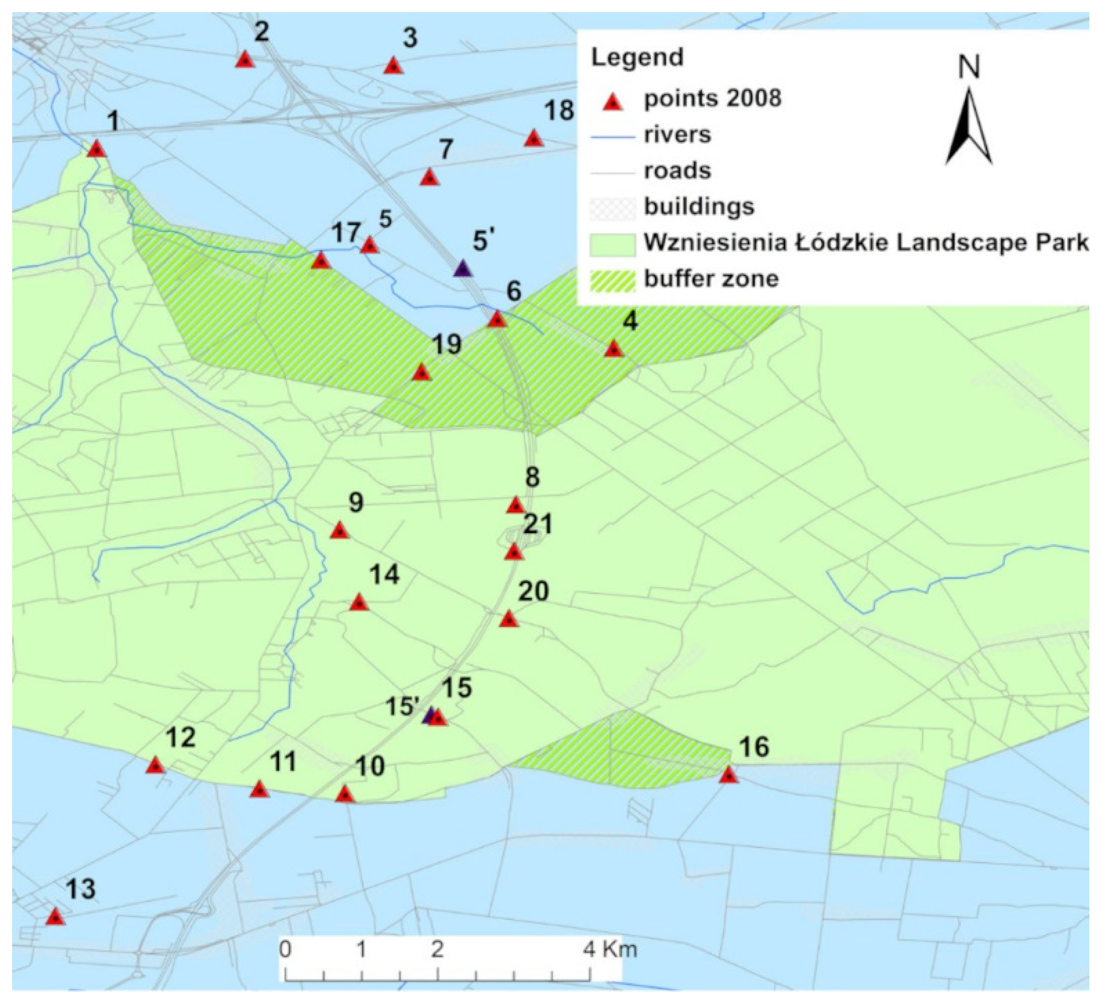
2.2. Soil Sampling
2.3. Soil Characterization—Analytical and Statistical Methods
3. Results and Discussion
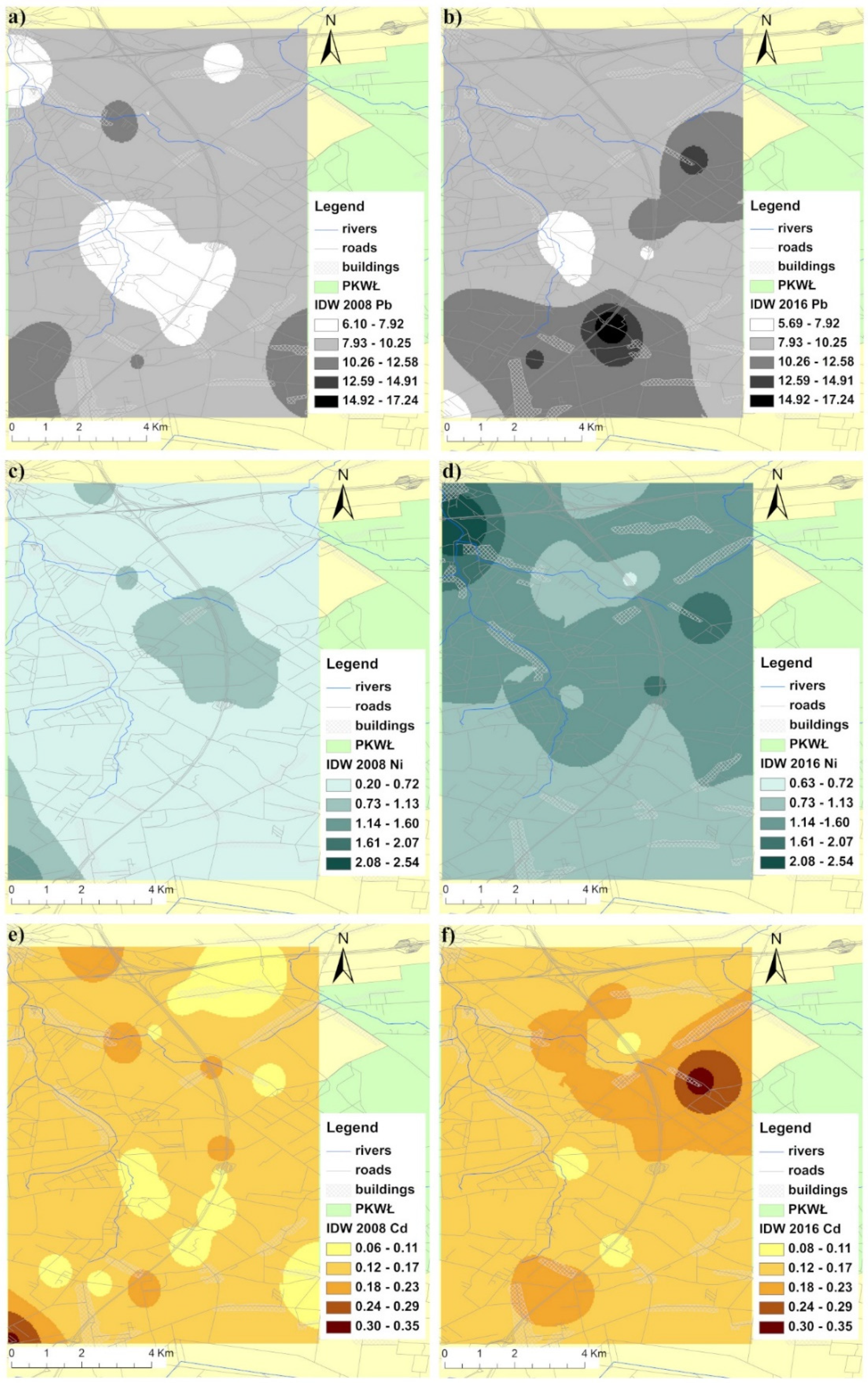
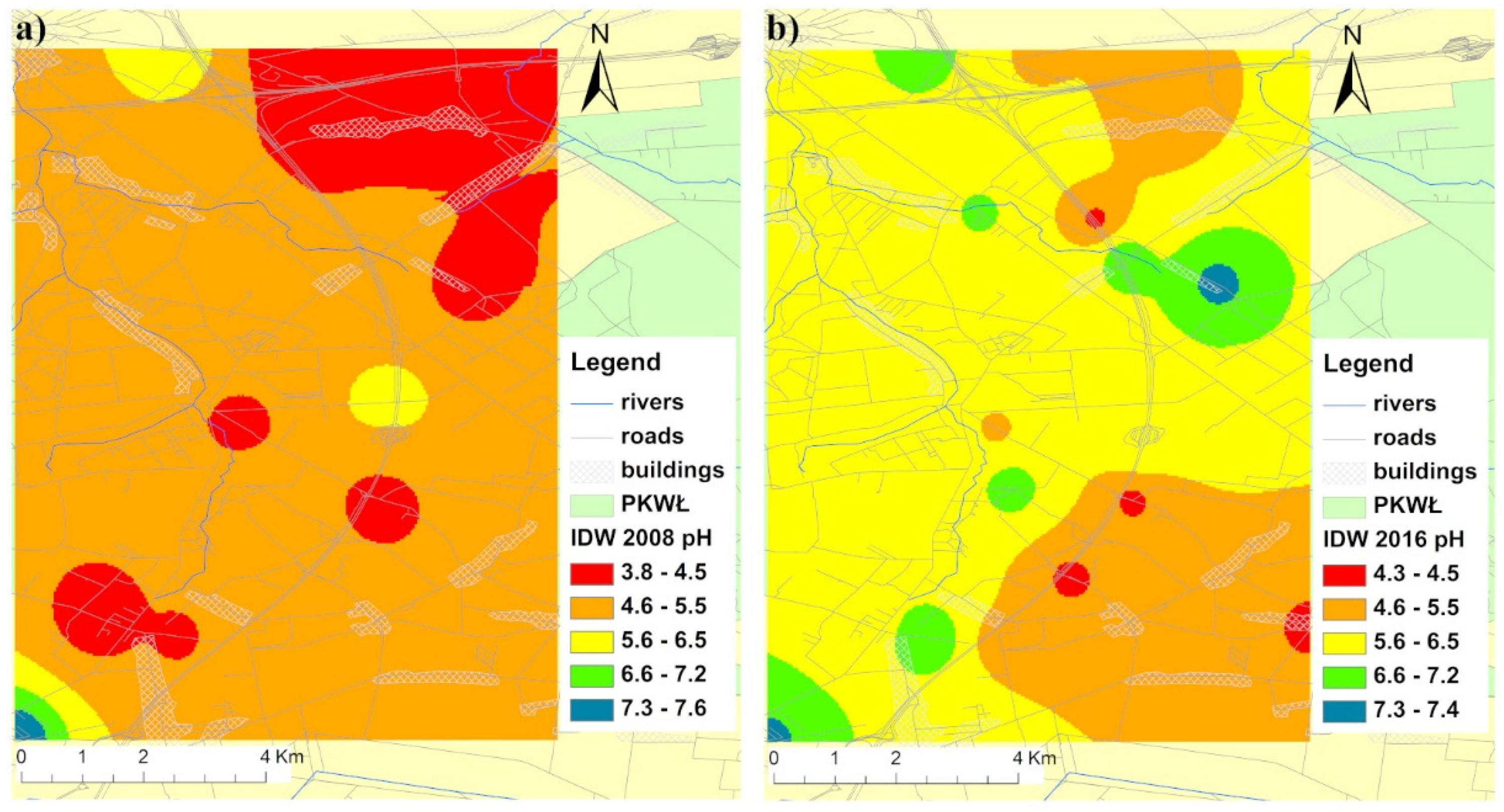
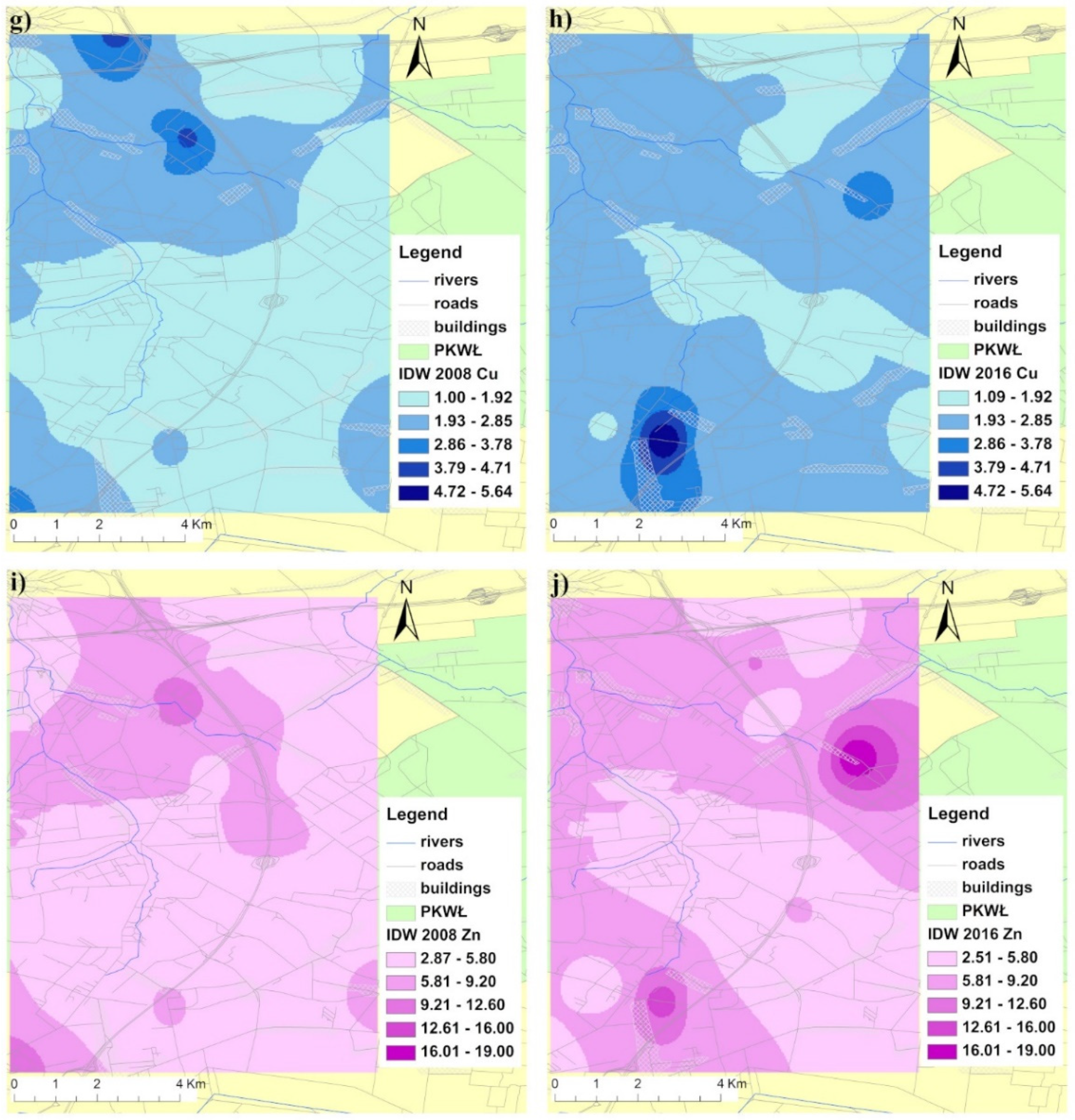
3.1. Soil Characterization and Metal Distribution Maps
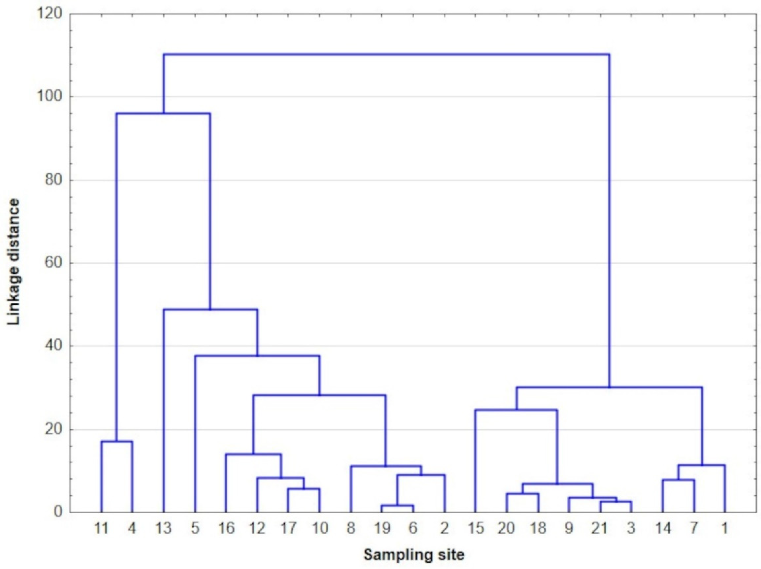
3.2. Principal Component Analysis (PCA) and Cluster Analysis (CA)
4. Conclusions
Supplementary Materials
Author Contributions
Funding
Data Availability Statement
Acknowledgments
Conflicts of Interest
References
- Dudley, N. (Ed.) Guidelines for Applying Protected Area Management Categories; IUCN: Gland, Switzerland, 2008; Available online: https://www.iucn.org/theme/protected-areas/about/protected-area-categories (accessed on 5 May 2022).
- The Act on Nature Conservation. Journal of Law of 2022, Item 916. Available online: https://isap.sejm.gov.pl/isap.nsf/DocDetails.xsp?id=WDU20220000916 (accessed on 5 May 2022). (In Polish)
- Karpus, K. Legal protection of landscape in Poland in the light of the Act of 24 April 2015 amending certain acts in relation to strenghtening landscape protection instruments. Pol. Yearb. Environ. Law 2016, 6, 57–79. [Google Scholar] [CrossRef] [Green Version]
- Szczepańska, M.; Wilkaniec, A.; Škamlova, L. Visual Pollution in Natural and Landscape Protected Areas: Case Study from Poland and Slovakia. Quaest. Geogr. 2019, 38, 133–149. [Google Scholar] [CrossRef] [Green Version]
- Kot-Niewiadomska, A.; Pawłowska, A. The Possibilities of Open-Cast Mining in Landscape Parks in Poland—A Case Study. Resources 2020, 9, 122. [Google Scholar] [CrossRef]
- The Marshal of the Sejm of the Republic of Poland. Announcement of the Marshal of the Sejm of the Republic of Poland of 11 March 2022 on the announcement of the consolidated text of the Nature Conservation Act. In Journal of Laws of 2022, Item 916; Wydawnictwo Sejmowe: Warsaw, Poland, 2022. [Google Scholar]
- Wycichowska, B. Appropriating protected cultural landscape by gmina self-governments and its negative effects-example of the Wzniessienia Łódzkie Landscape Park. Diss. Curtural Landsc. Comm. 2008, 10, 368–376. Available online: http://krajobraz.kulturowy.us.edu.pl/publikacje.artykuly/zarzadzanie/wycichowska.pdf (accessed on 5 May 2022).
- Hansen, A.S. Understanding recreational landscape—A review and discussion. Landsc. Res. 2021, 46, 128–141. [Google Scholar] [CrossRef]
- Drzazga, D.; Ratajczyk, N. Suburban sprawl of Łódź agglomeration within Łódź Hills Landscape Park. Przegląd Przyr. 2005, 16, 183–199. [Google Scholar]
- Wojdan, D. The preliminary assessment of road renovation impact in the nature of the Świętokrzyski National Park. Prądnik. Prace Muz. Szefera 2010, 20, 441–452. Available online: http://www.ojcowskiparknarodowy.pl/main/pradnik.html (accessed on 5 May 2022).
- Trombulak, S.C.; Frissell, C.A. Review of Ecological Effects of Roads on Terrestrial and Aquatic Communities. Conserv. Biol. 2000, 14, 18–30. [Google Scholar] [CrossRef]
- Şakar, D.; Aydin, A.; Akay, A.E. Essential Issues Related to Construction Phases of Road Networks in Protected Areas: A Review. Croat. J. For. Eng. 2022, 43, 219–237. [Google Scholar] [CrossRef]
- Kozak, M.; Pudełko, R. Impact Assessment of the Long-Term Fallowed Land on Agricultural Soils and the Possibility of Their Return to Agriculture. Agriculture 2021, 11, 148. [Google Scholar] [CrossRef]
- Radzimska, M.; Fronczyk, J. Level and Contamination Assessment of Soil along an Expressway in an Ecologically Valuable Area in Central Poland. Int. J. Environ. Res. Public Health 2015, 12, 13372–13387. [Google Scholar] [CrossRef] [PubMed] [Green Version]
- Mazurek, R.; Kowalska, J.; Gąsiorek, M.; Zadrożny, P.; Józefowska, A.; Zaleski, T.; Kępka, W.; Tymczuk, M.; Orłowska, K. Assessment of heavy metals contamination in surface layers of Roztocze National Park forest soils (SE Poland) by indices of pollution. Chemosphere 2017, 168, 839–850. [Google Scholar] [CrossRef] [PubMed]
- Huang, J.; Wu, Y.; Li, Y.; Sun, J.; Xie, Y.; Fan, Z. Do trace metal(oid)s in road soils pose health risks to tourists? A case of a highly-visited national park in China. J. Environ. Sci. 2022, 111, 61–74. [Google Scholar] [CrossRef] [PubMed]
- Słowik, T.; Jackowska, I.; Piekarski, W. The environment pollution problems caused by the transport infrastructure at the sample of the Roztocze National Park. Acta Agroph. 2008, 5, 1–138. Available online: http://www.acta-agrophysica.org/Problemy-zanieczyszczenia-srodowiska-przez-infrastrukture-transportowa-na-przykladzie,148229,0,2.html (accessed on 5 May 2022).
- Huang, Z.; Liu, K.; Duan, J.; Wang, Q. A review of waste-containing building materials: Characterization of the heavy metal. Constr. Build. Mater. 2021, 309, 125107. [Google Scholar] [CrossRef]
- Zhao, Y.; Zu, Y.T. Metals Leaching in Permeable Asphalt Pavement with Municipal Solid Waste Ash Aggregate. Water 2019, 11, 2186. [Google Scholar] [CrossRef] [Green Version]
- Różański, S.; Jaworska, H.; Matuszczak, K.; Nowak, J.; Hardy, A. Impact of highway traffic and the acoustic screen on the content and spatial distribution of heavy metals in soils. Environ. Sci. Pollut. Res. 2017, 24, 12778–12786. [Google Scholar] [CrossRef] [Green Version]
- Ličbinský, R.; Huzlik, J.; Provalilová, I.; Jandová, V.; Ličbinská, M. Groundwater Contamination Caused by Road Construction Materials. Trans. Transp. Sci. 2012, 5, 205–2014. [Google Scholar] [CrossRef] [Green Version]
- Kalarus, D.; Baran, T.; Ostrowski, M. Influence of secondary fuel components used in the manufacture of Portland cement clinker to the value of heavy metal emissions from cement and concrete. Prace ICMB 2016, 25, 7–17. Available online: https://icimb.home.pl/opole/wydawnictwa/prace-icimb/434 (accessed on 5 May 2022).
- Jaskulski, M.; Schmidt, A. The tourism attractiveness of landforms in Łagiewnicki forest, Łódź. Tourism 2015, 25/2, 27–35. [Google Scholar] [CrossRef] [Green Version]
- Kurowski, J.K.; Papińska, E.; Andrzejewski, H. Atlas of Łódź. Sheet XIII: Sozology—Selected Issues of Environmental Protection and Degradation. Available online: http://mapa.lodz.pl/mapa/atlas/eng/en-13R.pdf (accessed on 5 May 2022).
- Ecophysiographic Study. Łódź, Poland. 2018. Available online: http://docplayer.pl/136706965-Opracowanie-ekofizjograficzne.html (accessed on 5 May 2022). (In Polish).
- Rdzany, Z. Geographical location and regional diversity of Poland. In Natural Environment of Poland and Its Protection, 1st ed.; Kobojek, E., Marszał, T., Eds.; Łódź University Press: Łódź, Poland, 2014; pp. 9–40. [Google Scholar]
- Polish Committee for Standarization. Polish Standard (1998). PN-R-04032:1998; Soil and Mineral Grounds. Soil Sampling and Grain Size Distribution. PKN: Warsaw, Poland, 1998.
- Polish Committee for Standarization. Polish Standard (2001). PN-ISO-11259 (2001); Soil Quality—Simplified Soil Description. PKN: Warsaw, Poland, 2001.
- Caravaca, F.; Lozano, Z.; Rodriguez-Caballero, G.; Roldán, A. Spatial shifts in soil microbial activity and degradation of pasture civer caused by prolonged exposure to cement dust. Land Degrad. Dev. 2017, 28, 1329–1335. [Google Scholar] [CrossRef]
- Polish Committee for Standarization. Polish Standard (2005). PN-ISO 10390:2005; Soil Quality—Determination of pH. PKN: Warsaw, Poland, 2005.
- Polish Committee for Standarization. Polish Standard. PN-R-04016:1992; Agrochemical Soil Analyses—Determination of Assimilated Zinc Contents. PKN: Warsaw, Poland, 1992.
- Polish Committee for Standarization. Polish Standard. PN-R-04017:1992; Agrochemical Soil Analyses—Determination of Assimilated Copper Contents. PKN: Warsaw, Poland, 1992.
- Bąbelewska, A. The impact of industrial emissions on heavy metal and sulphur contamination level within the area of the projected Jurassic National Park. Prądnik Stud. Rep. Prof. Władysław Szafer Mus. 2010, 20, 135–145. [Google Scholar]
- Weber, C.J.; Santowski, A.; Chifflard, P. Spatial variability in heavy metal concentration in urban pavement joints—A case study. Soil 2021, 7, 15–31. [Google Scholar] [CrossRef]
- Head Office of Geodesy and Cartography. Available online: www.gugik.gov.pl (accessed on 27 April 2022).
- Xie, Y.F.; Chen, T.B.; Lei, M.; Yang, J.; Guo, Q.J.; Song, B.; Zhou, X.Y. Spatial distribution of soil heavy metal pollution estimated by different interpolation methods: Accuracy and uncertainty analysis. Chemosphere 2011, 82, 468–476. [Google Scholar] [CrossRef]
- Kelepertzis, E. Accumulation of heavy metals in agricultural soils of Mediterranean: Insights from Argolida basin, Peloponnese, Greece. Geoderma 2014, 221–222, 82–90. [Google Scholar] [CrossRef]
- Rodriguez-Seijo, A.; Andrade, M.L.; Vega, F.A. Origin and spatial distribution of metals in urban soils. J. Soils Sediments 2017, 17, 1514–1526. [Google Scholar] [CrossRef]
- Siebielec, G.; Łopatka, A.; Smreczek, B.; Kaczyński, R.; Siebielec, S.; Koza, P.; Dach, J. Materia organiczna w glebach mineralnych Polski. Stud. Rap. IUNG-PIB 2020, 64, 9–30. [Google Scholar] [CrossRef]
- Kissel, D.E.; Bock, B.R.; Ogles, C.Z. Thoughts on acidification of soils by nitrogen and sulfur fertilizers. Agrosyst. Geosci. Environ. 2020, 3, e20060. [Google Scholar] [CrossRef]
- Vašák, F.; Černý, J.; Buráňová, Š.; Kulhánek, M.; Balík, J. Soil pH Changes in Long-Term Field Experiments with Different Fertilizing Systems. Soil Water Res. 2015, 10, 19–23. [Google Scholar] [CrossRef] [Green Version]
- Naveen, B.P.; Mahapatra, D.M.; Sitharam, T.G.; Sivapullaiah, P.V.; Ramachandra, T.V. Physico-chemical and biological characterization of urban municipal landfill leachate. Environ. Pollut. 2017, 220, 1–12. [Google Scholar] [CrossRef]
- Oka, G.A.; Thomas, L.; Lavkulich, L.M. Soil assessment for urban agriculture: A Vancouver case study. J. Soil Sci. Plant Nut. 2014, 14, 657–669. [Google Scholar] [CrossRef] [Green Version]
- Senila, M. Real and simulated bioavailability of lead in contaminated and uncontaminated soils. J. Environ. Health Sci. Eng. 2014, 12, 108. [Google Scholar] [CrossRef] [PubMed] [Green Version]
- Kwon, M.J.; Boyanov, M.I.; Yang, J.S.; Lee, S.; Hwang, Y.H.; Lee, J.Y.; Mishra, B.; Kemner, K.M. Transformation of zinc-concentrate in surface and subsurface environments: Implications for assessing zinc mobility/toxicity and choosing an optimal remediation strategy. Environ. Pollut. 2017, 226, 346–355. [Google Scholar] [CrossRef]
- Senila, M.; Levei, E.A.; Senila, L.R. Assessment of metals bioavailability to vegetables under field conditions using DGT, single extractions and multivariate statistics. Chem. Cent. J. 2012, 6, 119. [Google Scholar] [CrossRef] [PubMed] [Green Version]
- Jezierski, P.; Jagodzik, W. The risk evaluation of arable land of heavy metals pollution as an outcome of metallurgical slug applied to the solid-surfaced roads hardening. Ochr. Śr. Zasobów Nat. 2010, 42, 158–166. Available online: http://agro.icm.edu.pl/agro/element/bwmeta1.element.agro-be78ff50-1117-4691-994f-dbb1df01a93a (accessed on 5 May 2022).
- Minister of the Environment. Regulation of the Minister of the Environment of 1 September 2016 on the Method of the Contamination Assessment of the Earth Surface. In Journal of Laws of 2016, Item 1395; Wydawnictwo Sejmowe: Warsaw, Poland, 2016. [Google Scholar]
- Hui, Z.; Caiqiu, W.; Jiping, G.; Xuyin, Y.; Qiao, W.; Wenming, P.; Tao, L.; Jie, Q.; Hanpei, Z. Assessment of Heavy Metal Contamination in Roadside Soils Along the Shenyang-Dalian Highway in Liaoning Province, China. Pol. J. Environ. Stud. 2017, 26, 1539–1549. [Google Scholar] [CrossRef]
- Karim, Z.; Qureshi, B.A.; Mumtaz, M.; Qureshi, S. Heavy metal content in urban soils as an indicator of anthropogenic and natural influences on landscape of Karachi—A multivariate spatio-temporal analysis. Ecol. Indic. 2014, 42, 20–31. [Google Scholar] [CrossRef]
- Schober, P.; Boer, C.; Schwarte, L.A. Correlation coefficients: Appropriate Use and Interpretation. Anesth. Analg. 2018, 126, 1763–1768. [Google Scholar] [CrossRef]
- Hjortenkrans, D. Road Traffic Metals—Sources and Emissions. Ph.D. Thesis, University of Kalmar, Kalmar, Sweden, 2008. [Google Scholar]
- Athanasopoulou, A.; Kollaros, G. Heavy Metal Contamination of Soil Due to Road Traaffic. Am. J. Eng. Res. 2016, 5, 354–363. [Google Scholar]
- Skorbiłowicz, M.; Skorbiłowicz, E.; Łapiński, W. Assessment of Metallic Content, Pollution, and Sources of Road Dust in the City of Białystok (Poland). Aerosol Air Qual. Res. 2020, 20, 2507–2518. [Google Scholar] [CrossRef]
- Alengebawy, A.; Abdelkhalek, S.T.; Qureshi, S.R.; Wang, M.-Q. Heavy Metals and Pesticides in Agricultural Soil and Plants: Ecological Risks and Human Health Implications. Toxics 2021, 9, 42. [Google Scholar] [CrossRef] [PubMed]
- Wang, J.; Ju, D.; Wang, Y.; Du, X.; Li, G.; Li, B.; Zhao, Y.; Wei, Y.; Xu, S. Source analysis of heavy metal pollution in agriculture soil irrigated with sewage in Wuqing, Tianjin. Sci. Rep. 2021, 11, 17816. [Google Scholar] [CrossRef]
- Nakamura, K.; Kuwatani, T.; Kawabe, Y.; Komai, T. Extraction of heavy metals characteristics of the 2011 Tohoku tsunami deposits using multiple classification analysis. Chemosphere 2016, 144, 1241–1248. [Google Scholar] [CrossRef] [PubMed] [Green Version]
- Facchianelli, A.; Sacchi, E.; Mallen, L. Multivariate statistical and GIS-based approach to identify heavy metal sources in soils. Environ. Pollut. 2001, 114, 313–324. [Google Scholar] [CrossRef]
- Sherene, T. Mobility and transport of heavy metals in polluted soil environment. Biol. Forum Int. J. 2010, 2, 112–121. [Google Scholar]
- Ren, Z.; Sivry, Y.; Tharaud, M.; Cordier, L.; Li, Y.; Dai, J.; Benedetti, M.F. Speciation and reactivity of lead and zinc in heavily and poorly contaminated soils: Stable isotope dilution, chemical extraction and model views. Environ. Pollut. 2017, 225, 654–662. [Google Scholar] [CrossRef]
- Sutherland, R.A. Bed sediment-associated trace metals in an urban stream, Oahu, Hawaii. Environ. Geol. 2000, 39, 611–627. [Google Scholar] [CrossRef]


| No. | Latitude | Longitude | Site Feature | pH-H2O | pH-KCl | Organic Matter [%] | Textural Classification [27,28] | ||||
|---|---|---|---|---|---|---|---|---|---|---|---|
| 2008 | 2016 | 2008 | 2016 | 2008 | 2016 | 2008 | 2016 | 2008/2016 | |||
| 1 | 51°53′17″ N | 19°36′31″ E | grassland | grassland | 6.3 | 6.2 | 4.9 | 5.7 | 5.1 | 5.3 | sandy loam |
| 2 | 51°53′55″ N | 19°37′34″ E | cropland | fallow (1) | 7.0 | 7.1 | 6.4 | 6.9 | 2.9 | 3.2 | sandy loam |
| 3 | 51°53′52″ N | 19°38′37″ E | cropland | cropland | 5.7 | 6.3 | 4.1 | 5.3 | 3.8 | 3.7 | sandy loam |
| 4 | 51°51′51″ N | 19°40′11″ E | cropland | cropland | 5.7 | 7.5 | 4.2 | 7.4 | 4.4 | 4.3 | sandy loam |
| 5 | 51°52′35″ N (a) 51°52′25″ N (b) | 19°38′27″ E (a) 19°39′07″ E (b) | pasture | cropland | 5.9 | 5.4 | 4.8 | 4.3 | 3.3 | 3.0 | sandy loam |
| 6 | 51°52′04″ N | 19°39′21″ E | cropland | cropland | 6.5 | 7.2 | 5.2 | 7.0 | 3.6 | 3.7 | sandy loam |
| 7 | 51°53′04″ N | 19°38′52″ E | fallow (1) | fallow (2) | 5.4 | 6.6 | 3.8 | 6.0 | 4.5 | 4.3 | sandy loam |
| 8 | 51°50′44″ N | 19°39′29″ E | fallow (1) | fallow (1) | 7.3 | 6.5 | 6.4 | 6.1 | 3.9 | 4.5 | sandy loam |
| 9 | 51°50′34″ N | 19°38′14″ E | grassland | grassland | 5.8 | 6.1 | 4.2 | 5.4 | 3.3 | 3.1 | sand |
| 10 | 51°48′41″ N | 19°38′16″ E | fallow (1) | fallow (3) | 6.5 | 6.0 | 5.0 | 5.1 | 3.8 | 4.5 | loamy sand |
| 11 | 51°48′43″ N | 19°37′40″ E | cropland | fallow (1) | 5.8 | 7.0 | 4.4 | 7.0 | 3.5 | 3.8 | loamy sand |
| 12 | 51°48′53″ N | 19°36′56″ E | cropland | cropland | 5.4 | 6.6 | 4.1 | 6.1 | 4.2 | 4.1 | loamy sand |
| 13 | 51°47′49″ N | 19°36′13″ E | fallow (1) | fallow (2) | 8.0 | 7.3 | 7.6 | 7.3 | 3.3 | 3.0 | loamy sand |
| 14 | 51°50′03″ N | 19°38′22″ E | cropland | cropland | 6.6 | 7.1 | 5.3 | 6.9 | 3.2 | 3.0 | loamy sand |
| 15 | 51°49′14″ N (a) 51°49′15″ N (b) | 19°38′56″ E (a) 19°38′53″ E (b) | cropland | fallow (1) | 6.1 | 5.4 | 4.7 | 4.3 | 3.8 | 4.0 | sandy loam |
| 16 | 51°48′49″ N | 19°40′59″ E | cropland | cropland | 6.4 | 5.6 | 5.1 | 4.4 | 3.8 | 3.7 | loamy sand |
| 17 | 51°52′29″ N | 19°38′06″ E | cropland | cropland | 6.0 | 6.9 | 4.7 | 6.6 | 3.3 | 3.4 | loamy sand |
| 18 | 51°53′21″ N | 19°39′37″ E | cropland | cropland | 5.1 | 5.7 | 3.8 | 4.5 | 3.6 | 3.7 | sandy loam |
| 19 | 51°51′41″ N | 19°38′49″ E | cropland | cropland | 5.3 | 7.1 | 5.2 | 6.5 | 4.0 | 4.0 | sandy loam |
| 20 | 51°49′56″ N | 19°39′26″ E | fallow (1) | fallow (1) | 5.5 | 5.5 | 4.0 | 4.3 | 3.6 | 5.6 | sandy loam |
| 21 | 51°50′24″ N | 19°39′28″ E | fallow (1) | fallow (1) | 5.9 | 6.8 | 4.8 | 6.3 | 2.6 | 2.9 | sandy loam |
| No. | Zn [mg/kg] | Cu [mg/kg] | Pb [mg/kg] | Cd [mg/kg] | Ni [mg/kg] | Sj | ||||||
|---|---|---|---|---|---|---|---|---|---|---|---|---|
| 2008 | 2016 | 2008 | 2016 | 2008 | 2016 | 2008 | 2016 | 2008 | 2016 | 2008 | 2016 | |
| 1 | 3.40 | 7.54 | 1.48 | 2.39 | 7.10 | 8.43 | 0.12 | 0.17 | 0.32 | 2.50 | −1.52 | 1.40 |
| 2 | 7.80 | 6.20 | 3.98 | 2.11 | 10.1 | 9.66 | 0.22 | 0.14 | 0.80 | 1.23 | 2.29 | −0.08 |
| 3 | 4.18 | 2.64 | 1.51 | 1.44 | 8.31 | 8.28 | 0.12 | 0.11 | 0.47 | 0.76 | −1.00 | −1.70 |
| 4 | 4,50 | 19.0 | 1.70 | 3.32 | 9.50 | 13.5 | 0.10 | 0.32 | 0.70 | 1.90 | −0.51 | 4.65 |
| 5 | 11.9 | 3.42 | 4.10 | 1.20 | 7.90 | 8.02 | 0.10 | 0.08 | 0.40 | 0.63 | 1.31 | −2.02 |
| 6 | 6.51 | 6.21 | 2.42 | 2.10 | 9.13 | 9.23 | 0.18 | 0.18 | 0.75 | 1.40 | 0.81 | 0.27 |
| 7 | 5.60 | 9.50 | 1.40 | 2.17 | 8.10 | 8.75 | 0.10 | 0.20 | 0.70 | 1.46 | −0.62 | 0.96 |
| 8 | 8.40 | 5.02 | 1.70 | 2.32 | 9.00 | 12.1 | 0.20 | 0.20 | 1.10 | 1.78 | 1.46 | 0.94 |
| 9 | 3.40 | 3.23 | 1.00 | 1.09 | 6.10 | 5.69 | 0.10 | 0.09 | 0.40 | 1.11 | −1.89 | −1.87 |
| 10 | 6.30 | 6.67 | 2.00 | 2.12 | 10.4 | 11.9 | 0.20 | 0.19 | 0.60 | 0.87 | 0.63 | 0.25 |
| 11 | 4.20 | 14.5 | 1.90 | 5.51 | 8.70 | 12.8 | 0.10 | 0.20 | 0.40 | 1.02 | −1.02 | 3.38 |
| 12 | 5.10 | 4.66 | 1.90 | 1.74 | 11.1 | 11.2 | 0.10 | 0.15 | 0.70 | 0.96 | −0.13 | −0.51 |
| 13 | 11.4 | 4.99 | 3.10 | 1.95 | 12.0 | 6.42 | 0.30 | 0.11 | 1.50 | 0.83 | 4.35 | −1.21 |
| 14 | 3.60 | 5.27 | 1.50 | 2.37 | 6.90 | 7.31 | 0.10 | 0.13 | 0.50 | 1.32 | −1.36 | −0.34 |
| 15 | 3.20 | 2.88 | 1.10 | 1.99 | 7.40 | 17.2 | 0.10 | 0.09 | 0.70 | 1.04 | −1.26 | −0.37 |
| 16 | 6.10 | 4.03 | 2.30 | 1.80 | 12.4 | 8.61 | 0.10 | 0.12 | 0.20 | 1.07 | −0.39 | −0.95 |
| 17 | 9.17 | 7.41 | 2.72 | 2.28 | 12.1 | 10.2 | 0.21 | 0.19 | 0.78 | 0.89 | 2.02 | 0.28 |
| 18 | 2.87 | 3.71 | 1.34 | 1.56 | 7.53 | 8.74 | 0.06 | 0.11 | 0.29 | 1.15 | −2.11 | −1.09 |
| 19 | 5.33 | 6.24 | 2.62 | 2.32 | 8.81 | 9.71 | 0.17 | 0.20 | 0.99 | 1.17 | 0.97 | 0.37 |
| 20 | 5.70 | 6.23 | 1.40 | 1.57 | 7.80 | 8.56 | 0.10 | 0.14 | 0.70 | 0.96 | −0.64 | −0.67 |
| 21 | 3.20 | 2.51 | 1.45 | 1.26 | 7.20 | 7.40 | 0.10 | 0.11 | 0.52 | 1.01 | −1.39 | −1.68 |
| Range [mg/kg] | 2.87–11.9 | 2.51–19.0 | 1.00–4.10 | 1.09–5.51 | 6.10–12.4 | 5.69–17.2 | 0.06–0.30 | 0.80–0.32 | 0.20–1.50 | 0.62–2.50 | ||
| Mean [mg/kg] | 5.80 | 6.28 | 2.03 | 2.12 | 8.94 | 9.70 | 0.14 | 0.15 | 0.64 | 1.19 | ||
| Median [mg/kg] | 5.33 | 5.27 | 1.70 | 2.10 | 8.70 | 8.75 | 0.10 | 0.14 | 0.70 | 1.07 | ||
| S−W Test (p) | 0.02 | 0.00 | 0.01 | 0.00 | 0.20 | 0.09 | 0.00 | 0.02 | 0.08 | 0.01 | ||
| CV [%] | 45.2 | 63.5 | 42.6 | 43.7 | 20.4 | 27.5 | 43.5 | 36.5 | 46.7 | 36.2 | ||
| No. | Zn [mg/kg] | Cu [mg/kg] | Pb [mg/kg] | Cd [mg/kg] | Ni [mg/kg] | ||||||
|---|---|---|---|---|---|---|---|---|---|---|---|
| 2008 | 2016 | 2008 | 2016 | 2008 | 2016 | 2008 | 2016 | 2008 | 2016 | ||
| 1 | CF | 0.75 | 0.80 | 0.61 | 1.24 | 1.99 | 2.23 | 8.15 | 11.83 | 1.21 | 2.81 |
| EF | 1.77 | 1.13 | 1.44 | 1.76 | 4.70 | 3.16 | 19.31 | 16.78 | 2.86 | 3.99 | |
| Igeo | −1.00 | −0.91 | −0.39 | −0.08 | 0.41 | 0.57 | 0.74 | 0.90 | −0.32 | 0.91 | |
| 2 | CF | 1.19 | 1.43 | 1.14 | 2.52 | 2.12 | 2.24 | 8.00 | 17.30 | 2.12 | 2.07 |
| EF | 1.90 | 3.28 | 1.81 | 5.78 | 3.38 | 5.14 | 12.76 | 39.77 | 3.37 | 4.77 | |
| Igeo | −0.33 | −0.07 | −0.12 | 0.22 | 0.50 | 0.58 | 0.73 | 1.06 | 0.50 | 0.47 | |
| 3 | CF | 0.62 | 0.41 | 1.20 | 0.93 | 1.48 | 1.63 | 7.89 | 10.18 | 1.68 | 1.90 |
| EF | 1.38 | 0.92 | 2.66 | 2.09 | 3.29 | 3.66 | 17.48 | 22.78 | 3.73 | 4.25 | |
| Igeo | −1.27 | −1.87 | −0.10 | −0.21 | −0.02 | 0.12 | 0.72 | 0.83 | 0.16 | 0.34 | |
| 4 | CF | 1.09 | 1.39 | 1.58 | 1.42 | 1.74 | 2.16 | 11.29 | 11.31 | 3.38 | 3.69 |
| EF | 1.45 | 2.39 | 2.10 | 2.43 | 2.30 | 3.72 | 14.99 | 19.47 | 4.49 | 6.35 | |
| Igeo | −0.46 | −0.11 | 0.02 | −0.03 | 0.21 | 0.53 | 0.88 | 0.88 | 1.17 | 1.30 | |
| 5 | CF | 1.26 | 0.41 | 0.67 | 0.88 | 1.82 | 1.96 | 8.28 | 13.80 | 1.63 | 1.79 |
| EF | 2.56 | 1.09 | 1.36 | 2.35 | 3.72 | 5.22 | 16.89 | 36.72 | 3.32 | 4.76 | |
| Igeo | −0.26 | −1.88 | −0.35 | −0.23 | 0.28 | 0.39 | 0.74 | 0.96 | 0.12 | 0.25 | |
| 6 | CF | 1.08 | 0.86 | 0.94 | 1.14 | 2.20 | 2.12 | 10.66 | 12.46 | 1.43 | 2.55 |
| EF | 1.78 | 1.29 | 1.54 | 1.70 | 3.62 | 3.17 | 17.58 | 18.64 | 2.35 | 3.82 | |
| Igeo | −0.48 | −0.79 | −0.20 | −0.12 | 0.55 | 0.50 | 0.85 | 0.92 | −0.07 | 0.77 | |
| 7 | CF | 0.74 | 1.08 | 0.46 | 1.26 | 1.84 | 2.34 | 8.73 | 13.10 | 1.20 | 2.20 |
| EF | 1.67 | 1.70 | 1.05 | 1.98 | 4.17 | 3.68 | 19.80 | 20.59 | 2.72 | 3.45 | |
| Igeo | −1.02 | −0.47 | −0.51 | −0.08 | 0.29 | 0.64 | 0.77 | 0.94 | −0.32 | 0.55 | |
| 8 | CF | 1.46 | 0.88 | 0.97 | 1.18 | 3.04 | 4.00 | 8.10 | 11.31 | 1.65 | 2.40 |
| EF | 2.21 | 1.09 | 1.47 | 1.46 | 4.61 | 4.98 | 12.27 | 14.08 | 2.51 | 2.99 | |
| Igeo | −0.04 | −0.77 | −0.19 | −0.11 | 1.02 | 1.42 | 0.73 | 0.88 | 0.14 | 0.68 | |
| 9 | CF | 0.76 | 0.60 | 0.99 | 0.77 | 2.41 | 2.28 | 4.44 | 10.58 | 1.62 | 1.82 |
| EF | 1.79 | 1.45 | 2.33 | 1.87 | 5.70 | 5.51 | 10.53 | 25.63 | 3.83 | 4.42 | |
| Igeo | −0.99 | −1.32 | −0.18 | −0.29 | 0.68 | 0.60 | 0.47 | 0.85 | 0.11 | 0.28 | |
| 10 | CF | 1.11 | 1.11 | 0.94 | 1.35 | 3.24 | 3.55 | 12.02 | 13.47 | 1.48 | 2.18 |
| EF | 1.46 | 1.59 | 1.23 | 1.93 | 4.26 | 5.07 | 15.81 | 19.24 | 1.95 | 3.11 | |
| Igeo | −0.43 | −0.43 | −0.20 | −0.04 | 1.11 | 1.24 | 0.90 | 0.95 | −0.02 | 0.54 | |
| 11 | CF | 0.89 | 1.81 | 0.53 | 1.48 | 2.22 | 2.16 | 9.73 | 12.22 | 1.13 | 2.14 |
| EF | 2.03 | 2.75 | 1.21 | 2.26 | 5.06 | 3.30 | 22.16 | 18.62 | 2.58 | 3.25 | |
| Igeo | −0.75 | 0.27 | −0.45 | −0.01 | 0.57 | 0.53 | 0.81 | 0.91 | −0.41 | 0.51 | |
| 12 | CF | 0.82 | 0.65 | 0.88 | 0.95 | 2.45 | 2.23 | 9.51 | 12.34 | 1.30 | 1.92 |
| EF | 1.80 | 1.23 | 1.93 | 1.79 | 5.34 | 4.21 | 20.78 | 23.26 | 2.83 | 3.62 | |
| Igeo | −0.87 | −1.21 | −0.23 | −0.20 | 0.71 | 0.57 | 0.80 | 0.92 | −0.21 | 0.36 | |
| 13 | CF | 1.83 | 0.46 | 1.85 | 1.27 | 3.96 | 3.35 | 10.10 | 16.14 | 2.28 | 2.80 |
| EF | 2.47 | 0.94 | 2.51 | 2.59 | 5.36 | 6.80 | 13.67 | 32.76 | 3.09 | 5.68 | |
| Igeo | 0.28 | −1.69 | 0.09 | −0.07 | 1.40 | 1.16 | 0.83 | 1.03 | 0.60 | 0.90 | |
| 14 | CF | 0.87 | 0.86 | 0.77 | 1.51 | 1.96 | 1.83 | 8.68 | 14.41 | 1.46 | 2.76 |
| EF | 1.82 | 1.25 | 1.62 | 2.18 | 4.12 | 2.65 | 18.27 | 20.85 | 3.08 | 3.99 | |
| Igeo | −0.79 | −0.80 | −0.29 | 0.00 | 0.38 | 0.29 | 0.76 | 0.98 | −0.03 | 0.88 | |
| 15 | CF | 0.88 | 1.03 | 1.28 | 1.55 | 1.68 | 2.45 | 4.44 | 6.94 | 1.68 | 2.05 |
| EF | 1.21 | 1.80 | 1.76 | 2.71 | 2.30 | 4.28 | 6.10 | 12.14 | 2.31 | 3.58 | |
| Igeo | −0.77 | −0.54 | −0.07 | 0.01 | 0.16 | 0.71 | 0.47 | 0.67 | 0.16 | 0.45 | |
| 16 | CF | 1.08 | 1.00 | 0.94 | 1.17 | 2.33 | 2.18 | 11.79 | 13.00 | 1.75 | 2.73 |
| EF | 1.62 | 1.75 | 1.40 | 2.04 | 3.48 | 3.80 | 17.61 | 22.71 | 2.62 | 4.77 | |
| Igeo | −0.47 | −0.58 | −0.20 | −0.11 | 0.63 | 0.54 | 0.90 | 0.94 | 0.23 | 0.86 | |
| 17 | CF | 0.99 | 0.99 | 0.72 | 1.27 | 2.16 | 1.44 | 11.79 | 13.61 | 1.31 | 1.71 |
| EF | 2.33 | 2.45 | 1.69 | 3.14 | 5.10 | 3.57 | 27.84 | 33.76 | 3.10 | 4.25 | |
| Igeo | −0.60 | −0.60 | −0.32 | −0.07 | 0.53 | −0.06 | 0.90 | 0.96 | −0.19 | 0.19 | |
| 18 | CF | 0.50 | 0.58 | 0.57 | 0.94 | 1.84 | 2.04 | 7.89 | 10.56 | 1.45 | 1.96 |
| EF | 1.48 | 1.47 | 1.71 | 2.39 | 5.49 | 5.16 | 23.56 | 26.70 | 4.32 | 4.97 | |
| Igeo | −1.60 | −1.37 | −0.42 | −0.20 | 0.29 | 0.44 | 0.72 | 0.85 | −0.05 | 0.39 | |
| 19 | CF | 0.82 | 1.01 | 0.55 | 1.18 | 1.77 | 1.81 | 9.68 | 9.00 | 1.91 | 1.83 |
| EF | 2.09 | 2.20 | 1.40 | 2.57 | 4.53 | 3.93 | 24.76 | 19.55 | 4.87 | 3.97 | |
| Igeo | −0.88 | −0.57 | −0.44 | −0.10 | 0.24 | 0.27 | 0.81 | 0.78 | 0.34 | 0.29 | |
| 20 | CF | 0.63 | 0.81 | 0.60 | 0.99 | 1.66 | 1.59 | 2.85 | 9.94 | 1.51 | 2.12 |
| EF | 1.31 | 1.79 | 1.26 | 2.19 | 3.48 | 3.53 | 5.95 | 22.00 | 3.16 | 4.68 | |
| Igeo | −1.25 | −0.89 | −0.39 | −0.18 | 0.15 | 0.09 | 0.28 | 0.82 | 0.01 | 0.50 | |
| 21 | CF | 0.91 | 0.85 | 1.83 | 1.43 | 1.54 | 1.40 | 6.44 | 6.89 | 1.63 | 1.99 |
| EF | 1.58 | 1.48 | 3.17 | 2.50 | 2.67 | 2.45 | 11.16 | 12.02 | 2.82 | 3.47 | |
| Igeo | −0.72 | −0.82 | 0.09 | −0.02 | 0.04 | −0.10 | 0.63 | 0.66 | 0.12 | 0.41 | |
| 2008 Year | Zn | Cu | Pb | Cd | Ni | pH |
|---|---|---|---|---|---|---|
| Zn | 1.00 | |||||
| Cu | 0.80 | 1.00 | ||||
| Pb | 0.69 | 0.72 | 1.00 | |||
| Cd | 0.64 | 0.62 | 0.53 | 1.00 | ||
| Ni | 0.53 | 0.38 | 0.39 (1) | 0.67 | 1.00 | |
| pH | 0.46 | 0.59 | 0.28 | 0.67 | 0.41 | 1.00 |
| 2016 Year | Zn | Cu | Pb | Cd | Ni | pH |
| Zn | 1.00 | |||||
| Cu | 0.82 | 1.00 | ||||
| Pb | 0.45 | 0.54 | 1.00 | |||
| Cd | 0.86 | 0.81 | 0.62 | 1.00 | ||
| Ni | 0.42 | 0.57 | 0.21 | 0.49 | 1.00 | |
| pH | 0.46 | 0.56 | −0.03 (1) | 0.51 | 0.32 | 1.00 |
| Eigenvalue | % of Variance | Cumulative % of Variance | |
|---|---|---|---|
| PC1 | 4.22 | 35.19 | 35.19 |
| PC2 | 3.44 | 28.69 | 63.88 |
| PC3 | 1.26 | 10.52 | 74.41 |
| PC4 | 0.90 | 7.48 | 81.89 |
Publisher’s Note: MDPI stays neutral with regard to jurisdictional claims in published maps and institutional affiliations. |
© 2022 by the authors. Licensee MDPI, Basel, Switzerland. This article is an open access article distributed under the terms and conditions of the Creative Commons Attribution (CC BY) license (https://creativecommons.org/licenses/by/4.0/).
Share and Cite
Turek, A.; Wieczorek, K.; Szczesio, M.; Kubicki, J. Protected Areas vs. Highway Construction—Problem of Environmental Pollution. Minerals 2022, 12, 838. https://doi.org/10.3390/min12070838
Turek A, Wieczorek K, Szczesio M, Kubicki J. Protected Areas vs. Highway Construction—Problem of Environmental Pollution. Minerals. 2022; 12(7):838. https://doi.org/10.3390/min12070838
Chicago/Turabian StyleTurek, Anna, Kinga Wieczorek, Małgorzata Szczesio, and Jakub Kubicki. 2022. "Protected Areas vs. Highway Construction—Problem of Environmental Pollution" Minerals 12, no. 7: 838. https://doi.org/10.3390/min12070838
APA StyleTurek, A., Wieczorek, K., Szczesio, M., & Kubicki, J. (2022). Protected Areas vs. Highway Construction—Problem of Environmental Pollution. Minerals, 12(7), 838. https://doi.org/10.3390/min12070838