Article

Natural Source Electromagnetic Component Exploration of Coalbed Methane Reservoirs

1
Beijing Key Laboratory of Internet Culture and Digital Dissemination Research, Beijing Information Science and Technology University, Beijing 100029, China
2
Institute of Remote Sensing and Geographic Information System, School of Earth and Space Sciences, Peking University, Beijing 100871, China
3
Computer School, Beijing Information Science and Technology University, Beijing 100029, China
4
Technology Innovation Center of Geographic Information System, Ministry of Natural Resources of the People’s Republic of China, Beijing 101160, China
*
Author to whom correspondence should be addressed.
Minerals 2022, 12(6), 680; https://doi.org/10.3390/min12060680
Submission received: 28 March 2022 / Revised: 24 May 2022 / Accepted: 26 May 2022 / Published: 28 May 2022
(This article belongs to the Special Issue Electromagnetic Exploration: Theory, Methods and Applications)

Abstract

:
As an environmentally friendly and high-calorific natural gas, coalbed methane (CBM) has become one of the world’s most crucial unconventional energy sources. Undoubtedly, it is necessary to conduct in-depth research on reservoir exploration methods to ensure high and stable CBM production in the development stage. However, current methods have disadvantages such as high cost, complex devices, and poor terrain adaptability, and therefore they are unsuitable for reasonable monitoring of CBM reservoirs. In contrast, electromagnetic prospecting methods are increasingly widely employed in the rapid delineation of conductive distributions, contributing a lot to in-situ reservoir interpretation. Furthermore, a natural source Super-Low Frequency electromagnetic component method (i.e., the SLF method for short) has been proposed and applied with high potential in a CBM enrichment area, Qinshui Basin, China. In this paper, this method is thoroughly discussed. The magnetic component responses of the SLF method can be used as the characteristic responses of subsurface layers, and the forward modeling algorithms using the finite element method have been successfully developed and verified. On this basis, the direct depth transformation and one-dimensional nonlinear regularization inversion algorithms of the magnetic component responses are proposed for geo-object interpretation. With the help of the empirical mode decomposition (EMD), an SLF data processing workflow is demonstrated theoretically and practically, which is integrated into a portable instrument. The instrument’s ability to identify the low-resistivity reservoirs and their surrounding rocks has been proved by field survey. The extraction of electromagnetic radiation (EMR) anomalies also helps to refine the reservoir interpretation with higher accuracy. A joint comparative inversion test between the SLF method and the audio-magnetotelluric method (AMT) is also addressed, demonstrating that the SLF method is reliably applicable in the field survey of CBM reservoirs. A preliminary statistical analysis shows that the depth resolution of CBM reservoirs can reach the order of tens of meters. Therefore, the SLF method is expected to become one of the most potential options for in-situ CBM exploration with a cost-effective interpretation capability.

1. Introduction

Coalbed methane (CBM) has become one of the most important strategic energy sources with high economic value [1]. As is known to all, the energy “supply-demand” contradiction is becoming increasingly intense, so the exploration and development of CBM reservoirs have been listed in the long-term energy planning of many countries. However, the “Achilles’ heel” herein lies in the difficulty of the accurate and reliable exploration and investigation of CBM resources [1,2,3]. Until now, the exploration efficiency of CBM is still low, and the deep reservoir evaluation is approximately out of reach [4]. Besides, the fast, economical and efficient coal reservoir exploration and gas-bearing evaluation in drainage and recovery still lack the support of exploration mechanism, technology, and interpretation means [5,6,7,8].
Fortunately, natural source electromagnetic methods have great potential for meeting the needs of the high cost performance, high efficiency, and strong terrain adaptability in CBM exploration [9,10]. With the advantages of the portable equipment and cost-effective ability, the subsurface sounding methods using Super-Low Frequency or Audio Frequency electromagnetic responses have gradually become an important choice for the CBM industry [11]. The predecessors firstly introduced the magnetotelluric (MT) sounding, which collected time series data with the impedance tensor calculated as the ratio of electric field and magnetic field components and performed the forward modeling and inversion to obtain the geoelectric profiles used to interpret the stratum [12,13,14,15]. In a field survey, electromagnetic signal processing should be utilized to reduce the influence of the non-plane wave part from noise sources, including geological noise, human noise, and field source noise. The collection time, sampling rate, and noise types need to be fully considered, and then the reasonable impedance tensor estimation should be finally developed with the results convenient for the following inversion [16]. According to long-term observations, field source noise can be eliminated if the collection time is long enough and the electromagnetic environment is ideal. Geological noise caused by the terrain fluctuations could be extracted and removed using the GB decomposition of impedance tensor, static shift correction, or strip terrain inversion [17,18,19]. In fact, most of the natural source noise comes from human noise, that is, the power frequency interference [20]. As for Gaussian components in the interference, traditional methods achieve signal-to-noise separation via statistical analysis, such as the robust statistical method and the far reference channel demising [21,22], thus effectively suppressing uncorrelated noise [23]. However, the total signal is non-stationary and has prominent non-Gaussian characteristics. In recent years, several denoising methods have also been developed based on higher-order statistics methods and wavelet analysis [24,25,26]. In recent years, Empirical Mode Decomposition (EMD) is gradually becoming a popular method for nonlinear and non-stationary signal processing [27]. Without any prior knowledge, the electromagnetic signal is adaptively decomposed into multiple intrinsic mode functions and then analyzed for suppressing human noise [28]. Nevertheless, there is no optimal solution for data processing.
Regarding MT inversion, optimization algorithms are used to infer the electrical distribution of the model by fitting the observed data with the theoretical model responses. The robustness of inversion can be evaluated via forward model simulations, sensitivity tests, and accuracy tests [29,30]. MT inversion has gradually been extended from classical 1-D and 2-D cases to 3-D and anisotropic cases [31,32,33]. However, although the inversion is logically rigorous, there are still problems in the practical applications: (1) high calculation cost. Multiple forward simulations and sensitivity matrix calculations must be completed with high-performance hardware platforms and well-designed algorithms; (2) multi-solution problem. Different norms, objective functions, and iterative formulas lead to the uncertainty of inversion results. Therefore, classical MT sounding has not been widely promoted in field exploration, especially for coal reservoirs [34,35].
Current electromagnetic methods used to infer gas-rich structures mainly rely on conductive imaging combined with other geophysical constraints. As discussed above, the impedance or magnetic ratio responses are used to eliminate the incident field to obtain the internal signal related to the underground structures [36]. However, how to interpret reservoirs is not fully explored. To make up for the shortcomings of the reservoir detection feasibility using the natural source electromagnetic methods, the alternating electromagnetic component methods are constantly emerging [37]. Natural source electric or magnetic components contain detailed information about underground structures [28]. Although the aforementioned impedance calculation eliminates random fluctuations and time-varying factors, it may simultaneously weaken the detailed changes to a large extent, which are embodied in alternating electromagnetic components themselves. Therefore, the method using only a single electromagnetic component is proposed to measure and analyze detailed changes in subsurface anomalies with high precision [38,39]. Natural electromagnetic components as the characteristic responses are directly used to improve the layer resolution in resource exploration [14,40]. These methods can also help realize the earth observation by a direct inversion or nonlinear inversion of conductive profiles [41].
The reason why electromagnetic methods can realize reservoir evaluation is mainly based on the following two aspects. On the one hand, the low-resistivity characteristics of coal reservoirs and surrounding rocks should be a physical basis. If the thickness of the low-resistivity layers can match the electromagnetic resolution, the conductive distribution can be inferred using electromagnetic inversion. However, the feasibility of electromagnetic interpretation of thin reservoirs is rarely discussed. On the other hand, there is abnormal electromagnetic radiation (EMR) during the fracturing process of reservoirs when the flow of gas and groundwater arises. In reservoir drainage or recovery, the reservoir damage caused by gas and underground water flow could produce an EMR signal, which is affected by the reservoir’s gradient pressure. Theoretical and experimental studies have shown that these characteristic responses almost concentrate in low-frequency bands and have high-intensity radiation. There is also a lack of systematic research on the feasibility of reservoir electromagnetic radiation detection.
Compared with other natural source methods, the Super-Low Frequency magnetic component sounding method (the SLF method) has made attempts with fruitful achievements in geological structures, groundwater, and petroleum exploration [42,43]. To systematically study the feasibility of the SLF method, we need to discuss the assumptions of magnetic component responses, basic equations, and theoretical calculations. Additionally, the corresponding forward modeling and inversion algorithms have not been accordingly conducted. The underground depth transformation on the inversion algorithms needs to be adaptively developed to obtain the interpretation results. This study focuses on the comprehensive study of the SLF method and verifies it in combination with the in-situ exploration results in our study area, Qinshui Basin, China.

2. Natural Source Magnetic Component Sounding Theory

Maxwell’s equations and the medium constitutive equations are fundamental equations for general electromagnetic field problems [44]. According to the division of the Earth’s construction dimension, the forward equations under the condition of one-dimensional, two-dimensional, and three-dimensional geoelectric models can be obtained. One-dimensional forward modeling can yield an analytical solution to the impedance response [45]. The solutions for two-dimensional and three-dimensional geological structures must be realized by numerical value simulation, except for simple structures such as vertical faults and other models. The commonly used numerical value simulation methods mainly include the finite difference method, finite element method, and integral equation method [46,47]. The SLF method currently adopts the Super-Low Frequency band (3–3000 Hz) in general [15]. For actual strata, the displacement current component can be ignored compared with the conduction current component, and the free charge in the air layer is zero. Therefore, Maxwell’s equations of the harmonic-varying field (Equations (1)–(4)) which are also the fundamental equations of the SLF method, can be obtained. Under the appropriate boundary conditions, Maxwell’s equations will yield the unique solution using the uniqueness theorem, and the distribution of the electromagnetic responses in the earth medium can be calculated [28].
{ × E = i ω μ H   ( 1 ) × H = σ E           ( 2 ) H = 0                     ( 3 ) E = 0                     ( 4 )
The subsurface stratum models can be abstracted by combining the above basic equations with the hypothesis analysis of geological dimension, and the calculation method of magnetic amplitude responses under different medium conditions can be further given. With the simplest homogeneous isotropic medium model assumption, the partial derivatives of E and H with respect to x and y are zero in the horizontal direction and non-zero in the vertical direction. In any coordinate system, two sets of polarization forms can be produced by the decoupling process:
E - polarization : { H y Z = E x E x Z = i ω μ H y 2 H y Z 2 k 2 H y = 0 2 E x Z 2 k 2 E x = 0 E z = H z = 0 H - polarization : { E y Z = i ω μ H x H x Z = E y 2 E y Z 2 k 2 E y = 0 2 H x Z 2 k 2 H x = 0 E z = H z = 0
where ρ is the resistivity, which is the reciprocal of the conductivity σ in the Equation (2).
Taking E-polarization as an example, the calculation formula of the magnetic component response is given:
E x 2 z 2 k 2 E x = 0
The general solution of the equation is:
E x = A e k z + B e k z
where A and B are constants and k = i ω μ / ρ .
In the infinite depth of an even half-space, when   z , if   E x = 0 , then B = 0 , and
E x = A e k z
According to the equation   E x z = i ω μ H y , Hy could be produced that:
H y = 1 i ω μ ρ A e k z
According to the MT sounding theory, a stable impedance response that does not change with time can be obtained by the Equation (10), which calculates the ratio of the orthogonal electric field and magnetic field at the same position of the surface:
Z x y = E x H y = i ω μ ρ = ω μ ρ e i π 4
From the expression of   Z x y , it can be seen that the impedance itself is related to the underground resistivity and the frequency (related to the depth). The constant term of the electromagnetic components and the time-varying influence factors are also eliminated by the ratio calculation. This means that the impedance not only has the connotation of geological information but also has a stable response. In contrast, the magnetic field component H y at the surface can also be found in the E-polarization mode, and its complete response is shown in Equation (11), which also contains the information on resistivity and frequency:
H y = 1 i ω μ ρ A e i ω t
where e i ω t represents the time-varying factor of H y . A stable response can then be obtained using the ratio or standardization to remove the constant factor and time harmonic-varying characteristics carried by H y . In this paper, the stable magnetic amplitude response is obtained by the method of standardization (normalization):
N o r m a l ( H y ) = [ | H y | min ( | H y | ) ] / [ max ( | H y | ) min ( | H y | ) ]
wherein | H y | represents the magnetic component amplitude. Equation (12) is consistent with the result derived from the basic assumption. The influence from the time factor and the constant term can be removed to obtain a stable response almost the same as the impedance. Although the magnetic amplitude response itself has no specific physical meaning, it can also be used as a characteristic response of the underground medium.
The actual stratum resistivity profile presents a three-dimensional distribution, and the electrical parameters vary in three directions. Therefore, six electromagnetic field components are coupled and cannot be separated. If the incident field can be regarded as an even plane wave, any linear field source can be decomposed into two sets of orthogonal linear field sources. For example, the electric field can be decomposed into two groups of orthogonal electric field components when it is incident [48,49]. Therefore, the equations can be decoupled in both modes of XY ( E x and H y ) and YX ( H x and E y ). Thus, the magnetic amplitude responses in the XY and YX modes need to be separately calculated to get the three-dimensional numerical solution. Usually, the electromagnetic responses based on the numerical solution of electric field-type plane waves are more reasonable [48]. Therefore, this paper firstly solves the electric component and then uses the equation between E and H to obtain the normalized magnetic component amplitude of the SLF method with the numerical algorithms.

3. Forward Modeling and Inversion Algorithms

Due to its high calculation accuracy, the classical 3-D finite element method (FEM) can be used to analyze and verify the magnetic amplitude responses [50]. The key point is to provide the partial differential equations and boundary conditions (initial conditions) of boundary value problems [44]. First, the area unit of a geo-electrical model is discretized and subdivided, and the functionals of each unit are calculated. The unit functionals are summed up to obtain the overall functionality. Therefore, the FEM realizes the discretization of the continuous function at each node. Finally, the large-scale linear equations are solved with high computational accuracy and terrain adaptability to realize the electromagnetic field calculation at the surface nodes, which are considered field observation sites [51]. In the following, the finite element simulation of the SLF method has been described in detail.

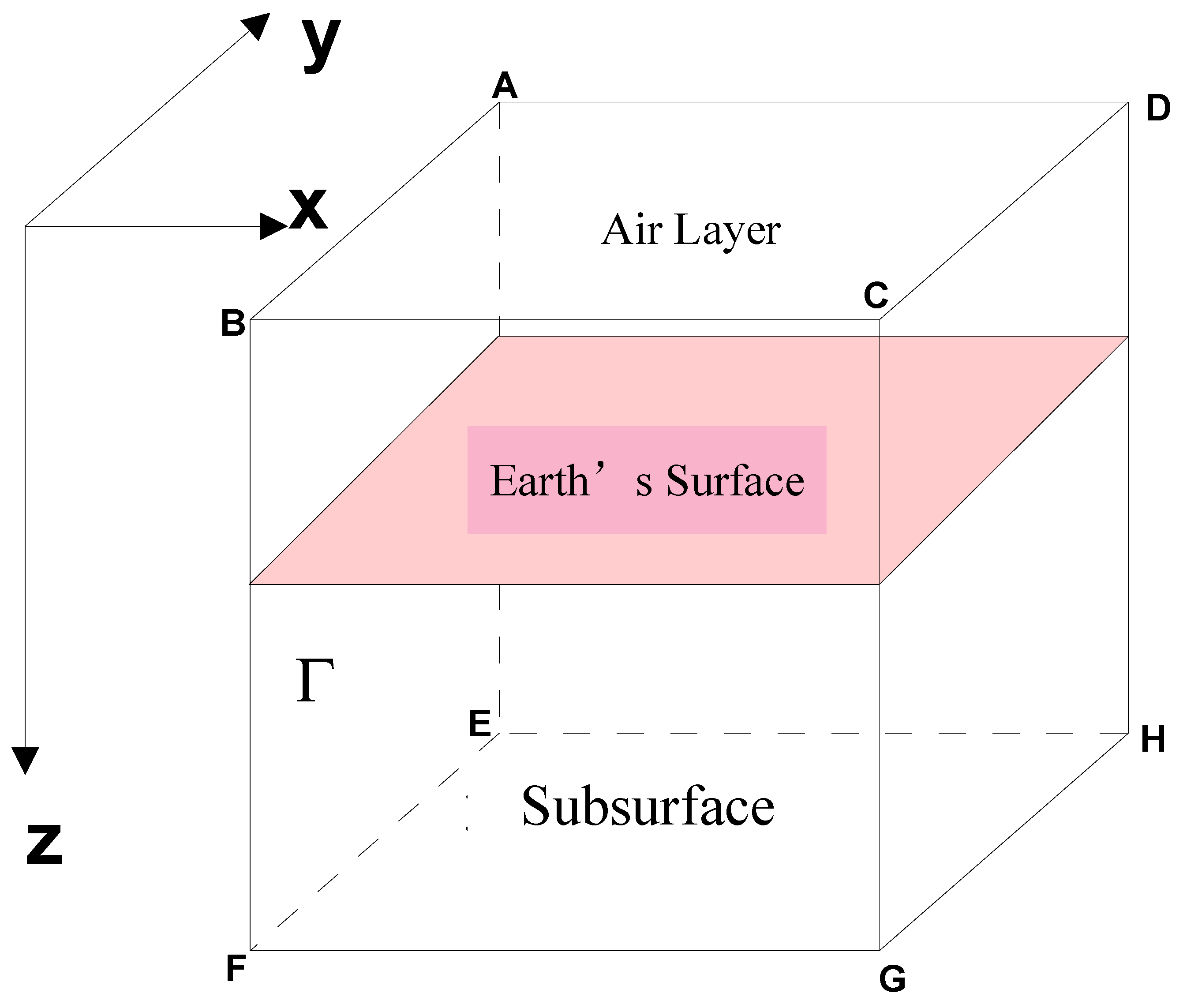
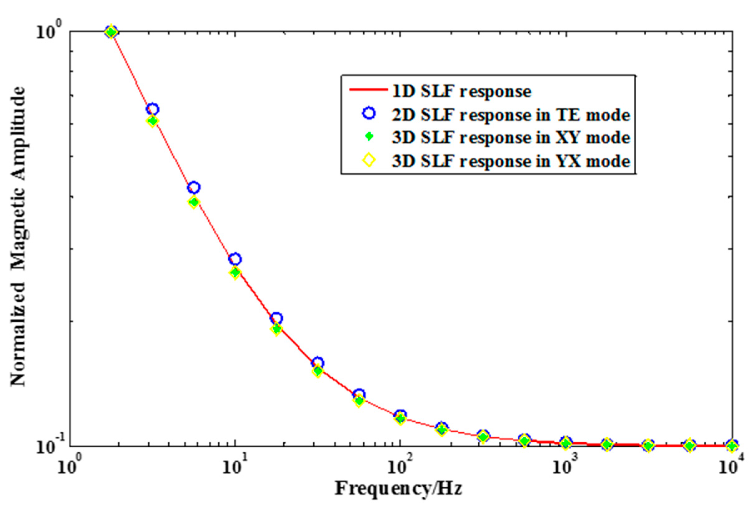
3.1. Finite Element Forward Modeling

The magnetic amplitude responses of 1-D, 2-D, and 3-D model assumptions should be obtained to guide geological exploration. For 3-D problems, the FEM calculation process starts from the electric field calculation with six lateral boundaries in a 3-D cube subdivision. The schematic diagram of the geological model is shown in Figure 1.
An orthogonal component of the initial incident plane wave field is distributed along the x-direction, and E x of the air layer in the model is set as 1 unit with other components as 0. As for the last four side boundaries, the direction of the electromagnetic field wave vector is perpendicular to the direction of the boundary normal. The infinitely deep bottom boundary condition is similar to that of the 2-D model, and the electromagnetic wave exponentially decays. The partial differential equations corresponding to the boundary value sets for the electric field components are listed below:
{ × ( × E ) k 2 E = 0 E x = 1 , E y = 0 , E z = 0 E × H Γ E x = c e k z , E y = 0 , E z = 0
where c is constant, k = i ω μ σ , and σ represents the uniform spatial conductivity at the bottom of the infinite depth.
Then, the variation of the function corresponding to the boundary value problem is also given:
{ F ( u ) = Ω × δ u × u d Ω Ω k 2 u δ u d Ω + E F G H k u δ u d Γ u | up = 1 δ F ( u ) = 0
where u   =   E x , k   =   i ω μ σ .
A simple 1-D model was designed to analyze the accuracy and computational efficiency of the algorithms. The designed four-layer model and forward modeling codes in the literature were still used. Furthermore, these algorithms were also evaluated using general 3-D geo-electrical models proposed by the Comparison of Modeling Methods for ElectroMagnetic Induction (COMMEMI) and adopted by academic communities [28]. We calculated the 1-D analytical solution of the magnetic amplitude response, the solution in the 2-D TE mode, and the 3-D numerical solution in the XY and YX modes. As the horizontal magnetic field component was a constant in the 2-D TM mode, only the magnetic amplitude response of the TE mode was calculated here. The 3-D model was divided into 32 × 24 × 28 grids, and the surface sites were all taken at the center of the surface. As shown in Figure 2, the 1-D, 2-D, and 3-D solutions of the normalized magnetic amplitude responses were coincident. Although the magnetic amplitude responses measured under actual conditions had random variations, normalization responses were stable, effectively eliminating the influence of random fluctuations. The 3-D modeling results showed that averagely normalized SLF magnetic amplitudes should be used in geological interpretation [28].

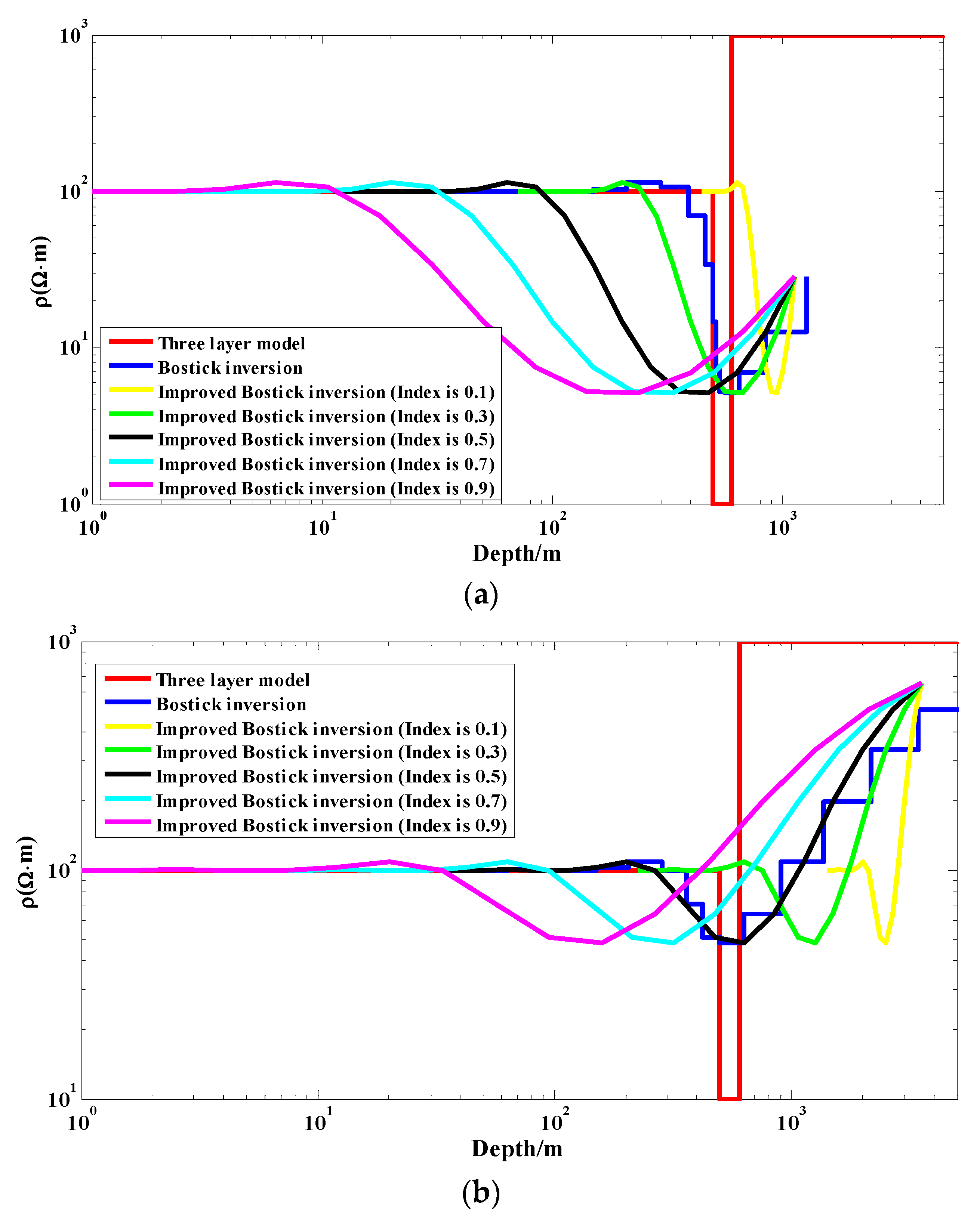
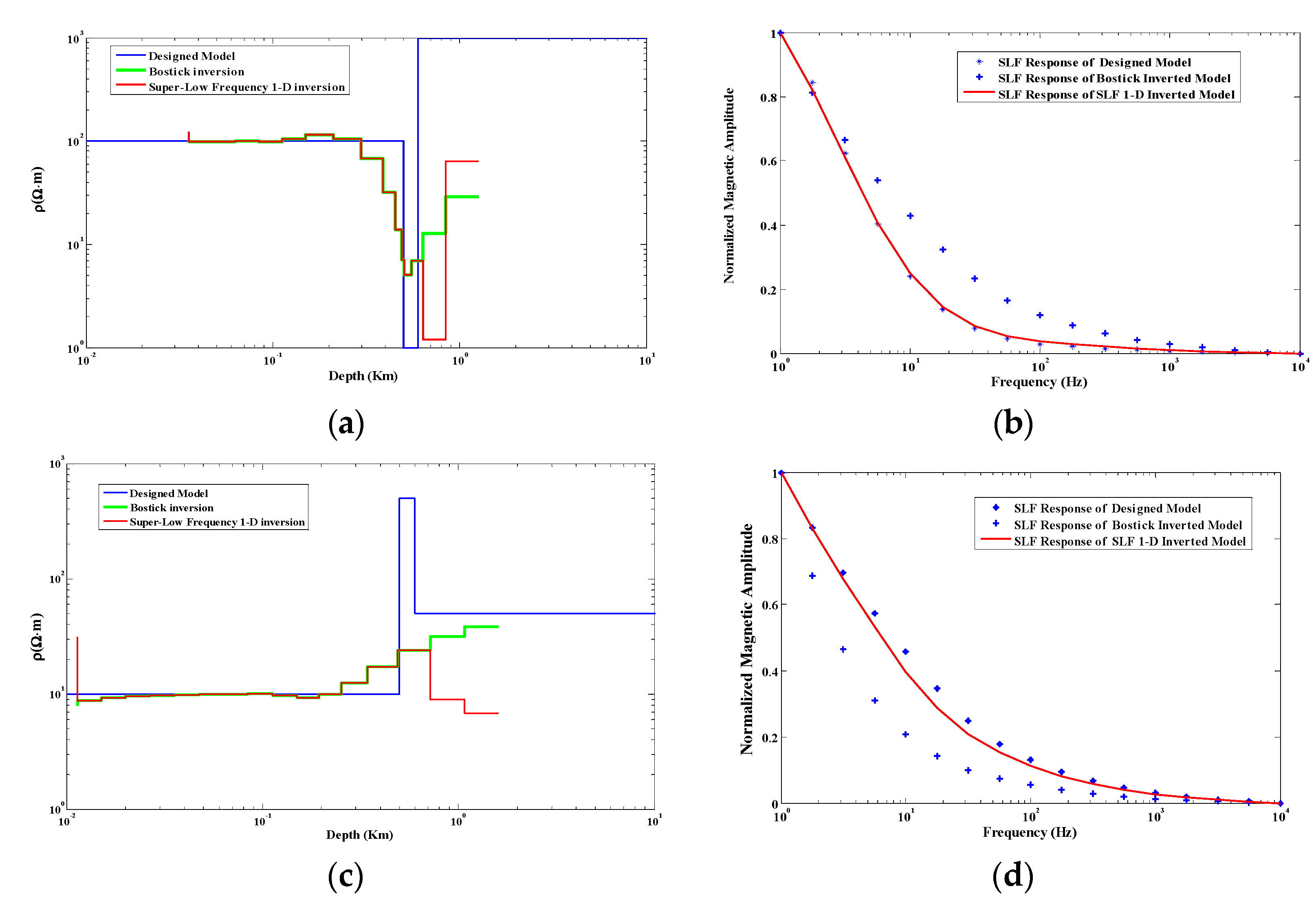
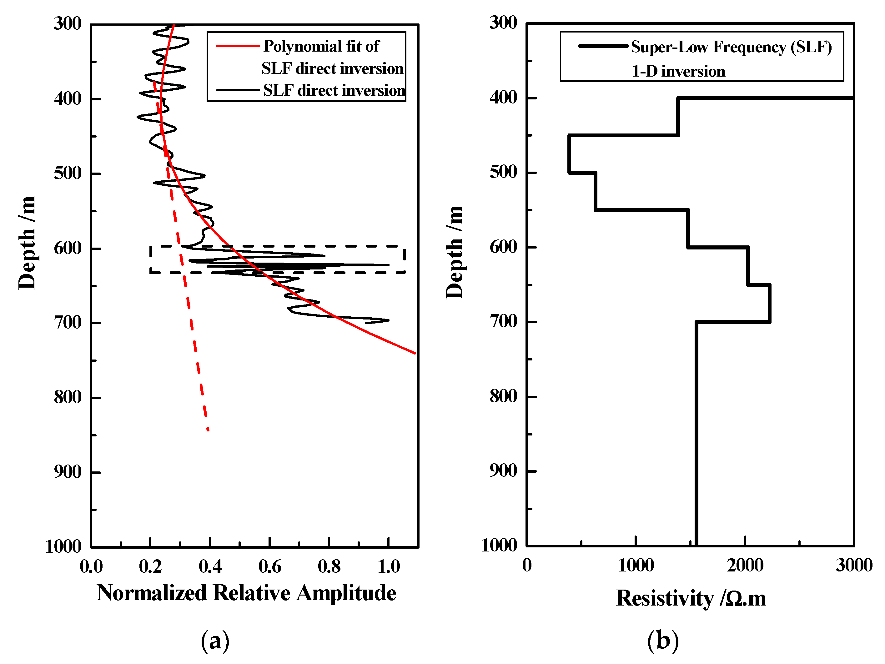
3.2. Direct Frequency-Depth Transformation

One of the critical problems using the SLF method in actual geological exploration is how to realize the frequency-depth transformation. The direct conversion of the frequency spectrum to the depth spectrum basically comes from two kinds of classical assumptions: one is Schmucker’s method, which calculates the depth information according to the relations among the impedance response, the resistivity, and phase [45]. However, this method is invalid when the target layer has low resistivity while the underlying strata are thick and have high resistivity. The other empirical transformation commonly used in the MT method is Bostick inversion, and the general form is:
ρ ( H ) = ρ a ( ω ) [ π 2 ϕ ( ω ) 1 ]
H = ρ a ( ω ) ω μ
where H is the inversion depth, ρ ( H ) is the inversion resistivity, μ is the permeability, ω is the angular frequency, ρ a ( ω ) and ϕ ( ω ) are the apparent resistivity and phase at an angular frequency, respectively. Equation (16) itself is very similar to the exploration depth Equation (17) for the homogeneous half-space model:
D = ρ ω μ
where D is exploration depth, ρ is uniform half-space resistivity, μ is permeability, and ω is the angular frequency. ρ a ( ω ) is the apparent resistivity at the intersection of two asymptotes at a specific frequency.
The asymptote intersection ρ a is the result of comprehensive resistivity ρ g , which should be a compromise between the resistivity of the target layer and the following layers. It is assumed that the target layer and the subsequent layers can be regarded as a homogeneous body, and its resistivity is set as the comprehensive resistivity ρ g , which replaces ρ a . The compromise resistivity chosen in this study seems to originate from the spatial correlation (also called the “volume effect” in the electromagnetic sounding). This weighting function is controlled by the distance, which can be measured by the change of the weight coefficient. Therefore, the exponential parameter (corresponding to the distance weight coefficient) of formula (17) can be dynamically selected. The improved frequency-depth transformation formula can reasonably adjust the exploration depth range and extract the layer thickness. In the SI system, the expression is
H = 356 ρ g f c
where H is the evaluated depth (m), ρ g is the general resistivity (Ω·m), f   is the frequency (Hz), and c is the adjusted index. This frequency-depth transformation formula based on inverse distance weighting is an interpolation method with the distance as the weight, representing the “volume effect” connotation.
A three-layer geo-electrical model was still selected here. The specific model contained a caprock (500 m thick, resistivity 100 Ω·m), an intermediate target layer (100 m thick, variable resistivity), the base is infinitely deep, and the resistivity is 1000 Ω·m. The improved Bostick inversion based on formula (18) and the classical Bostick inversion was used for the comparative analysis [28]. The semi-quantitative inversion named “improved Bostick inversion” is derived from the classical Bostick inversion and is further appropriate for the SLF method. The formula can be used by adjusting the general resistivity and index c according to the actual geological settings so that it is easy to use for the direct interpretation of target layers. When the middle layer is 1 Ω·m, the comprehensive resistivity is the compromise resistivity of the middle layer and the bottom plate 10 Ω·m. The exponent parameter c is 0.1 to 0.9, respectively, and the improved Bostick inversion results can be obtained.
A comparison of the original model and Bostick inversion results is shown in Figure 3a. When the parameter is 0.1, although the layer identification accuracy is high, the exploration range is limited and deviates from the exploration target layer; when the parameter is 0.3, the depth and thickness of the target layer of the improved Bostick inversion are basically consistent with the Bostick inversion results, but the accuracy is not as high as that of the parameter 0.1. Although the reservoir can be roughly identified when the parameter is set to 0.5, the identification accuracy is lower than the inversion result of “c = 0.3”. Therefore, the index parameter of the improved frequency depth transformation can be a number between 0.1 and 0.3 to ensure that the improved Bostick formula with a satisfactory exploration depth range and the target layer identification accuracy at the same time. Additionally, when the intermediate layer is 10 Ω·m, the parameter c is set from 0.1 to 0.9, respectively, as shown in Figure 3b. When the parameter is 0.1 and 0.3, the accuracy is high, but the depth range is narrow, deviating from the exploration target. When the parameter is 0.5, the results are almost the same as that of the Bostick inversion, but increasing the exploration depth range often reduces layer identification accuracy. However, the ideal accuracy cannot be given when the index parameter is larger than 0.5. Therefore, the exponent parameter of the final formula (18) can use values between 0.1 and 0.5.
The c index is the adjustable index of the frequency term. The formula could be reasonably adjusted through trial-and-error tests and is suitable for the objective exploration depth and the estimation of the layer thickness in practice. The final semi-quantitative formula is in accordance with well log data with high accuracy. Furthermore, a nonlinear inversion analysis was also comparatively required in the next section for a further inversion accuracy evaluation.

3.3. Nonlinear Regularization Inversion Algorithms

The nonlinear inversion of the normalized magnetic amplitude response is a process of optimally estimating the subsurface resistivity information by fitting the forward modeling responses through a nonlinear regularization calculation. The constraint inversion algorithm based on the prior model introduces the idea of Tikhonov regularization [50,52]. We assume that d   is the measured data vector, m is a model parameter vector, and F is the forward process from the model to data. Then, the overall objective function of the inversion problem is:
ϕ ( m ) = | | W d [ d F ( m ) ] | | 2 + α | | W d [ m m 0 ] | | 2
where ϕ ( m ) is the objective function; α   is the regularized parameter; W d is the observed data weight coefficient matrix; W m is the model weight coefficient matrix, and m 0 is the prior model. F ( m )   is expanded by Taylor’s formula. Ignoring the quadratic term, we have:
ϕ ( m k + 1 ) = | | W d [ d ( d k + j k Δ m ) ] | | 2 + α | | W m [ m k m 0 ] | | 2
where m k is the k iterative value of the model, and d k = F ( m k ) is the model correction amount Δ m = m k + 1 m k , and J k is the sensitivity matrix. We differentiate the above objective function with respect to Δ m and set it to 0. Write it in the iterative form:
m k + 1 = m k + Δ m = m k + [ ( J k ) T W d T W d J k + α W m T W m ] 1 [ ( J k ) T W d T W d ( d d k ) + α W m T W m ( m 0 m k ) ]
Equation (21) is an iterative form of the 1-D regularization inversion based on the prior model by solving   Δ m to obtain a new model parameter vector. This step is iteratively repeated until the set threshold ϕ ( m ) is met. A uniform half-space can be chosen as the prior model during the inversion process. If there are simultaneous MT data, the Bostick inversion results can be obtained as a priori model, and more reasonable results can be obtained.
A three-layer model is also designed to verify the inversion algorithm. The first low-resistivity target layer model includes a cap layer (500 m thick with a resistivity of 100 Ω·m), an intermediate target layer (100 m thick with a resistivity of 1 Ω·m), and an infinitely deep base with a resistivity of 100–1000 Ω·m. The 1-D inversion takes the Bostick inversion result as the initial prior model, and the final RMS is 0.81 in ten iteration steps. The comparison of the 1-D inversion results and Bostick inversion results are shown in Figure 4a. The 1-D inversion not only achieved the accuracy level of the Bostick inversion but is also closer to the true value of the low-resistivity anomaly. In addition, the magnetic component response of the inversion model is calculated, and as shown in Figure 4b, is compared with the forward responses. The response of the 1-D inversion model is closer to the actual response. In contrast, the second model includes the cap layer (500 m thick, resistivity 10 Ω·m), the middle target layer (100 m thick, resistivity 500 Ω·m), the base is infinitely deep, and the resistivity is 50 Ω·m. The inversion process is the same as that of the above low-resistivity target model, and the results are shown in Figure 4c. Compared with the Bostick inversion results, the 1-D inversion of the SLF method can better highlight high-resistivity anomalies with improved identification ability. In addition, compared with the response of the original model, as shown in Figure 4d, the 1-D inversion response of the SLF method is closer to the actual response, which is much better than that of the Bostick inversion of the AMT method. The above two examples demonstrate that the 1-D inversion of the normalized magnetic amplitude response can also extract the subsurface electrical information, and the inversion accuracy reaches or even exceeds the classical Bostick inversion accuracy. The inversion time of the SLF is much less than that of the AMT inversion. In the future, more 2-D and 3-D inversion algorithms of the SLF method should be proposed to further explore the capability of the subsurface interpretation.

4. Magnetic Component Detection and Data Processing

The SLF method mainly uses magnetic sensors to collect the time-series signal. For magnetic sensors, high sensitivity, wide frequency band, and large dynamic range should be guaranteed, and repeatability testing and instrument calibration are also required. There mainly contains multiple superpositions, notch filtering, and spectrum analysis algorithms for data preprocessing. Moreover, the independent component analysis, wavelet analysis, and empirical mode decomposition methods are also introduced [43]. These methods have widely been used in geological structures, water-rich areas, geothermal reservoirs, and other fields, achieving excellent results [53,54,55].

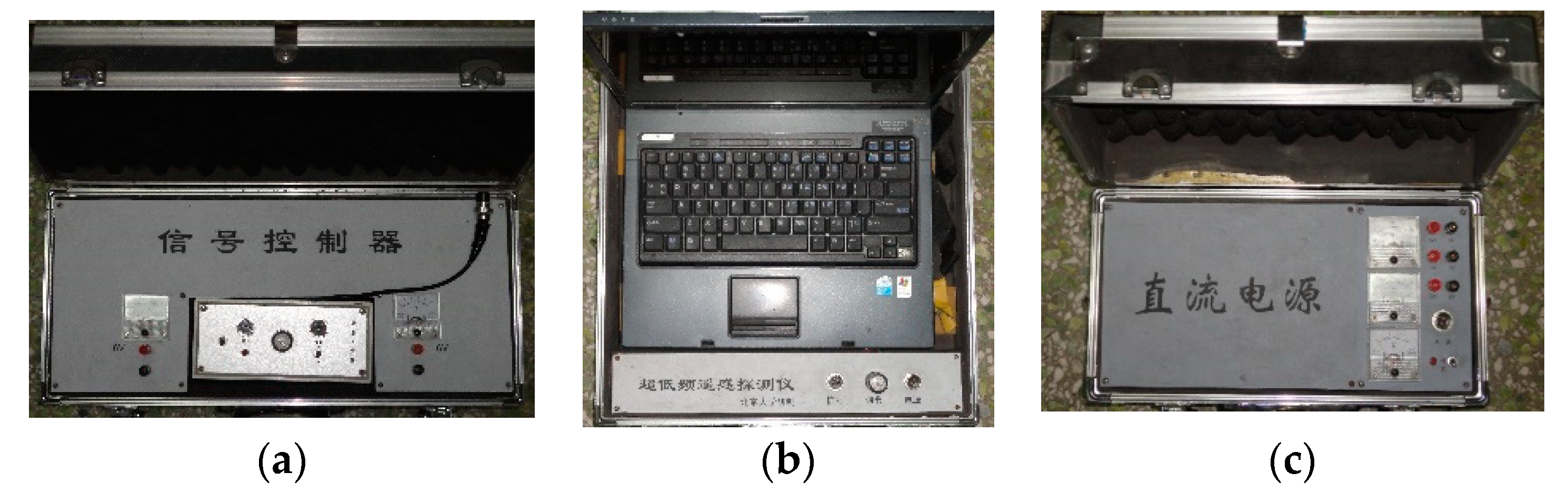
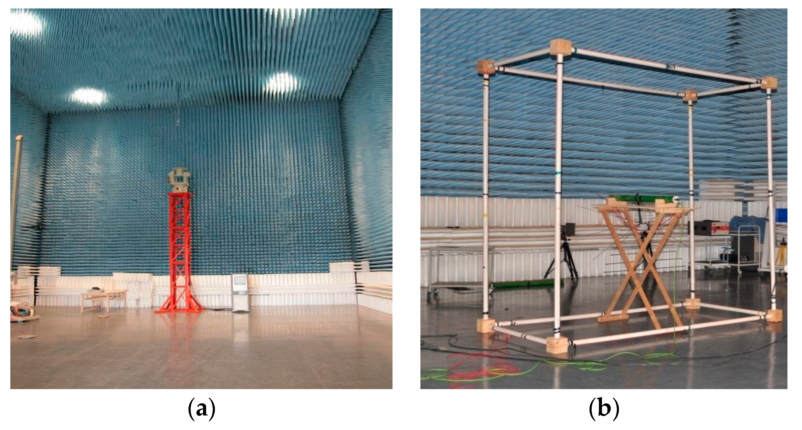
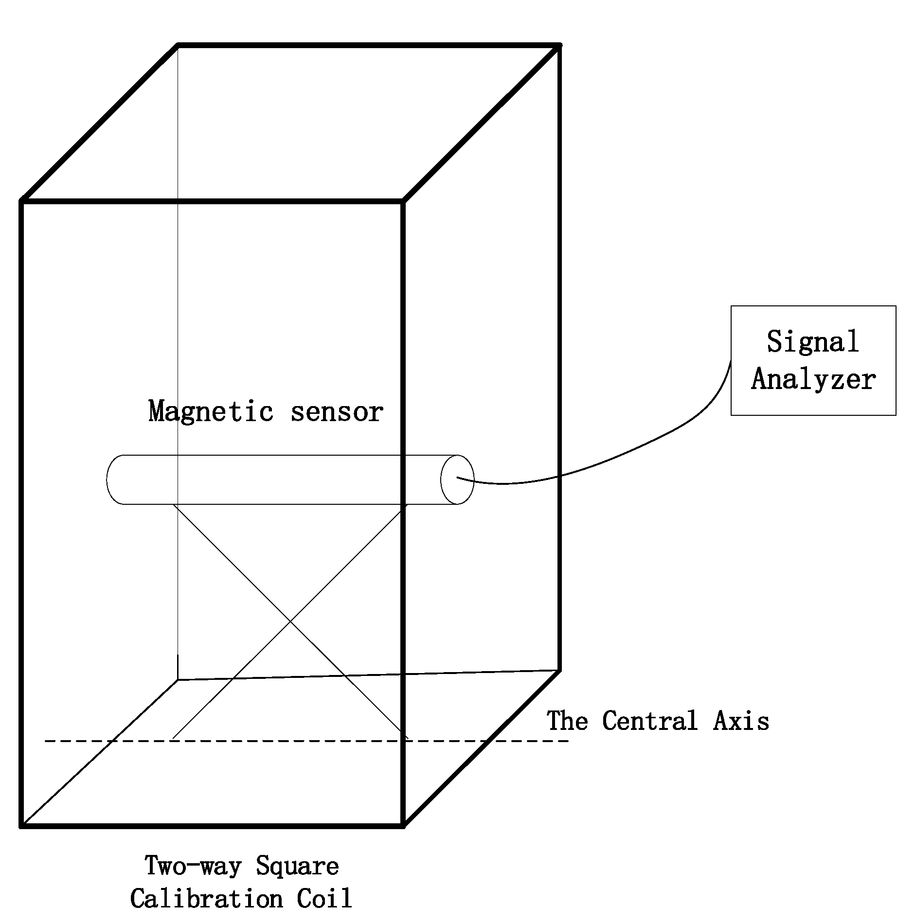
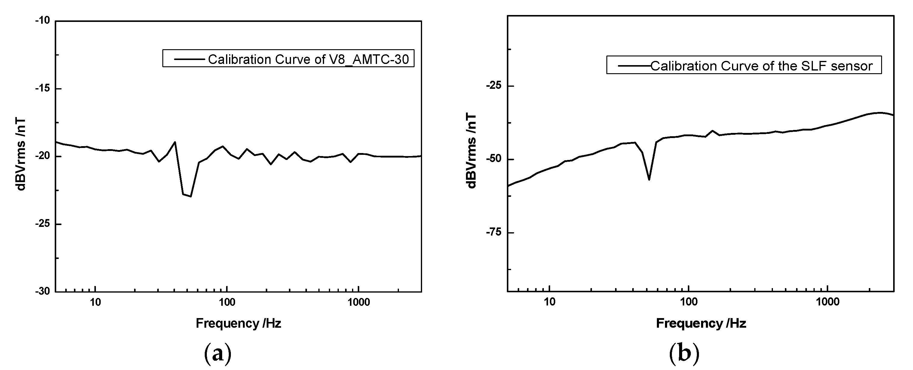
4.1. BD-6 Magnetic Sensor and Its Calibration

High-quality data detection is significant for improving signal resolution and inversion accuracy. The BD-6 electromagnetic detector developed by the authors is mainly used [56], and the V8-AMT module from Phoenix Canada is also comparatively utilized. The V8-AMT module mainly contains the host, power supply, magnetic track, and electric channel. Using the five-component electromagnetic channel ( E x , E y , H x , H y and H z ) detection method, the audio electromagnetic signal in the range of 1–10000 Hz is collected with high precision. In contrast, the BD-6 electromagnetic detector receives the 3–3000 Hz magnetic component signal, consisting of a high-precision magnetic sensor, a host, and a power supply, as shown in Figure 5. The magnetic sensor includes modules such as the magnetic rod, wiring, amplifier circuit, program-controlled trap circuit, and interface high-speed acquisition circuit. The minimum received induced voltage value is 0.1 μV, and the magnetic response can be sensitively obtained. The sensor noise is minimal, and the output gain of the preamplifier can amplify the weak signal at the microvolt level by 106 times. The host includes the data acquisition, format conversion, storage, and control units and can realize the hardware notch of power frequency (50 Hz) harmonics with a portable power supply. The whole set of equipment has advantages such as low noise, portability, and high detection efficiency. A geological survey usually has an average cost of hundreds of dollars with more measurement sites. Therefore, the SLF method has a higher cost-performance ratio than other conventional electromagnetic methods.
The magnetic sensor should be calibrated to evaluate the electromagnetic signal reasonably, and a magnetic shielding room is utilized, as shown in Figure 6. The calibration coil adopts a square Helmholtz coil, consisting of two coaxial square coils of the same size. According to the magnetic field calculation formula, if the distance between the two coils is half of the square length, a magnetic field is uniformly generated at the center of the coil. By adjusting the current flowing in the coil, the strength of the magnetic field at the axis position is changed with a calibration signal generated.
The magnetic sensor calibration test requires an amplitude-frequency calibration in the Super-Low Frequency (3–3000 Hz). The test diagram is shown in Figure 7 below.
The calibration results of the sensor are compared with those of the V8-AMT high-precision magnetic sensor, Phoenix Company, Canada, as shown in Figure 8a,b. Despite the notch filtering of the 50 Hz power frequency interference, the amplitude-frequency curve of the magnetic sensor still has a relatively flat characteristic in the Super-Low Frequency band (3–3000 Hz). Additionally, the calibration curves of the two magnetic sensors still have an order of magnitude difference in amplitude which is mainly caused by the two amplifying circuits and internal correction circuits. The absolute magnetic component response quantity can be directly obtained so that there is no essential difference in use. Therefore, the calibration curve of the sensor fully meets the requirements of the data detection accuracy.

4.2. Magnetic Component Signal Processing

Spectral estimation is mainly intended to suppress noise and improve the effective response. It is usually assumed that the signal or noise follows a Gaussian distribution, and then the second-order statistics are calculated to complete the spectral estimation [57,58]. However, for natural source electromagnetic signals, the non-Gaussian features are obvious. When the received magnetic component signal includes a non-Gaussian signal and a Gaussian noise independent of each other, the overall signal has higher-order statistical features [59]. Signal analysis methods based on higher-order statistics contribute to the non-Gaussian signal estimation. The empirical mode decomposition method (EMD) is introduced and appropriately applied to magnetic component processing. The calculation steps cover the signal input, adaptive extraction of eigenmode functions (IMFs), and signal decomposition [27,60]. The experiment showed the simulated signal analysis using 50 Hz power frequency noise and a random magnetic signal.
Signal = 10 × sin ( 100 π t ) + r a n d ( 1 , n )
First, the Fourier transform was used to extract the spectrum curve of the simulated signal, and then the EMD method was performed on the spectrum signal, as shown in Figure 9. The first four eigenmode functions included 50 Hz power frequency interference noise, while the last four eigenmode components seemed almost unaffected by the noise. Therefore, the first four disturbed eigenmode components were superimposed, and the last four were superimposed. The results shown in Figure 10 demonstrated that the spectrum of the random signal was recovered with 50 Hz power frequency interference compressed.
An actual SLF curve obtained at the CBM enrichment area, Qinshui Basin, was taken as an example for illustration, as shown in Figure 11a. The raw curve was observed in September 2011 near the Well 1-4 (see details in Section 5.1). The two arrows from top to bottom show the location of two 50 Hz power frequency harmonic interferences. First, the curve was empirically decomposed using the EMD method, and seven intrinsic mode functions (iIMFs) could be obtained adaptively, as shown in Figure 11b–h. The black arrows in these IMFs in the figure represent the decomposed 50 Hz harmonic interference components, indicating that the third to sixth IMFs were components polluted by power frequency noise. The first and second IMF components showed high-frequency information far beyond the 50 Hz harmonic interference, which could be regarded as valuable signals. The last IMF component was presumed to be a gently varying background field. Then, the curve could be reconstructed by setting the noise-polluted components’ weight coefficient to zero and superimposing other non-noise components, as shown in Figure 12b. Compared with the original acquisition curve in Figure 12a, the two 50 Hz power frequency harmonic interferences indicated by the black arrows were removed. However, some high-frequency random interference still existed in the reconstructed signal. By using the wavelet analysis method and the multi-scale filtering, high-frequency random noise was almost filtered out. A three-layer “DB4” wavelet was used to decompose the reconstructed curve, and the high-frequency detail part was set to the denoising threshold and then reconstructed to obtain the magnetic amplitude curve, as shown in Figure 12c. As indicated by the black oval, the effective signal was further highlighted, and the effect of high-frequency random noise was reduced. In practical applications, data processing methods suitable for this kind of non-stationary SLF signals are also developed in the adaptation of the BD-6 system. The ultimately processed SLF curve is ready for geological interpretation of objective layers in a geological survey. This has depicted that the SLF method has gradually grown as a new potential electromagnetic sounding tool compared with the classical AMT method.

5. CBM Reservoir Interpretation in Qinshui Basin

5.1. Study Area and Field Experiments

Qinshui Basin is located in the southeast of Shanxi Province in Figure 13. It is a late Paleozoic residual basin formed by the Indosinian movement, especially the Yanshan movement [1,61]. Carboniferous-Permian coal-bearing sediments are widely distributed in the area, and the main CBM enrichment areas spread in the Late Paleozoic Taiyuan Formation and Shanxi Formation in the south. As shown in Figure 13, the western boundary is the closed Sitou fault. This fault makes a tremendous difference in the gas content between its two sides. The east and south are hydrodynamic sealing boundaries delineating gas reservoirs that belong to different flow units.
The study area is located in the Hudi block south of the Qinshui Basin, as shown by the red five-pointed star on the left in Figure 14. The local tectonic direction in the area is almost the same as the regional tectonic direction. The general strike is NNE or nearly north-south, and the dip is NWW, with the dip angle less than 10°. From southeast to northwest, Ordovician, Carboniferous, and Permian are gently exposed in turn. The Quaternary is widely covered on the abovementioned strata, with a total thickness of nearly 32 m. The main hydraulic recharge areas of CBM reservoirs are enclosed by the southeast, northeast, and northwest boundaries (see the arrows). The lowest water level is along Yangcheng and Qinshui. Groundwater in the shallow layer near Zaoyuan in the north watershed runs off to the south and forms a hydrodynamic seal. The Taiyuan Formation outcrop with a hydraulic conservancy (shown by the underground waterline and their flow directions) also contributes greatly to the CBM accumulation. Additionally, the faults in favor of the uneven distribution of coalbed methane (CBM) reservoirs’ have been provided. These references all account for the “gas content” map. The distribution of the No. 3 reservoir in this area is shown on the right side of Figure 14, and the spatial CBM distribution is uneven. According to the CBM accumulation model in this area, other surrounding rock layers may have fissure water enrichment except for the mudstone aquifer. In particular, the reservoirs are often overlaid with stable aquifers and, therefore, significantly exhibit low resistivity, which can be used as target layers for the SLF interpretation.

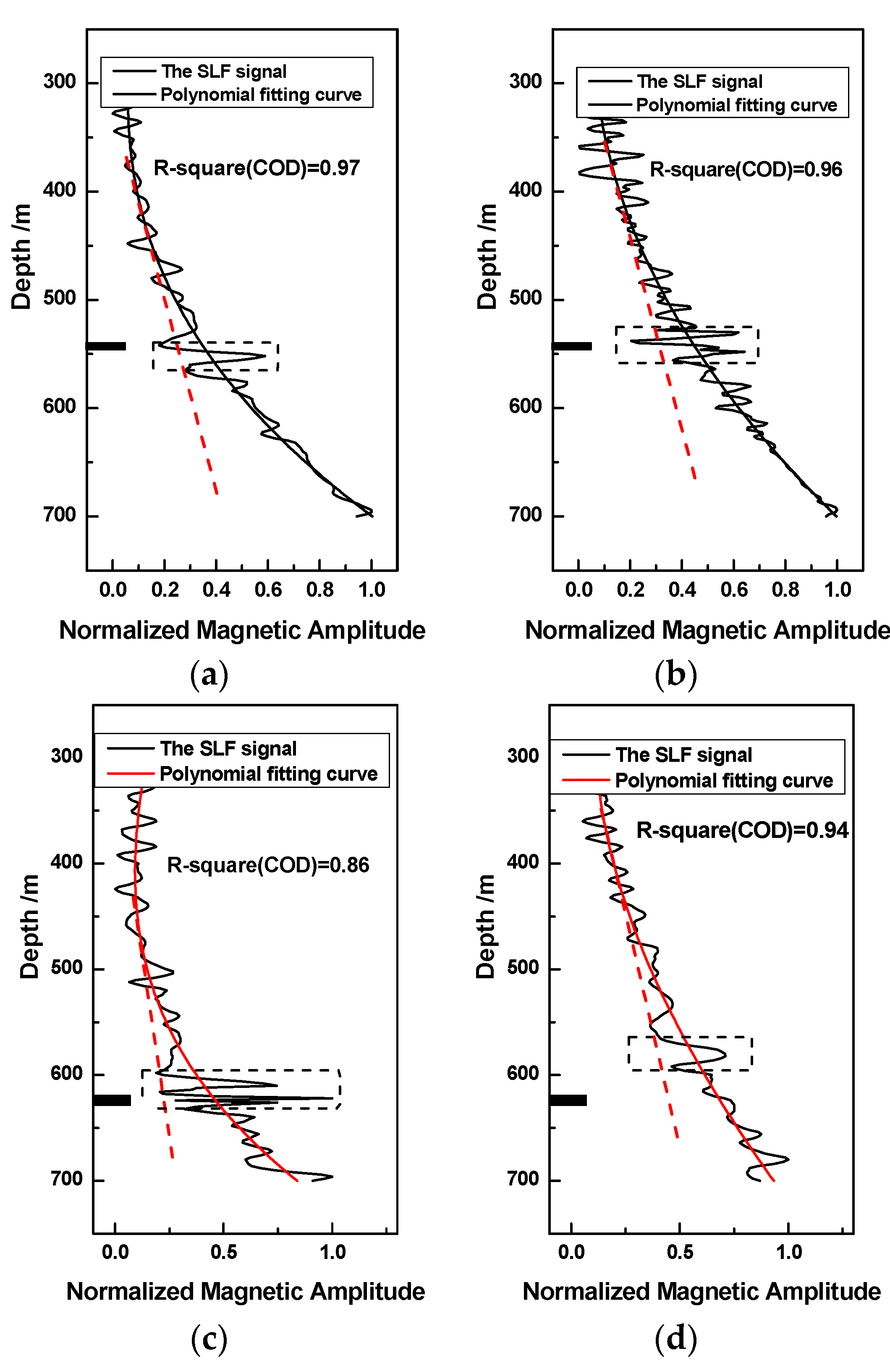
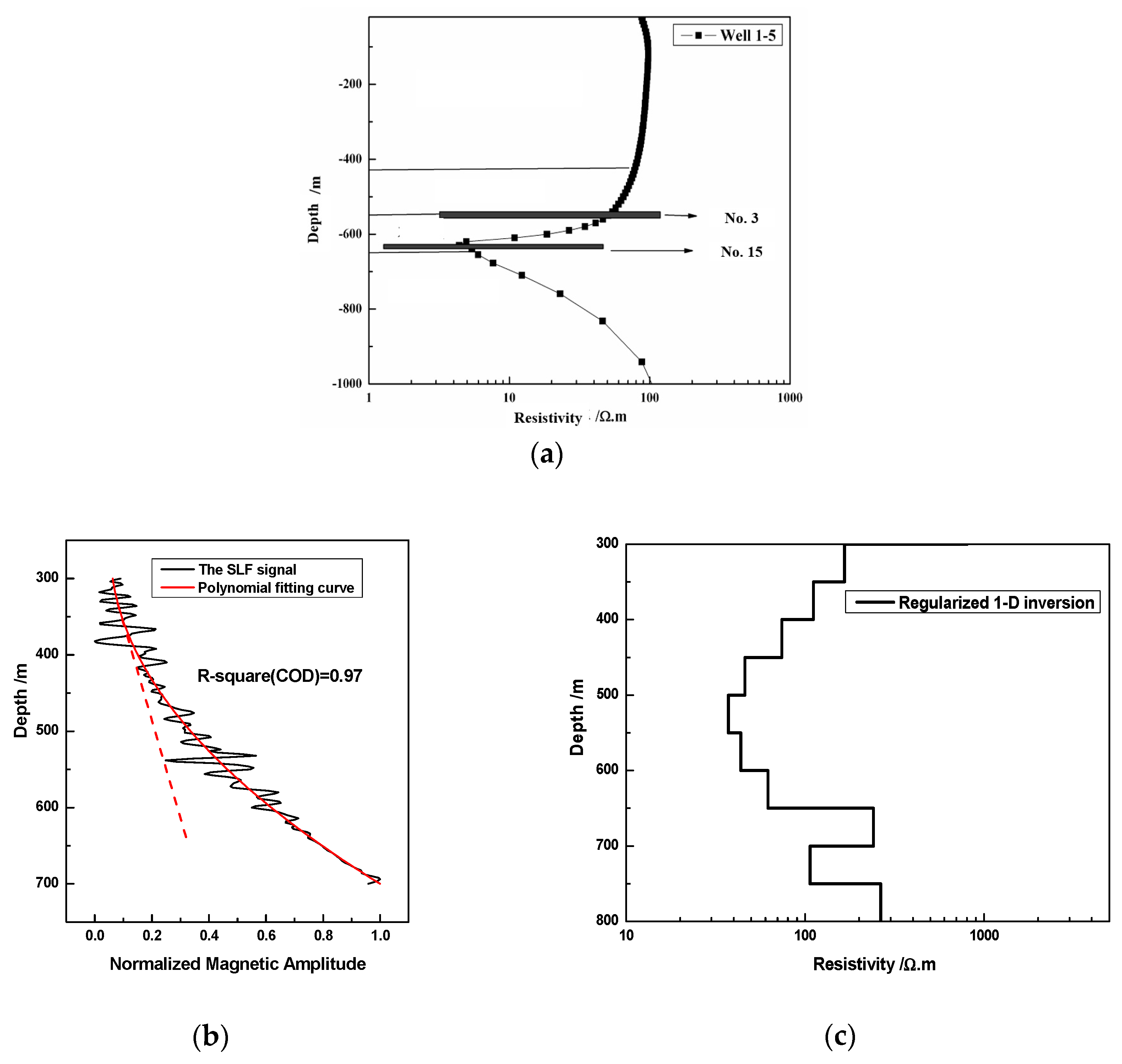
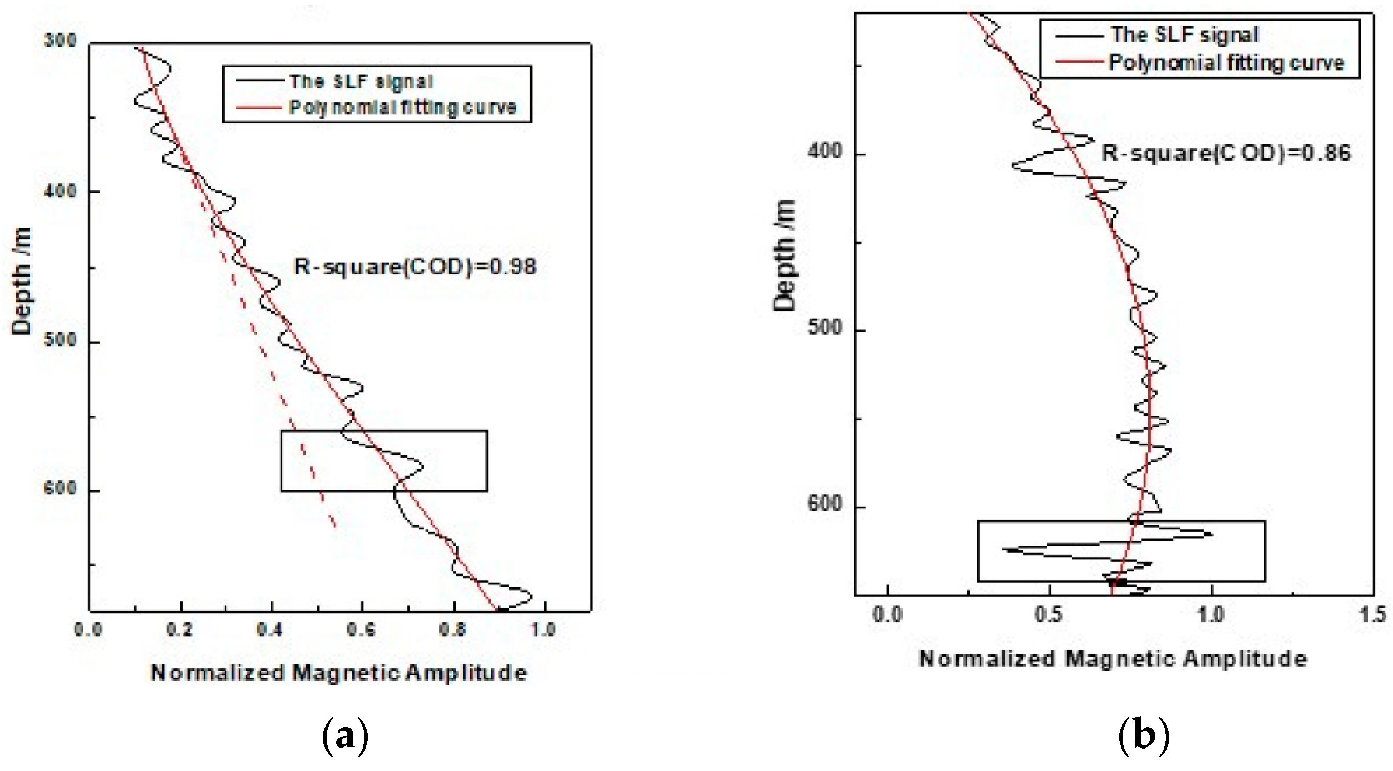
5.2. Reservoir Interpretation Based on Low-Resistivity Features

The in-situ identification of reservoir distribution usually mainly uses seismic attributes, AVO anomalies, and elastic impedance characteristics and establishes an empirical coupling relationship with coal reservoirs [62,63]. However, there is no convincing explanation mechanism [64]. In contrast, electromagnetic exploration is worthy of further study. The groundwater salinity of the reservoirs is 800–2400 mg/L, and the aquifer has low resistivity. The drilling data shows that the resistivity of the aquifer is lower than 50 Ω·m, and the non-aquifer is basically between 200–1000 Ω·m. The high-resistivity base is above 3000 Ω·m. The previous theoretical analysis has suggested that the SLF responses of reservoirs are more sensitive to the low-resistivity layers in favor of the feasibility of directly extracting the low-resistivity reservoirs first [65]. According to the field survey, the CBM wells in the study area extract a large amount of groundwater for drainage and pressure reduction to facilitate the CBM desorption and escape. The reservoirs may have a large amount of groundwater due to their connection with the roof and floor aquifers, which is inferred that the thickness of the entire aquifer is 100–200 m. Therefore, the SLF method can be used to predict the sensitivity of water-bearing low-resistivity layers, and the location of reservoirs can be indirectly identified.
The SLF field experiments around Well 1-4 were carried out in May 2010 and Well 1-5 in August 2011. The BD-6 detector was located 30 m away from the drainage well and far from various power lines. The magnification of the front and rear of the system was three times, and five sets of data were collected with the sensor rotated every 90°. The results were processed using the average normalization, filter denoising, and frequency-depth spectral conversion described in Section 4.2. The comprehensive resistivity used in the frequency-depth spectrum conversion formula was 400 Ω·m, and the exponent parameter was 0.5 [28]. Finally, the depth spectrum interpretation curve was obtained by this direct inversion. In addition, the 1-D inversion calculation was also carried out by using the developed nonlinear regularization algorithm in Section 3.3, and the 1-D resistivity profiles of the two wells were given. As shown in Figure 15a, the interpretation curve of Well 1-4 by the SLF method after the frequency-depth transformation was given. The results deduced that the inflection point was approximately 400 m deep. The curve was warped to the right relative to the trend line, indicating the existence of a low-resistivity layer. Due to the limitation of the exploration range, there is a possibility of the existence of low-resistivity layers at least deeper than 600 m. Then, 1-D optimization inversion was performed with the prior model set as a uniform half-space model of 100 Ω·m. The inversion was iterated 30 times, and finally, the 1-D regularized inversion profile was obtained by convergence, as shown in Figure 15b. In contrast, the 1-D optimization inversion results showed that a low-resistivity layer distributed from 400 m to about 620 m, indicating that the distribution range of low-resistivity bodies was very wide, with the resistivity lower than 100 Ω·m. The next step was to enter the high-resistivity layer. According to the field survey, the reservoir was in continuous groundwater drainage, indicating that the reservoir itself was also gradually filled with groundwater. Additionally, the underlying reservoir was also possibly low resistive due to the hydraulic communication with the hydraulically filled caprock. The SLF method’s inversion results illustrate the distribution of low-resistivity layers covering the caprock, floor limestone aquifer, and reservoir. This was consistent with the analysis results of the on-site production status.
Well 1-5 is located 100–200 m to the east of Well 1-4. The geological data shown in Figure 14 reveals that an F1 fault exists between the two wells. This fault leads to the overall decline of the water-bearing overburden, which may also lead to the hydraulic connection between the drainage reservoir, the cap roof, and the bed floor, forming a huge thick and high-conductivity layer. According to the drilling data of Well 1-4, No. 15 coal seam is 543–546 m. The No. 15 reservoir of Well 1-5, observed at 618–621 m, is 80 m deeper than Well 1-4. This indicates that the fault displacement is about 70 m–80 m. As shown in Figure 16a, the direct depth transformation results showed that a low stop band appeared from 450 m, about 50 m deeper than Well 1-4. The reservoir location is about 590–630 m, and it could basically be deduced that the fault throw might be about 50 m, which is almost consistent with the actual depth distance. By contrast, the 1-D optimized inversion curve in 16b showed a low-resistivity layer starting from 450 m to 600 m deep, with a resistivity less than 500 Ω·m. It was inferred that the low-resistivity layer had a low water content, and on the other hand, there might be no hydraulic connection between the reservoir and its roof floor. This factor could also be seen from the direct depth transformation results of the two wells. Compared with the trend line in the response curves of Well 1-5, the upward deviation was smaller than that of Well 1-4, indicating that its resistivity was higher than that of the water-rich layer in Well 1-4. According to the production status of the two wells, the gas production rate of Well 1-4 was slower than Well 1-5. As is known to all, the hydraulic connection with the fault may harm the CBM production, and therefore the production loss of Well 1-4 should be due to the adjacent fault.
The experiments demonstrate that the SLF method can qualitatively identify the low-resistivity distribution and quantitatively invert the resistivity profile, especially low-resistivity features. As for the target layer, whose buried depth is 500–700 m, the preliminary results show that the magnetic component inversion can realize the low resistive target layer identification accuracy of approximately 100 m.

5.3. Reservoir Identification Using Electromagnetic Radiation Anomalies

The feasibility of extracting electromagnetic radiation (EMR) anomalies from ground measured data to evaluate underground media has been verified by field experiments [14,15,66]. The previous theoretical analysis shows that the EMR signal can be extracted from reservoirs as an abnormal signal in this background field [43]. A high-amplitude anomaly in the upturned section is found from the processed results of measuring sites near Well 1-5 in Figure 16a,b. With the related noise interference eliminated, it is inferred that it comes from the low-frequency EMR signals generated during the drainage process. According to previous research, servo pressurization in various types of coal and rock could generate electromagnetic radiation. The higher the reservoir pressure, the stronger the radiation signal. The frequency range is mainly concentrated in the low-frequency [67,68,69]. In particular, the low-frequency (100 kHz–1 Hz) radiation signal has rich frequency features and strong signal amplitudes [66]. Even in the case of the coexistence of gas and water, the coal rock with flowing gas inside generates EMR signals excited in the form of electromagnetic pulses. When the received pulses are superimposed together, local wave packets will form so that they can be used to judge the CBM production status with the frequency-depth transformation [15]. If the EMR intensity at the corresponding depth is high, it can be extracted and used to identify the reservoir distribution. Figure 17a showed that this radiation anomaly was also just below the aquifer cap, with inferred depths ranging from 540 m to 550 m. The drilling data of Well 1-4 revealed that the No. 15 coal reservoir was located between 545 m and 551 m, and the No. 15 coal reservoir was in the production status. Therefore, the results inferred based on the EMR anomalies of the reservoirs they were consistent with the actual production. Figure 17b shows the response curve observed one year later. The reservoir depth did not change much based on the EMR anomaly extraction, which indicated that Well 1-4 had relatively stable drainage and production.
For Well 1-5, the August 2011 results showed a corner point from 510 m, about 30 m deeper than Well 1-4, as shown in Figure 17c,d. Combined with the on-site production status investigation of the two wells in August 2011, the drainage and production rate of Well 1-4 was significantly slower than that of Well 1-5. It was deduced that the No. 15 reservoir in Well 1-4 had a large water content, which reduced the gas production and water drainage. The production rate slowed down and gradually entered a period of productivity decline. In contrast, the No. 15 reservoirs in Well 1-5 had a lower water content, a larger gas production, and faster drainage and production. This could also be inferred from the fact that the reservoir produced a stronger EMR signal (higher amplitude anomalies circled by dashed boxes). However, the results of Well 1-5 in June 2012 showed a deviation of nearly 20 m in the explained reservoir depth compared with that in 2011, and the anomalous EMR intensity decreased. This was verified by the production history that the overlying surrounding rock was affected by the mining, and the mining rate decreased. The detection test also preliminarily showed that the SLF method had certain feasibility in identifying the drainage and production reservoir and monitoring the production status of CBM reservoirs.
In CBM reservoir exploration, the multi-solution problem would often be encountered. Through the joint electromagnetic detection comparison test, the generation of multi-solution can be reduced as much as possible. Therefore, the 3-D inversion of the AMT method was simultaneously carried out in the comparison test at the same measuring point of Well 1-5. According to the borehole data of Well 1-5, as shown in Figure 18a, it is revealed that the No. 3 coal reservoir is between 531 m and 536 m, while the No. 15 coal reservoir is between 618 m and 621 m, and the No. 15 coal reservoir is in production. One inversion curve from the resistivity profile given by AMT 3-D inversion can describe the distribution of low resistivity zones and indirectly infer the general distribution of CBM reservoirs reasonably. In contrast, the 1-D inversion of the SLF method can jointly detect and verify the conductive distribution of reservoirs and surrounding rocks in Figure 18c. The direction inversion with the EMR anomalies extraction in Figure 18b can provide more details on the production status of Well 1-5 [43].
In this process, the SLF method has the advantages of faster inversion and a more directly perceived interpretation than the AMT method. The two electromagnetic methods can cooperate to realize the reliable interpretation of CBM reservoirs.
In the field exploration process, it is usual to judge whether or not geo objects’ conductive images are illustrated using types of resistivity inversion algorithms of the SLF method or other electromagnetic methods. However, the existence of coal reservoirs cannot be directly determined. The problem encountered by these methods is that no reasonable coupling relationship exists between electromagnetic responses and reservoir parameters. Therefore, EMR anomalies extracted may be one of the best responses, which can better help judge the existence of coal reservoirs. The distribution of radiation anomalies can provide a reference for reservoir depth identification. At present, the anomaly depth ranges of wells are empirically extracted through visual interpretation compared to the actual reservoir distributions. The concept of reservoir identification resolution was proposed and estimated by the ratio of the depth to the thickness of the target layer, but this was not suitable for evaluating reservoir interpretation accuracy. This study proposes two parameters for the interpretation accuracy evaluation: reservoir interpretation depth deviation and relative deviation σ.
σ = H RE H SLF H RE × 100 %
where H RE represents the intermediate depth of the actual reservoir, and H SLF represents the SLF method estimate of the reservoir depth.
A series of field surveys using the SLF method have been carried out in the study area in the past years, and more logging data or production history have been used to verify the reservoir detection. In Figure 19, the data from the vicinity of Well 1-8 were collected in 2011 and 2012, respectively. EMR anomalies near the buried depth of the target layers are extracted. Most of the interpretation accuracy results are shown in Table 1. The results preliminarily support the feasibility of reservoir delineation based on EMR anomalies. In comparison, the absolute resolution capability using other electromagnetic methods for identifying reservoirs shallower than 1 km may be over one hundred meters. Of course, it is worth noting that EMR anomalies are at times weakly observed or overwhelmed by subsurface conditions.

6. Conclusions

This paper focuses on the sounding method using natural source geological magnetic responses and deeply elaborates on the basic equations, forward algorithm, theoretical response characteristics, depth calibration, and inversion algorithms. The working scheme of magnetic component signal processing and interpretation in practical applications is also proposed. In addition, the detection feasibility and applicability of the method are studied combined with coal reservoir evaluation in the CBM enrichment area. The specific results are as follows:
(1) The magnetic amplitude response modeling using the finite element algorithm is developed. Then, a direct depth transformation of the SLF method is proposed. Its empirical parameter values have a close spatial relationship with the comprehensive resistivity of the target layer and deeper stratum. The preliminary test results show that the identification accuracy of the Bostick inversion based on the direct frequency depth formula can reach or surpass the level of the classical Bostick inversion. The 1-D magnetic component inversion is designed and realized on a regularization basis, and the rationality of the resistivity inversion is verified.
(2) The field data collection and on-site data processing methods are proposed. A magnetic shielding room is utilized to calibrate our magnetic sensor accurately. A processing scheme using the EMD and wavelet analysis method for the non-stationary and non-Gaussian magnetic signal is also demonstrated in the simulation and practice.
(3) Considering the low-resistivity characteristics of the reservoir and its surrounding rocks, the exploration application using the SLF method in the CBM enrichment area, Qinshui Basin, was carried out by using the direct depth calibration (frequency-depth transformation) and one-dimensional regularization nonlinear inversion. Comparative tests between the AMT method and the SLF method demonstrate the feasibility of the SLF inversion. The EMR anomaly extraction of reservoirs is reasonably proposed and further explored for a more accurate reservoir identification than the low-resistivity inversion. Although it needs more verification and more 2-D or 3-D interpretation than the AMT method, the SLF method is a promising non-hole tool because of its fast, economical, and potential performance. In the future, more focus will be on the improvement and perfection of the SLF method based on the 3-D inversion and the practical verification.

Author Contributions

Conceptualization, methodology, validation, formal analysis, writing—original draft preparation, N.W. and Q.Q.; Investigation, resources, writing—review and editing, Q.Q. All authors have read and agreed to the published version of the manuscript.

Funding

This work was financially supported by the National Natural Science Foundation of China (Grant No. 42071314).

Data Availability Statement

Some or all data, models, or code generated or used during the study are available from the corresponding author by request.

Conflicts of Interest

The authors declare no conflict of interest.

References

  1. Song, Y.; Zhang, X.; Liu, S. Coalbed Methane in China; Science Press: Beijing, China, 2021. [Google Scholar]
  2. Lu, Y.Y.; Zhang, H.D.; Zhou, Z.; Ge, Z.L.; Chen, C.J.; Hou, Y.D.; Ye, M.L. Current Status and Effective Suggestions for Efficient Exploitation of Coalbed Methane in China: A Review. Energy Fuels 2021, 35, 9102–9123. [Google Scholar] [CrossRef]
  3. Duan, L.; Qu, L.; Xia, Z.; Liu, L.; Wang, J. Stochastic Modeling for Estimating Coalbed Methane Resources. Energy Fuels 2019, 34, 5196–5204. [Google Scholar] [CrossRef]
  4. Su, X.; Li, F.; Su, L.; Wang, Q. The Experimental Study on Integrated Hydraulic Fracturing of Coal Measures Gas Reservoirs. Fuel 2020, 270, 117527. [Google Scholar] [CrossRef]
  5. Shen, S.; Fang, Z.; Li, X. Laboratory Measurements of the Relative Permeability of Coal: A Review. Energies 2020, 13, 5568. [Google Scholar] [CrossRef]
  6. Zhang, J.; Si, L.; Chen, J.; Kizil, M.; Wang, C.; Chen, Z. Stimulation Techniques of Coalbed Methane Reservoirs. Geofluids 2020, 2020, 5152646. [Google Scholar] [CrossRef]
  7. Peng, F.; Peng, S.; Du, W.; Liu, H. Coalbed Methane Content Prediction Using Deep Belief Network. Interpretation 2020, 8, T309–T321. [Google Scholar] [CrossRef]
  8. Tao, S.; Chen, S.; Pan, Z. Current Status, Challenges, and Policy Suggestions for Coalbed Methane Industry Development in China: A Review. Energy Sci. Eng. 2019, 7, 1059–1074. [Google Scholar] [CrossRef] [Green Version]
  9. Huang, J.; Ma, C.; Sun, Y. 2D Magnetotelluric Forward Modelling for Deep Buried Water-Rich Fault and Its Application. J. Appl. Geophys. 2021, 192, 104403. [Google Scholar] [CrossRef]
  10. Weiss, C.J.; Newman, G.A. Electromagnetic Induction in a Fully 3-D Anisotropic Earth. Geophysics 2002, 67, 1104–1114. [Google Scholar] [CrossRef]
  11. Shi, Z.; Zhao, Y.; Ma, L.; Peng, X.; Xu, Y.; Guo, S.; Wang, M.; Wang, Y. Simulation and Experiment of Underwater Target Active Electromagnetic Detection Based on SLF/ELF Artificial Source. Sci. Discov. 2021, 9, 58. [Google Scholar] [CrossRef]
  12. Meju, M.A. Joint inversion of TEM and distorted MT soundings: Some effective practical considerations. Geophysics 1996, 61, 56–65. [Google Scholar] [CrossRef]
  13. Zhdanov, M.S. Electromagnetic Geophysics: Notes from the past and the Road Ahead. Geophysics 2010, 75, A49–A66. [Google Scholar] [CrossRef]
  14. Lichtenberger, M. Underground Measurements of Electromagnetic Radiation Related to Stress-Induced Fractures in the Odenwald Mountains (Germany). Pure Appl. Geophys. 2006, 163, 1661–1677. [Google Scholar] [CrossRef]
  15. Greiling, R.O.; Obermeyer, H. Natural Electromagnetic Radiation (EMR) and its Application in Structural Geology and Neotectonics. J. Geol. Soc. India 2010, 75, 278–288. [Google Scholar] [CrossRef]
  16. Chave, A.D.; Booker, J.R. Electromagnetic Induction Studies. Rev. Geophys. 1987, 25, 989–1003. [Google Scholar] [CrossRef] [Green Version]
  17. Groom, R.W.; Bailey, R.C. Decomposition of Magnetotelluric Impedance Tensors in the Presence of Local Three-Dimensional Galvanic Distortion. J. Geophys. Res. 1989, 94, 1913–1925. [Google Scholar] [CrossRef] [Green Version]
  18. McNeice, G.W.; Jones, A.G. Multisite, Multifrequency Tensor Decomposition of Magnetotelluric Data. Geophysics 2001, 66, 158–173. [Google Scholar] [CrossRef]
  19. Nam, M.J.; Kim, H.J.; Song, Y.; Lee, T.J.; Suh, J.H. Three-Dimensional Topography Corrections of Magnetotelluric Data. Geophys. J. Int. 2008, 174, 464–474. [Google Scholar] [CrossRef] [Green Version]
  20. Ritter, O.; Junge, A.; Dawes, G.J.K. New Equipment and Processing for Magnetotelluric Remote Reference Observations. Geophys. J. Int. 1998, 132, 535–548. [Google Scholar] [CrossRef] [Green Version]
  21. Egbert, G.D.; Booker, J.R. Robust Estimation of Geomagnetic Transfer Functions. Geophys. J. R. Astron. Soc. 1986, 87, 173–194. [Google Scholar] [CrossRef] [Green Version]
  22. Gamble, T.D.; Goubau, W.M.; Clarke, J. Magnetotellurics with a Remote Magnetic Reference. Geophysics 1979, 44, 53–68. [Google Scholar] [CrossRef] [Green Version]
  23. Smirnov, M.Y. Magnetotelluric Data Processing with a Robust Statistical Procedure Having a High Breakdown Point. Geophys. J. Int. 2003, 152, 1–7. [Google Scholar] [CrossRef] [Green Version]
  24. Garcia, X.; Jones, A.G. Robust Processing of Magnetotelluric Data in the Amt Dead Band Using the Continuous Wavelet Transform. Geophysics 2008, 73, F223–F234. [Google Scholar] [CrossRef] [Green Version]
  25. Shireesha, M.; Harinarayana, T. Processing of Magnetotelluric Data—A Comparative Study with 4 and 6 Element Impedance Tensor Elements. Appl. Geophys. 2011, 8, 285–292. [Google Scholar] [CrossRef]
  26. Jones, A.G. Distortion Decomposition of the Magnetotelluric Impedance Tensors from a One-Dimensional Anisotropic Earth. Geophys. J. Int. 2012, 189, 268–284. [Google Scholar] [CrossRef]
  27. Huang, N.E.; Shen, Z.; Long, S.R.; Wu, M.C.; Shih, H.H.; Zheng, Q.; Yen, N.-C.; Tung, C.C.; Liu, H.H. The Empirical Mode Decomposition and the Hilbert Spectrum for Nonlinear and Non-stationary Time Series Analysis. Proc. R. Soc. A Math. Phys. Eng. Sci. 1998, 454, 903–995. [Google Scholar] [CrossRef]
  28. Wang, N.; Zhao, S.; Hui, J.; Qin, Q. Passive Super-Low Frequency Electromagnetic Prospecting Technique. Front. Earth Sci. 2017, 11, 248–267. [Google Scholar] [CrossRef]
  29. Sasaki, Y. Three-Dimensional Inversion of Static-Shifted Magnetotelluric Data. Earth Planets Space 2014, 56, 239–248. [Google Scholar] [CrossRef] [Green Version]
  30. Siripunvaraporn, W. Three-Dimensional Magnetotelluric Inversion: An Introductory Guide for Developers and Users. Surv. Geophys. 2012, 33, 5–27. [Google Scholar] [CrossRef]
  31. Parker, R.L.; Booker, J.R. Optimal One-Dimensional Inversion and Bounding of Magnetotelluric Apparent Resistivity and Phase Measurements. Phys. Earth Planet. Inter. 1996, 98, 269–282. [Google Scholar] [CrossRef]
  32. Siripunvaraporn, W.; Uyeshima, M.; Egbert, G. Three-Dimensional Inversion for Network-Magnetotelluric Data. Earth, Planets Sp. 2004, 56, 893–902. [Google Scholar] [CrossRef]
  33. Egbert, G.D.; Kelbert, A. Computational Recipes for Electromagnetic Inverse Problems. Geophys. J. Int. 2012, 189, 251–267. [Google Scholar] [CrossRef] [Green Version]
  34. Padilha, A.L. Behaviour of Magnetotelluric Source Fields within the Equatorial Zone. Earth Planets Space 1999, 51, 1119–1125. [Google Scholar] [CrossRef] [Green Version]
  35. He, Z.; Hu, W.; Dong, W. Petroleum Electromagnetic Prospecting Advances and Case Studies in China. Surv. Geophys. 2010, 31, 207–224. [Google Scholar] [CrossRef] [Green Version]
  36. Berdichevsky, M.N.; Dmitriev, V.I.; Zhdanov, M.S. Possibilities and Problems of Modern Magnetotellurics. Izv. Phys. Solid Earth 2010, 46, 648–654. [Google Scholar] [CrossRef]
  37. Kuvshinov, A.V. Deep Electromagnetic Studies from Land, Sea, and Space: Progress Status in the Past 10 Years. Surv. Geophys. 2012, 33, 169–209. [Google Scholar] [CrossRef] [Green Version]
  38. Mandea, M.; Purucker, M. Observing, Modeling, and Interpreting Magnetic Fields of the Solid Earth. Surv. Geophys. 2005, 26, 415–459. [Google Scholar] [CrossRef]
  39. Meju, M.A. Geoelectromagnetic Exploration for Natural Resources: Models, Case Studies and Challenges. Surv. Geophys. 2002, 23, 133–206. [Google Scholar] [CrossRef]
  40. Wang, N.; Qin, Q.; Chen, L.; Zhao, S.; Zhang, C.; Hui, J. Direct Interpretation of Petroleum Reservoirs Using Electromagnetic Radiation Anomalies. J. Pet. Sci. Eng. 2016, 146, 84–95. [Google Scholar] [CrossRef]
  41. Sheard, S.N.; Ritchie, T.J.; Christopherson, K.R.; Brand, E. Mining, Environmental, Petroleum, and Engineering Industry Applications of Electromagnetic Techniques in Geophysics. Surv. Geophys. 2005, 26, 653–669. [Google Scholar] [CrossRef]
  42. Qin, Q.M.; Li, B.S.; Cui, R.B.; Jiang, H.B.; Wang, Q.P.; Zhang, Z.X.; Zhang, N. Analysis of Factors Affecting Natural Source SLF Electromagnetic Exploration at Geothermal Wells. Acta Geophys. Sin. 2010, 53, 685–694. [Google Scholar] [CrossRef]
  43. Wang, N.; Qin, Q.; Chen, L.; Bai, Y.; Zhao, S.; Zhang, C. Dynamic Monitoring of Coalbed Methane Reservoirs Using Super-Low Frequency Electro-Magnetic Prospecting. Int. J. Coal Geol. 2014, 127, 24–41. [Google Scholar] [CrossRef]
  44. Börner, R.U. Numerical Modelling in Geo-Electromagnetics: Advances and Challenges. Surv. Geophys. 2010, 31, 225–245. [Google Scholar] [CrossRef]
  45. Chave, A.D.; Jones, A.G. The Magnetotelluric Method: Theory and Practice; Cambridge University Press: Cambridge, UK, 2012; pp. 1–584. [Google Scholar] [CrossRef] [Green Version]
  46. Wannamaker, P.E. Advances in Three-Dimensional Magnetotelluric Modeling Using Integral Equations. Geophysics 1991, 56, 1716–1728. [Google Scholar] [CrossRef]
  47. Virieux, J.; Calandra, H.; Plessix, R.É. A Review of the Spectral, Pseudo-Spectral, Finite-Difference and Finite-Element Modelling Techniques for Geophysical Imaging. Geophys. Prospect. 2011, 59, 794–813. [Google Scholar] [CrossRef]
  48. Siripunvaraporn, W.; Egbert, G.; Lenbury, Y. Numerical Accuracy of Magnetotelluric Modeling: A Comparison of Finite Difference AP-Proximations. Earth Planets Space 2002, 54, 721–725. [Google Scholar] [CrossRef] [Green Version]
  49. Tietze, K.; Ritter, O. Three-Dimensional Magnetotelluric Inversion in Practice-the Electrical Conductivity Structure of the San Andreas Fault in Central California. Geophys. J. Int. 2013, 195, 130–147. [Google Scholar] [CrossRef] [Green Version]
  50. Rodi, W.; Mackie, R.L. Nonlinear Conjugate Gradients Algorithm for 2-D Magnetotelluric Inversion. Geophysics 2001, 66, 174–187. [Google Scholar] [CrossRef]
  51. Farquharson, C.G.; Miensopust, M.P. Three-Dimensional Finite-Element Modelling of Magnetotelluric Data with a Divergence Cor-Rection. J. Appl. Geophys. 2011, 75, 699–710. [Google Scholar] [CrossRef]
  52. Newman, G.A.; Alumbaugh, D.L. Three-Dimensional Magnetotelluric Inversion Using Nonlinear Conjugate Gradients. Geophys. J. Int. 2000, 140, 410–424. [Google Scholar] [CrossRef] [Green Version]
  53. Ye, X.; Qin, Q.; Li, B.; Zhang, Z.; Zhang, Z. A Study on Using Natural Source Super Low Frequency Electromagnetic Wave to Explore Goaf. Int. Geosci. Remote Sens. Symp. 2008, 2, 1243–1246. [Google Scholar] [CrossRef]
  54. Chen, L.; Qin, Q.; Wang, N.; Bai, Y.; Zhao, S. Review of the Forward Modeling and Inversion in Magnetotelluric Sounding Field. Acta Sci. Nat. Univ. Pekin 2014, 50, 979–984. [Google Scholar] [CrossRef]
  55. Chen, L.; Qin, Q.; Bai, Y.; Wang, N.; Wang, J.; Chen, C. Integrating Remote Sensing and Super-Low Frequency Electromagnetic Technology in Explo-Ration of Buried Faults. Int. Geosci. Remote Sens. Symp. 2013, 811–814. [Google Scholar] [CrossRef]
  56. Qin, Q.; Ye, X.; Li, B.; Cao, B.; Li, J.; Hou, G.; Li, P. SLF Remote Sensing Technique Based Coal Mine Gas Exploration. Int. Geosci. Remote Sens. Symp. 2007, 4712–4714. [Google Scholar] [CrossRef]
  57. Ledo, J. Erratum: 2-D versus 3-D Magnetotelluric Data Interpretation. Surv. Geophys. 2006, 27, 111–148. [Google Scholar] [CrossRef] [Green Version]
  58. Telesca, L.; Lovallo, M.; Hsu, H.L.; Chen, C.C. Analysis of Dynamics in Magnetotelluric Data by Using the FisherShannon Method. Phys. A Stat. Mech. Appl. 2011, 390, 1350–1355. [Google Scholar] [CrossRef]
  59. Bourges, M.; Mari, J.L.; Jeannée, N. A Practical Review of Geostatistical Processing Applied to Geophysical Data: Methods and AP-Plications. Geophys. Prospect. 2012, 60, 400–412. [Google Scholar] [CrossRef]
  60. Huang, N.E.; Wu, Z. A Review on Hilbert-Huang Transform: Method and Its Applications. Rev. Geophys. 2008, 46, 1–23. [Google Scholar] [CrossRef] [Green Version]
  61. Su, X.; Lin, X.; Liu, S.; Zhao, M.; Song, Y. Geology of Coalbed Methane Reservoirs in the Southeast Qinshui Basin of China. Int. J. Coal Geol. 2005, 62, 197–210. [Google Scholar] [CrossRef]
  62. Pan, Z.; Connell, L.D. Modelling Permeability for Coal Reservoirs: A Review of Analytical Models and Testing Data. Int. J. Coal Geol. 2012, 92, 1–44. [Google Scholar] [CrossRef]
  63. Liu, D.; Yao, Y.; Tang, D.; Tang, S.; Che, Y.; Huang, W. Coal Reservoir Characteristics and Coalbed Methane Resource Assessment in Huainan and Huaibei Coalfields, Southern North China. Int. J. Coal Geol. 2009, 79, 97–112. [Google Scholar] [CrossRef]
  64. Ramos, A.C.B.; Davis, T.L. 3-D AVO Analysis and Modeling Applied to Fracture Detection in Coalbed Methane Reservoirs. Geophysics 1997, 62, 1683–1695. [Google Scholar] [CrossRef]
  65. Wang, N.; Zhao, S.; Hui, J.; Qin, Q. Three-Dimensional Audio-Magnetotelluric Sounding in Monitoring Coalbed Methane Reser-Voirs. J. Appl. Geophys. 2017, 138, 198–209. [Google Scholar] [CrossRef]
  66. Wang, E.; He, X.; Liu, X.; Li, Z.; Wang, C.; Xiao, D. A Non-contact Mine Pressure Evaluation Method by Electromagnetic Radiation. J. Appl. Geophys. 2011, 75, 338–344. [Google Scholar] [CrossRef]
  67. Frid, V.; Vozoff, K. Electromagnetic Radiation Induced by Mining Rock Failure. Int. J. Coal Geol. 2005, 64, 57–65. [Google Scholar] [CrossRef]
  68. Wang, E.; Jia, H.; Song, D.; Li, N.; Qian, W. Use of Ultra-Low-Frequency Electromagnetic Emission to Monitor Stress and Failure in Coal Mines. Int. J. Rock Mech. Min. Sci. 2014, 70, 16–25. [Google Scholar] [CrossRef]
  69. He, X.; Nie, B.; Chen, W.; Wang, E.; Dou, L.; Wang, Y.; Liu, M.; Hani, M. Research Progress on Electromagnetic Radiation in Gas-Containing Coal and Rock Fracture and Its Applications. Saf. Sci. 2012, 50, 728–735. [Google Scholar] [CrossRef]
Figure 1. Schematic diagram of the 3-D medium model.
Minerals 12 00680 g001
Figure 2. 1-D, 2-D, and 3-D magnetic amplitude responses of the four-layer model. Note: 1-D, 2-D, and 3-D in the figure represent one-dimensional, two-dimensional, and three-dimensional, respectively. The ordinate represents the normalized magnetic amplitude response, and the abscissa is the frequency.
Minerals 12 00680 g002
Figure 3. Comparison of the Bostick inversion and the improved Bostick inversion based on the direct depth transformation formula. (a) The middle target layer of the model is 1 Ω·m; (b) The middle target layer of the model is 10 Ω·m. Each curve in the figure represents the Bostick inversion results when the frequency parameter in the direct depth transformation formula has different values.
Minerals 12 00680 g003
Figure 4. Comparison of the Super-Low Frequency electromagnetic component method (SLF) inversion results and the Bostick inversion. (a) Comparison of the inversion results of the low-resistivity target model (100 m thick, with a resistivity of 1 Ω·m); (b) the SLF forward response of the low-resistivity target model and the responses of each inverted model; (c) Inversion results of the high-resistivity target model (100 m thick, resistivity 500 Ω·m); (d) The SLF forward response of the high-resistivity target model and the forward response of the inverted model.
Minerals 12 00680 g004
Figure 5. Magnetic component detector system (a) High-precision magnetic sensor; (b) Host control system; (c) Portable power supply equipment.
Minerals 12 00680 g005
Figure 6. Schematic diagram of a calibration environment and the calibration equipment (a) Magnetic shielding room; (b) Schematic diagram of calibration coil in an actual environment. (The photos come from the research institute affiliated with China Shipbuilding Industry Corporation, where the BD-6 instrument is tested).
Minerals 12 00680 g006
Figure 7. Amplitude-frequency characteristic test block diagram.
Minerals 12 00680 g007
Figure 8. Comparison of calibration curves of (a) V8-audio-magnetotelluric method (V8-AMT) module and (b) magnetic sensor.
Minerals 12 00680 g008
Figure 9. Empirical mode decomposition results from the simulated signal. Note: (ai) represent the eigenmode functions (IMFs) after signal decomposition, respectively.
Minerals 12 00680 g009
Figure 10. Empirical mode decomposition and reconstruction results of the simulated signal. (a) The 50 Hz interference spectrum curve decomposed and reconstructed by the empirical mode decomposition (EMD) method; (b) The decomposed and reconstructed random signal spectrum curve.
Minerals 12 00680 g010
Figure 11. Empirical mode decomposition results of the measured magnetic amplitude curve. (a) Raw magnetic amplitude curve. (bg) First to seventh eigenmode functions. The last (h) represents the residual component of the empirical mode decomposition. Note: The wave packet near 400 m with the arrow points corresponds to 250 Hz power frequency noise, while the wave packet near 660 m corresponds to 150 Hz power frequency interference noise.
Minerals 12 00680 g011aMinerals 12 00680 g011b
Figure 12. Curve comparisons after the magnetic amplitude data processing. (a) Raw measured magnetic amplitude curve. The arrows from top to bottom refer to the power frequency noise of 250 Hz and 150 Hz; (b) The measured data is processed after the EMD method; (c) The measured data is reconstructed after the EMD method and wavelet denoising. The abnormal signals are circled by ellipses in each figure.
Minerals 12 00680 g012
Figure 13. Location (left) and geological outline (right) of the southern Qinshui Basin.
Minerals 12 00680 g013
Figure 14. The geological map of the study area and the distribution map of the gas content in the No. 3 coal reservoir in the study area and the location of the measuring sites. Note: The red dots represent the field experiment points, and the black lines represent two noticeable measurement lines. The two points framed in a red rectangle are the positions of coalbed methane (CBM) wells. The point on the left is Well 01, representing Well 1-4; the point on the right is Well 02, representing Well 1-5.
Minerals 12 00680 g014
Figure 15. (a) Direct depth transformation and (b) the one-dimensional regularization inversion results of Well 1-4.
Minerals 12 00680 g015
Figure 16. (a) Direct depth transformation and (b) the one-dimensional inversion results of Well 1-5. Note: The solid red line in the figure represents the polynomial fitting curve of the internal source field characteristics, the red dashed line represents the approximate SLF response trend line, and the dashed box circles the distribution range of abnormal signals.
Minerals 12 00680 g016
Figure 17. Extraction of electromagnetic radiation (EMR) anomalies from measured magnetic amplitude curves. Note: (a,b) The original data were collected from the vicinity of Wells 1-4 in the Qinshui Basin in May 2010 and August 2011. The reservoir drilling revealed that the burial depth was 543.8–546.5 m; (c,d) The raw data were collected from the vicinity of Wells 1-5 in the Qinshui Basin in August 2011 and June 2012, respectively. The solid black and red lines represent the polynomial fit curve, and the dashed red line represents the trend line. The solid black rectangles represent the reservoir locations, while the dashed boxes give the EMR anomaly distribution and interpret the burial depth.
Minerals 12 00680 g017
Figure 18. Comparative results of the AMT method and the SLF method regarding the reservoir interpretation of Well 1-5. (a) The 3-D inversion results of the AMT method and stratigraphic correlation map; (b) Direct depth transformation results of the SLF method. The solid red line in the figure represents the polynomial fitting curve (representing the characteristics of the endogenous field). The red dotted line represents the artificially added trend line, and the bifurcation point with the fitting curve represents the buried depth of the target layer. (c) 1-D Regularization inversion curve of the SLF method.
Minerals 12 00680 g018
Figure 19. Extraction of EMR anomalies from measured magnetic amplitude curves. Note: the original data were collected from the vicinity of Well 1-8. The collection time is (a) 2011 and (b) 2012.
Minerals 12 00680 g019
Table 1. Statistical results of the reservoir depth interpretation accuracy of wells.
WellCoal SeamActual Depth/mSLF Depth Identification/mIdentification Accuracy
2007201020112012Depth Error/mσ/%
1-415#543.8–546.5---540–560531–548530–5457.651.4
1-53#531.25–536.36---510–552------2.8050.5
15#618.94–621.84------610–630580–5950.390.1
1-83#507.62–512.82501-550---------15.283.0
15#597.73–600.23------582–602615–63023.523.9
1-1215#621.31–626.91---555–600618–630---10.72.3
1-1515#627.55–632.74---540–590610–637---16.63.1
Publisher’s Note: MDPI stays neutral with regard to jurisdictional claims in published maps and institutional affiliations.

