A Kinetic Model for Size Reduction in a Pilot Scale Tower Mill: Model Verification

Abstract

Mark Duffy produced a complete set of grinding data on a pilot-scale tower mill. Here these data are analyzed in terms of grinding kinetics. The results show that the data can be fitted with a simple first-order breakage model, which is not normally observed in any grinding system, including other types of grinding machines such as tumbling ball mills and rod mills. The model has only two parameters, making it possible to determine the parameters using simple search methods. The results show that larger particles break faster than smaller particles, as is usually observed in all mills. Statistical analysis of the data showed that one of the parameters could be fixed for seven of the nine tests.

1. Introduction

As part of our work on constructing simulation models for grinding machines, to be used for process design in programs such as ModSim [1], we undertook a review of the literature on tower mills. The most complete study useful for our purpose was the work done by Duffy [2] on a pilot-scale tower mill at the Mount Isa Mines in Australia, using an ore sample from the mine. The work contains nine tests on this ore, run as batch grinding tests. Since Duffy provided no data analysis from a kinetic point of view, his results are re-examined here using the concepts of grinding kinetics [3].

One important and recurrent discussion that arises from the mill modeling work is related to the number of parameters that are required to describe the breakage and selection functions. More parameters tend to produce better fits but at a cost, which is the lack of meaning of the calculated parameters resulting from the large flat-model response that is generated from increasing the number of degrees of freedom. Fewer parameters are desirable because they are easier to determine and tend to have a simpler, clear graphical representation (slopes and intercepts). However, fewer parameters will also produce lower quality fits (larger values for the objective function, deviation from measured data, etc.). It is reasonable to say that having fewer parameters is the more attractive alternative, mostly because it is easier to implement solutions for fewer parameters (such as the Solver™ supplement in Excel™). In favorable scenarios at least two parameters are required for the breakage function (as in a truncated Gaudin–Schuhmann model) and two parameters for the selection function (given we are not in the abnormal breakage region), giving a minimum number of four model parameters to describe the grinding action in a perfectly mixed region of a mill. Further reduction of parameters in the classical size-mass balance model is not possible. The simple model, however, contains only two model parameters, and this, at the very least, means that it is much easier to implement and to determine parameter values, making this alternative more attractive. The simple model was first proposed by Gaudin and Meloy [4]. The idea driving it is quite logical, and it is possible to determine the rate of production of particles smaller than any given size if the grinding rate of all particles larger than the size is known.

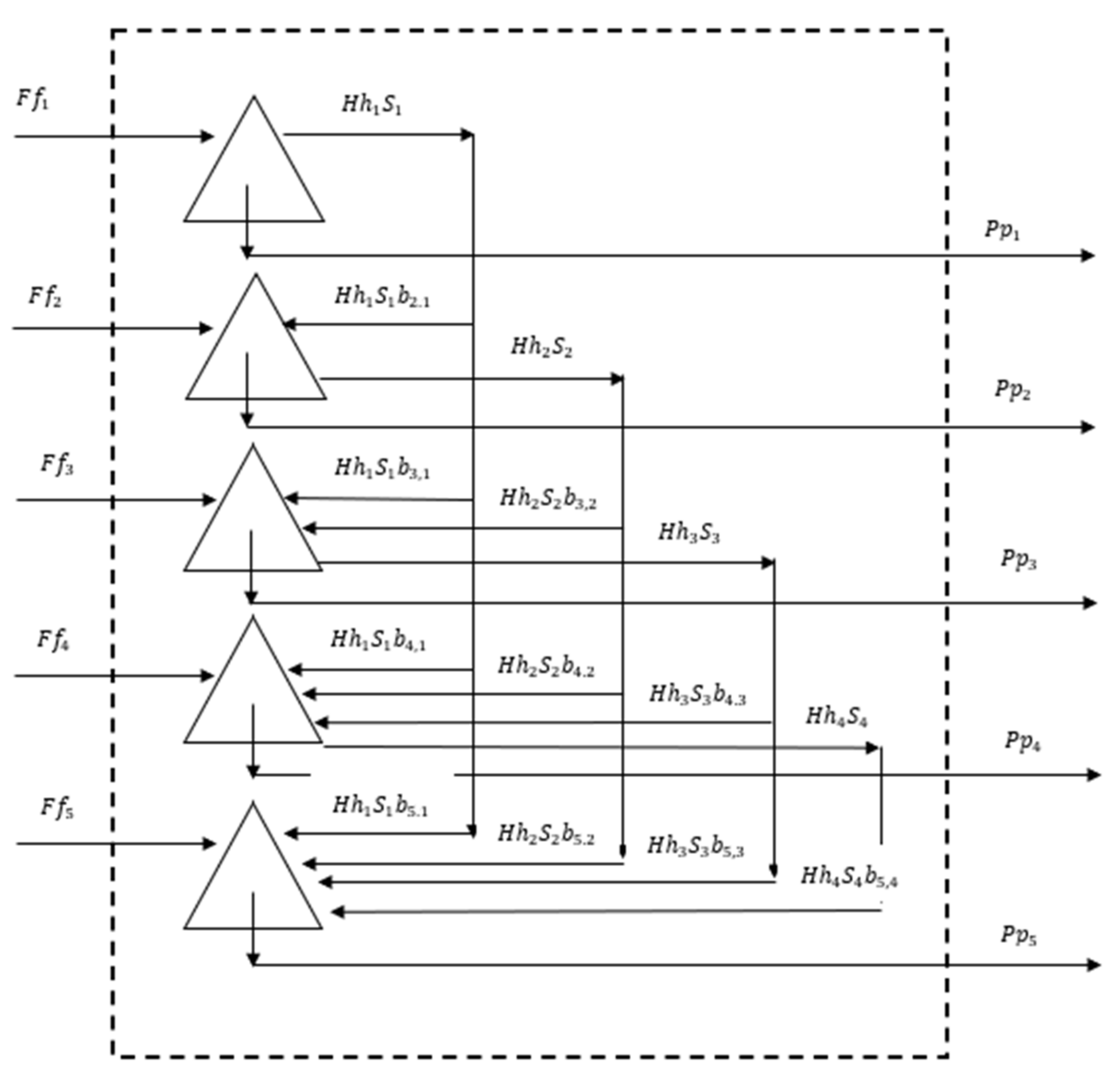
It is important to understand the difference between the classic size-mass balance model and the simple model. The classic size-mass balance model is illustrated in the diagram in Figure 1.

The perfectly mixed mill region represented in Figure 1 is being fed F t/h of coarse particles and producing P t/h of finer particles. Each triangle represents a particle size range in the perfectly mixed region. There is no special location associated with each size range, but, in the diagram, the coarsest particles are represented by the top triangle. The lower the position of the triangle in the sketch, the finer the particle size range it represents.

For the fourth size class, accounting for all particles leaving the size class in the left side of the equation and all particles entering the class in the right side of the equation:

$$H{h}_4{S}_4+P{p}_4=F{f}_4+H{h}_1{S}_1{b}_{4,1}+H{h}_2{S}_2{b}_{4,2}+H{h}_3{S}_3{b}_{4,3}$$

(1)

At steady state, F = P. Furthermore, for a perfectly mixed region, h_i = p_i. Equation (1) can be rewritten as:

$$H{p}_4{S}_4+F{p}_4=F{f}_4+H\left(p_1{S}_1{b}_{4,1}+p_2{S}_2{b}_{4,2}+p_3{S}_3{b}_{4,3}\right)$$

Dividing both sides by F, and rewriting the sum within parenthesis using sigma notation:

$$\frac{H}{F}{p}_4{S}_4+p_4=f_4+\frac{H}{F}{\displaystyle \sum }_{j=1}^{4-1}{p}_j{S}_j{b}_{4,j}$$

The ratio H/F is equal to τ, the average residence time in the perfectly mixed region. Solving for p₄:

$$p_4\left(\tau S_4+1\right)=f_4+\tau {\displaystyle \sum }_{j=1}^{4-1}{p}_j{S}_j{b}_{4,j}$$

$$p_4=\frac{f_4+\tau {{\displaystyle \sum }}_{j=1}^{4-1}{p}_j{S}_j{b}_{4,j}}{\tau S_4+1}$$

It can be readily seen that this expression can be written in a general form for any size class i within the perfectly mixed region:

$$p_i=\frac{f_i+\tau {{\displaystyle \sum }}_{j=1}^{i-1}{p}_j{S}_j{b}_{i,j}}{\tau S_i+1}$$

(2)

Equation (2) represents the population balance model solution for a continuous, perfectly mixed mill region. It is in fact a size-mass balance with all distributions as mass-weighed distributions rather than the number-weighed distributions that are used in formal population balance models. Equation (2) can be solved recursively starting with size i = 1.

The solution in Equation (2) can be easily expanded to a series of perfect mixers in series, with each mixer fed with the product of the previous one.

Classification effects can be incorporated as well, and this is required in overflow ball mills that are operated with relatively lower slurry viscosities, in which case overflow classification becomes important, and in grate discharge mills, such as ball mills, ROM mills and SAG mills.

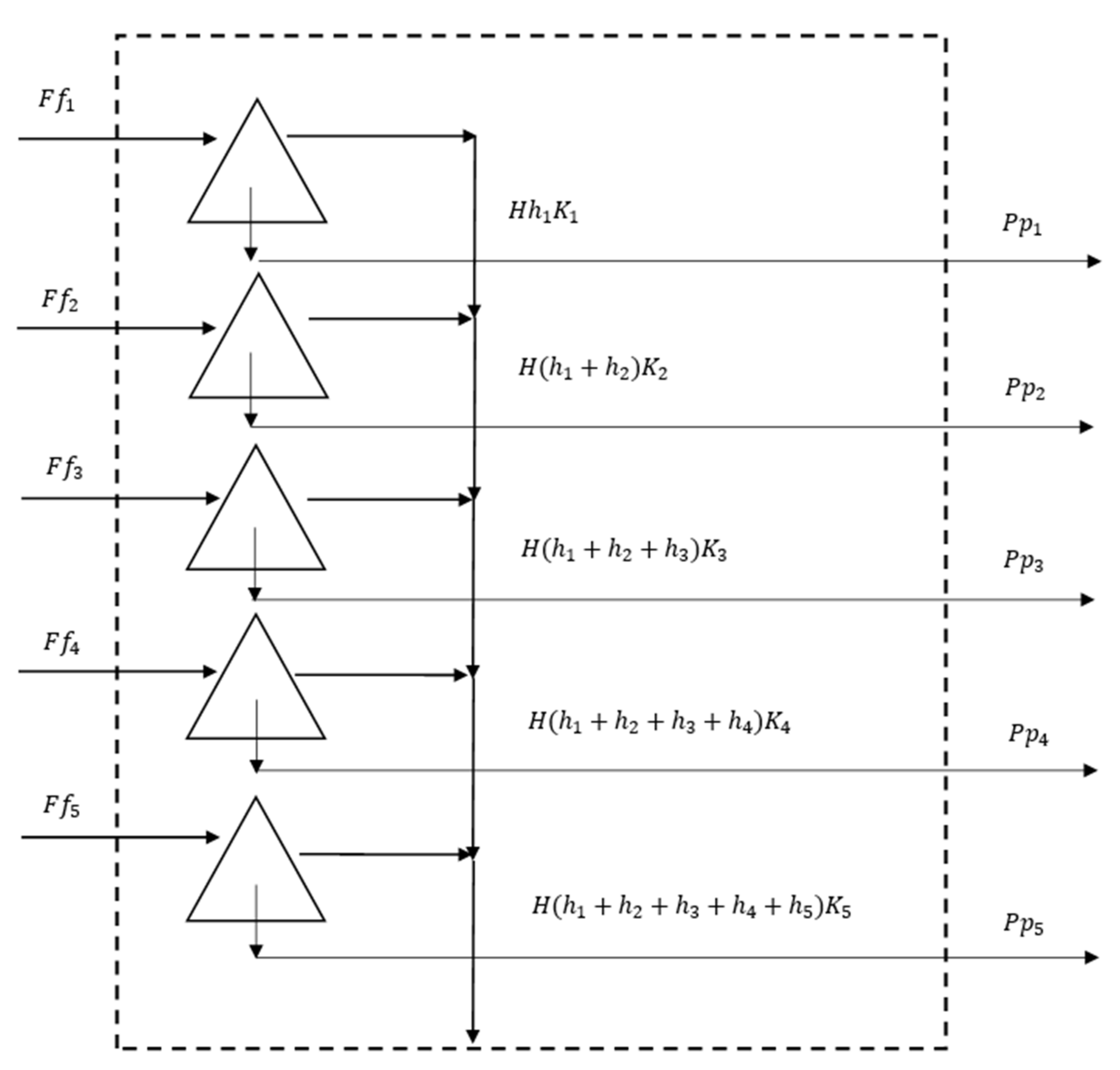
For the simple model it is not necessary (nor desirable) to be concerned with the destinations of all breakage products (the breakage function). All that we are concerned with is the rate of breakage of all particles larger than a given size. A diagram could be envisaged for this model in the same fashion as the diagram for the classic model. This is shown in Figure 2.

For the simple model, the same definitions as in the classic model in Figure 1 are used, except that here the rates of breakage of each size class S_i are replaced by cumulative rates K_i as we are only interested in the rate of production of particles smaller than size i from all particles larger than size i. It is worth pointing out that K₁ = S₁ and K_i ≠ S_i for i > 1.

Similarly, a balance for the fourth size class can be written as:

$$F{f}_4+H\left(h_1+h_2+h_3+h_4\right)K_4=P{p}_4$$

(3)

Again, at steady state, F = P. Furthermore, for a perfectly mixed region, h_i = p_i. Equation (1) can be rewritten as:

$$F{f}_4+H\left(p_1+p_2+p_3+p_4\right)K_4=F{p}_4$$

$$f_4+\frac{H}{F}\left(p_1+p_2+p_3+p_4\right)K_4=p_4$$

Using the definition of the cumulative distribution for the sum within the parenthesis:

$$f_4+\tau \left(1-P_4\right)K_4=p_4$$

(4)

and for any size i, Equation (4) can be generalized to:

$$f_i+\tau \left(1-P_i\right)K_i=p_i$$

(5)

This is the simple model for a perfectly mixed region of a continuous grinding mill, as proposed by Gaudin and Meloy [4]. More recently, the simple model was revisited to make estimates of the charge in a SAG pilot mill [5]. In that work the cumulative rates were assumed to be constant or highly independent of the hold-up size distribution, and this apparently worked well for predicting the charge level under distinct grinding conditions, with power draw as the driving charge level regulator.

2. Test Methods

Although Duffy gives a complete description of the mill and test methods, a summary is given here for convenience. Figure 3 shows a typical illustration of the mill. The vertical drive shaft is fitted with one or two spirals that circulate slurry (water and ore) and media (steel balls) from the bottom of the mill to the top of the spiral, where they overflow and are recirculated to the bottom. A region above the top of the spiral acts as a settling region and finer material leaves the mill overflow as product. When used in the batch mode this overflow is pumped back to the base of the mill without external classification. The test starts by loading a measured amount of slurry with a known solid concentration and particle size distribution into the mill until the mill is filled. The mill is then started, slurry circulates via the overflow return pipe and samples are taken from the recycling output at suitable time periods.

Provided that the volume of the sample taken is small compared to the total volume in the mill, this is exactly like a normal batch test except it is not necessary to stop and empty the mill to take a sample. If the recirculation rate is sufficiently high (see below) then the product sample will be representative of the variation of the size distribution of the mill contents with time. There is little change in hold up or slurry density during the test. The mill size is given as about 1.1 m high and 0.24 m wide, and it was manufactured by the Kubota Tower Mill Corporation.

3. Mill Conditions

The measured conditions in the mill for each of the nine tests are given in

Table 1. Measured mill conditions.

Run No.	Ball Dia. mm	Ball Load kg	Slurry Conc. wt.% Solids	Slurry Weight kg
1	9	110	59	153
2	9	110	47.5	132.5
3	12.7	110	54.8	131
4	12.7	130	52.5	125.5
5	12.7	150	49.4	122
6	12.7	150	54.2	132
7	12.7	150	64.3	134.5
8	12.7	150	57.4	132
9	12.7	150	49	130.5

.

For a mill of this size, it is convenient to work in units of kg and liter, with densities expressed as kg/L (=g/cm³ = specific gravity). Let the ball diameter be d (mm), the load of balls be BL (kg), the slurry (often called pulp) concentration be s (weight % solids or weight fraction of solids) and the charge of slurry (ore and water) be pulp weight (kg). The density of the steel balls is given as 7.9 kg/L and the ore as ρ_ore = 3.82 kg/L.

These values can be expressed as derived values using definitions similar to those used in tumbling ball mills [6]. Let W be the weight of ore in the charge (referred to as the hold up), J be the fraction of the mill volume filled by a bed of balls at rest with a formal porosity of 40% and U be the fraction of this bed porosity that is filled by the ore particles as a bed, also with a formal porosity of 40%. Let the active volume of the mill be defined as V = the combined volume of slurry and balls (liters). Then:

• pulp density = 1/[(s/ρ_ore) + (1 − s)]
• pulp volume = pulp weight/pulp density
• volume of balls = ball load/ball density
• total volume = pulp volume + ball volume
• hold up W = pulp weight × slurry concentration as weight fraction of ore
• J = (ball volume/0.6)/total volume
• U = (W/ore density)/ball volume

The measured values obtained by Duffy produce the data given in

Table 2. Derived mill conditions.

Run No.	Mill Volume (L)	Pulp Density (kg/L)	W (kg)	J (-)	U (-)	T (min)
1	100.4	1.77	90.3	0.24	1.7	N.A
2	100	1.54	62.9	0.24	1.18	0.7
3	91.9	1.68	71.8	0.24	1.35	0.8
4	93.4	1.63	65.9	0.28	1.05	0.7
5	96.7	1.57	60.3	0.33	0.83	0.9
6	98	1.67	71.5	0.33	0.99	1
7	89.4	1.91	86.5	0.33	1.19	N.A
8	94.8	1.74	75.8	0.33	1.04	1.1
9	102.6	1.56	64	0.33	0.88	0.7

.

It can be seen that expressing the mill conditions in a form similar to that used for tumbling ball mills gives values very similar to the conditions used in ball mills to get optimum performance, especially U being close to 1 for most of the runs. The mean active mill volume determined from the amount of slurry and balls necessary to fill the mill to overflow is 96.4 L, which is consistent with the physical dimensions of the mill, and the variation of values from the mean is believed to be consistent with the expected variation in experimental determination of the inputs.

Furthermore, considering the pumped flow rates of overflow back to the mill, each liter of flow contains:

• liters of solids = slurry conc./[slurry conc. + ρ_ore (1 − slurry conc.)]
• kg of solids = liters of solids × ρ_ore

Thus, knowing the volume flow rate of slurry, the weight flow rate of solids can be calculated. The mean residence time of solids in the mill is defined by τ = W/(weight flow rate of solids) and these results are also shown in Table 1 for those tests where flow rates are available in Duffy’s thesis.

The values of the volume flow rate are somewhat variable with the test time, but the estimates of mean residence time show that the solids being ground circulate at least once per minute. Since the first test time is 15 min this seems an adequate justification for a fully mixed mill.

All tests were carried out with the same stirrer speed of 100 rpm.

4. Preliminary Analysis of the Kinetics of Size Reduction

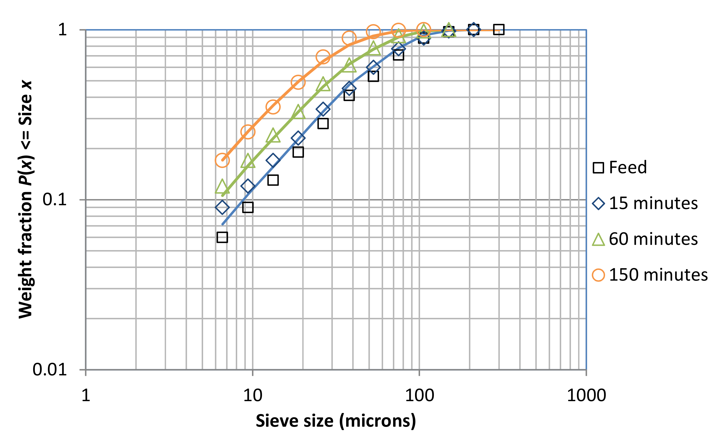
The kinetics of size reduction is determined from the rate at which the particle size distribution of the feed is reduced to smaller particle sizes. The symbolism to describe the size distributions is as follows. Let the particle size distribution of the material (being ground) in the mill at zero grinding time (the feed) be described by the cumulative fraction by weight F_i less than size x_i, where x is a sieve size (or equivalent) in microns and i is an integer indexing a 1/√2 size interval with the upper size of x_i, with i ranging from 1 for the largest size to n, where n is the number of size intervals. Thus, the nth interval is size x_n to 0 (known as the sink interval). Similarly, let the product size distributions P_i,k be defined for a series of grinding times t in minutes indexed by the integer k, starting with 1, i.e., t₁, t₂, …t_k.

Table 3. Particle size distributions of feed and product for Run 1, x in microns, t = 15, 30, 60, 90, 120, 150 min.

xi	Fi	Pi,1	Pi,2	Pi,3	Pi,4	Pi,5	Pi,6
300	1	1	1	1	1	1	1
212	0.998	0.997	0.999	1	1	1	1
150	0.97	0.976	0.991	0.997	0.999	0.999	1
106	0.886	0.889	0.959	0.983	0.994	0.996	0.999
75	0.712	0.769	0.845	0.92	0.963	0.979	0.994
53	0.534	0.6	0.677	0.781	0.873	0.914	0.966
38	0.407	0.448	0.517	0.624	0.749	0.791	0.89
26.5	0.285	0.338	0.378	0.477	0.541	0.593	0.687
18.8	0.189	0.235	0.256	0.33	0.372	0.414	0.488
13.3	0.129	0.17	0.179	0.236	0.265	0.295	0.349
9.4	0.092	0.12	0.128	0.168	0.186	0.21	0.246
6.6	0.063	0.085	0.091	0.116	0.128	0.147	0.168

shows the results for Run 1:

Examination of these data indicated that the results fitted the “simple” model of batch grinding kinetics [4,7]. This model results from a compensation condition where larger particle sizes break more quickly than smaller sizes but the fraction of their breakage products that is smaller than a chosen size x (less than the breaking sizes) is lower, to the extent that the rate of production of material smaller than size x depends on the amount of material larger than size x but NOT on the size distribution of the larger sizes. The normal batch grinding equation then becomes:

rate of increase of mass of particles less than size x_i = sum of all contributions from breakage of larger sizes

that is:

$$\frac{dP\left(x_i,t\right)}{dt}W={\displaystyle \sum }_{j=1}^{i-1}{B}_{i,j}{S}_j{w}_{j}W$$

(6)

where:

w_j is the fraction of the hold up W that has particle sizes in the size interval indexed by j.

B_i,j is the primary cumulative breakage distribution function (i.e., the mass fraction of products broken from the size interval indexed by j that have sizes less than or equal to particle size x_i).

S_j is the specific rate of breakage of particles in the size range of interval j, j < i. Since the compensation condition states that B_i,j S_j is a function of x_i only, B_i,j S_j can be replaced by S(x_i). This now has the meaning of the specific rate of breakage of all sizes larger than x_i.

Since S(x_i) is a constant for a chosen x_i it can be taken out of the summation, while W cancels and the sum of w_j is the fraction of the particle mass that is greater than or equal to size x_i; i.e., 1 − P(x_i,t). Separating and integrating Equation (6) from t = 0 to t = τ with these changes and using the initial condition of 1 − P(x_i,0) = 1 − F(x_i) gives the simple model equation for batch grinding:

$$\begin{array}{cc}P\left(x_i,\tau \right)=1-\left[1-F\left(x_i\right)\right]\exp \left(-S_{i-1}\tau \right)\hfill & i>1\\ \hspace{1em}\hspace{1em}\hspace{1em}\hspace{0.17em}=1\hfill & i=1\end{array}$$

(7)

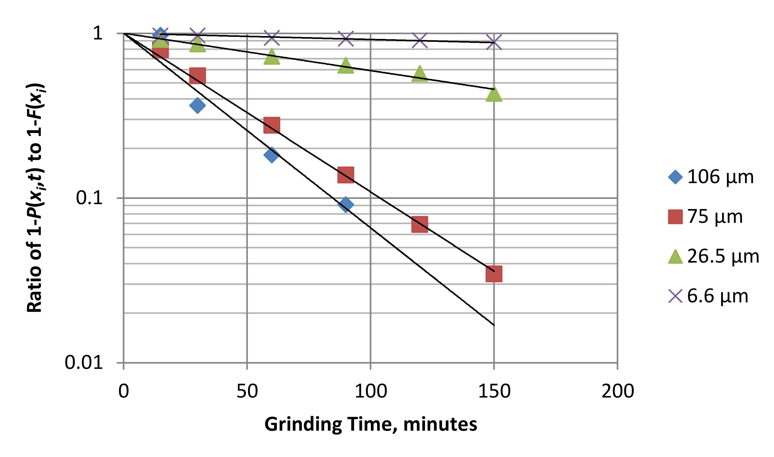
The applicability of this equation to the data can be tested by plotting (1 − P)/(1 − F) for chosen particle sizes, on a log scale, versus τ on a linear scale, as shown in Figure 4. There is scatter in some of the results, but the general pattern is that the model describes the data with reasonable precision. Note that P_i depends on S_i−1 not S_i, as P₂ clearly depends on S₁. Furthermore, Equation (7) is continuous in grinding time t but discrete in size x.

The simple solution for batch grinding for time t is:

$$\begin{array}{cc}1-P\left(x_i,t\right)=(1-F_i)\exp \left(-S_{i}t\right)\hfill & i>1\\ \hspace{1em}\hspace{1em}\hspace{1em}\hspace{1em} =0\hfill & i=0\end{array}$$

(8)

This can be plotted as the fraction 1 − P(x_i,t)/(1 − F_i) versus grinding time t. It is algebraically convenient to denote the ratio 1 − P(x_i,t)/(1 − F_i) as Y(i,t):

$$Y\left(i,t\right)=\exp \left(-S_{i}t\right)$$

(9)

where t is a suitable range of time values. Therefore, a plot of Y(i,t) versus t on a log-linear scale will give a straight line. Similarly, X_i,k is defined as the matrix of experimental values of (1 − P_i,k)/(1 − F_i), with k indexing the (discontinuous) values of experimental grinding times. S_i is adjusted to match the experimental values for a chosen i (i.e., a chosen x_i). This is repeated for different sizes. A good fit to the experimental values of X_i,k will show if the simple model applies and the vector of S_i values can be obtained.

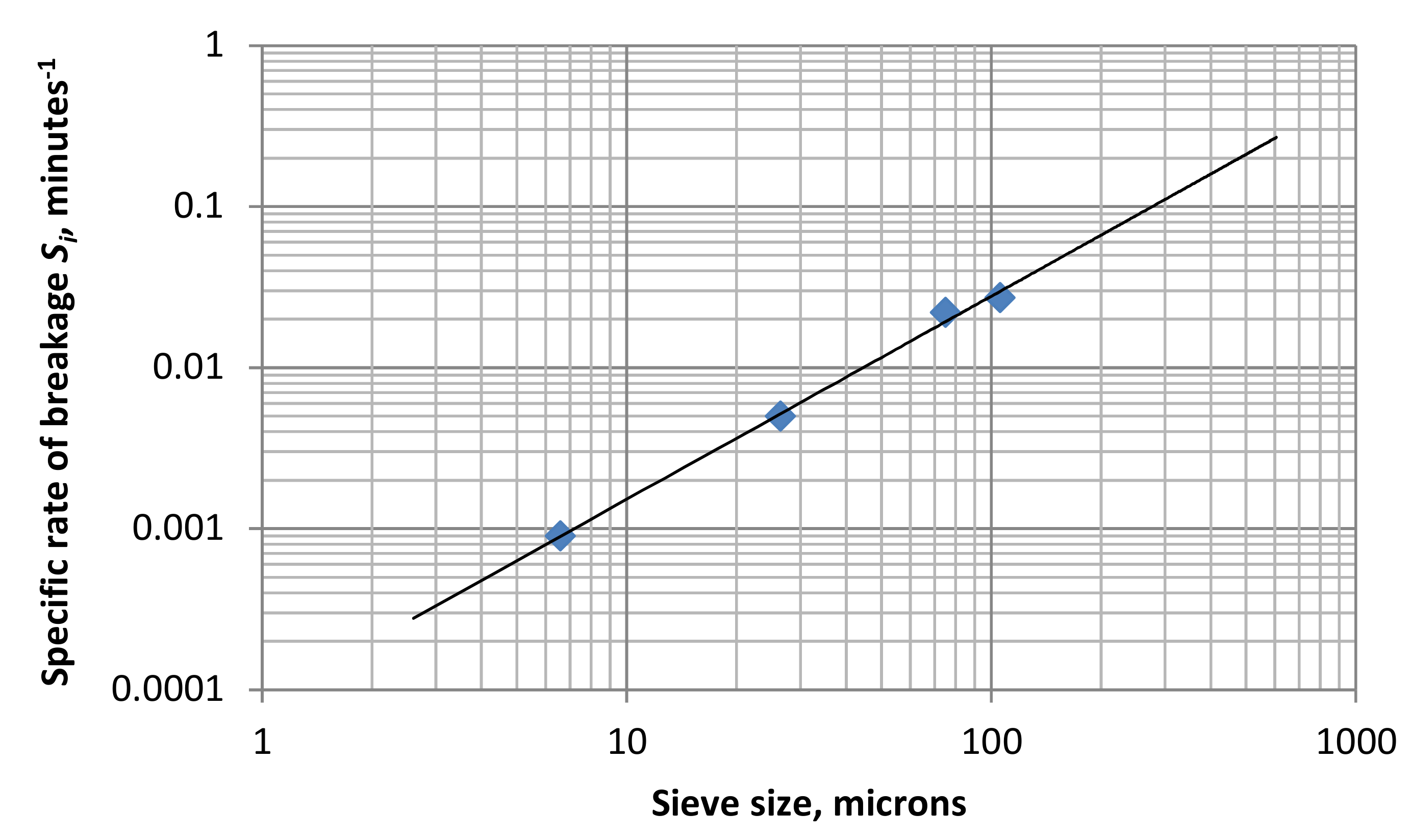
Figure 5 shows that the relation can be expressed as:

$$S\left(x\right)=a{\left(\frac{x}{x_s}\right)}^{\alpha }, a=7.5 \times {10}^{-5}, \alpha =1.27, x_s=1$$

(10)

It should be understood that x_s is a standard size, 1 micron in this case, so x/x_s is dimensionless and a has units of fraction per minute; i.e., min⁻¹. It is common to leave out x_s as its value is one, but its inherent presence must be remembered to avoid confusion with units.

In the simple model of grinding kinetics, S(x) has the meaning of the specific rate of breakage (fraction per unit time) of all particles greater than size x to sizes less than or equal to size x. Thus, a and α are characteristic parameters that vary with mill conditions and the material being ground. The cumulative primary breakage distribution B is dimensionally normalized and is:

$$B\left(x,y\right)={\left(\frac{x}{y}\right)}^{\alpha } y\ge x$$

(11)

Then, as:

$$\begin{gathered} S\left(y\right)=a{y}^{\alpha } \\ B\left(x,y\right)S\left(y\right)=a{x}^{\alpha } \end{gathered}$$

(12)

Equation (12) is the compensation condition that is necessary for the simple model to be valid [7]; i.e., SB is a function of x but not of larger size y. Equation (10) can be expressed as:

$$S_i=a{\left(x_i\right)}^{\alpha }$$

(13)

Equation (7) gives:

$$P{C}_{i,k}=1-\left(1-F_i\right)exp\left(-S_i{t}_k\right)$$

(14)

where PC is the computed model value.

In addition to the methods of determining a and α given above, the values can be found by assuming the model to apply (as indicated here) and choosing values for a and α that give the best fit between the computed and experimental values of the product size distributions, as is shown in Figure 6. The criterion chosen here is unweighted least squares of error (as described in the Statistical Analysis in Section 6):

difP_i,k = P_i,k − PC_i,k

(15)

$$W{S}_{i,k}=\overrightarrow{{\left(\mathrm{dif}{P}_{i,k}\right)}^2}$$

(16)

$$SSQ={\displaystyle \sum }_k{\displaystyle \sum }_{i}W{S}_{i,k}$$

(17)

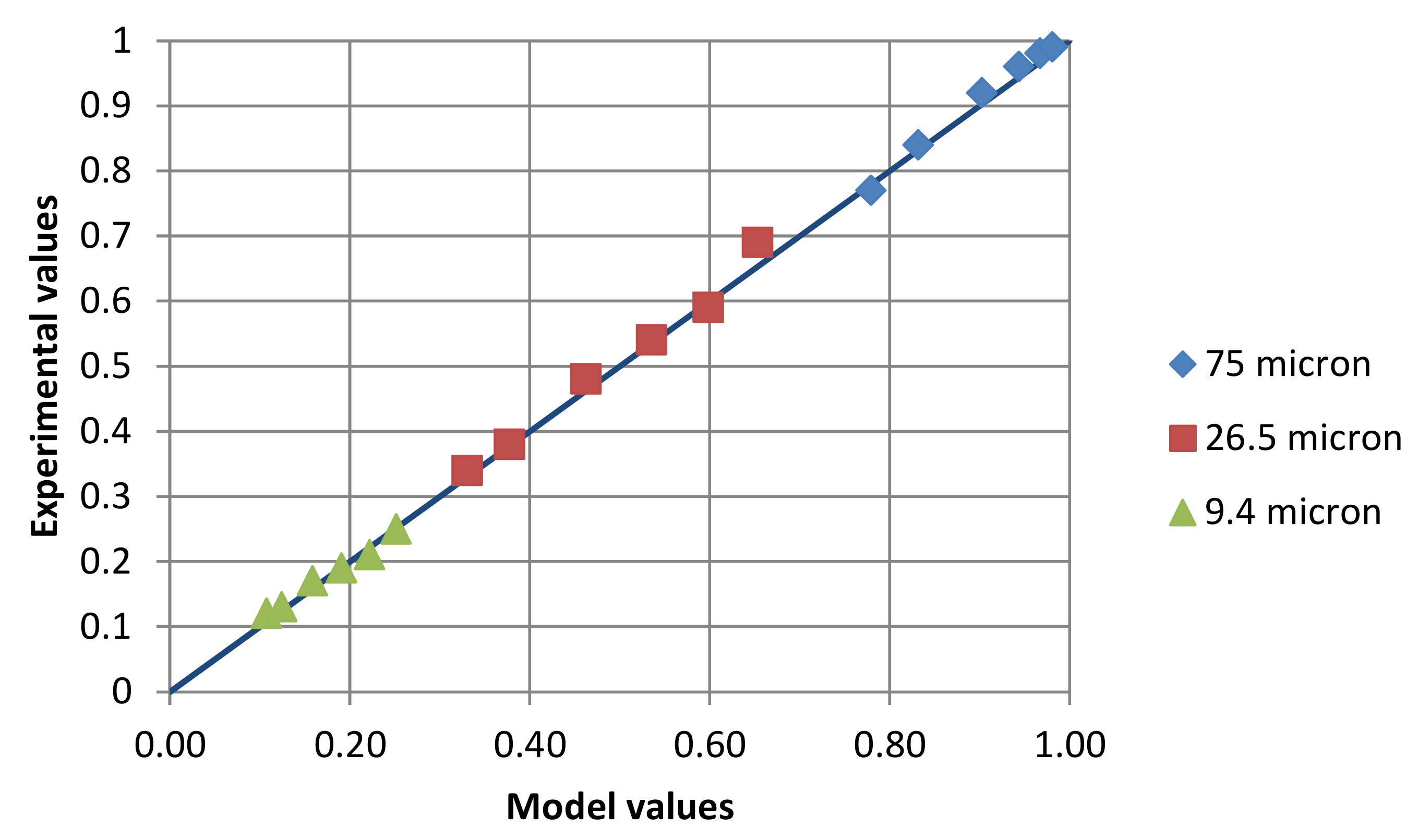
The adequacy of the fit with the simple model can also be demonstrated by comparing measured and calculated % < size for selected sizes for all grinding times. This is shown in Figure 7. The slope of the straight line in this figure is 1, passing through 0, and there is very little scatter for the selected particle sieve sizes.

5. Results for All Runs

Table 4. Estimates of the simple model parameters.

Run No.	a (min−1)	α	SSQ	Slurry Conc. (wt. % Ore)
1	7.6 × 10−5	1.27	0.021	59
2	2.6 × 10−5	1.7	0.019	47.5
3	2.7 × 10−5	1.5	0.039	54.8
4	3.0 × 10−5	1.5	0.028	52.5
5	2.0 × 10−5	1.7	0.025	49.4
6	1.3 × 10−5	1.8	0.014	54.2
7	3.0 × 10−5	1.5	0.218	64.3
8	4.0 × 10−5	1.5	0.059	57.4
9	2.0 × 10−5	1.8	0.022	49.0

gives the results for a and α plus the SSQ criterion value for each run.

It can be seen that Run 7 has an SSQ several times higher than the other values. There was nothing unusual about the test conditions, but Duffy reported that the mill appeared to be blocking during this run. Consequently, Run 7 was ignored in further analysis of the results. It can be observed that the values of α are 1.5 plus or minus about 0.3. It is expected that the a values should vary with slurry density (see below) but there is no physical reason why changes in slurry density would make smaller particles break slower or faster with respect to larger particles, so the value of α should be constant. In addition, it has been shown [8] that determination of parameters in the presence of variability in the data can give ranges of the parameter values that are equally valid. A discussion in detail of the application of statistics to the determination of kinetic breakage parameters is given in Austin, Klimpel and Luckie, [9].

Consequently, the data for Run 1 were re-examined to see if the use of α = 1.5 would give a statistically significant worse result than α = 1.27. For any value of α the value of a that gives the minimum SSQ is found by a search, and α is also searched to get the optimum minimum.

Trial values of a and α for Run 1 are:

• SSQ = 0.019 for α = 1.27, a = 7.9 × 10⁻⁵;
• SSQ = 0.014(5) for α = 1.4, a = 5.2 × 10⁻⁵;
• SSQ = 0.016 for α = 1.5, a = 3.7 × 10⁻⁵;
• SSQ = 0.027 for α = 1.6, a = 2.5 × 10⁻⁵.

It can be seen that there is a range of a, α pairs that give little change in SSQ values. The optimum minimum was for α = 1.45, a = 4.4 × 10⁻⁵, giving SSQ = 0.014(5).

6. Statistical Analysis

In order to see if the value of α = 1.5 was valid, a statistical analysis [9] was adapted to apply to the simple model. Since this model considers a kinetic mass-time balance for breakage of material greater than sieve size x to product less than size x, the correct definition of error is P_i − PC_i. In this model there are only two parameters, a and α. An investigation was made of weighting factors as follows.

Values of error could have had a bias of becoming larger error values at higher 1 − PC values. However, the error values were so variable that it was not possible to decide on the weighting relation with a graphical examination, so a least squares search was undertaken. The objective was to minimize the sum of squares of error taken over all the data points with a suitable weighting factor.

$$SSQW={\displaystyle \sum }_k{\displaystyle \sum }_i\left[\frac{{\left(\mathrm{dif}{P}_{i,k}\right)}^2}{\left[{\left(1-P{C}_{i,k}\right)}^{\gamma }\right]}\right]$$

(18)

The value of γ was varied from 0 to 2, giving: γ = 0, SSQW = 0.014; γ = 1/2, SSQW = 0.032; γ = 1, SSQW = 0.097; γ = 1.5, SSQW = 0.56; and γ = 2, SSQW = 9.9. The results suggest that there is no weighting factor; that is, γ = 0 and the sum of squares is of “absolute error squared”; γ = 2 would give “relative error squared”.

The values of a and α that give the minimum SSQ are called “optimal” and the corresponding SSQ is the optimal value. Then, the F factor is defined as

$$F=\frac{\left(\frac{SSQ}{n-N+1}\right)}{\left(\frac{SSQopt}{n-N}\right)}$$

(19)

In this equation, n is the number of data points and N is the number of parameters being searched. Each test had 12 data points and 6 times, so n = 72. N is 2 for a and α, but when α is set (at 1.5 in this case) then SSQ has N replaced by N − 1. Examination of a table of F values [10] as a function of Q(F|ν1,ν2) where ν1 = n − N, ν2 = n − N + 1 and Q is the probability that SSQ > SSQopt, will show if the SSQ error from forcing alpha to be 1.5 is significantly greater than SSQopt, according to where F is placed in the table.

For the case considered here, the value of F < 1.5 (95% confidence level) implies that SSQ is not significantly greater than SSQopt.

Table 5. The “F-Test” results for Runs 1 to 9.

Run	α	a	SSQopt	α	a	SSQ	F
1	1.45	4.4 × 10−5	0.014	1.5	3.7 × 10−5	0.016	1.12
2	1.7	2.6 × 10−5	0.019	1.5	4.8 × 10−5	0.028	1.45
3	1.4	3.7 × 10−5	0.012	1.5	3.7 × 10−5	0.013	1.07
4	1.65	1.7 × 10−5	0.024	1.5	3.0 × 10−5	0.028	1.15
5	1.7	2.0 × 10−5	0.025	1.5	3.85 × 10−5	0.037	1.46
6	1.8	1.3 × 10−5	0.014	1.5	3.5 × 10−5	0.018	1.28
7	Excluded
8	1.6	2.8 × 10−5	0.028	1.5	3.95 × 10−5	0.029	1.03
9	1.8	2.0 × 10−5	0.009	1.5	4.85 × 10−5	0.021	2.30

gives the results of applying Equation (19) to all tests (except Run 7).

It is seen that the F value is less than 1.5, a requisite to conclude that there is no significant error introduced by using α as 1.5 with the corresponding a values, except in Run 9. Thus, it was decided to choose α as 1.5 for all runs and therefore to use only the values of a to correlate the effects of test conditions on specific rates of breakage.

7. Summary and Conclusions

(1)

The data give strong evidence that the kinetics of size reduction in this batch grinding system can be fitted with the simple model of first-order breakage. It must be emphasized that this very special form of the general equations for the kinetics of grinding has not been found to apply to other mills, such as tumbling ball mills, rod mills, etc., either in our own experience or in that of others (to the best of our knowledge). In fact, it has generally been used only to illustrate the concepts involved. It is possible that the condition in Equation (12) holds reasonably well for the range of sizes covered by Duffy’s tests. Figure 6 shows a slight degree of deviation from the measured size distributions that may be due to model deficiency, but it is also possible that this is just the result of the highly restricted number of parameters (only one) that were allowed to vary. Further work is required to verify if the simple model can be applied to other grinding systems (with different mill types, grinding conditions and ores).

(2)

The model requires only the determination of two parameters, a and α, to calculate the specific rates of breakage for any set of mill conditions. This makes it possible to determine the parameters with simple search methods, using only the feed and product size distributions.

(3)

Statistical analysis of the data from nine test runs, with the variables ball load, ball diameter and slurry density, showed that a value of α = 1.5 could be used for seven of the nine runs.

(4)

There seems to be no reason to doubt that the model can be extended to steady state continuous operation of the mill, as is done by extending the batch grinding kinetics of a laboratory or pilot-scale ball mill to the operation of a full-scale [11].

(5)

It is necessary in progressing from batch testing to continuous operation to allow for exit classification due to sedimentation in the upper part of the continuous mill. The data were not sufficient to make any estimates of exit classification because no samples were taken from the sedimentation zone, only from the overflow.

(6)

In addition, it will be necessary to determine a residence time distribution for this type of mill, as well as methods for scale-up to full-scale mills, probably via net mill power. These factors will be considered in future parts of our work.

(7)

As in tumbling ball mills, the positive value of α shows that larger particle sizes are broken more rapidly than small particles.