Article

Development and Description of a Composite Hydrogeologic Framework for Inclusion in a Geoenvironmental Assessment of Undiscovered Uranium Resources in Pliocene- to Pleistocene-Age Geologic Units of the Texas Coastal Plain

by
Andrew P. Teeple
1,*,
Kent D. Becher
2,†,
Katherine Walton-Day
3,
Delbert G. Humberson
4 and
Tanya J. Gallegos
5
1
Oklahoma-Texas Water Science Center, U.S. Geological Survey, 1505 Ferguson Lane, Austin, TX 78754, USA
2
Oklahoma-Texas Water Science Center, U.S. Geological Survey, 501 W. Felix St. Building 24, Fort Worth, TX 76115, USA
3
Colorado Water Science Center, U.S. Geological Survey, P.O. Box 25046, MS 415, Lakewood, CO 80225, USA
4
International Boundary and Water Commission–United States Section, 4191 North Mesa St., El Paso, TX 79902, USA
5
Energy and Minerals Science Center, U.S. Geological Survey Geology, 12201 Sunrise Valley Drive, Reston, VA 20192, USA
*
Author to whom correspondence should be addressed.
Kent D. Becher is now retired.
Minerals 2022, 12(4), 420; https://doi.org/10.3390/min12040420
Submission received: 12 February 2022 / Revised: 23 March 2022 / Accepted: 24 March 2022 / Published: 29 March 2022
(This article belongs to the Special Issue Environmentally Sound In-Situ Recovery Mining of Uranium)

Abstract

:
A previously completed mineral resources assessment of the Texas Coastal Plain indicated the potential for the future discovery of uranium resources. Geoenvironmental assessments that include the hydrogeologic framework can be used as a tool to understand the potential effects of mining operations. The hydrogeologic framework for this study focused on the composite hydrogeologic unit of the tract permissive for the occurrence of uranium consisting of the upper part of the Miocene-age Fleming Formation/Lagarto Clay, Pliocene-age Goliad and Pleistocene-age Willis Sands, Pleistocene-age Lissie and Beaumont Formations, and Holocene-age alluvial sediments (fluvial alluvium and eolian sand deposits). This composite hydrogeologic unit, which contains the Chicot and Evangeline aquifers of the Gulf Coast aquifer system, is intended for inclusion in a regional-scale geoenvironmental assessment of as yet undiscovered uranium resources. This article provides (1) a brief literature review describing the geologic and hydrogeologic settings, (2) the methodology used to develop a composite hydrogeologic framework, and (3) descriptions and maps of the land-surface altitude, composite hydrogeologic unit base and midpoint depth, water-level altitude, depth of water, unsaturated and saturated zone thickness, and transmissivity and hydraulic conductivity. A composite hydrogeologic unit, created by combining geologic and hydrogeologic data and maps for individual geologic and hydrogeologic units, is intended for use as a tool in a geoenvironmental assessment to evaluate potential contaminant migration through various avenues. Potential applications include using the hydrogeologic framework as an input into a geoenvironmental assessment to help estimate the potential for (1) runoff of contaminants into surface water, (2) infiltration of contaminants into the groundwater (aquifers), or (3) movement of contaminants from the mining area through wind, groundwater-flow, or streamflow in a given permissive tract. The procedures outlined in this paper also provide a method for developing hydrogeologic frameworks that can be applied in other areas where mining may occur.

1. Introduction

In 2015, the U.S. Geological Survey (USGS) completed a mineral resources assessment of the Texas Coastal Plain [1]. Results from this assessment indicated there is an estimated 100 million kilograms of recoverable uranium oxide remaining within geologic regions, or tracts, that are referred to as “permissive” because of their perceived favorable characteristics for the occurrence of undiscovered uranium (U) resources (Figure 1). Three permissive tracts were identified based on the extents of the selected geologic units in the Texas Coastal Plain: (1) the Eocene-age Claiborne and Jackson Groups, (2) the Oligocene-age Catahoula Formation and Miocene-age Oakville Sandstone, and (3) the Pliocene-age Goliad Sand and Pleistocene-age Willis Sand and Lissie Formation (Figure 2).
A geoenvironmental assessment may serve as a preliminary tool to predict the potential environmental effects of future mining sites. Historically, uranium deposits in the Texas Coastal Plain were mined in shallow open pits beginning in 1960 [2]. Since 1975, there has been a transition from open-pit mining to in situ recovery (ISR) where uranium is extracted from deeper sandstone-hosted uranium deposits, and currently (2022), all uranium in Texas is produced using ISR [2,3]. ISR is a form of solution mining which uses a chemical solution (lixiviant) to dissolve the uranium orebody in the subsurface (in situ) within a permeable, saturated aquifer, and then the dissolved mixture (pregnant or loaded solution) is pumped to the surface where the uranium can be recovered through further processing [4]. Assuming that future uranium mining reflects the current extensive use of ISR, the following contaminant pathways are prioritized within a given permissive tract for ISR uranium extraction operations: (1) accumulation of radon in air, (2) runoff of contaminants into surface water, (3) infiltration of contaminants into the groundwater (aquifers), and (4) movement of contaminants from the mining area through groundwater-flow or streamflow.
Figure 2. Geologic and hydrogeologic units of the Texas Coastal Plain and the three geologic regions, or tracts, that have favorable characteristics for the occurrence of undiscovered uranium resources, or permissive tracts, as delineated by [1]. Geologic units are modified from [5,6,7,8,9]. Hydrogeologic units are modified from [5,6,10,11]. Permissive tracts are modified from [1]. The Fleming Formation and Lagarto Clay are considered equivalent throughout the study area [9]. The Bigford Formation, El Pico Clay, and Laredo Formation are geologic units of the Rio Grande embayment.
Minerals 12 00420 g002
An understanding of the hydrogeology is needed to better understand the potential for effects of mining on water resources. A hydrogeological framework can be used as input into a geoenvironmental assessment to help estimate the potential for (1) runoff of contaminants into surface water, (2) infiltration of contaminants into the groundwater (aquifers), or (3) movement of contaminants from the mining area through groundwater-flow or streamflow in a given permissive tract. The hydrogeologic framework consists of the lithology, hydrostratigraphy, structural features, and hydraulic properties of one or multiple hydrogeologic units. Because a given permissive tract may consist of multiple geologic and hydrogeologic units, it is useful to build a “composite hydrogeologic unit” that encompasses all hydrogeologic units in a given permissive tract.

1.1. Purpose and Scope

The hydrogeologic framework contains spatial data in the form of maps of land-surface altitudes, thicknesses of geologic units, depths of the hydrogeologic units, water-level altitudes, unsaturated and saturated zone thicknesses of hydrogeologic units, and hydraulic properties (transmissivity and hydraulic conductivity). The purpose of this study was to develop a composite hydrogeologic framework that can be incorporated into a geoenvironmental assessment of the permissive tract consisting of the Pliocene-age Goliad Sand, Pleistocene-age Willis Sand, and Pleistocene-age Lissie Formation that contain the Chicot and Evangeline aquifers of the Gulf Coast aquifer system (Figure 2) [1]. The upper part of the Miocene-age Fleming Formation/Lagarto Clay is included in the composite hydrogeologic unit because this geologic unit has a relatively large sand content and is included as a hydrogeologic unit that contains part of the Evangeline aquifer according to Young et al. [5,6,12]. The Pleistocene-age Beaumont Formation and Holocene-age alluvial sediments (fluvial (water transported) alluvium and eolian (wind-blown) sand deposits) are included in the composite hydrogeologic unit for the permissive tract because of the similarity of their permeabilities to the other units that contain the Chicot aquifer [7]. The collective geologic units of the upper part of the Fleming Formation/Lagarto Clay, Goliad and Willis Sands, the Lissie and Beaumont Formations, and the alluvial sediments that contain the Chicot and Evangeline aquifers, are hereinafter referred to as “permissive tract 3” (Figure 2). The specific objectives of this paper are to provide the following for permissive tract 3: (1) a brief literature review describing the geologic and hydrogeologic settings, (2) the methodology used to develop a composite hydrogeologic framework, and (3) descriptions and maps of the land-surface altitude, composite hydrogeologic unit base and midpoint depth, water-level altitude, depth of water, unsaturated and saturated zone thickness, and transmissivity and hydraulic conductivity.

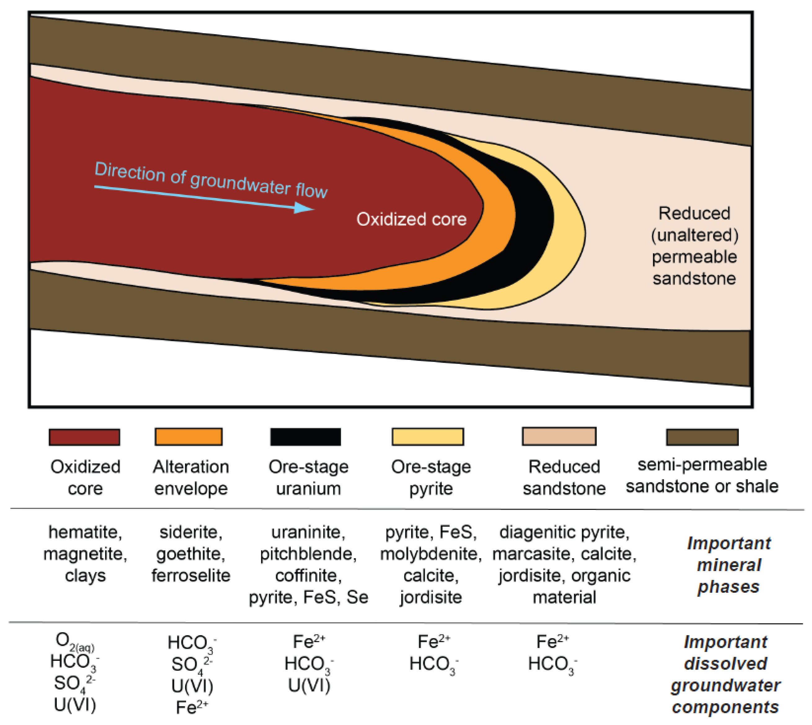
1.2. Geologic and Hydrogeologic Setting

The Texas Coastal Plain is in a broad, flat region of southeastern Texas bordering the Gulf of Mexico (Figure 3). Geologic and climatic factors combine in this region to create conditions favorable for the occurrence of mineable quantities of U hosted by Eocene through Pliocene sandstones [2]. The Texas Coastal Plain features two embayments (Houston and Rio Grande embayments) separated by the San Marcos arch, a subsurface geologic high (Figure 3). The Houston embayment is a subsidence trough centered in southeast Texas, whereas the Rio Grande embayment is a subsidence trough centered on the modern Rio Grande in south Texas. Of the two embayments, the sediments that compose the Rio Grande embayment are thickest. [5,6]. U mineralization in the Texas Coastal Plain occurs in Tertiary-age sandstones that form a curvilinear belt about 600 km (km) long and as much as about 170 km wide (Figure 3). The Texas Coastal Plain includes 254 identified probable U occurrences, including 169 deposits, 79 prospects/showings (73 and 6, respectively), and 4 anomalies [2]. Deposits in the Texas Coastal Plain are generally roll-front deposits hosted in late Eocene to early Pliocene sandstones and are located mostly southwest of the San Marcos arch, in the Rio Grande embayment (Figure 3) [2]. U ore bodies in the Texas Coastal Plain are described as deposited in C-shaped (Figure 4) roll fronts when viewed in cross-section, although individual ore zones have a complex geometry controlled by sand facies variations and background geochemistry [2].
Stratigraphic units in the Texas Coastal Plain form a monocline dipping gently toward the Gulf of Mexico (Figure 4). Tertiary-age sandstones in the Texas Coastal Plain that host U occurrences were deposited either in fluvial-deltaic environments or in marginal marine areas that are collectively part of a more than 14 km thick Tertiary-age wedge of sand, silt, and clay sediments derived from episodic continental scale mountain building and erosion over geologic time [15]. Rapid, massive sediment loading triggered the development of syndepositional growth faults which are associated with both structurally controlled hydrocarbon accumulations and U mineralization [16]. U deposits in the Texas Coastal Plain also are often related to unconformities because they commonly occur within the lower portions of generally porous, regressive units and above impermeable transgressive units that serve as confining units [16].
Permissive tract 3 includes Tertiary to Quaternary-age deposits ranging from the Miocene to the Holocene (Figure 2). Historically, delineation of the geologic units within this age range is difficult because of the lithologic similarity of the sediments and the lack of paleontological control [7]. More recent interpretations have delineated the geologic units with greater confidence using chronostratigraphic correlation [5,6,12,17]. These geologic units include the following formations, from oldest to youngest (Figure 2): the upper part of the Fleming Formation/Lagarto Clay, Goliad Sand, Willis Sand, Lissie Formation (Bentley and Montgomery Formations), Beaumont Formation, and alluvial sediments (fluvial alluvium and eolian sand deposits) (Figure 2). Although the percentage of sand is relatively large in each of these units and no unit definitively functions as a confining unit (the Beaumont Formation might be an exception), there are extensive clay lenses in each unit that may act as confining units at local scales.
Figure 4. Simplified cross section of a uranium roll front showing the upgradient oxidized and downgradient reduced zones (modified from [18]).
Minerals 12 00420 g004

1.2.1. Fleming Formation/Lagarto Clay

The middle to late Miocene-age Fleming Formation/Lagarto Clay contains thick sandstone in the south and northeast and in the near offshore area with relatively less sandstone in the broad middle coast (Figure 2) [5,6]. The Fleming Formation and the Lagarto Clay are equivalent naming designations for the same geologic unit [9]; the Fleming Formation is the more widely used designation, but this paper includes the Lagarto Clay because of the historical use of “Lagarto Clay” in the region, more specifically by Young et al. [5,6,12]. The Fleming Formation/Lagarto Clay is hereinafter referred to as the “Lagarto Clay.” The Lagarto Clay forms a relatively thick low-sand interval in most of the outcrop and near outcrop areas. In the onshore area, the Lagarto Clay is relatively more mud-rich. The Lagarto Clay is part of a major fluvial-deltaic depositional episode where the Lagarto Clay overlies the lower progradational part and forms the upper retrogradational part [5,6]. The Lagarto Clay ranges from about 210 to 430 m thick at outcrop to about 610 to 910 m thick near the coast [5,6]. The Lagarto Clay dips towards the coast at about 10 to 11 m per kilometer (m/km) [5,6]. The Lagarto Clay contains several large fluvial systems ranging from bed-load channel filled sandstones to finer-grained mixed load channel-fill sandstones with varying percentages of sand content of as much as 80 percent in some areas [5,6]. The Lagarto Clay is split into three parts: upper, middle, and lower. The upper part of the Lagarto Clay is of interest because it has more sandstone than the middle part of the Lagarto Clay and has been included as one of the units that contains the Evangeline aquifer [5,6].

1.2.2. Goliad Sand

The Pliocene-age Goliad Sand consists of clay, sandstone, marl, caliche, limestone, and conglomerate [19]. Fluvial deposits within the Goliad Sand consist of very fine to medium sand, gravelly coarse sand, sandy gravel, and pebble-to-cobble-sized gravel depending on location within the fluvial interfingering sequences or facies (Figure 2) [5,6,20]. The Goliad Sand is bound by regional unconformities at the base of massive fluvial sandstones at outcrop and in the shallow subsurface [5,6]. Downdip, the Goliad Sand is bounded by marine transgressive shales [5,6]. The Goliad Sand ranges in thickness from 60 m (m) at outcrop to about 730 m near the modern coastline [5,6]. The Goliad Sand strata dip coastward about 2 to 4 m/km [5,6]. Channel-fill facies are typically composed of 40 to 60 percent sand, whereas interchannel facies are typically composed of less than 20 percent sand, except in the Houston embayment where interchannel facies are often composed of more than 25 percent sand [5,6]. The Goliad Sand is one of the geologic units that contains the Evangeline aquifer (Figure 2).

1.2.3. Willis Sand

At outcrop, the underlying Goliad Sand is erosionally downcut and locally truncated by the Pleistocene-age Willis Sand, and the Willis Sand is in turn eroded and locally onlapped by the overlying Lissie Formation (Figure 2) [5,6,21,22]. At outcrop, in the Houston embayment and along the San Marcos arch, the Willis Sand consists of cuesta-forming erosional remnants, whereas the unit does not crop out into the Rio Grande embayment, although Pleistocene-age deposits are present in the subsurface [5,6]. The sediments of the Willis Sand are described as reddish, coarse, and gravelly sands with subordinate clays that grade into the Goliad Sand in the southwest Gulf Coast of Texas [22,23,24]. The Willis Sand ranges in thickness from about 30 m at outcrop to 150 m near the coast and thickens to the northeast [5,6,25]. The Willis Sand strata dip coastward about 3 to 4 m/km [5,6]. The sand content in the Willis Sand of the central coast of the study area decreases downdip from 70 to 90 percent in the fluvial system to 30 to 70 percent in the deltaic and shore-zone systems [5,9]. The Willis Sand is one of the geologic units that contains the Chicot aquifer (Figure 2).

1.2.4. Lissie Formation (Montgomery and Bentley Formations)

The middle Pleistocene-age Lissie Formation is unconformably contained between the underlying Willis Sand and overlying Beaumont Formation (Figure 2) [5,6,24,26]. North of the Brazos River (Figure 3), the Lissie Formation has been mapped as distinct subunits (the Montgomery and Bentley Formations) (Figure 2) [5,6,27]. In southeast Texas, the Montgomery and Bentley Formations are approximately equivalent to the Lissie Formation, and therefore, the extents of the Montgomery and Bentley Formations are expressed as the extents of the Lissie Formation [7,28]. The Lissie Formation sediments consist of red, orange, and gray fine- to coarse-grained, cross-bedded sands [24], and the formation contains relatively less conglomerate compared to the underlying Goliad Sand [24]. The Lissie Formation ranges in thickness from about 30 m at outcrop to greater than 210 m at the coast [5,6,25]. The Lissie Formation dips coastward about 1 to 4 m/km and is 150 to 300 m deep at the modern coastline [5,6,21,25]. In the central coast of the study area, the sand content in the Lissie Formation is about 50 to 70 percent in the updip fluvial system and about 30 to 70 percent in the downdip shore-zone systems [5,9]. The Lissie Formation is one of the geologic units that contains the Chicot aquifer (Figure 2).

1.2.5. Beaumont Formation

The late Pleistocene-age Beaumont Formation is composed of clay-rich sediments transected by sandy fluvial and deltaic-distribution channels and includes isolated segments of sandy beach ridges parallel to the coast known as the Ingleside barrier/strandplain system (Figure 2) [5,6,26,29]. Although interbedded muddy/shale intervals are generally of similar thickness to the sands, the thickness of individual sands increases updip, whereas the thickness of individual shales increases downdip [5,6]. The Beaumont Formation is contained between the underlying Lissie Formation and overlying Holocene-age alluvial sediments (fluvial alluvium and eolian sand deposits) north of the Brazos River. The Beaumont Formation ranges in thickness from a thin veneer in updip areas to about 150 m near the modern coast and thickens to the northeast [5,6,9]. The Beaumont Formation dips coastward up to 2 m/km [5,6,9]. Fluvial channels exist within the Beaumont Formation, and the sand content in these channels ranges from 50 to 65 percent [5,6,9]. These fluvial channels are separated by sand-poor floodplain, delta-plain, and bay-lagoon systems [5,6]. The Beaumont Formation is one of the geologic units that contains the Chicot aquifer (Figure 2).

1.2.6. Holocene Alluvial Sediments

Within the last 11,700 years, Holocene alluvial sediments consisting of fluvial alluvium and eolian sand were deposited and consist mainly of isolated river valley fills that merged coastward with bays, lagoons, and barrier islands except in south Texas where wind-blown sand is more prominent [5,6,26]. The base of the Holocene is an erosional surface that formed at the end of the Pleistocene (Figure 2); the pre-existing Beaumont Formation was deeply incised by rivers where the valleys were filled slowly with bay-estuary muds as the sea level rose [5,6]. The Rio Grande and Brazos River have substantial Holocene fluvial sand deposits, and local sand thickness may be as much as 9 m [5,6,30]. Near the mouth of the Rio Grande, Holocene deltaic sands mixed with silts and clays are 30 to 90 m thick [5,6,31]. Where present and saturated, alluvial deposits are one of the geologic units that contain the Chicot aquifer (Figure 2).

2. Materials and Methods
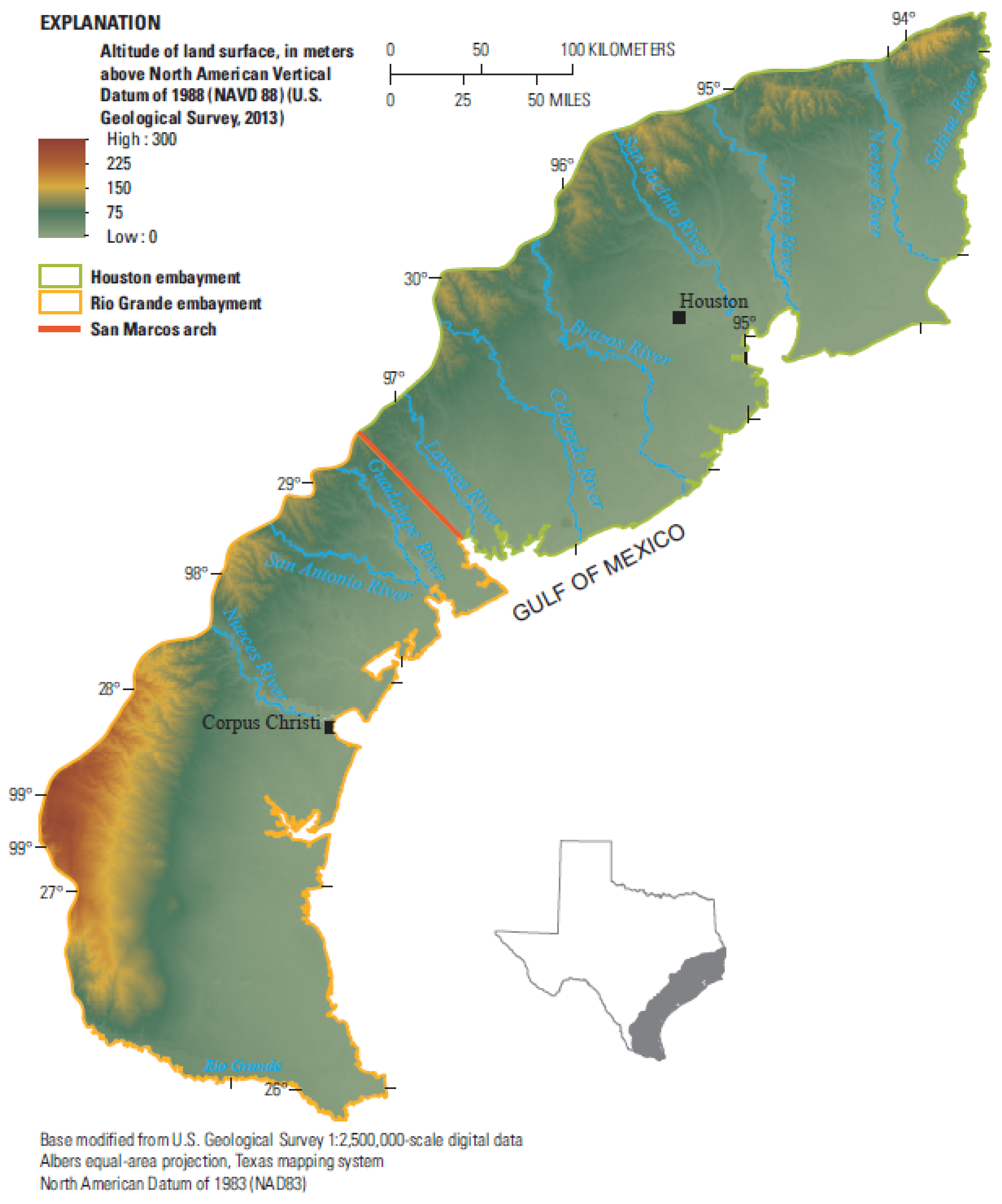
A composite hydrogeologic unit was created by combining geologic and hydrogeologic data and maps for individual geologic and hydrogeologic units. The composite hydrogeologic unit consists of the combination of all hydrogeologic units included in the permissive tract. A review of available data in the permissive tract was done to assess the quantity and quality of data pertaining to the hydrogeologic framework. Data used for the permissive tract were from regional and national datasets so that the applicability of the methodology documented herein can be used in other locations. Furthermore, the most complete and most current datasets were used. Data for each of the hydrogeologic units within the permissive tract were obtained and compiled into composite maps to describe the hydrogeologic framework of the entire permissive tract. A composite hydrogeologic unit is warranted for the geoenvironmental assessment because (1) aquifer units in permissive tract 3 are not separated by confining units or other relatively impermeable units, therefore migration of contaminants originating from any hydrogeologic unit may flow into units below or above the source of contamination and (2) U resources are thought to exist within the permissive tracts; the location of the U resources are unknown because the U resource assessment provided estimates of undiscovered U resources and did not assess the potential locations for these estimated resources. Mapping hydrogeologic information such as composite hydrogeologic unit altitudes and depths, water-level altitudes and depths of water, unsaturated and saturated zone thicknesses, and transmissivity and hydraulic conductivity was carried out as part of the geoenvironmental assessment. Although the resulting surfaces of the hydrogeologic information are displayed in a two-dimensional space for the purpose of presentation, they can be readily depicted in a three-dimensional space for visualization and interpretation.

2.1. Land Surface

A digital elevation model (DEM), the Three-Dimensional Elevation Program dataset (3DEP), was obtained from the National Map [32] for the area containing permissive tract 3 [33]. The 3DEP DEM was converted from geographic coordinates in decimal degrees to Universal Transverse Mercator projected coordinates (zone 14), in meters, with both projections based on the North American Datum of 1983 (NAD 83), using Geosoft’s Oasis montaj software package [34]. The altitude data remained in its native units of meters above the North American Vertical Datum of 1988 (NAVD 88). NAVD 88 is a geodetic datum based on the local mean sea level height value at Father Point in Rimouski, Quebec, Canada. Tidal datums such as mean sea level are used as local vertical references and demonstrate variations in sea surface topography between tidal benchmarks [35]. Because of these variabilities between tidal benchmarks, a fixed refence datum such as NAVD 88 was used. The land-surface altitudes are based on a 10 m cell resolution. Vertical positional accuracy of the DEM is about 3.04 m at a 95% confidence level in terms of the National Standard for Spatial Data Accuracy, but accuracy may vary substantially across the study area because of differences in source information quality, terrain relief, land cover, and other factors [36].

2.2. Composite Hydrogeologic Unit Base and Midpoint

Geologic unit altitude surfaces were obtained from Young et al. [5,6,12] which contained the grid mosaic, or meshing of multiple surface grids into one surface grid, surfaces for the altitudes of the bases for the upper part of the Lagarto Clay, Goliad and Willis Sands, and Lissie and Beaumont Formations; the geologic units that contain the Chicot and Evangeline aquifers. This paper is focused on permissive tract 3, so the base and midpoint are for the composite unit containing the upper part of the Lagarto Clay (as included in the Evangeline aquifer by Young et al. [5,6,12]), Goliad and Willis Sands, and the Lissie and Beaumont Formations, as well as any alluvial sediments [33]. Each geologic unit altitude surface was converted from Albers projected coordinates, in feet, to Universal Transverse Mercator projected coordinates (zone 14), in meters, with both projections based on the NAD 83, using Geosoft’s Oasis montaj software package [34]. The altitude data were converted from feet above NAVD 88 to meters above NAVD 88.
The lowest altitude for each coincident grid cell associated with the raster data defining the altitudes of the bases of the upper part of the Lagarto Clay, Goliad and Willis Sands, and Lissie and Beaumont Formations was selected to create the composite hydrogeologic unit base altitude of permissive tract 3 [33]. A composite hydrogeologic unit midpoint altitude of permissive tract 3 was calculated by taking the average of the land-surface altitude and the composite hydrogeologic unit base altitude surfaces for each grid cell. Hydrogeologic surfaces showing depth of composite hydrogeologic unit base and depth of composite hydrogeologic unit midpoint were calculated by subtracting both the composite hydrogeologic unit base altitude surface and the composite hydrogeologic unit midpoint altitude surface from land-surface altitudes, respectively.

2.3. Compilation and Gridding of Water-Level Altitude Data

Water-level altitude data were compiled, evaluated, and gridded to construct surfaces of water-level altitudes and depths of water below land surface for permissive tract 3. Water-level altitude data compiled from the Texas Water Development Board’s (TWDB) groundwater database (GWDB) [37] were quality checked and used to construct the water-level altitude surface [33]. Because variations in land-surface altitudes can occur in short distances resulting in variable depths across these distances, all measurements of the depths of water in meters below land surface were converted to water-level altitudes in meters above NAVD 88 to account for these variations and to result in a smoother surface during the kriging process. To represent the recent water-level altitudes, only water levels from the ten-year period prior to the start of the study (1 January 2007, to 31 December 2016) were used. The accuracy of each measurement was evaluated based on measurement method, well status such as condition of the well at the time of measurement, and the measurement status such as surrounding conditions (nearby groundwater withdrawals) that could affect the measurement (reported as comments in the dataset) [33]. If the measurement method, well status, or measurement status indicated that a water level was less accurate than what was reported, the measurement value was rounded to a reevaluated accuracy (for example, a change in accuracy could be reduced from centimeters to decimeters). To eliminate bias resulting from multiple measurements made at any individual well, the median value for all measurements at an individual well during the selected ten-year period of record was used. Prior to calculating the median water-level altitude for each well, all suspect data (for example, water levels affected by groundwater withdrawals at or near the well or measurements noted as “questionable” because of spotty tape readings) were excluded. The water-level altitude measurements were separated by aquifer from which the measurement was made, which is identified based on the aquifer code from the well information table in the TWDB database [33,37]. To ensure all variations of aquifer code designations for geologic and hydrogeologic units within the permissive tract were obtained, the first three numbers in the aquifer code were used to aggregate the data. For permissive tract 3, all water-level measurements with aquifer codes having a “112” (typically contained in the Pleistocene-age units) or a “121” (typically contained in Pliocene-age units) numerical designation that were located within the geographic extent of the permissive tract were used to construct the water-level altitude surface.
After the water-level altitudes were compiled and evaluated for quality, a gridded water-level altitude surface [33] was created using kriging interpolation techniques in Oasis montaj [38]. Kriging is a statistical gridding method of interpolation that uses the variance of the dataset to estimate the data values for the cells of the grid [39]. Knowing the cell size and the variogram model, a grid can be created. To determine the grid cell size, the distance to the nearest neighboring data location was found. One-half of the median distance value was used for the grid cell size. A variogram model was created to optimize the kriging results. A variogram is a statistical analysis chart showing variance against distance between each paired point within the selected dataset [39]. Based on the observed data, a model (variogram model) is fitted to best represent the data (Figure 5). This model is then used in the gridding process to estimate the cell values in the grid and to calculate the variance for that cell. Anisotropy, or spatial correlations of the data, may occur within a dataset. Any anisotropy within the selected dataset was identified and accounted for during the kriging process. Seequent [38] contains a complete description of the kriging methods used for grid interpolation.
Preliminary grids were used to identify outliers and areas requiring review. To aid in identifying outliers, the residual was calculated as the difference between the median water-level altitude at each well and the interpolated grid value [40]. All locations with a residual greater than an absolute value of 1.8 m (6 feet (ft)) were evaluated through a correlation process to determine data-point uncertainty. The correlation process involved the comparison of the water-level altitude at a given site to the water-level altitude at nearby sites to determine if it “correlated” with the nearby water-level altitude. If the water-level altitude varied by more than 1.8 m from the nearby water-level altitudes and seemed to not coincide with the overall water-level altitude surface of the area, it was removed from the final grid.
After the initial correlation process was finished, all water-level altitudes were reevaluated based on their necessity, which is dictated by the need to fill any data gaps. The need to fill data gaps is determined by evaluating the standard variance grid created during the gridding process [38]. The standard variance of water-level altitudes indicates the degree to which water-level altitudes in a given area are similar [39,41]. The standard variance grid shows the variance of the gridded water-level altitudes where relatively small variances are typically located near the water-level altitude measurement location and relatively large variances are typically located equidistantly between water-level altitude measurement locations. All locations with a standard variance greater than 1.4 square meters (m2) (15 square feet (ft2)) and a residual less than 9.1 m (30 ft) (to reduce the inclusion of extreme outlying data) were evaluated through the data necessity process to dictate inclusion of the data to fill data gaps. If the water-level altitude was located where the standard variance was greater than 1.4 m2 (15 ft2), differed by less than 9.1 m (30 ft) from the nearby water-level altitudes, and seemed to coincide with the overall water-level altitude surface of the area, it was included in the final grid. Throughout the process, all median water-level altitudes were reviewed and revised as needed to provide a better understanding of the recent (2007–2016) water-level altitudes. The final resulting grids are referred to as the water-level altitude surface and standard variances of the water-level altitude. A grid showing depth of water was calculated by subtracting the water-level altitude surface from land-surface altitude.
Figure 5. Variogram showing the correlation between the variance of all paired data values and the spatial distance between those paired values for the observed (black line in top panel) and simulated (variogram model; red line in top panel) water-level altitude data as well as the number of sampled value pairs compared to distance between paired values (black line in bottom panel). The nugget describes the small-scale variability of the data over short distances [42]. The sill describes the maximum variability between point pairs and the range describes the distance at which point pairs are no longer spatially correlated [41,43].
Minerals 12 00420 g005

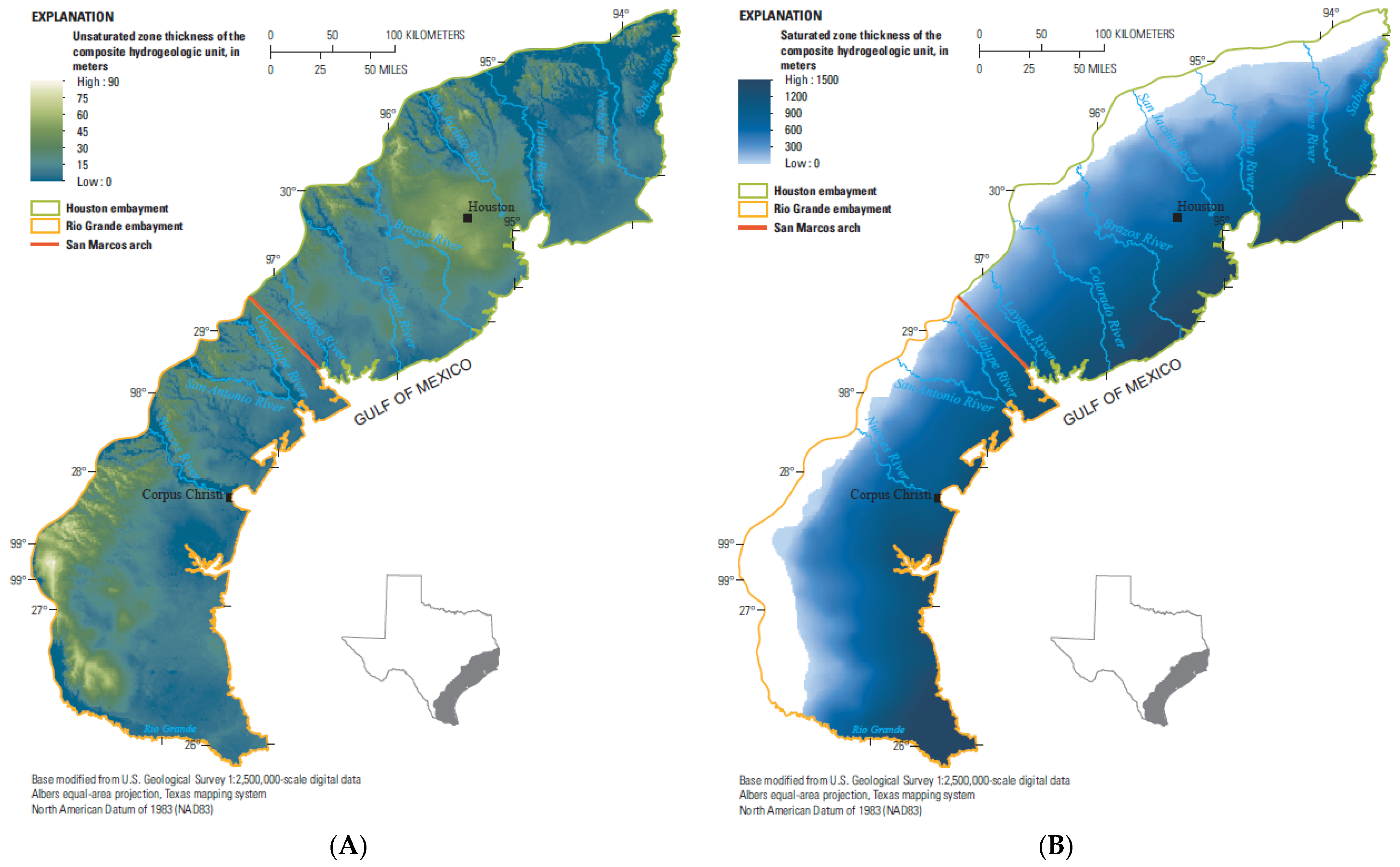
2.4. Unsaturated and Saturated Zone Thickness

Once the water-level altitude surface was created, the unsaturated zone thickness [33] was calculated by subtracting the water-level altitudes from the land-surface altitudes for each grid cell [37]. The difference between the land-surface altitude and the water-level altitude equals the depth of water. Unsaturated zone thickness values of zero were assumed to represent areas where water levels were very near land surface. Conversely, saturated zone thickness [33] was calculated for the permissive tract by subtracting the altitude of the composite hydrogeologic base of the permissive tract from the water-level altitudes for each grid cell [37]. Saturated zone thickness values of zero were assumed to represent dry (unsaturated) geologic conditions (at least for the geologic units within the permissive tract). Furthermore, river drainages within the permissive tract were not evaluated for their connection with the water table nor were the water-surface altitudes in the rivers used during the kriging of the water-level altitudes. Kriging of the water-level altitudes without water-level altitudes available from wells near river drainages to serve as control points may result in water-level altitudes that are higher than land surface. Water-level altitudes near river drainages were adjusted after the kriging process to ensure no water-level altitudes were above land surface.

2.5. Transmissivity and Hydraulic Conductivity

Understanding the hydraulic properties (transmissivity and hydraulic conductivity) of an aquifer is critical to understanding the ability of groundwater to pass through it [44,45,46]. Transmissivity is defined as the rate water is transmitted through a unit thickness of an aquifer under a unit hydraulic gradient (Figure 6). The hydraulic conductivity of an aquifer is the transmissivity divided by the aquifer thickness (or saturated zone thickness if unconfined). Hydraulic conductivity is a measure of the ability of a porous material to allow fluids to pass through it. Higher hydraulic conductivity values correlate with higher yields and less drawdown in a well [45].
The USGS Source Water Assessment Program (SWAP) [47,48] provides a dataset of hydraulic property information for much of the study area. The SWAP dataset was explored to determine if the hydraulic property information that it contains could be applied to the composite aquifer. Raster datasets with 60 m resolution were used to create grids representing the transmissivity (T) and saturated zone thickness (B) of the Chicot and Evangeline aquifers in order to determine transmissivity and hydraulic conductivity for the composite hydrogeologic unit in permissive tract 3.
For each aquifer, hydraulic conductivity (K) was derived by dividing the T grids by the B grids. Then, Equation (1) was used to calculate a single representative K for the composite hydrogeologic unit:
K e q = m = 1 n K m b m b ,
where Keq is the equivalent conductivity, Km is the conductivity for aquifer m, and bm is the thickness for aquifer m. This equation is specifically for horizontal conductivity (parallel, not perpendicular, to areal extent of the aquifer) and assumes each aquifer is homogeneous and that the horizontal hydraulic gradient is the same for both aquifers. Once calculated, the equivalent conductivity was multiplied by the total saturated zone thickness of both aquifers to obtain an equivalent transmissivity.

3. Results

The composite hydrogeologic unit for permissive tract 3 consists of the geologic units that contain the Chicot and Evangeline aquifers. Data pertaining to the geologic units that contain each of the aquifers were compiled into composite maps describing the hydrogeologic framework of the entire permissive tract as part of a geoenvironmental assessment of the undiscovered uranium resources in the upper part of the Lagarto Clay, Goliad and Willis Sands, Lissie and Beaumont Formations, and alluvial sediments in the Texas Coastal Plain [33]. Wherever possible, existing data were used to build the hydrogeologic framework. These data included a land-surface DEM used to determine land-surface altitudes; geologic unit surface altitudes (base and midpoints of the composite hydrogeologic unit); and the water-level measurements used to determine water-level altitudes and the locations of unsaturated and saturated zones [33]. In addition, the amount and spatial coverage of the existing data was sufficient to determine transmissivity within most of permissive tract 3.

3.1. Topographic Features

The topography of permissive tract 3 is characterized by flat low-lying expanses dissected by relatively slow-moving rivers throughout most of the Texas Coastal Plain; higher terrain characterized by steeper topographic features are found along the edges of the permissive tract to the north and west (Figure 7). Compared to flat low-lying terrain, higher terrain with relatively steep topographic features can often lead to differences in the depths of hydrogeologic units and depths of water. Land-surface altitudes in the Houston embayment range from 185 m above NAVD 88 in some areas in the uplands in the north to 0 m above NAVD 88 in the coastal regions; altitudes less than 90 m above NAVD 88 are common in most (about 90 percent) of the Houston embayment (Figure 7) [33]. The overall topography of the Rio Grande embayment is steeper than the topography of Houston embayment (Figure 7). Most of the Rio Grande embayment (about 90 percent) is less than 150 m above NAVD 88; exceptions are mostly found in the western part of the embayment where the land surface is as high as 288 m above NAVD 88 (Figure 7) [33]. Compared to the Houston embayment, river drainages are less prominent topographic features in the Rio Grande embayment, reflecting the increasingly arid environment moving from east to west across the study area [49,50]. There are no large river drainages in the southern and southwestern parts of the Rio Grande embayment except for the Rio Grande; several large river drainages (Guadalupe, San Antonio, and Nueces Rivers) are in the eastern part of the Rio Grande embayment southwest of the San Marcos arch (Figure 7).

3.2. Analysis of Composite Hydrogeologic Unit Base and Midpoint

The depths of the base of the composite hydrogeologic unit of permissive tract 3 are similar between the two embayments (Figure 8A). Depths of the base of the composite hydrogeologic unit range from 0 m at land surface (outcrop areas) to 1804 m below land surface in the Houston embayment and 2799 m below land surface in the Rio Grande embayment with an exceptionally deep area in the southeastern part of the embayment (Figure 8A) [33]. As a result of the coastward dip of the hydrogeologic units in the Texas Coastal Plain, the base of the composite hydrogeologic unit becomes progressively deeper towards the Gulf of Mexico. Throughout most of permissive tract 3 (about 90 percent), the depths of the base of the composite hydrogeologic unit are less than 1300 m below land surface (Figure 8A) [33].
Because depths pertaining to the composite hydrogeologic unit are referenced to land surface, and the top of the composite hydrogeologic unit is equivalent to the land surface, the depths of the midpoint of the composite hydrogeologic unit are essentially one-half of the depths of the base of the composite hydrogeologic unit. For these same reasons, the midpoint altitudes of the composite hydrogeologic unit trend in a similar way compared to the base altitudes of the composite hydrogeologic unit. Depths of the midpoint of the composite hydrogeologic unit range from 0 m at land surface (outcrop areas) to 902 m below land surface in the Houston embayment and 1400 m below land surface in the Rio Grande embayment with a deep area in the southeast part of the embayment (Figure 8B) [33]. Throughout most of permissive tract 3 (about 90 percent), the depths of the midpoint of the composite hydrogeologic unit are less than 650 m below land surface (Figure 8B) [33].
The base and midpoint altitudes of the composite hydrogeologic unit exhibit similar trends to those in the depths of the base and midpoint of the composite hydrogeologic unit. Therefore, a description of the base and midpoint altitudes of the composite hydrogeologic unit is not necessary. The base and midpoint altitudes of the composite hydrogeologic unit are available in the companion data release [33] for applications needing altitude data.

3.3. Analysis of Water-Level Altitudes and Depth of Water

The standard variance of water-level altitudes ranged from 0.0 to 8.5 m2 in permissive tract 3 (Figure 9) [33]. The standard variance was minimal in most of the Houston embayment, ranging from 0.0 to 3.0 m2. The standard variance was generally the highest along the edges of permissive tract 3, especially in the extreme southeastern part of the Houston embayment. The standard variance of the water-level altitudes in the Rio Grande embayment ranged from 0.0 to 6.8 m2 (Figure 9) [33]. The standard variance increased towards the southwestern part of the Rio Grande embayment and ranged from 3.1 to 6.0 m2 in many parts of this embayment. The standard variance exceeded 6.0 m2 along the edges of permissive tract 3 within the Rio Grande embayment. Large standard variance values (greater than 4.5 m2) were indicated for water-level altitudes in the southern part of permissive tract 3, an area where water-level altitude data are scant. Because of the scant amount of available data and the large grid variance in this area and along the edges of permissive tract 3, the water-level altitude surface produced for the southern part of permissive tract 3 may not represent recent (2007–2016) water-level altitudes.
For permissive tract 3, there were 970 wells used in the final water-level altitude surface (Figure 10A) [33]. As with the land-surface altitudes, water-level altitudes tend to be higher along the northern and northwestern margins of the permissive tract. Water-level altitudes in the Houston embayment ranged from 124 m above NAVD 88 in some areas in the uplands to the north to −40 m above NAVD 88 in the coastal regions (Figure 10A) [33]. A prominent feature in the water-level altitude surface is an area of low water-level altitudes, or cone of depression, that is evident in the greater Houston area where major groundwater withdrawals have occurred; this area also has undergone land-surface subsidence [51]. Major river drainages are identified in both embayments based on water-level altitudes except in the greater Houston area, where the cone of depression overshadows the major river drainage (Figure 10A). Based on water-level altitudes, horizontal hydraulic gradients in the Rio Grande embayment are steeper than the Houston embayment, especially in the western part of permissive tract 3 (Figure 10A). Water-level altitudes in the Rio Grande embayment range from 225 to −11 m above NAVD 88, with most of the embayment (about 90 percent) having water-level altitudes less than 120 m above NAVD 88 (Figure 10A) [33]. River drainages are less prominent in the Rio Grande embayment to the south, mainly because of a more arid environment in the south and southwest [49,50]. Several river drainages are prominent southwest of the San Marcos arch (Figure 10A).
The depth of water within the Houston embayment ranges from land surface to 76 m below land surface (Figure 10B) [33]. The northeastern third of the Houston embayment (east of the Trinity River) includes large areas with shallow groundwater depths ranging from 0 to 15 m below land surface (Figure 10B). The cone of depression in the greater Houston area noted previously is reflected by deeper depths of water than the surrounding areas because of large groundwater withdrawals [51]. Prominent river drainages are easily identified in the depth of water map (Figure 10B). The depths of water within the Rio Grande embayment range from land surface to 90 m below land surface (Figure 10B) [33]. Throughout most of the Rio Grande embayment (about 90 percent), depths of water are less than 40 m below land surface (Figure 10B) [33]. Several river drainages are prominent southwest of the San Marcos arch (Figure 10B). In addition, there are several areas in the southwestern and western parts of the Rio Grande embayment where the groundwater is relatively deep. Compared to other parts of permissive tract 3, the depth of water tends to be larger in this part of permissive tract 3 where the climate is arid and the terrain is relatively steep [49,50].

3.4. Analysis of Unsaturated and Saturated Zone Thickness

For most of permissive tract 3, the water table is relatively near the land surface, resulting in relatively thin unsaturated zone thicknesses of the composite hydrogeologic unit in permissive tract 3. The unsaturated zone thicknesses of the composite hydrogeologic unit range from 0 (or completely saturated) to 90 m within the Houston embayment, but the unsaturated zone thicknesses of the composite hydrogeologic unit throughout most of the embayment (about 90 percent) are less than 40 m (Figure 11A) [33]. The unsaturated zone thickness of the composite hydrogeologic unit is greater than 40 m in the greater Houston area, reflecting the large groundwater withdrawals and resultant lower water-level altitudes described previously (Figure 10A). The unsaturated zone thicknesses of the composite hydrogeologic unit are generally smallest northeast of Houston near the edge of the permissive tract, a region that typically receives more precipitation (average annual precipitation ranges between 150 and 180 cm (cm), annually) and has a smaller population and thus less groundwater demand [50]. The unsaturated zone thicknesses of the composite hydrogeologic unit within the Rio Grande embayment range from zero (complete saturation) to 90 m, but the unsaturated zone thicknesses of the composite hydrogeologic unit throughout most of the embayment (about 90 percent) are less than 40 m, which is greater than the unsaturated zone thicknesses of the composite hydrogeologic unit in the Houston embayment (Figure 11A) [33]. The southwestern part of permissive tract 3 is very arid (average annual precipitation ranges between 40 and 60 cm, annually), so less water is available for potential recharge [50]. Prominent river drainages, which are potential sources of recharge to underlying aquifers, can be seen in Figure 11.
For permissive tract 3, the saturated zone thicknesses of the composite hydrogeologic unit in permissive tract 3 are typically lower on the northern and western extent of the permissive tract with thicknesses increasing to the southeast towards the Gulf of Mexico (Figure 11B). The thickest area of saturation is in the southeastern tip of permissive tract 3. The saturated zone thicknesses of the composite hydrogeologic unit of permissive tract 3 range from no saturation to 1794 m within the Houston embayment, with most of the saturated zone thicknesses of the composite hydrogeologic unit (about 90 percent) being less than 1300 m thick (Figure 11B) [33]. The saturated zone thicknesses of the composite hydrogeologic unit range from no saturation to 2786 m within the Rio Grande embayment; however, most of the Rio Grande embayment saturated zone thicknesses of the composite hydrogeologic unit (about 90 percent) are less than 1200 m, which is less than that which occurs in the Houston embayment (Figure 11B) [33].

3.5. Analysis of Transmissivity and Hydraulic Conductivity

The SWAP dataset described previously in the Transmissivity and Hydraulic Conductivity section of the Material and Methods section did not cover all permissive tract 3 (Figure 12). Consequently, historical transmissivity, hydraulic conductivity, and storativity values from previous studies were compiled and used to supplement the SWAP dataset (Table 1). Porosity values for the Texas Coastal Plain are not widely reported, but Young et al. [12] reported porosity results ranging between 20 and 45 percent. This porosity range was reported from multiple geophysical logs measured in wells completed in aquifers above the Catahoula Formation (Chicot, Evangeline, and Jasper aquifers). Young et al. [12] observed a gradual decrease (0.0033 percent per meter) in porosity with depth despite the considerable amount of scatter in the porosity results. They estimate that average porosity values near land surface are around 36.64 percent [12]. Using this average porosity at land surface, the observed porosity gradient with depth, and the depth of the base of the composite geologic unit, the average porosity ranges between 30.72 and 36.64 percent within the composite hydrogeologic framework. The storativity and porosity values are presented herein as supplemental data that can be used to estimate the volume of water in the aquifer using the saturated thickness in a given area. The hydraulic gradient as determined from changes in water-level altitude, transmissivity or hydraulic conductivity, the storativity, and porosity are useful aquifer characteristics to estimate contaminant transport. The storativity and porosity values are not further evaluated or interpreted in this paper.
Transmissivity values in the Houston embayment are between 0 and 4181 square meters per day (m2/d), but throughout most of the embayment (about 90 percent), transmissivity values are less than 1800 m2/d (Figure 12A). A prominent area characterized by large transmissivity values is present southwest of Houston. In terms of available transmissivity values, the Rio Grande embayment has less spatial coverage than the Houston embayment (Figure 12A). In areas where data are available, transmissivity values tend to be smaller than the transmissivity values in the Houston embayment. Transmissivity values in the Rio Grande embayment range from 0 to 1871 m2/d, but throughout most of the embayment (about 90 percent), transmissivity values are less than 1500 m2/d (Figure 12A).
Hydraulic conductivity values in the Houston embayment are between 0 and 15 m per day (m/d) (Figure 12B), but throughout most of the embayment (about 90 percent), hydraulic conductivity values are less than 7 m/d. As with the transmissivity data, there is a prominent area characterized by large hydraulic conductivity values southwest of Houston. Similarly, and as with the extent of available transmissivity values, the Rio Grande embayment has less spatial coverage than the Houston embayment, and the available hydraulic conductivity values in the Rio Grande embayment tend to be smaller than the hydraulic conductivity values in the Houston embayment (Figure 12B). Hydraulic conductivity values in the Rio Grande embayment range from 0 to 9 m/d (Figure 12B), but throughout most of the embayment (about 90 percent), hydraulic conductivity values are less than 7 m/d.

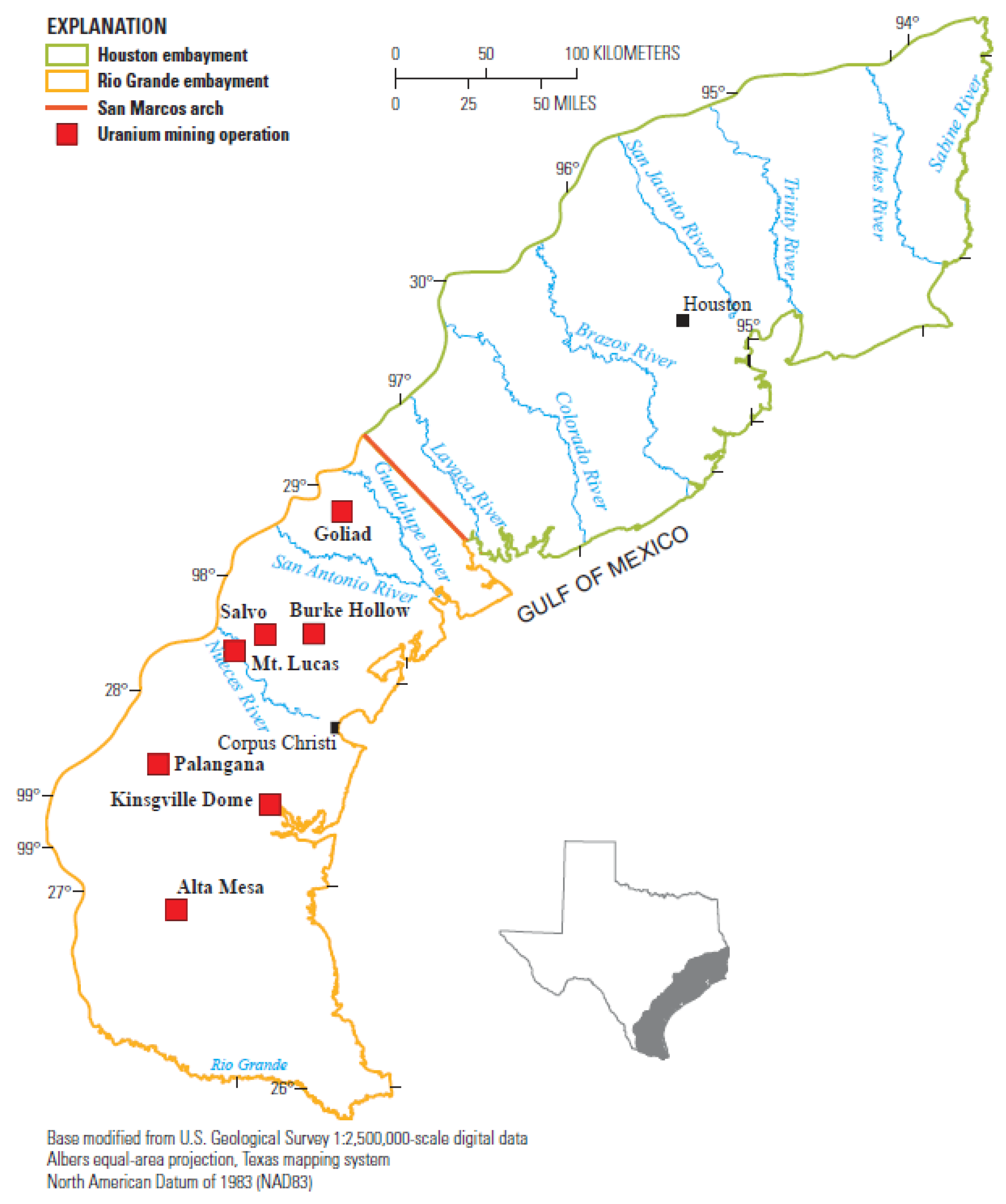
3.6. Comparison of the Hydrogeologic Framework to Technical Reports

To help evaluate the potential usefulness of the hydrogeologic framework to future U mining geoenvironmental assessments, key results from the hydrogeologic framework were compared to historical technical reports at selected U mining operations in permissive tract 3 (Figure 13, Table 2) [62,63,64,65,66,67,68,69,70,71,72]. The location of the U mining operation and the topography at the site were noted. The technical reports were reviewed for data pertaining to geologic unit thickness or depth that can be used to approximate the depth of the composite hydrogeologic unit at the operation. Any data pertaining to the depth of water were noted as well. Comparison of transmissivity and hydraulic conductivity values between the hydrogeologic framework and historical technical reports was not carried out because these data were scant for the Rio Grande embayment within the hydrogeologic framework and the technical reports rarely reported transmissivity and hydraulic conductivity values. One reported transmissivity value (404 m2/d) was at the Mt. Lucas operation [69] which corresponds closely to the nearest transmissivity values (about 200–300 m2/d) (Figure 12A). All data obtained were approximated for the area of mining operation, which often encompassed several square kilometers. Large variations of topography, base to geologic unit, and depth of water can occur within areas of this size. In all of the technical reports, the bases of geologic units were not verified with the well data. Typically, regional geologic assessments were used to estimate the depths of formations at the operation. There were accurate well data for the individual sand layers containing the U deposits, but all of the well data did not penetrate the base of the Goliad Sand.
Even though the altitudes in the technical reports were reported in mean sea level and the altitudes in this paper are in NAVD 88, there is little difference (less than 10 percent) between the approximated land-surface altitudes from the technical reports and the estimated land-surface altitudes from the hydrogeologic framework (Table 2). Some of this variation can be attributed to the different vertical datums. Another contributing factor could be because of large variations of altitude at the mining operation. Altitude changes of as much as 27 m were observed at some mining operations such as at the Palangana mining operation (Figure 13) [70,71].
There were notable differences between the approximated depth of the base of the composite hydrogeologic unit from the technical reports and the estimated depth of the base of the composite hydrogeologic unit from the hydrogeologic framework (Table 2). These large differences can be a result of multiple factors. The geologic information obtained from the technical reports was already a generalized description of the formations at the operation and the geologic information was not verified with well data (at least not to the base of the Goliad Sand). Furthermore, the composite hydrogeologic unit in this paper includes the sandy upper part of the Lagarto Clay, which may not have been included as part of the Goliad Sand in the geologic setting of the technical reports. As a result, the composite hydrogeologic unit in this paper should be deeper than the composite hydrogeologic unit in the technical reports, and this was consistently the case except at the Alta Mesa mining operation (Figure 13, Table 2). Given that there were expected differences between the approximate depth of the base of the composite hydrogeologic unit from the technical reports and the estimated depth of the base of the composite hydrogeologic unit from the hydrogeologic framework, the differences were relatively small (the percent differences were less than 70 percent at most of the mining operations) (Table 2).
The approximate depth of water from the technical reports and the estimated depth of water from the hydrogeologic framework were relatively similar with differences of 10 m or less except at Kingsville Dome mining operation, where the difference was 24 m (Figure 13, Table 2). The large difference at Kingsville Dome is a result of the limitations of the hydrogeologic framework. Kingsville Dome is next to a bay southwest of Corpus Christi (Figure 13). As stated in the “Analysis of Water-Level Altitudes and Depth of Water” section of this paper, the amount of available data is scant for this part of Texas, which resulted in large grid variances (Figure 9) in the area and estimated water-level altitudes that may not represent recent (2007–2016) water-level altitudes. As stated in the “Analysis of Unsaturated and Saturated Zone Thickness” section of this paper, river drainages were not evaluated for their connection with the water table nor were the water-surface altitudes in the rivers used during the kriging of the water-level altitudes. Because the Kingsville Dome mining operation is near a bay (Figure 13), the same principle applies in that water-surface altitudes for groundwater under the bay were not available for use during the kriging of the water-level altitudes. Because of the scant data in the area and because of the proximity of Kingsville Dome to the bay, large differences are seen between the approximate depth of water from the technical report and the estimated depth of water from the hydrogeologic framework. The variations seen in the other operations can be a result of the dates at which the depth of water was measured. The more recent (2007–2016) technical reports [62,65,66] have closer results than the older (1981–1985) technical reports [67,68,69], which is expected because water-level altitudes are in constant flux and the depth of water surface in this paper was from recent (2007–2016) water-level measurements.

4. Discussion

A hydrogeologic framework for the study area was developed to gain a better understanding of the potential effects of mining undiscovered uranium resources in the study area by using available data from regional and national datasets; a similar approach could be applied to other areas of undiscovered mineral resources. Large-scale regional datasets can be evaluated as a first step, such as the hydrogeologic units and water-level measurements compiled for this study. Many areas have historical hydrogeologic information available, including data in the preferred form of grid surfaces [5,6,12,17,37]. For this study, data obtained from water-level measurements were used to obtain water-level altitude and depth of water surfaces [33,37]. Water-level measurements are typically reported to State and Federal agencies and readily available. When large-scale regional datasets were not available or were lacking sufficient spatial data for the study area evaluated herein (permissive tract 3), national datasets were used such as the land-surface DEM and SWAP data for this study [32,47,48]. The land-surface DEM from the 3DEP is a mosaic grid of the best resolution data for the compiled area [32]. This can range from 1 m to 60 m of resolution but is typically 10 m resolution. The SWAP dataset, which is a large national dataset, was used to help supply aquifer hydraulic properties, but the lack of sufficient areal coverage for the study area meant that this dataset needed to be supplemented with other data to fill in data gaps [47,48]. The saturated thickness surfaces with estimated hydraulic conductivity values could be used in place of a transmissivity surface.
The relative abundance and diversity of the available data for the Chicot and Evangeline aquifers of the Texas Coastal Plain [5,6,12,17,32,37,47,48] made the development of the hydrogeologic framework of a composite hydrogeologic unit for permissive tract 3 possible without the need to collect additional data; the data available for other areas may not be as abundant or diversified. Whereas regional and national datasets facilitated the development of hydrogeologic frameworks describing composite hydrogeologic units, such datasets may be lacking in other areas. If a hydrogeologic framework is to be developed using the methods documented herein for other areas, evaluating the available datasets would be a useful first step. Documenting the limitations of compiled datasets aids in assessing the resolution of the final hydrogeologic framework. When the existing data are deemed inadequate, additional data may need to be collected.
As inherent with all assessments, there are limitations and assumptions that apply to the data compiled for this assessment. The resolution of the DEM will dictate the resolution for each layer calculated by using land-surface altitudes. There were varying degrees of horizontal resolution associated with each dataset ranging from 10 to 1250 m in the land-surface altitude and water-level altitude surfaces, respectively [32,33]. When a dataset was evaluated on an individual basis, its original resolution was retained, but when multiple datasets were compared or interpreted together, the dataset with the lowest resolution was used to dictate the resolution of the composite dataset. The geologic unit surfaces were interpreted to represent the “true” geology, but interpretation techniques may differ between geologists [5,6,7,8,9,10,11]. The aquifers from which water-level measurements were obtained for this study were assumed to be correctly identified, the well locations were assumed to be correct, and the water-level measurements were assumed to be attributed correctly in terms of the accuracy of the measurement and the potential for interference from nearby groundwater withdrawals [37]. Although the kriging technique is based on geostatistical interpolation [38,39], the resulting gridded data can be spatially distal from actual water-level measurements. Because the areas between actual measurements lack constraint, the water level may be higher or lower than that which is depicted. The spatial separation between gridded and actual water-level measurements initially resulted in some negative depth of water values that needed to be corrected when constructing the unsaturated zone thickness map, especially in river drainage areas. All negative depth of water (unsaturated zone thickness) values were adjusted to be 0 m. The transmissivity and hydraulic conductivity data are scant for permissive tract 3, especially in the Rio Grande embayment [47,48]. All interpretations presented in this paper represent a regional-scale approximation and, as such, are not intended for use in local or small-scale engineering or other design applications. Users evaluating the findings provided in this paper should exercise discretion when drawing conclusions or making policy decisions.
The hydrogeologic framework consists of the lithology, hydrostratigraphy, structural features, and hydraulic properties of one or multiple hydrogeologic units. Although this paper discussed the methods of developing a hydrogeologic framework for a composite hydrogeologic unit, a similar methodology can be applied to a singular hydrogeologic unit. Effectively, the purpose of combining multiple hydrogeologic units is to simplify the hydrogeology into a singular composite hydrogeologic unit to effortlessly include hydrogeologic framework interpretations into a geoenvironmental assessment.
For the purpose of in situ uranium recovery, confining units are typically required to reduce the potential for hydraulic connection between aquifers [4]. Although none of the individual geologic units composing the composite hydrogeologic unit constructed for this study are considered confining units (except possibly the Beaumont Formation), extensive clay lenses in each unit may locally act as confining units. Furthermore, the Evangeline aquifer is considered by some researchers to be a confined unit in the sense that it has a different hydraulic head compared to the overlying Chicot aquifer, most likely a result of multiple interbedded clays [73], although, as previously mentioned, migration of contaminants originating from any formation may flow into units below or above the source of contamination.

5. Conclusions

The composite hydrogeologic framework presented herein, which contains the Chicot and Evangeline aquifers of the Gulf Coast aquifer system, provides three-dimensional insights into the land-surface altitudes, composite hydrogeologic unit altitudes and depths, water-level altitudes and depths, unsaturated and saturated zone thicknesses, and transmissivity and hydraulic conductivity in a region with the potential for undiscovered uranium resources. Although the original hydrogeologic data and maps are informative for each individual geologic and hydrogeologic units [5,6,12,17,32,37,47,48], combining these data to create a depiction of a composite hydrogeologic unit, as presented here, could inform the potential for the migration of contaminants through various avenues. Maps associated with the composite hydrogeologic unit are intended for inclusion in a regional-scale geoenvironmental assessment of undiscovered uranium resources where locations are unknown. Potential applications include using the hydrogeologic framework as an input into a geoenvironmental assessment to help estimate the potential for (1) runoff of contaminants into surface water, (2) infiltration of contaminants into the groundwater (aquifers), or (3) movement of contaminants from the mining area through wind, groundwater-flow, or streamflow in each permissive tract. Land-surface altitudes can be used to identify drainages and depressions which could indicate potential runoff-flow paths. The water-level altitudes and depths of water can be used to identify locations where the water table is shallow; depending on local recharge rates, areas where the water table is shallow could coincide with areas of rapid infiltration of surface water (including runoff) into the soils and rapid groundwater recharge. Composite hydrogeologic unit properties such as land-surface altitude, water-level altitude, depth of water, saturated zone thickness, transmissivity, and hydraulic conductivity provide physical indicators of the potential for the transport of contaminants. The water-level altitudes can also be used to identify groundwater-flow paths, which when coupled with other types of data such as transmissivity values, saturated zone thickness values, and hydraulic conductivity values, would make it possible to estimate the direction and rate of the groundwater flow. The procedures outlined in this paper also provide a method for developing hydrogeologic frameworks that can be applied in other areas where mining may occur.

Author Contributions

Conceptualization, A.P.T. and T.J.G.; methodology, A.P.T.; validation, A.P.T., K.D.B., K.W.-D., D.G.H. and T.J.G.; formal analysis, A.P.T. and D.G.H.; investigation, A.P.T. and D.G.H.; resources, A.P.T. and D.G.H.; data curation, A.P.T. and D.G.H.; writing—original draft preparation, A.P.T., K.D.B. and D.G.H.; writing—review and editing, A.P.T., K.D.B., K.W-D., D.G.H. and T.J.G.; visualization, A.P.T.; supervision, K.W.-D. and T.J.G.; project administration, A.P.T., K.D.B. and K.W.-D.; funding acquisition, K.W.-D. All authors have read and agreed to the published version of the manuscript.

Funding

This work was funded by the U.S. Geological Survey for the Environmental Health Program in the Ecosystems Mission Area.

Data Availability Statement

This product has been peer reviewed and approved for publication consistent with U.S. Geological Survey Fundamental Science Practices (https://pubs.usgs.gov/circ/1367/ accessed on 24 March 2022). Any use of trade, firm, or product names is for descriptive purposes only and does not imply endorsement by the U.S. Government. Writings prepared by U.S. Government employees as part of their official duties, including this paper, cannot be copyrighted and are in the public domain. The grid surfaces of the land-surface altitude, composite hydrogeologic unit base and midpoint altitude and depth, water-level altitude and depth of water, and unsaturated and saturated zone thickness are available online: https://doi.org/10.5066/P9AZMEU0 (accessed on 26 March 2022) [33]. The transmissivity data are published and publicly available, as cited in the manuscript.

Conflicts of Interest

The authors declare no conflict of interest. The funders had no role in the design of the study; in the collection, analyses, or interpretation of data; in the writing of the manuscript, or in the decision to publish the results.

References

  1. U.S. Geological Survey Assessment Team. Assessment of Undiscovered Sandstone-Hosted Uranium Resources in the Texas Coastal Plain, 2015: U.S. Geological Survey Fact Sheet 2015–3069; U.S. Geological Survey: Reston, VA, USA, 2015; p. 4. [CrossRef] [Green Version]
  2. Hall, S.M.; Mihalasky, M.J.; Tureck, K.R.; Hammarstrom, J.M.; Hannon, M.T. Genetic and Grade and Tonnage Models for Sandstone-Hosted Roll-Type Uranium Deposits, Texas Coastal Plains. Ore Geol. Rev. 2017, 80, 716–753. Available online: http://www.sciencedirect.com/science/article/pii/S016913681530038X (accessed on 1 March 2022). [CrossRef]
  3. Weinzapfel, A. Guidebook—Texas Uranium Belt; South Texas Geological Society: San Antonio, TX, USA, 1981; p. 16. [Google Scholar]
  4. International Atomic Energy Agency. In situ Leach Uranium Mining—An Overview of Operations; Series No. NF–T–1.4; International Atomic Energy Agency Nuclear Energy: Vienna, Austria, 2016; p. 60. Available online: https://www-pub.iaea.org/MTCD/Publications/PDF/P1741_web.pdf (accessed on 9 March 2022).
  5. Young, S.C.; Budge, T.; Knox, P.; Kalbouss, R.; Baker, E.; Hamlin, S.; Galloway, B.; Deeds, N. Final Report—Hydrostratigraphy of the Gulf Coast Aquifer System from the Brazos River to the Rio Grande: Prepared for the Texas Water Development Board. 2010; 203p. Available online: https://www.twdb.texas.gov/publications/reports/contracted_reports/doc/0804830795_Gulf_coast_hydrostratigraphy_wcover.pdf (accessed on 1 March 2022).
  6. Young, S.C.; Ewing, T.; Hamlin, S.; Baker, E.; Lupton, D. Final Report—Updating the Hydrogeologic Framework for the Northern Portion of the Gulf Coast Aquifer System: Prepared for the Texas Water Development Board. 2012; 285p. Available online: https://www.twdb.texas.gov/publications/reports/contracted_reports/doc/1004831113_GulfCoast.pdf (accessed on 1 March 2022).
  7. Baker, E.T., Jr. Stratigraphic and Hydrogeologic Framework of Part of the Coastal Plain of Texas: Texas Department of Water Resources Report 236. 1979; 43p. Available online: https://www.twdb.texas.gov/publications/reports/numbered_reports/doc/R236/R236.pdf (accessed on 1 March 2022).
  8. Eargle, D.H. Nomenclature of Formations of Claiborne Group, Middle Eocene, Coastal Plain of Texas, in Contributions to General Geology, 1967: U.S. Geological Survey Bulletin, 1251-D; U.S. Geological Survey: Reston, VA, USA, 1968; 25p. [CrossRef]
  9. Solis, R.F. Upper Tertiary and Quaternary Depositional Systems, Central Coastal Plain, Texas–Regional Geology of the Coastal Aquifer and Potential Liquid-Waste Repositories; The University of Texas at Austin, Bureau of Economic Geology: Austin, TX, USA, 1981; 89p. [Google Scholar]
  10. George, P.G.; Mace, R.E.; Petrossian, R. Aquifers of Texas: Texas Water Development Board Report 380. 2011; 182p. Available online: https://www.twdb.texas.gov/publications/reports/numbered_reports/doc/R380_AquifersofTexas.pdf (accessed on 1 March 2022).
  11. Ryder, P.D. Ground Water atlas of the United States: Segment 4, Oklahoma, Texas, U.S. Geological Survey Hydrologic Atlas 730–E; U.S. Geological Survey: Reston, VA, USA, 1996; 30p. [CrossRef]
  12. Young, S.C.; Jigmond, M.; Deeds, N.; Blainey, J.; Ewing, T.E.; Banerj, D. Final Report—Identification of Potential Brackish Groundwater Production Area—Gulf Coast Aquifer System: Prepared for the Texas Water Development Board. 2016; 636p. Available online: https://www.twdb.texas.gov/publications/reports/contracted_reports/doc/1600011947_InteraGulf_Coast_Brackish.pdf?d=12869.600000023842 (accessed on 1 March 2022).
  13. U.S. Geological Survey. Principle Aquifers of the 48 Conterminous United States, Hawaii, Puerto Rico, and the U.S. Virgin Islands, Version 1.0, U.S. Geological Survey Digital Data; U.S. Geological Survey: Reston, VA, USA, 2003. [CrossRef]
  14. Schruben, P.G.; Arndt, R.E.; Bawiec, W.J.; Ambroziak, R.A. Geology of the Conterminous United States at 1:2,500,000 Scale; A Digital Representation of the 1974 P.B. King and H.M. Beikman Map: U.S. Geological Survey Digital Data Series DDS-11. 1994. Available online: http://pubs.usgs.gov/dds/dds11/ (accessed on 1 March 2022).
  15. Dahlkamp, F.J. Chapter 8 Texas Coastal Plain Uranium Region. In Uranium Deposits of the World, USA and Latin America; Springer: Berlin, Germany, 2010; Volume 2, pp. 311–355. [Google Scholar]
  16. Adams, S.S.; Smith, R.B. Geology and Recognition Criteria for Sandstone Uranium Deposits in Mixed Fluvial-Shallow Marine Sedimentary Sequences, South Texas: Grand Junction, Colorado, U.S. Department of Energy, Report GJBX–4(81); NURE Program; U.S. Department of Energy: Washington, DC, USA, 1981; 154p. [CrossRef] [Green Version]
  17. Young, S.C.; Draper, C. The Delineation of the Burkeville Confining Unit and the Base of the Chicot Aquifer to Support the Development of the Gulf 2023 Groundwater Model: INTERA Incorporated, Prepared for the Harris-Galveston Subsidence District and the Fort Bend Subsidence District. 2020; 75p. Available online: https://hgsubsidence.org/wp-content/uploads/2021/06/Final_HGSD_FBSD_Burkeville_Report_final.pdf (accessed on 1 March 2022).
  18. Campbell, K.M.; Gallegos, T.J.; Landa, E.R. Biogeochemical Aspects of uranium mineralization, mining, milling, and remediation. Appl. Geochem. 2015, 57, 206–235. [Google Scholar] [CrossRef] [Green Version]
  19. U.S. Geological Survey. Geologic Database of Texas, Reston, Virginia. 2014. Available online: https://txpub.usgs.gov/txgeology/ (accessed on 1 March 2022).
  20. Morton, R.A.; Jirik, L.A.; Galloway, W.E. Middle-Upper Miocene Depositional Sequences of the Texas Coastal Plain and Continental Shelf: Geologic Framework, Sedimentary Facies, and Hydrocarbon Plays, The University of Texas at Austin, Bureau of Economic Geology Report of Investigations 174; The University of Texas at Austin, Bureau of Economic Geology: Austin, TX, USA, 1988; 40p. [Google Scholar]
  21. Galloway, W.E. Genetic stratigraphic sequences in basin analysis II: Application to northeast Gulf of Mexico Cenozoic basin. Am. Assoc. Pet. Geol. Bull. 1989, 73, 143–154. [Google Scholar]
  22. Doering, J.A. Post-Fleming surface formations of southeast Texas and south Louisiana. Am. Assoc. Pet. Geol. Bull. 1935, 40, 1816–1862. [Google Scholar]
  23. Plummer, F.B. Cenozoic Systems in Texas: Geology of Texas. Stratigr. Univ. Tex. Bull. 1933, 3232, 519–818. [Google Scholar]
  24. Chowdhury, A.H.; Turco, M.J. Chapter 2 Geology of the Gulf Coast Aquifer, Texas: Texas Water Development Board Report 365, Aquifers of the Gulf Coast of Texas. 2006; 312p. Available online: https://www.twdb.texas.gov/publications/reports/numbered_reports/doc/R365/ch02-Geology.pdf (accessed on 1 March 2022).
  25. Knox, P.R.; Young, S.C.; Galloway, W.E.; Baker, E.T., Jr.; Budge, T. A stratigraphic approach to Chicot and Evangeline aquifer boundaries, central Texas Gulf Coast: Gulf Coast. Assoc. Geol. Soc. Trans. 2006, 56, 371–393. [Google Scholar]
  26. Dubar, J.R.; Ewing, T.E.; Lundelius, E.L., Jr.; Otovs, E.G.; Winker, C.D. Quaternary Geology of the Gulf of Mexico Coastal Plain. In Quaternary Non-Glacial Geology of the Conterminous Unites States; The Geological Society of America: Boulder, CO, USA, 1991; Volume 2, pp. 583–610. [Google Scholar] [CrossRef]
  27. Barnes, V.E. Geologic Map of Texas: Bureau of Economic Geology, The University of Texas at Austin, 4 Sheets, Scale 1:500,000; Bureau of Economic Geology, The University of Texas at Austin: Austin, TX, USA, 1992. [Google Scholar]
  28. Dutton, A.R.; Richter, B.C. Regional Geohydrology of the Gulf Coast Aquifer in Matagorda and Wharton Counties, Texas—Development of a Numerical Model to Estimate the Impact of Water-Management Strategies: Contract Report Prepared for Lower Colorado River Authority, Austin Texas, under Contract IAC (88–89) 0910. 1990; 116p. Available online: https://www.beg.utexas.edu/files/publications/cr/CR1990-DuttonA-1-QAe5623.pdf (accessed on 1 March 2022).
  29. Price, W.A. Sedimentology and Quaternary geomorphology of south Texas. Supplementary to Field Trip Manual—Sedimentology of south Texas, Corpus Christi Geological Society Spring Field Trip. Gulf Coast Assoc. Geol. Soc. Trans. 1958, 8, 41–75. [Google Scholar]
  30. Wood, L.A.; Gabrysch, R.K.; Marvin, R. Reconnaissance Investigation of the Ground-Water Resources of the Gulf Coast Region, Texas: Texas Water Commission Bulletin 6305. 1963; 114p. Available online: https://www.twdb.texas.gov/publications/reports/bulletins/doc/B6305/B6305.pdf (accessed on 1 March 2022).
  31. Brown, L.F.; Brewton, J.L., Jr.; Evans, T.J.; McGowen, J.H.; White, W.A.; Groat, C.G.; Fisher, W.L. Environmental geologic atlas of the Texas Coastal Zone–Brownsville-Harlingen Area; The University of Texas at Austin, Bureau of Economic Geology: Austin, TX, USA, 1980; 140p. [Google Scholar]
  32. U.S. Geological Survey. About 3DEP Products and Services: The National Map, 3D Elevation Program Web Page. 2013. Available online: https://nationalmap.gov/3DEP/3dep_prodserv.html (accessed on 23 January 2022).
  33. Teeple, A.P. Data Used for Developing a Composite Hydrogeologic Framework for Inclusion in a Geoenvironmental Assessment of Undiscovered Uranium Resources in Pliocene- to Pleistocene-age Geologic units of the Texas Coastal Plain; U.S. Geological Survey: Reston, VA, USA, 2022. [CrossRef]
  34. Seequent. Geosoft Oasis Montaj. 2021. Available online: https://www.seequent.com/products-solutions/geosoft-oasis-montaj/ (accessed on 1 March 2022).
  35. National Oceanic and Atmospheric Administration. Tidal Datums and Their Applications, National Oceanic and Atmospheric Administration Special Publication NOS CO–OPS 1, Silver Spring, Maryland. 2000; 112p. Available online: https://tidesandcurrents.noaa.gov/publications/tidal_datums_and_their_applications.pdf (accessed on 9 March 2022).
  36. Gesch, D.B.; Aimone, M.J.; Evans, G.A. Accuracy assessment of the U.S. Geological Survey National Elevation Dataset, and Comparison with Other Large-Area Elevation Datasets–SRTM and ASTER: U.S. Geological Survey Open-File Report 2014–1008; U.S. Geological Survey: Reston, VA, USA, 2014; 10p. [CrossRef]
  37. Texas Water Development Board. Groundwater Database Reports. 2017. Available online: http://www.twdb.texas.gov/groundwater/data/gwdbrpt.asp (accessed on 1 March 2022).
  38. Seequent. Geosoft Technical Workshop—Topics in Gridding: Broomfield, Calif., Seequent. 2021. Available online: https://files.seequent.com/MySeequent/technical-papers/topicsingriddingworkshop.pdf (accessed on 28 December 2021).
  39. Isaaks, E.H.; Srivastava, R.M. An Introduction to Applied Geostatistics; Oxford University Press: New York, NY, USA, 1989; 561p. [Google Scholar]
  40. Bumgarner, J.R.; Stanton, G.P.; Teeple, A.P.; Thomas, J.V.; Houston, N.A.; Payne, J.D.; Musgrove, M. A Conceptual Model of the Hydrogeologic Framework, Geochemistry, and Groundwater-Flow System of the Edwards-Trinity and Related Aquifers in the Pecos County Region, Texas: U.S. Geological Survey Scientific Investigations Report 2012–5124; (revised 10 July 2012); U.S. Geological Survey: Reston, VA, USA, 2012; 74p. [CrossRef]
  41. Sarma, D.D. Geostatistics with Applications in Earth Sciences, 2nd ed.; Springer: New York, NY, USA, 2009; 205p. [Google Scholar] [CrossRef]
  42. Philip, R.D.; Kitanidis, P.K. Geostatistical estimation of hydraulic head gradients. Ground Water 1989, 27, 855–865. [Google Scholar] [CrossRef]
  43. Olea, R.A. A Practical Primer on Geostatistics (ver. 1.4, December 2018): U.S. Geological Survey Open-File Report 2009–1103; U.S. Geological Survey: Reston, VA, USA, 2009; 346p. [CrossRef] [Green Version]
  44. Lohman, S.W. Ground-Water Hydraulics: U.S. Geological Survey Professional Paper 708; U.S. Geological Survey: Reston, VA, USA, 1979; 70p. [CrossRef]
  45. Heath, R.C. Basic Ground-Water Hydrology: U.S. Geological Survey Water-Supply Paper 2220; U.S. Geological Survey: Reston, VA, USA, 1983; 86p. [CrossRef]
  46. Fetter, C.W. Applied Hydrogeology; Macmillan: New York, NY, USA, 1988; 592p. [Google Scholar]
  47. Strom, E.W.; Houston, N.A.; Garcia, C.A. Selected Hydrogeologic Datasets for the Evangeline Aquifer, Texas: U.S. Geological Survey Open-File Report 03-298, 1 CD-ROM; U.S. Geological Survey: Reston, VA, USA, 2003. [CrossRef]
  48. Strom, E.W.; Houston, N.A.; Garcia, C.A. Selected Hydrogeologic Datasets for the Chicot Aquifer, Texas: U.S. Geological Survey Open-File Report 03-297, 1 CD-ROM; U.S. Geological Survey: Reston, VA, USA, 2003. [CrossRef]
  49. Larkin, T.J.; Bomar, G.W. Climatic Atlas of Texas: Texas Department of Water Resources, Limited Printing Report LP–192. 1983; 151p. Available online: https://www.twdb.texas.gov/publications/reports/limited_printing/index.asp (accessed on 23 February 2022).
  50. Kasmarek, M.C. Hydrogeology and Simulation of Groundwater Flow and Land-Surface Subsidence in the Norther Part of the Gulf Coast Aquifer System, Texas, 1891–2009, U.S Geological Survey Scientific Investigations Report 2012–5154 (ver. 1.1, November 2013), Prepared in Cooperation with the Harris-Galveston Subsidence District, the Fort Bend Subsidence District, and the Lone Star Groundwater Conservation District; U.S. Geological Survey: Reston, VA, USA, 2012; 55p. [CrossRef]
  51. Prism Climate Group. Northwest Alliance for Computational Science and Engineering, 30-Year Normal for Average Monthly and Yearly Precipitation 1981–2010. 2020. Available online: http://prism.oregonstate.edu/normals/ (accessed on 1 March 2022).
  52. Carr, J.E.; Meyer, W.R.; Sandeen, W.M.; McLane, I.R. Digital Models for Simulation of Ground-Water Hydrology of the Chicot and Evangeline Aquifers along the Gulf Coast of Texas: Texas Department of Water Resources Report 289. 1985; 101p. Available online: https://www.twdb.texas.gov/publications/reports/numbered_reports/doc/R289/Report289.pdf (accessed on 1 March 2022).
  53. Wesselman, J.B. Groundwater Resources of Jasper and Newton Counties, Texas, prepared by the U.S. Geological Survey, Report 59 in Cooperation with Texas Water Development Board, Sabine River Authority of Texas, and Jasper and Newton Counties. 1967; 177p. Available online: https://www.twdb.texas.gov/publications/reports/numbered_reports/doc/R59/R59.pdf (accessed on 1 March 2022).
  54. Kasmarek, M.C.; Strom, E.W. Hydrogeology and Simulation of Ground-Water Flow and Land Surface-Subsidence in the Chicot and Evangeline Aquifers, Houston Area, Texas, U.S. Geological Survey, Water-Resources Investigation Report 2002–4022; U.S. Geological Survey: Reston, VA, USA, 2002; 61p. [CrossRef]
  55. Kasmarek, M.C.; Robinson, J.L. Hydrogeology and Simulation of Ground-Water Flow and Land-Surface Subsidence in the Northern Part of the Gulf Coast Aquifer System, Texas: U.S. Geological Survey Scientific Investigations Report 2004–5102; U.S. Geological Survey: Reston, VA, USA, 2004; 111p. [Google Scholar] [CrossRef]
  56. Waterstone Environmental Hydrology and Engineering and Parson. Groundwater Availability of the Central Gulf Coast Aquifer: Numerical Simulations to 2050 Central Gulf Coast Final Report, Prepared for the Texas Water Development Board. 2003. Multiple Pages. Available online: https://www.twdb.texas.gov/groundwater/models/gam/glfc_c/Waterstone_Conceptual_Report.pdf (accessed on 1 March 2022).
  57. Meyer, W.R.; Carr, J.E. A Digital Model for Simulation of Ground-Water Hydrology in the Houston Area, Texas, U.S. Geological Survey Limited Printing Report 103. 1979; 27p. Available online: http://www.twdb.texas.gov/publications/reports/limited_printing/doc/LP-103/LP-103%20a.pdf (accessed on 1 March 2022).
  58. Ryder, P.D. Hydrogeology and Predevelopment Flow in the Texas Gulf Coast Aquifer Systems, U.S Geological Survey Water-Resources Investigation Report 87–4248; U.S. Geological Survey: Reston, VA, USA, 1988; 109p. [CrossRef]
  59. Chowdhury, A.H.; Mace, R.E. Groundwater Resources Evaluation and Availability Model of the Gulf Coast Aquifer in the Lower Rio Grande Valley of Texas, Report 368, Texas Water Development Board. 2007; 129p. Available online: https://www.twdb.texas.gov/publications/reports/numbered_reports/doc/R368/report368.asp (accessed on 1 March 2022).
  60. Ryder, P.D.; Ardis, A.F. Hydrology of the Texas Gulf Coast Aquifer Systems: U.S. Geological Survey Open-File Report 91–64; U.S. Geological Survey: Reston, VA, USA, 1991; 147p. [CrossRef]
  61. Chowdhury, A.H.; Wade, S.; Mace, R.E.; Ridgeway, C. Groundwater Availability Model of the Central Gulf Coast Aquifer System: Numerical Simulations through 1999, Texas Water Development Board. 2004; 91p. Available online: https://www.twdb.texas.gov/groundwater/models/gam/glfc_c/TWDB_Recalibration_Report.pdf (accessed on 1 March 2022).
  62. Beahm, D.L. Alta Mesa Uranium Project, Alta Mesa and Masteña Grande Mineral Resources and Exploration Target, Technical Report National Instrument 43–101, Prepared for EFR Alta Mesa LLC a Wholly Owned Subsidiary of Energy Fuels Inc; BRS Inc. Engineering: Riverton, WY, USA, 2016; 97p, Available online: https://www.energyfuels.com/download/Alta-MesaTechnical-Report-Final-7-28-2016-reduced.pdf (accessed on 24 March 2022).
  63. Carothers, T.A.; Davis, B.; Sim, R. Technical Report for the Burke Hollow Uranium Project, Bee County, Texas, USA, Technical Report National Instrument 43–101, Prepared for Uranium Energy Corporation. 2013; 90p. Available online: https://www.uraniumenergy.com/_resources/reports/Burke_Hollow_43-101_26Feb2013.pdf (accessed on 24 March 2022).
  64. Kurrus, A.W.; Yancey, C.L. Technical report for Uranium Energy Corporation’s Burke Hollow Uranium Project, 2017 Update, Bee County, Texas, USA, Technical Report National Instrument 43–101, Prepared for Uranium Energy Corporation. 2017; 78p. Available online: https://www.uraniumenergy.com/_resources/reports/Burke_Hollow_43-101_12_14_17.pdf (accessed on 24 March 2022).
  65. Carothers, T.A. Technical Report for Uranium Energy Corporation’s Goliad Project In-Situ Recovery Uranium Property, Goliad, Texas, Prepared for Uranium Energy Corporation; Independent Consulting Geologist: Clyde, OH, USA, 2007; 64p. [Google Scholar]
  66. Carothers, T.A. Technical Report for Uranium Energy Corporation’s Goliad Project In-Situ Recovery Uranium Property, Goliad, Texas, Prepared for Uranium Energy Corporation. 2008; 89p. Available online: https://www.uraniumenergy.com/_resources/reports/goliad_ni43-101.pdf (accessed on 24 March 2022).
  67. Uranium Resources Inc.; Western Nuclear Inc. Application and Technical Report, Kingsville Dome In-Situ Uranium Leach Project; Uranium Resources Inc.: Lewisville, TX, USA, 1985; 206p. [Google Scholar]
  68. Everest Minerals Corporation. Mt. Lucas/Mt. Lucas West of Everest of Everest Minerals Corporation Permit Amendment, Application for Amendment to the Texas Department of Water Resources Permit no. 02381; Everest Minerals Corporation: Corpus Christi, TX, USA, 1983; 113p. [Google Scholar]
  69. Texas Department of Health. Environmental Assessment Related to Mt. Lucas Project, Live Oaks County, Texas, Division of Environmental Programs; Texas Department of Health: Austin, TX, USA, 1981; 104p.
  70. Rigby, N.; Muller, S.C.; Hollenbeck, P.; Stryhas, B.; Daviess, F.; Kurrus, A. National Instrument 43–101 Technical Report on Resources, Uranium Energy Corporation, Palangana in-situ Recovery Uranium Project, Deposits PA–1, PA–2 and Adjacent Exploration Areas, Duval County, Texas, Prepared for Uranium Energy Corporation; SRK Consulting Inc.: Lakewood, CO, USA, 2010; 89p, Available online: https://www.uraniumenergy.com/_resources/reports/Palangana_NI_43-101_Technical_Report_199600_010_KG_012-opt.pdf (accessed on 24 March 2022).
  71. Blackstone, R.E. Technical Report on the Palangana and Hobson Uranium In-Situ Leach Project, Duval and Karnes Counties, Texas, Prepared for Standard Uranium Inc.; Blackstone and Associates Geological Consulting: Casper, WY, USA, 2005; 77p. [Google Scholar]
  72. Carothers, T.A. Technical Report for Uranium Energy Corporation’s Salvo Project In-Situ Recovery Uranium Property, Bee County, Texas, prepared for Uranium Energy Corporation. 2011; 55p. Available online: https://www.uraniumenergy.com/_resources/UECSalvo43-101_071510_final-opt.pdf (accessed on 24 March 2022).
  73. Oden, T.D.; Truini, M. Estimated Rates of Groundwater Recharge to the Chicot, Evangeline and Jasper Aquifers by Using Environmental Tracers in Montgomery and Adjacent Counties, Texas, 2008 and 2011: U.S. Geological Survey Scientific Investigations Report 2013–5024 ; (Revised 31 May 2013); U.S. Geological Survey: Reston, VA, USA, 2013; 50p. [CrossRef]
Figure 1. Map depicting the Texas Coastal Plain, and the three geologic regions, or tracts, that are referred to as “permissive” because of their perceived favorable characteristics for the occurrence of undiscovered uranium resources as delineated by [1], and the Rio Grande and Houston embayments separated by the San Marcos arch. The three permissive tracts are delineated based on the extents of selected geologic units in the Texas Coastal Plain: permissive tract 1 contains the Eocene-age Claiborne and Jackson Groups, permissive tract 2 contains the Oligocene-age Catahoula Formation and Miocene-age Oakville Sandstone, and permissive tract 3 contains the Pliocene-age Goliad Sand and Pleistocene-age Willis Sand and Lissie Formation.
Minerals 12 00420 g001
Figure 3. Geologic map and known uranium occurrences in the Texas Coastal Plain (modified from [2]). The Fleming Formation and the Lagarto Clay are considered equivalent throughout the study area [9]. Because the Claiborne Group as shown is undivided and the Vickburg Formation and Jackson Group are displayed together, there is not a one-to-one relation between the hydrogeologic units and the geologic units. The Queen City and Sparta Sands of the Claiborne Group contain the Queen City and Sparta aquifers, respectively, and the Jackson Group and the Yegua Formation of the Claiborne Group contain the Yegua-Jackson aquifer. In situ recovery refers to the process of recovering minerals through wells drilled into the deposit. Since the deposits may occur at depth, the symbol color associated with the host geologic unit may not relate to the surficial geologic unit. The base is modified from [5,6]. The Catahoula Formation is modified from [13]. The Vicksburg Formation and Jackson Group and Claiborne Group are modified from [14].
Minerals 12 00420 g003
Figure 6. Schematic of transmissivity and hydraulic conductivity.
Minerals 12 00420 g006
Figure 7. Land-surface altitudes [32] in permissive tract 3 within the Texas Coastal Plain.
Minerals 12 00420 g007
Figure 8. Depths of the (A) base and (B) midpoint of the composite hydrogeologic unit (modified from [5,6,12]) of permissive tract 3 within the Texas Coastal Plain.
Minerals 12 00420 g008
Figure 9. Standard variances of water-level altitudes from kriging within permissive tract 3 within the Texas Coastal Plain.
Minerals 12 00420 g009
Figure 10. Recent (2007–2016) (A) water-level altitudes and (B) depth of water (modified from [37]) for permissive tract 3 within the Texas Coastal Plain.
Minerals 12 00420 g010
Figure 11. (A) Unsaturated and (B) saturated zone thickness of the composite hydrogeologic unit based on recent (2007–2016) water-level altitudes within permissive tract 3 within the Texas Coastal Plain.
Minerals 12 00420 g011
Figure 12. Equivalent (A) transmissivity and (B) hydraulic conductivity values derived from the U.S. Geological Survey Source Water Assessment Program (SWAP) dataset [47,48] for permissive tract 3 within the Texas Coastal Plain.
Minerals 12 00420 g012
Figure 13. Uranium mining operations in permissive tract 3 within the Texas Coastal Plain.
Minerals 12 00420 g013
Table 1. Historical transmissivity, hydraulic conductivity, and storativity values within permissive tract 3. (m2/d, square meters per day; m/d, meters per day; NA, not available).
AquiferTransmissivity (m2/d)Hydraulic
Conductivity (m/d)
Storativity
(Unitless)
LocationSource
Chicot280 to 4650NA0.0004 to 0.1Almost full extent (missing southern tip)[52]
Chicot1140 to 6320NANAJasper, Newton, Orange, and Hardin Counties[53]
Chicot465 to 2320NA0.004 to 0.06Houston Area Groundwater Model[54]
ChicotNA0.001 to 12.20.002 to 0.15638 counties in north part of Coastal Lowlands[51]
Chicot0 to 7150NA0.0001 to 0.238 counties in north part of Coastal Lowlands[55]
Chicot0 to 37200 to 2400.0001 to 0.1Middle part of Gulf Coast Aquifer in Texas[56]
Chicot280 to 2320NA0.0004 to 0.1Houston area[57]
ChicotNA6 to 52NAEntire study area[58]
ChicotNA2 to 1610.0311 to 0.239Matagorda and Wharton Counties[28]
ChicotNA0.09 to 550NALower Rio Grande Valley[59]
ChicotNA0.6 to 31.10 to 0.0044Entire study area[60]
Evangeline280 to 1390NA0.00005 to 0.1Almost full extent (missing southern tip)[52]
Evangeline200 to 1380NA0.00063 to 0.0015Jasper, Newton, Orange, and Hardin Counties[53]
Evangeline465 to 2320NA0.004 to 0.08Houston Area Groundwater Model[54]
EvangelineNA0.12 to 9.390.001 to 0.18238 counties in north part of Coastal Lowlands[51]
Evangeline0 to 4000NA0.00004 to 0.238 counties in north part of Coastal Lowlands[55]
Evangeline0 to 15800.3 to 2.1NAMiddle part of Gulf Coast Aquifer in Texas[61]
Evangeline0 to 20900 to 8.380.0001 to 0.1Middle part of Gulf Coast Aquifer in Texas[56]
Evangeline280 to 1390NA0.001 to 0.01Houston area[57]
EvangelineNA6 to 18NAEntire study area[58]
EvangelineNA2.7 to 140.00000628 to 0.889Matagorda and Wharton Counties[28]
EvangelineNA0.015 to 975NALower Rio Grande Valley[59]
EvangelineNA2.1 to 9.40 to 0.0049Entire study area[60]
Table 2. Land-surface altitudes, depth of composite hydrogeologic unit, and depth of water approximated from technical reports and estimated from the hydrogeologic framework and the percent difference between the approximated value and the estimated value for uranium mining operations in permissive tract 3. (MSL, mean sea level; BLS, below land surface; NAVD 88, North American Vertical Datum of 1988; NA, not available).
Site InformationApproximated from
Technical Reports
[62,63,64,65,66,67,68,69,70,71,72]
Estimated from
Hydrogeologic Framework
Percent Difference 1 between the
Approximated Technical Report Value and the Estimated Hydrologic Framework Value
Uranium Mining OperationLatitude (Decimal Degrees)Longitude (Decimal Degrees)Land-Surface Altitude (Meters above MSL)Depth of the
Base of the
Composite
Hydrogeologic
Unit (Meters BLS)
Depth of Water (Meters BLS)Land-Surface Altitude (Meters above NAVD 88)Depth of the
Base of the
Composite
Hydrogeologic Unit (Meters BLS)
Depth
of Water (Meters BLS)
Land-
Surface
Altitude
(Percent)
Depth of the
Base of the
Composite
Hydrogeologic Unit (Percent)
Depth
of Water (Percent)
Alta Mesa26.9022−98.3150854452984294372.040.922.3
Burke Hollow28.2638−97.517635320NA33641135.166.8NA
Goliad28.8686−97.3433641521468239205.444.338.8
Kinsgville Dome27.4183−97.78601236624101180017.1105.4200.0
Mt. Lucas28.1842−97.963746174164821164.419.586.9
Palangana27.6272−98.4061137168NA1182992614.656.4NA
Salvo28.2645−97.789864187NA66416262.775.7NA
1 Percent difference is calculated as the absolute difference between two numbers divided by the average of the two numbers multiplied by 100.
Publisher’s Note: MDPI stays neutral with regard to jurisdictional claims in published maps and institutional affiliations.

