Article

New Geochemical Framework and Geographic Information System Methodologies to Assess Element Occurrence, Persistence, and Mobility in Groundwater and Surface Water

1
New Mexico Water Science Center, U.S. Geological Survey, Albuquerque, NM 87113, USA
2
Colorado Water Science Center, U.S. Geological Survey, Lakewood, CO 80215, USA
3
Geology, Energy, and Minerals Science Center, U.S. Geological Survey, Reston, VA 20192, USA
4
Geology, Geophysics, and Geochemistry Science Center, U.S. Geological Survey, Denver, CO 80225, USA
5
Oklahoma-Texas Water Science Center, U.S. Geological Survey, Austin, TX 78754, USA
6
Water Accounting Division, International Boundary and Water Commission, El Paso, TX 79922, USA
*
Author to whom correspondence should be addressed.
Retired.
Minerals 2022, 12(4), 411; https://doi.org/10.3390/min12040411
Submission received: 8 January 2022 / Revised: 15 March 2022 / Accepted: 15 March 2022 / Published: 26 March 2022
(This article belongs to the Special Issue Environmentally Sound In-Situ Recovery Mining of Uranium)

Abstract

:
This study presents a geochemical framework and geographic information system (GIS) method for assessing the intrinsic potential of surface water and groundwater to mobilize arsenic, molybdenum, selenium, uranium, and vanadium. The method was created using published groundwater and surface water geochemical data from the National Uranium Resource Evaluation database for 2302 groundwater and 915 surface water samples. The method was evaluated using published groundwater geochemical data from the Texas Water Development Board. Geochemical data were analyzed in GIS. Samples were categorized by environmental condition, which was determined by using reduction–oxidation—as indicated by pe—and pH ranges for each sample based on geochemical mobility frameworks developed by Smith (2007) and Perel’man (1986). Reduction–oxidation and pH influence the occurrence, persistence, and mobility of arsenic, molybdenum, selenium, uranium, and vanadium in groundwater and surface water. Reduction–oxidation categories were assigned to water samples using concentrations of redox-active constituents, including dissolved oxygen, iron, manganese, and sulfur. The presence of iron substrates and hydrogen sulfides were considered in relation to mobility mechanisms. Twelve-digit hydrologic unit code (HUC) boundaries were used in GIS as analysis areas to determine the most commonly occurring environmental condition in each HUC. The resulting maps identify the environmental conditions in different areas that can be used to identify where the elements are mobile. This methodology provides a systematic approach to identify areas where elements in groundwater and surface water may occur and persist and may be transferable to other locations.

1. Introduction

Integrated energy and mineral resource assessments provide a framework for quantifying geologic resources and the related environmental effects of resource extraction, such as the effects on water quality [1,2]. These types of assessments can provide information to decision-makers, the private sector, and the general public to support decisions regarding the resource in question [1]. The U.S. Geological Survey (USGS) is currently developing an integrated uranium (U) resource and geoenvironmental assessment method within the United States [2,3]. Existing data and known deposits in a region can be used to estimate the number of undiscovered deposits in that region [4]. Delineations of these regions are called permissive tracts [4]. Uranium and co-occurring elements can be sourced from granitic rocks that can have elevated concentrations of these elements [5]. Uranium deposits found in the United States include, but are not limited to, sandstone-hosted type roll-front deposits, calcrete-type deposits, and U-bearing phosphate deposits [2]. Uranium resources can be mined in three ways: open pit, underground, and in situ recovery (ISR) [6]. The ore is physically removed from a deposit during open pit and underground mining and chemically removed in ISR [6]. Each type of mining has an associated risk for releasing elevated concentrations of elements from the ore to the environment [7,8].
Analysis and mapping methods are needed in current and future U-mining areas to assess the potential for element occurrence, persistence, and mobility in groundwater and surface water. This information, if available, could help to better identify areas at greatest risk for element mobility from mine sites and areas prone to elevated element concentrations attributed to naturally occurring but unmined U sources. Reclamation decisions involving conventional, underground, or open-pit U mines and ISR sites could potentially be improved if the elements that are predicted to be mobile were identified and their distribution mapped. Knowledge of the geographic distribution of elements having potential mobility in groundwater and surface water could help identify areas of environmental concern due to the potential effects on human health or aquatic life. The presence of U and co-occurring elements such as arsenic (As), molybdenum (Mo), selenium (Se), and vanadium (V) in groundwater and surface water could also be indicators of upgradient mineralization. While stream sediment is often sampled and analyzed for geochemical constituents to help track upstream sources of mineralization, mapping the potential mobility and geographic distribution of an element in water could also be used as a hydrogeochemical fingerprint or pathfinder to potential mineralization. For example, elements such as U can precipitate along a hydrologic flow path because of a change in reduction–oxidation (redox) conditions from an oxidizing to a reducing electron valence state [9,10]. If U-rich water flowed downstream or downgradient in groundwater towards a host rock with favorable geology and geochemistry, for example, a unit that is porous and permeable and that has a mechanism to reduce and sequester U has the potential to precipitate out of the water. This location could be a likely target for uranium exploration. In addition, Leybourne and Cameron (2007) indicated that the most successful geochemical indicators of mineralization in hydrogeochemical exploration programs are those that are associated with the ore deposit and are mobile in solution. Kaback (1986) used groundwater chemistry coupled with solution–mineral equilibrium calculations to outline known mineralization and to identify other areas with high potential for uranium mineralization in south Texas. The method presented herein shares some characteristics with Kaback’s method and builds on it by presenting a systematic approach to categorize areas where elements will occur and persist in groundwater and surface water over large geographic areas.
Identifying environmental effects to water quality associated with an undiscovered mineral resource can be challenging because the location of the mineral resource is unknown and the resource is undeveloped and unexplored [3]. In addition, it is important to understand the geochemical characteristics of groundwater or surface water in the area and characteristics of aquifer materials such as the presence or absence of iron substrates or complexing agents, such as carbonate, that may promote or deter elemental transport in water [11,12]. The analysis of large water-quality databases such as the USGS National Uranium Resource Evaluation (NURE) [13] provides an opportunity to test hypotheses regarding the regional hydrogeochemical variables controlling element mobility or immobility. Water-quality parameters in the NURE databases that are known to influence element mobility can be analyzed and mapped in a geographic information system (GIS). Hydrologic unit code boundaries (HUCs) are useful to spatially aggregate and assess water quality geochemical characteristics for possible element occurrence, persistence, and mobility over relatively large areas.
The objective of this work is to develop a semi-quantitative geochemical framework method that can be used to identify areas of groundwater and surface water that exhibit conditions amenable to mobilizing or immobilizing constituents of potential concern. This study focuses on the Goliad Sand, the Willis Formation, and Lissie Formation as well as the alluvium and Beaumont Formation in the South Texas Coastal Plain and the corresponding Gulf Coast aquifer as a prototype location to develop and validate a geochemical framework, and to use that framework to understand the potential mobility of constituents of potential concern (COPC) (Figure 1, Figure S1). This location is in Permissive Tract 3 of the mineral resource assessment tracts for sandstone-hosted deposits in the South Texas Coastal Plain [14] (Figure 1). There are three permissive tracts identified along the South Texas Coastal Plain [14], but this study will only focus on Permissive Tract 3. The methodology presented in this paper also has broad applicability to other areas where sufficient water-quality data exist and where the geologic framework is known.

2. Background

2.1. Overview of the South Texas Coastal Plain Uranium Deposit Formation, Mining, and Constituents of Potential Concern

Roll-front, sandstone-hosted uranium ore deposits, such as those found in the South Texas Coastal Plain, are a product of reducing conditions (organic matter, sulfides, hydrocarbons, mafic volcanics) that allow U ore to precipitate [8,9]. Uranium in roll-front deposits is commonly found as U(IV) minerals, which are less mobile in water than U(VI) [9,15]. During ISR, which is the only U extraction technique historically implemented in the Goliad Sand for these deposits, the geochemical conditions of the aquifer hosting the ore are manipulated to promote the dissolution of U. The geochemistry of the surrounding areas may also change. During ISR, groundwater could become oxidized, and the pH could change [16]. Additionally, the lixiviant (the solution used to dissolve U from the deposit and transport it to the surface) could change the ambient geochemical groundwater conditions near the mined ore. These geochemical changes can also initiate the mobilization of COPCs, which are typically defined as free ions or complexes in water that may pose potential human health or aquatic life concerns if the concentration exceeds undisturbed background concentrations, drinking water standards, soil screening levels, or other threshold values [17,18].
Based on deposit characteristics, regional geology, and geochemical parameters such as redox potential and pH, COPCs related to uranium mining include U, As, Mo, Se, V, and radium [8,19,20]. The geology and waters in the South Texas Coastal Plain contain these COPCs, among others [9,16]. However, the data used to develop this geochemical framework did not include radium, so the mobility of this element was not evaluated. Human exposure to elevated concentrations of these COPCs can cause cancer, kidney issues, cardiovascular problems, respiratory problems, and adverse effects to skin such as lesions, among other issues [21]. Aquatic life exposure to these COPCs can affect reproduction or community diversity [22]. The U.S. Environmental Protection Agency (EPA) has established maximum contaminant levels for drinking water and aquatic life criteria for freshwater and saltwater [23,24] that can be used for comparison to geochemical data.

2.2. Water Quality Vulnerability

Water quality vulnerability in both groundwater and surface water refers to the tendency or likelihood for contaminants to reach a specified location in the water, the susceptibility of the system to damage from exposure to external forces (uranium mining for example), the sensitivity of the system, and the ability of the system to respond [25,26,27]. Groundwater vulnerability is a function of the properties of the groundwater flow system, the proximity of contaminant sources, the characteristics of the contaminant, and other factors that could increase the loads of contaminants in the aquifer [26]. Understanding potential contaminant occurrence, persistence, and mobility in groundwater and surface water can help assess water-quality vulnerability [12]. The occurrence and persistence of a potential contaminant in water can be determined by the elements’ physical and geochemical attributes [3,11,12]. Smith and Huyck (1999) describe mobility as “chemical processes, which include chemical interactions with the surficial or near-surface environment, and the capacity for movement with fluids after dissolution.” However, in near-surface environments, it is difficult to quantitatively predict element mobility [28]. The geoenvironmental assessment approach presented in Gallegos et al. (2020) provides a framework to evaluate the geoenvironmental aspects of future mining in an area of potential, undiscovered U deposits. Steps in this assessment include evaluating existing data to understand the geochemical and physical characteristics of the groundwater and surface water geochemistry in a region to identify the potential for element mobility [3]. The methodology presented herein focuses on developing a geochemical framework approach to assess element mobility.
Smith (2007) discusses environmental conditions that may lead to metal mobility in surface-mining environments. These environmental conditions focus on the redox state of water, the pH range, and the presence or absence of iron substrates or hydrogen sulfide. Geochemical barriers are defined as zones in the Earth’s crust with distinct physical or chemical gradients [29]. These barriers can be associated with a change in physicochemical conditions that can control element concentrations and compound stability fields [29,30].

2.3. Geochemical and Physical Conditions Controlling the Mobility of Elements

Mechanisms and geochemical parameters that affect the mobility of elements, including As, Mo, Se, U, or V from mine deposits or wastes, include pH, redox, alkalinity, iron substrates, and hydrogen sulfide, along with regional geology and deposit type (Table S1, [15,31,32,33,34]. The pH and redox of water can impact the release, sorption, or precipitation of an element [32,35,36,37]. For instance, U, As, Se, and V are sensitive to changes in pH and redox state. U, As, and Se can be oxidized or reduced in reaction with iron (Fe) or manganese (Mn) [36,37,38]. Redox conditions can affect the availability of complexing agents, adsorbents such as Fe and Mn (hydr)oxides, redox-sensitive elements, and oxyanions [37,38,39,40,41,42,43,44]. In addition, the ternary (Ca-U-CO3 or Mg-U-CO3) complexes of U can affect the mobility of U in water [44]. Details of each of these conditions are included in the Supplementary Materials.

3. Materials and Methods

The data, geochemical concepts, and geographic information system methods used to develop the geochemical framework semi-quantitative method are described here and in the Supplementary Materials. The geochemical framework developed through this work, which is part of the overall geoenvironmental assessment approach [3], considers the environmental conditions defined by Smith (2007) and geochemical barriers discussed in Perel’man (1986) and Alekseenko et al. (2017). The approach contains multiple steps to assess the occurrence, persistence, and mobility of COPCs in water. The framework developed in this study is specific to the South Texas Coastal Plain U sandstone-hosted deposits and targets the aquifers in Permissive Tract 3 (Figure 1, Figure S1), but the approach outlined in Figure 2 is adaptable to any type of ore deposit or area of geochemical concern and associated water resources.
The geochemical framework developed in this project started with identifying the geographic area of interest as well as the aquifer(s) and surface water(s) of interest (Figure 2). This step may be informed by knowledge of the area, available geochemical data, and stakeholder interest. The stepwise approach to evaluating element mobility in this environment included identifying and compiling all existing geologic, hydrologic, and geochemical data (Figure 2). Published geochemical data for groundwater and surface water were available through national and local databases [13,45]. Once compiled, data were reviewed for overall quality based on the reported concentration compared to the documented detection limit, analytical method, and spatial location.
Two major master variables used in the development of the geochemical framework were pH and redox state. Samples with no measured pH value were removed from the dataset. Establishing the redox state was necessary, but redox data are not always included in datasets, so assigning a redox category can be challenging. Jurgens et al. (2009) [46] created a redox calculator that uses concentrations of redox indicators such as dissolved oxygen (DO), Fe, Mn, nitrate (NO3), sulfate (SO42), and sulfide species (hydrogen sulfide (H2S), bisulfide (HS), sulfide (S2)) to identify a redox category. The redox calculator was used to estimate a redox state (anoxic, oxic, or mixed) for the NURE water samples. In addition to pH and redox, it is important to consider the existence of Fe substrates and H2S concentrations in the aquifers or streams because they affect the sorption, desorption, and precipitation of elements [11]. The final steps of this approach were to assign environmental conditions (EC) to each water sample, assign the EC to a Hydrologic Unit Code (HUC) using the sample latitude and longitude positions to assemble the data spatially, and finally, evaluate the mobility of COPCs. The steps outlined in Figure 2 and their application to the South Texas Coastal Plain and water resources are described in the following sections.

3.1. Identify the Geographic Area of Interest

The Gulf Coast aquifer of southeast Texas is an ideal location to develop an approach to understanding the potential mobility of U and other trace elements in groundwater and surface water because of the known and unknown locations of U ore. Within the South Texas Coastal Plain, there are three Permissive Tracts or areas that are permissive for sandstone-hosted deposits described as related to U-deposit locations [14]. Permissive Tract 3, which includes the Chicot and Evangeline aquifers (Figure 1 and Figure S1) [14], was evaluated as a prototype to develop this framework. The southwestern region of the study area, the Rio Grande embayment, has conditions favorable for roll-front type uranium deposits ([9]; Figure 1). Historically, six mines in the area have used ISR to recover U from the deposits hosted in the Goliad Sand. The northeastern region of the study area, the Houston embayment, is less favorable for roll-front type uranium deposits ([9]; Figure 1).

3.2. Identify Aquifer(s) and Surface Water(s) of Interest

The Chicot and Evangeline aquifers are two of the primary aquifers in the South Texas Coastal Plain. The hydrogeologic units in the Chicot and Evangeline aquifers consist of the middle Pleistocene Lissie Formation, the Pliocene Willis Formation, and the Miocene Goliad Sand (Figure 1, Figure S1). The late Pleistocene Beaumont Formation overlays the Chicot aquifer and consists predominantly of clay and sand. The low permeability clay contains beds and lenses of fine sand, decayed organic matter, and many organic-rich zones that contain calcareous and ferruginous nodules [47]. The sand-dominated part of the Beaumont Formation is yellowish- to brownish-gray, locally reddish-orange very fine to fine quartz sand, silt, and minor fine gravel [47]. The reddish-orange color is likely from oxidized iron minerals.
The Lissie Formation consists of sand, silt, clay, and a minor amount of gravel. Iron oxide and iron-manganese nodules are common in the zone of weathering [47]. The Willis Formation is comprised of clay, silt, sand, siliceous gravel, with local iron oxide cement [47]. Colors range from gray to orange-brown to yellow; orange-brown and yellow may indicate oxidized iron.
The Goliad Sand, located in the Evangeline aquifer, is stratigraphically below the Chicot aquifer and composed of a mixture of clay, sandstone, marl, caliche, limestone, and conglomerate [47]. Some parts of the clay deposits are reddish to pinkish in color [48,49]. Existing deposits of U ore in Permissive Tract 3 are in the Goliad Sand [9] and the Goliad Sand is the host of the active U mines in the South Texas Coastal Plain [9].
There are numerous rivers, lakes, and wetlands in the South Texas Coastal Plain that could affect COPC mobility. The major rivers in this area are the Rio Grande, Nueces River, San Antonio River, Guadalupe River, Lavaca River, Colorado River, Brazos River, San Jacinto River, Trinity River, Neches River, and Sabine River (Figure S2; [13,49]).

3.3. Identify and Compile Published Geochemical Data

Datasets collected for geochemical evaluation in this study included the National Uranium Resource Evaluation (NURE) database for groundwater and surface water [13] and the Texas Water Development Board (TWDB) database for groundwater [45]. Data were evaluated separately by dataset and water type (groundwater or surface water). The NURE dataset provided the most complete and relevant parameter sets and therefore was used to develop the approach. The data were filtered to include only samples from alluvium, the Chicot and Evangeline aquifers, and formations within these aquifers. If the concentration of an element was less than the detection limit, then it was assigned a value of half the detection limit for this analysis. The TWDB detection limits vary depending on the laboratory [45]. The TWDB database was used to test the geochemical framework approach and compare it with the outcome obtained using the NURE database.

3.4. Evaluate the Distribution of Master Variables

To understand the intrinsic potential of groundwater and surface water to mobilize or immobilize U and other COPCs, concepts and categories defined in Table 1 from Smith (2007) [11] and geochemical barriers related to pH ranges from Perel’man (1986) [29] were used. The environmental conditions described by Smith (2007) were used as a starting point.

3.4.1. pH Distribution

The pH range of waters from the NURE data in Permissive Tract 3 along the South Texas Coastal Plain is from 3.0 to 12.0. Four pH ranges were chosen to apply to the geochemical framework: (1) less than 3; (2) greater than or equal to 3 to less than 6.5; (3) greater than or equal to 6.5 to less than 8.5; and (4) greater than 8.5. These pH cutoffs are derived from Perel’man (1986), who describes the categories as strongly acidic, weakly acidic, neutral, weakly alkaline, and strongly alkaline sodic. In addition, a pH of 8.5 was chosen as a cutoff, as it is the pH above which carbonate becomes more dominant than bicarbonate in a carbonate system [38,50,51]. This value affects the formation and amounts of carbonate and ternary complexes in solution and their ensuing effect on element mobility, particularly U [39,40,41,44,50,51]. Smith (2007) did not have a maximum pH cutoff value or an evaluation of the importance of the pH transition where carbonate speciation begins to dominate and control the mobility of some elements. The pH value cutoffs chosen in this study were evaluated by plotting the pH range within each redox category (explained in the next section) for each of the samples from the NURE groundwater dataset (Figure S3). The oxic, mixed, and anoxic categories each have pH values between 6.5 and 8.5 that plot relatively horizontally except for the samples near pH 6.5 and 8.5. At those points, the data curve down or up for pH 6.5 and 8.5, respectively, indicating changes in the frequency of samples with a pH above approximately 8.5 and below approximately 6.5. These plots support the selected pH ranges for each EC.

3.4.2. Reduction–Oxidation (Redox) Conditions

Another important factor in categorizing the mobility of trace elements is the redox of the sample; that is, whether the samples are collected from an “oxidizing”, “reducing”, or “mixed” environment. Oxidizing conditions occur when dissolved oxygen is present in water or a chemical species such as manganese or iron donates electrons [38,46,52,53]. Reducing conditions occur when dissolved oxygen is not present in water and chemical species accept electrons [38,46,52,53]. Mixed redox conditions may occur when groundwater wells tap multiple flow paths or multiple redox zones or if different redox processes occur in closely associated aquifer zones [52,53,54]. Identifying the redox condition for each sample was important for defining EC categories. The Smith (2007) strategy defined ECs as oxidizing or reducing but did not provide an approach to quantify the redox condition according to specific values. Likewise, Perel’man (1986) discussed the importance of redox in geochemical behavior but also did not identify ways to quantify the redox conditions in samples. Redox can be indicated by redox potential (ORP), pe, or dissolved oxygen (DO). Pe and ORP, however, were not reported in the NURE and TWDB datasets used in this framework. DO was measured in 86% and 25% of the NURE groundwater and surface water datasets, respectively, and 8% of the TWDB groundwater sample dataset.
A redox calculator developed by Jurgens et al. (2009) was used to define the redox categories based on a redox framework developed through studies by McMahon and Chapelle (2008) and Chapelle et al. (2009). The redox calculator uses threshold concentrations of the electron acceptors DO, NO3, SO42, Mn, Fe, and sulfide species (Table S2) to classify the dominant redox state in groundwater [46]. The threshold concentrations are based on numerous field studies and are considered broadly applicable [46,53]. The concentrations of DO, NO3, SO42, Mn, Fe, and sulfide species from each sample in the datasets used were entered into the redox calculator and a redox category of oxic, anoxic, or mixed was assigned.
To apply the redox framework in this study, there were several assumptions made based on the constituents reported in each dataset. We confirmed that water samples were filtered or acidified, assumed that DO concentrations less than 1 mg/L suggested an anoxic environment if a sample’s redox category was “mixed”, and if DO was not reported, then dissolved Mn2+ and Fe2+ concentrations were used in order to establish the redox category. We did not use NO3 in the redox calculator because the NURE groundwater data did not include NO3 concentrations. Detailed explanations of these assumptions are included in the “Redox Assumptions” section in the Supplementary Materials.

3.5. Evaluate Fe Substrates

Hydrous oxides of Fe have been identified as a principal control on metal sorption in freshwater systems [55,56]. The Smith (2007) environmental conditions used to indicate the potential mobility of elements is partially based on the presence or absence of oxidized Fe substrates. Perel’man (1986), with respect to geochemical barriers, discussed adsorption to Fe substrates as a barrier to element mobility. The information available in the literature [57,58] about Fe substrates in the form of Fe oxides and Fe oxyhydroxides in the alluvium, Beaumont Formation, Lissie Formation, and Goliad Sands, as well as documentation of yellow, orange, and red colors in the aquifer materials along the South Texas Coastal Plain, is discussed in Section 3.2 of this paper. Nicot et al. (2010) mention that hematite provided the iron source for the reduced pyrite generation in the region. Pe-pH diagrams (Figure S4a,b,e–h) were constructed using the lowest and highest concentrations of Fe (1.79 × 10⁻⁷ and 1.63 × 10⁻⁵ mol/L) and SO42− (2.60 × 10⁻⁵ and 3.17 × 10⁻² mol/L) reported in our datasets. The pe-pH diagrams indicate that FeO, magnetite, hematite, and pyrite are the likely iron or iron–sulfur solids to form.
In the absence of detailed lithologic information for each of our wells, NURE groundwater data were used to calculate saturation indices and graphically plot equilibrium concentration data to better understand the role of Fe oxides, H2S, pH, and redox states in element mobility. In order to model saturation indices, equilibrium concentrations, or oxidation states, it is important to choose the appropriate pe (pe = −log {e}) value. Stumm and Morgan (1981) state that “pe gives the (hypothetical) electron activity at equilibrium and measures the relative tendency of a solution to accept or transfer electrons”. A high pe indicates a tendency for oxidation [59]. The Jurgens et al. (2009) redox calculator provided relative (qualitative) redox categories to apply to the datasets used in this study (anoxic, mixed, or oxic). However, a pe value was not assigned, and quantifying pe is difficult without known redox couples or a redox mechanism. To address this issue, we evaluated pe-pH diagrams using Geochemist’s Workbench and the LLNL thermo database [60] for the lowest and highest concentrations of the COPCs in this study (Figure 3); identified the typical ranges of pe-pH in environmental systems (Figure S5); identified the O2, Fe, Mn, and SO42− pe ranges for oxidation and reduction in the Stumm and Morgan (1981) redox ladder (Figure S6); and modeled saturation indices and oxidation states using these pe values for the NURE data (Figure S7). This approach was applied to choose pe values for samples and evaluate Fe substrates and H2S concentrations in groundwater in the South Texas Coastal Plain.
Figure 3 shows the stability fields for U, U and bicarbonate (HCO3), As, Mo, Se, and V with a diagram for both low and high concentrations of each. The U diagrams (Figure 3A–D) showed changes in stability fields depending on the concentration and existence of HCO3 in the water. The As, Mo, Se, and V pe-pH diagrams do not greatly vary between the low and high concentration plots (Figure 3E–L). The pe value range in all of the pe-pH diagrams is between −10 and +15 and the typical range of pe in environmental systems is −10 to +15 (Figure S5). The range of pe that incorporates O2 reduction and formation, Fe reduction and oxidation, Mn reduction and oxidation, and SO42− reduction and oxidation is approximately −5 to +15 (Figure S6).
The NURE groundwater data were entered into PHREEQC [61] and a basic model (equilibrium speciation, saturation indices) was executed using the minteq.4f.dat database. The ternary complexes that are known to affect U mobility were not included in the model but are noted as an important mechanism. The oxic samples were assigned a pe of +11, the mixed samples were assigned a pe of 0, and the anoxic samples were assigned a pe of −8. Initially, a pe of +15 was assigned for modeling the oxic samples and −10 was assigned for modeling the anoxic samples based on the information in the previous paragraph, but the model would not converge on a numerical solution, suggesting that the pe was too high or too low, respectively, to make sense with the given data input. The pe values of +11 and −8 allowed the numerical solution to converge.
The saturation indices (SI) for common Fe substrates calculated from the NURE groundwater data are shown in Figure S7. An SI greater than zero indicates that the solution is super-saturated, and the particular solid would likely precipitate under the given condition. In the anoxic NURE groundwater, pyrite is the only Fe mineral with an SI greater than zero, occurring at a pH greater than 6 (Figure S7a). In the mixed redox NURE groundwater, hematite, magnetite, maghemite, goethite, Fe(OH)3(a), Fe3(OH)8, and Fe(OH)2.7Cl0.3 have an SI greater than zero, with the majority occurring at a pH greater than 6 (Figure S7b). In the oxic NURE groundwater, hematite, magnetite, maghemite, goethite, Fe(OH)3(a), and Fe(OH)2.7Cl0.3 have an SI greater than zero, with the majority occurring across the pH range of 3–11 (Figure S7c). These results indicate that oxidized Fe substrates are more likely to occur in mixed and oxic redox conditions, which account for the majority of the samples in the NURE groundwater dataset. These results are consistent with the geologic descriptions of the aquifers, indicating the presence of iron substrates.

3.6. Evaluate H2S Concentrations

In addition to the use of sulfur species in the redox calculator, the environmental conditions defined by Smith (2007) and Perel’man (1986) described the presence or absence of hydrogen sulfide (H2S) and the potential effect H2S can have on an element. Sulfate (SO42), the most oxidized sulfur species, commonly forms weak aqueous complexes or ion pairs with mono- or divalent cations [62,63]. H2S and its associated deprotonated species, bisulfide (HS) and sulfide (S2), contribute to the precipitation of insoluble metal sulfide minerals or reducing hydrogen sulfide barriers [29]. Hydrogen sulfide barriers can develop where oxidized water comes into contact with sulfide minerals or reduced hydrogen sulfide through upward gas migration along faults [11,29]. This is a mechanism thought to be responsible for the formation of U roll-front deposits, whereby the uranyl ion (UO22+) in oxic groundwater precipitates out of solution at the oxic/anoxic interface [9]. In addition, in situ leaching procedures, such as what could occur in the Texas Coastal Plain, can alter the aquifer geochemical regime. For example, (1) leach fluid preferentially follows zones of high permeability and may not contact the entire deposit; (2) clay minerals can become saturated with ammonia (a component of some older lixiviant solutions) or cations; (3) major mineral compositions can be altered based on lixiviant effects to calcite, gypsum, and clay minerals; and (4) deposits with pyrite could be altered to amorphous ferric hydroxide [10].
Arsenic, Mo, Se, and Fe are commonly associated with sulfide minerals [11,62]. In highly reduced conditions and at lower pH, reduced sulfur limits the mobility and dissolution of metals [37]. Published datasets often include SO42 concentrations but do not typically have concentrations of H2S, HS, or S2, which creates challenges in assessing the impact that sulfur species have on an environmental system. The following paragraphs and additional details in the Supplementary Materials address the uncertainty related to sulfide species and how the species relate to the geochemical framework of this study.
The most thermodynamically stable sulfur aqueous species of those discussed in this study are SO42, H2S, and HS (Figures S4e–f and S9). In pe-pH diagrams, most groundwater and surface water plots in the SO42 field; acid mine waters plot near or in the HS field. H2S and HS are commonly found in organic-rich, anaerobic waters or water-logged soils and sediments [64]. The concentration of SO42 in waters can decrease by SO42 reduction, dilution, or the precipitation of SO42 -bearing minerals and increase by the oxidation of sulfide-bearing minerals [64].
H2S is a common product of SO42− reduction, imparting a rotten egg odor to water, a qualitative indicator. It can be difficult to quantify the concentration of H2S, especially when Fe or other metals that can form metal sulfides are present. Sulfide in groundwater or other anoxic systems often precipitates as a sulfide solid before the water has moved a far distance [63]. Along the South Texas Coastal Plain, there are faults near petroleum deposits that could allow for H2S seepage to the surface and salt domes containing liquid sulfur in the cap rocks have been identified (Figure S8). However, it is not entirely clear where H2S exists in water in the region. To address these concerns and evaluate the potential for H2S in the region, the following assumptions were evaluated in the “H2S Assumptions” section of the Supplementary Materials: H2S can be: (1) indicated by H2S odor, (2) calculated based on measured sulfate concentrations, or (3) inferred from the presence and equilibrium aqueous concentration of Fe and S from likely iron sulfide minerals.
Based on these assumptions and associated calculations, reduced sulfur may exist along the Texas Coastal Plain. However, reducing conditions were not identified as a common redox condition along Permissive Tract 3, which would suggest that reduced sulfur may not affect the mobility of COPCs in this study area. Therefore, it is challenging to make broad statements about the effect of reduced sulfur on element mobility, given our limited data. However, individual samples or regions can be evaluated on a case-by-case basis.

3.7. Assign Environmental Condition

An environmental condition (EC) was assigned to each water sample based on the approach discussed in previous sections. In ArcGIS [65], the “selection by attributes” tool was used to group the data using the EC ranges in Table 1 and assign an EC number (1–12) to each sample.

3.8. Aggregate Environmental Condition by HUC

The HUC12 boundaries served as the analysis area in ArcGIS to evaluate NURE groundwater and surface water geochemical data. The HUCs are part of the watershed boundaries for the U.S. and are available for download from the National Hydrography Dataset on 1 March 2022 at http://nhd.usgs.gov/ or from the Natural Resources Conservation Service on 1 March 2022 at http://www.nrcs.usda.gov/wps/portal/nrcs/main/national/water/watersheds/dataset/.
HUCs are a useful geographic frame of reference for the GIS analysis used in this study. In contrast to political boundaries that do not always have a hydrologic basis for their size or shape, HUCs are defined using hydrologic principles and represent drainage areas that are delineated using standardized criteria based on HUC area size, topographic drainage divides, and hydrology. HUCs can be used to evaluate areas of groundwater recharge depending on various factors, including water quantity, slope, evapotranspiration, the lithology and permeability of surface material, and geologic structure, among other factors. HUCs can also help to show where surface water of varying quality flows from a HUC outlet into an adjacent HUC or into a lake or ocean.
HUC standard sizes described by the USGS and U.S. Department of Agriculture (USDA) (2013) denote the nested hierarchy of scale used to define drainage areas containing large hydrologic sub-basins, e.g., 4- and 8-digit HUCs, to smaller 12-digit HUC sub-watershed areas that are contained entirely within larger HUC units [66]. Numeric codes, names, and boundaries that are associated with each HUC provide unique GIS identifiers to combine other digital data from multiple sources such as political boundaries important for water management. The summary statistics tool in ArcMap determined the mean 12-digit HUC area for 10,907 HUC features in the study area. Twelve-digit HUCs in southeast Texas have a mean area of 112 km2. It was determined that the 8-digit HUCs covered too large of an area to be relevant to this study. This is because of geologic and associated hydrologic heterogeneity that can occur over short distances. For example, facies changes within an aquifer could strongly control the porosity and permeability of a formation.
Maps of the mode of EC of all samples within each individual HUC12 subwatershed were created. The EC assignment for each sample was combined with the HUC12 data in ArcGIS to create a new shapefile that can be color-coded by the mode of ECs for samples in each HUC12.
The resulting maps are an assessment tool for determining, based on the EC categories discussed in the Section 3, where suites of elements may be mobile or immobile. The 12-digit HUCs provide a good first-order approximation of geochemically anomalous areas that have potentially high element mobility and at an appropriate scale consistent with this groundwater and surface water vulnerability assessment.

3.9. Assess Element Mobility

The final evaluation in this geochemical framework is to assess the mobility of COPCs by EC. Published datasets such as the NURE data contain detection limits (DL) for analyses based on the laboratory and instrumentation sensitivity (Table 2). If the concentration in water was greater than the DL, then the element was considered mobile. The DL is typically the lowest detectable concentration of an element from a particular laboratory and instrument used for analysis. It is important to note that NURE data were analyzed in the 1970s and 1980s when detection limits were generally higher than they are currently. Drinking water contaminant levels and aquatic life criteria are also listed in Table 2 [23,24]. The form of an element, including oxidation state and existence as a cation or oxyanion, can also play an important role in mobility [32,37,42,67]. However, for assessing element mobility, the form of elements was not incorporated but was considered in the Section 5.

3.10. Variance-Qualified Environmental Conditions

To provide EC conditions in locations lacking geochemical data, grid surfaces of pH and concentrations for each of the constituents (DO, Fe, Mn, NO3, SO42, and sulfide species) used in the redox calculator by Jurgens et al. (2009) were created in Oasis montaj [68] using kriging techniques similar to those described in Thomas et al. (2019, p. 8). Kriging is a geostatistical method that determines the most probable value at each grid node (2000 m (m) by 2000 m (about 6562 ft by 6562 ft) for this study) based on a statistical analysis of the entire dataset [69]. Variance maps developed during the kriging process were used to evaluate the uncertainty in the grid surfaces of each COPC. Generally, as the distance between data points became greater, the correlation between points lessened, and uncertainty in areas between points increased [69]. Additional information on kriging is available in Isaaks and Srivastava (1989).
The grid cell size was determined by taking half of the median distance for all pairs in the dataset. Variogram models were created to minimize the estimation error during the kriging process. A variogram is the correlation between the variance of all paired values and the spatial distance between those paired values within the dataset [69] (Figures S10 and S11). Based on the observed data, a model (variogram model) is fit to best represent the data. This model is then used in the gridding process to estimate the cell values in the grid and to calculate the variance for that cell. Anisotropy, or spatial trends of the data, may occur within a dataset. Any trends within the selected dataset were identified and incorporated into the kriging process. Seequent (2021) contains a complete description of the kriging methods used for grid interpolation.
After kriging, the resulting grid cell values for each of the constituents were used in the redox calculator to estimate oxidation using the same methods stated in the “Reduction–oxidation (redox) conditions” section and the assumptions in the “Redox Assumptions” section in the Supplementary Materials. Using the gridded results for pH, the results from the redox calculator, and the EC defined in Table 1, a grid of EC values was created. The variance grids developed during the kriging process were used to evaluate uncertainty on the overall analysis of the dataset by converting each variance grid into standard errors. Uncertainty values were calculated as the mean standard error from all the constituents. These uncertainty values, as represented by mean standard errors, were used to identify areas of lower confidence (higher mean standard error) and areas of higher confidence (lower mean standard error) in the EC value.

4. Results

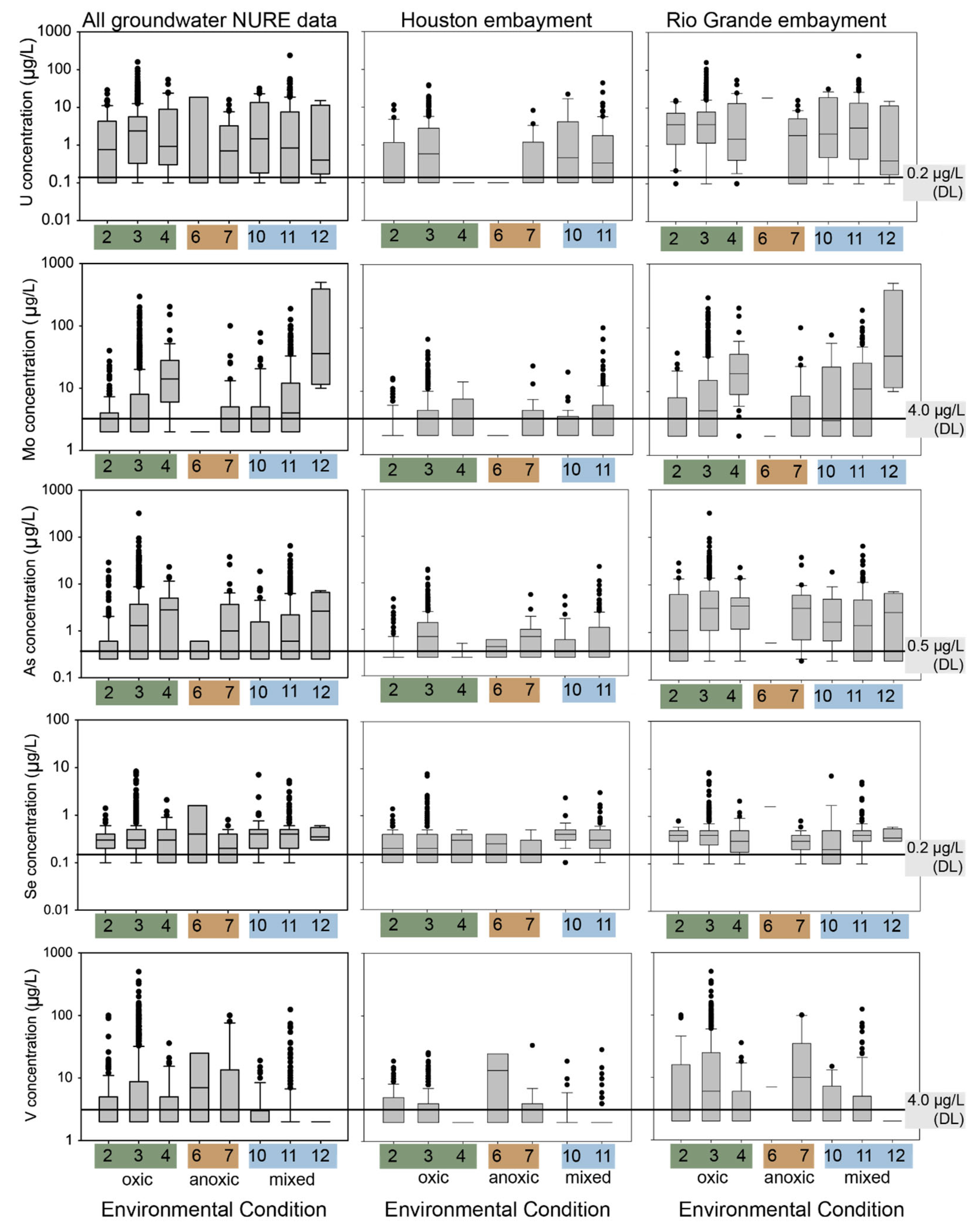
4.1. NURE Groundwater and Surface Water Data

Of the 2302 data points in the NURE groundwater dataset, 1348 had data for the major ions to plot piper diagrams ([70]; Figure S12a). The major ion chemistry of groundwater in the Rio Grande and Houston embayment are similar with the exception of more sulfate (SO42) in the Rio Grande embayment (Figure S12b) than the Houston embayment (Figure S12c). Of the 915 data points in the NURE surface water dataset, 208 had data for the major ions to plot piper diagrams (Figure S12d). The samples in the Houston embayment had more data than the Rio Grande embayment with 185 and 23 useable data points, respectively. However, there were no data for chloride (Cl) in the Rio Grande embayment and only two values in the Houston embayment. The major ion chemistries of surface water in the Rio Grande and Houston embayments (Figure S12e,f) are similar, with the exception of a broader range of Ca in the Houston embayment.
The spatial distribution of COPC concentrations from the NURE groundwater dataset along the South Texas Coastal Plain revealed similar spatial patterns of concentrations of U, As, Mo, and V, with generally higher concentrations in the Rio Grande embayment (Figures S13 and S14 and Tables S5 and S6). The distribution of Se revealed variable concentrations throughout the South Texas Coastal Plain in Permissive Tract 3; however, the Se concentrations are generally less than 1 μg/L.

4.2. Groundwater and Surface Water Distribution by EC

The dominant EC modes within the HUC12 areas were EC3 (pH ≥ 6.5 to <8.5, oxic) for both NURE groundwater and surface water (Figure 4a,b), followed by EC2 (pH ≥ 3 to <6.5, oxic) for groundwater and EC7 (pH ≥ 6.5 to <8.5, anoxic) for surface water. The greatest total number of samples were assigned to the EC3 category for both groundwater and surface water (Figure 4c). For both groundwater and surface water, EC7 (pH ≥ 6.5 to <8.5, anoxic) mainly occurred in the Rio Grande embayment, which is closer to the locations of known U deposits (Figure 1, Figure 4a,b and Figure S8). The surface waters defined as anoxic were located in the Rio Grande embayment and typically had elevated Fe concentrations, which may have affected redox category results. Furthermore, streams in this area have been documented with occasional low dissolved oxygen or anoxic zones [71,72]. The Houston embayment has more occurrences of EC2 (pH ≥ 3 to <6.5, oxic) in groundwater than did the Rio Grande embayment. There are few occurrences of EC2 in surface water in the Houston embayment, but the data are limited.
The majority of COPCs are greater than the DL for the specific element, suggesting that the COPCs are mobile across the pH values and redox assignments in this study (Figure 5, Figures S13 and S14, Tables S1, S5 and S6). The separation of the data by the Houston and Rio Grande embayments shows that the COPCs from the NURE groundwater data have higher concentrations in the Rio Grande embayment than the Houston embayment (Figure 5, Figure S13, Table S5). For instance, the median concentrations of U are higher in all ECs of the Rio Grande embayment except for EC12, and the largest median concentrations of U in the Rio Grande embayment are in EC2, 3, and 11 (Figure 5). This is likely because the Rio Grande embayment has known sources of U and co-occurring elements while the Houston embayment does not [9]. These results suggest that the mobility, occurrence, and persistence of the COPCs is possible throughout the South Texas Coastal Plain where there is a source of the COPCs in the region.

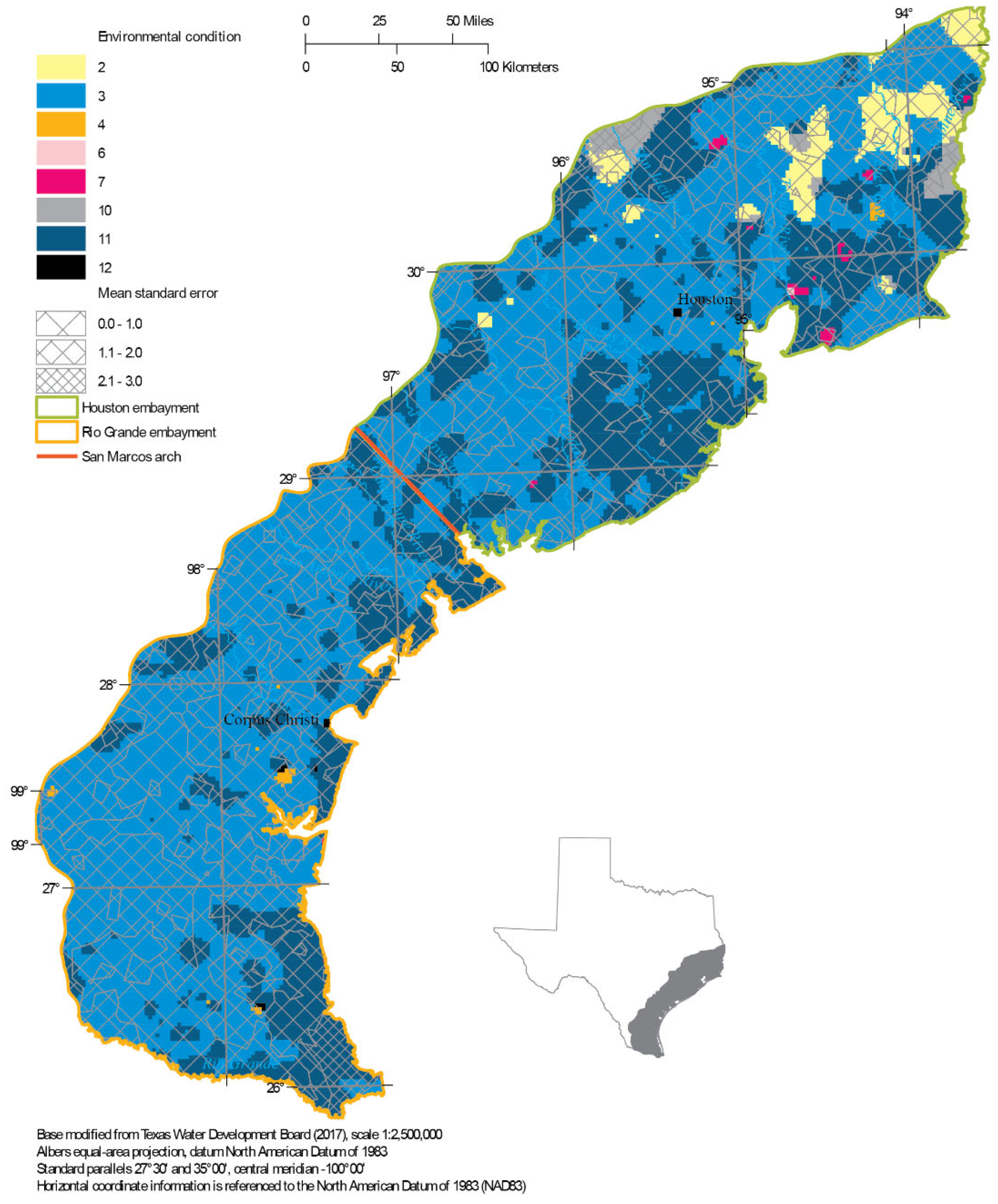
4.3. Variance-Qualified Environmental Condition Maps

Similar to the HUC12 results for the NURE groundwater data, the dominant EC in Permissive Tract 3 resulting from the kriging process described in Section 3.10 was EC3 (pH ≥ 6.5 to <8.5, oxic) (Figure 6), covering about 73 percent of the permissive tract followed by EC2 (pH ≥ 3.0 to <6.5, oxic) and EC11 (pH ≥ 6.5 to <8.5, mixed) covering about 13 and 9 percent of the permissive tract, respectively. The Rio Grande embayment has some areas coded as EC7 (pH ≥ 6.5 to <8.5, anoxic), mainly in the area closer to locations of known U deposits (Figure 1, Figure 4a,b and Figure S8). In the north part of the Houston embayment, more occurrences of EC2 (pH ≥ 3 to <6.5, oxic) in groundwater were estimated than in the Rio Grande embayment.
The confidence found in Permissive Tract 3 is relatively low around the edges, with a large area of low confidence to the northeast of Permissive Tract 3 and near the coast to the south where there were high mean standard errors (Figure 6). These areas of low confidence are directly related to the amount of data available in those areas. In order to increase the confidence in these areas, additional data is needed.
The results from the variance-qualified EC grid of the NURE groundwater data compare well to the results of the HUC12 mode analysis. Both analyses show that EC3 (pH ≥ 6.5 to <8.5, oxic) is the dominant condition in Permissive Tract 3, and when visually compared, the locations of EC2, EC4, EC7, EC10, and EC11 between the two are spatially similar. There are some more detailed changes in the variance qualified EC grid, which is expected because of the finer detail in the interpolation of the data between points and not discretizing the data into HUCs.

4.4. Applying the Geochemical Framework

As a validation, the framework developed in this study was applied to determine how well it predicts the groundwater quality data from the Texas Water Development Board [45] from 1980 to present. The TWDB data were processed and analyzed according to the methods described herein and classified according to the geochemical framework. Results reveal a similar distribution of environmental conditions by HUC compared to the NURE groundwater dataset used to develop the framework (Figure 7 and Figure S15), with the exception of some HUCs plotted from the TWDB dataset that are EC7 and which were EC3 in the NURE data. The distributions of COPC concentrations from the TWDB and NURE data are similar, with the exception of Se, which has a higher overall median in the TWDB data (Figure S15).
The majority of TWDB data HUCs contain the criteria for EC3 (pH ≥ 6.5 to <8.5, oxic), followed by EC7 (pH ≥ 6.5 to <8.5, anoxic) and EC2 (pH ≥ 3 to <6.5, oxic). There are 801 HUCs in the clipped area shown in both maps in Figure 6. The NURE groundwater data cover 520 HUCs and the TWDB groundwater data cover 426 HUCs. EC3 accounts for 76% of the NURE groundwater HUCs and 64% of the TWDB HUCs. The TWDB EC7 covers 27% of the HUCs and many of those areas are plotted as EC3 in the NURE data. The only difference between EC3 and EC7 is the redox condition; oxic to anoxic, respectively. The TWDB may contain more redox-sensitive data that help to better define the redox condition as anoxic or conditions in these HUCs may have changed. In addition, the TWDB data are newer and may contain more accurate data as sampling and analytical protocols are updated. The data from both the NURE and TWDB datasets were grouped across all formations discussed in Section 2.2. Oden and Szabo (2015) note that the majority of water sampled from the stratigraphically lower Evangeline aquifer in the Houston, Texas area have anoxic conditions compared with the Chicot aquifer, which has predominantly oxic conditions. This may also explain the change from EC3 to EC7 in some HUCs of the comparative analysis between the NURE and TWDB data. However, we did not evaluate the number of water samples collected from each formation.

4.5. Applying Kriging to the Texas Water Development Board Data

The majority of TWDB groundwater data in Permissive Tract 3 was EC3 (pH ≥ 6.5 to <8.5, oxic), covering about 63 percent of the permissive tract, and EC11 (pH ≥ 6.5 to <8.5, mixed), covering about 32 percent of the permissive tract (Figure 8). There is a small area of EC2 (pH ≥ 3 to <6.5, oxic) in the north part of the Houston embayment, covering about four percent of the permissive tract. Aside from some small-scale features, the Rio Grande embayment contains mostly EC3 and EC11, while the Houston embayment mostly contains EC2 (pH ≥ 3 to <6.5, oxic), EC3 (pH ≥ 6.5 to <8.5, oxic), and EC11 (pH ≥ 6.5 to <8.5, mixed).
The confidence found in Permissive Tract 3 for the TWDB groundwater data is highly variable throughout the permissive tract (Figure 8). In the Houston embayment, the lower confidence areas, as represented by high mean standard errors, are generally to the north, with an area near the coast east of Houston, Texas. Most of the Rio Grande embayment had mean standard errors above 1.0, showing higher variability in the kriging results, which could be a result of lacking data in the area. In order to increase the confidence in these areas, additional data is needed.
The results from the variance-qualified EC grid of the TWDB groundwater data compare well to the results of the HUC12 mode analysis, except that the HUC12 mode analysis showed more anoxic conditions, as represented by EC7 compared to the mixed conditions of EC11 found in the variance-qualified EC grid. The reason this occurred is as a result of interpolating the DO concentrations of the permissive tract and using the mode for the HUC12 analysis. Overall, the TWDB groundwater data lacked many DO concentrations throughout the dataset; most of the time, the DO concentrations were from samples in the locations represented as EC7 in the HUC12 analysis. Because of the number of samples without DO concentrations, the mode in those HUCs resulted in less oxic conditions (more samples containing no DO concentrations than samples with a DO concentration). The kriging method interpolates all known DO concentrations across the samples that do not have a DO concentration. This interpolation results in those samples with no DO concentration being represented as more oxic, causing the conditions in those locations to change from anoxic to mixed conditions. Besides the difference between EC7 from the HUC12 analysis and EC11 from the variance-qualified EC grid, the other ECs visually compared well between the two analyses.

5. Discussion

The combination of twelve environmental conditions defined in this study and the distribution of COPCs together identified locations where COPCs may occur, persist, or be mobile in groundwater and surface water along the Texas Coastal Plain. When evaluating these results, it is important to remember that there are multiple reasons why these COPCs might be associated with a solid or aqueous phase. The four main conditions that can affect element mobility are (1) environmental conditions such as pe and pH; (2) sorption possibility, with emphasis on solids such as iron oxides and clays; (3) precipitation possibility, with emphasis on reduced sulfur; and (4) the chemical form of the element, which depends on pe, pH, and the presence of other elements. Mobility can be affected by complexation or competition, which relates directly to condition 4.
For discussion of the geochemical framework created in the work presented here, the results from the NURE groundwater data are used. The range of reported COPC concentrations by EC was compared to detection limits to define mobility (Figure 5, Tables S1 and S5 and Figure S11). To document the mobility of each COPC and compare them to the Smith (2007) and Perel’man (1986) models (Table 3), the results were compared to pe-pH diagrams for each COPC (Figure 3), a general understanding of sorption and precipitation of each element especially as in the presence of iron substrate and sulfur species, and results of PHREEQC (57) modeling to identify the chemical form of each element by EC in the Rio Grande embayment (Table S7). Uranium ternary complexes were not included in the PHREEQC modeling for the purposes of this geochemical framework. However, evaluating the ternary complexes for a specific site could further the understanding of U mobility. It is also important to note that the distribution of COPC concentrations varies depending on location along the South Texas Coastal Plain, such as the Houston embayment versus the Rio Grande embayment. The Smith (2007) approach, Perel’man (1986) approach, and the approach described in this text have slightly different geochemical frameworks but similar results. Table 3 provides a summary of each environmental condition and the resulting mobility prediction for each framework. The table includes potential mobility/immobility in association with Fe substrates and H2S.
The oxidation states and species of the COPCs modeled from the NURE groundwater data in PHREEQC indicated the likely form of each COPC. Details of the PHREEQC model are included in the “COPC Oxidation states and species” section of the Supplementary Materials. Results can be compared to Table S1 information and Figure 3 pe-pH diagrams of element species. While the compiled table (Table 3) of mobility predictions does not explicitly include the oxidation states or species of each COPC, the authors took this into consideration when creating the table.
The dominant EC in the Texas Coastal Plain, using the NURE groundwater data, was EC3 (pH ≥ 6.5 to <8.5, oxic). According to the pe-pH diagrams (Figure 3) and the results shown in Figure 6 and S13, this EC would likely promote the mobility of all COPCs. However, if Fe substrates were present, As, Mo, and V could be scarcely mobile in EC3. The next most dominant ECs along the Texas Coastal Plain are EC7 (pH ≥ 6.5 to <8.5, anoxic) and EC2 (pH ≥ 3 to <6.5, oxic). In EC7, As, Mo, Se, and V would be mobile, and U would be immobile. In addition, depending on the specific chemistry of the water and element species, Se and V could be scarcely mobile in EC7. If Fe substrates were present, As would be immobile and the reduced form of Se could be scarcely mobile. If H2S was present, As, Mo, and Se could become immobile as sulfides. In EC2, As, Mo, Se, U, and V would be mobile and As, Mo, U, and V would be immobile if Fe substrates were present. Overall, U, Se, and V could precipitate in the pe-pH ranges of this study, especially under anoxic or mixed conditions (Table 3).
The mobility of COPCs in samples across the mixed redox conditions could be evaluated by pH alone. Given the complexity of the concept of a mixed redox condition, further evaluation could be given to the COPC distribution in ECs 9 to 12.
The Rio Grande embayment had more NURE groundwater samples with COPC concentrations above the DL than the Houston embayment (Figure 4, Figure 5 and Figure 6, Tables S5 and S6, Figure S11). Furthermore, the concentration ranges of COPCs were generally higher in the Rio Grande embayment. This is potentially due to the lack of source rocks with these minerals in the Houston embayment, or that the minerals exist and are not exposed. Importantly, if the Houston embayment had a source of these COPCs or they were introduced to the Permissive Tract 3 aquifers, the elements could occur and persist as they do in the Rio Grande embayment.

5.1. Implications for Planning

This geochemical framework model provides the historical spatial distributions of groundwater and surface water geochemical conditions by redox condition and pH. This information can be used on the South Texas Coastal Plain to identify areas of groundwater and surface water that are favorable to the mobilization of COPCs. For instance, in an area of groundwater or surface water that is categorized as having an EC of 3 (that is, near-neutral pH and oxic), U is likely to be mobile. If that water migrated into an EC with reducing conditions, such as EC7, then you would expect U to precipitate. The median concentration of U from the NURE groundwater data is higher in EC3 than in EC7 (Figure 5), which supports this interpretation. If a sample is located in a HUC categorized as EC12 and migrates to a HUC categorized as EC7, Se and V could become mobile. The data presented in Figure 5 support this example for V, where the median concentration in EC 12 is lower than in EC7. For Se, the median values are slightly higher in EC12 compared to EC7 in the NURE groundwater data. This difference could be related to a geochemical mechanism not addressed in this study.
If possible, facilities that might release the COPCs to the environment could be planned in areas where the COPCs are not mobile. Or, if this is not possible, knowing that the COPCs are mobile could aid in planning water-management strategies on-site.

5.2. Limitation on the Model

The geochemical framework proposed here has limitations, as is the case with any model. This framework is a simplification of a complex system that provides a generalized assessment of the principal factors (pH and redox) that affect the potential for COPCs to be mobile in aquifers and surface waters. The effect of iron substrates and sulfides are difficult to quantify based on water quality data alone and are often heterogeneous throughout aquifer systems. Furthermore, the initial oxidation state and species of the COPCs considered here were not explicitly used to define mobility. The surface water samples may not be in redox equilibrium, which could alter the results of the model (70). The lack of radium data was also a limitation of the study, as radium is often a COPC associated with U mining.
The scale of the HUCs used for the analysis in this study may be larger than what might be needed for U extraction environmental evaluations. A smaller-scale grid could be created and used for this need. The aquifers for this study were combined for data analysis. Separating aquifers by depth could provide a more detailed understanding of the mobility of COPCs. The approach created herein provides a broad view of how to address these questions and can be modified for specific locations and questions. Using this geochemical framework to identify the occurrence of COPCs associated with ore deposits could be evaluated at a smaller scale than HUC12. The user should consider these factors and others in assessing the mobility of COPCs in their study area. However, this framework provides a generalized approach to map locations where elements could occur, persist, or be mobile.

6. Conclusions

This study focused on the South Texas Coastal Plain and the corresponding Gulf Coast aquifer system as a prototype location to create and validate a geochemical framework to understand the mobility of potential COPCs. The geochemical framework developed herein provides a quantitative approach to evaluate the spatial distribution for the occurrence, persistence, and mobility of COPCs based on pH and redox conditions, which were broken into 12 environmental conditions. The effects of iron substrates and H2S on element mobility were also evaluated and discussed qualitatively. The results indicate that the environmental conditions can be used to identify locations where COPCs could occur, persist, or be mobile and how a change in EC could affect the mobility. The methodology has broad applicability to other areas where sufficient water-quality data exist and where the geologic framework is known.

Supplementary Materials

The following are available online at https://www.mdpi.com/article/10.3390/min12040411/s1, Figure S1: A. Generalized map and B. geologic cross section A-A’ and C. generalized map and D. geologic cross section B-B’ in the South Texas Coastal Plain, Figure S2: The major rivers in the Texas Coastal Plain shown in blue and locations of major cities shown in white. An outline of Permissive Tract 3 and the San Marcos arch are shown. Figure S3: Graphs showing pH distribution from NURE groundwater data in each redox category (oxic, mixed, and anoxic), assigned using the Jurgens et al. (2009) redox calculator, by sample number. Figure S4: Pe-pH diagrams of A. Fe (1.79 × 10⁻⁷ mol/L), B. Fe (1.63 × 10⁻⁵ mol/L), C. Mn (3.64 × 10⁻⁸ mol/L), D. Mn (6.94 × 10⁻⁵ mol/L), E. SO42− (2.60 × 10⁻⁵ mol/L), F. SO42− (3.17 × 10⁻² mol/L), G. Fe and SO42− (1.79 × 10⁻⁷ mol/L and 2.60 × 10⁻⁵ mol/L), and H. Fe and SO42− (1.63 × 10⁻⁵ mol/L and 3.17 × 10⁻² mol/L). Element concentrations are the lowest and highest concentration in the NURE groundwater dataset. The pH range of the NURE groundwater dataset (3.0 to 12) is shown on each pe-pH diagram as a red box. Figure S5: Pe-pH diagram showing approximate regions of typical environmental systems (modified from Grundl et al. 2011). The purple box highlights the range of pH values in this study. The blue circles highlight potential water types in the study area. Figure S6. Sequence of microbially mediated redox processes (modified after Stumm and Morgan, 1981). The red ovals highlight potential redox processes occurring in the Texas Coastal Plain based on data available in NURE groundwater samples. The purple box highlights the potential range of pe values in the study area. Figure S7. Saturation indices across pH for pyrite, goethite, hematite, magnetite, maghemite, jarosite, Fe(OH)3(a), and Fe3(OH)8, Fe(OH)2.7Cl0.3 calculated from NURE groundwater data. Graphs are separated by redox condition A. anoxic, pe = −8, B. mixed, pe = 0, and C. oxic, pe = +11. Figure S8. Location of salt domes, mines, and H2S odor detected in NURE groundwater samples along the Texas Gulf Coast. Figure S9. Plot of NURE groundwater SO42− concentrations in mol/L versus pH and calculated equilibrium H2S and HS concentrations in mol/L versus pH. Figure S10. Variograms showing the correlation between the variance of all paired NURE values and the spatial distance between those paired values for the observed (black line in the top window) and modeled (variogram model; red line in the top window) data as well as the number of sampled value pairs compared to distance between paired values (black line in the bottom window) for pH, (B) DO, (C) SO4, (D) Mn, (E) Fe, and (F) S. Figure S11. Variograms showing the correlation between the variance of all Texas Water Development Board paired values and the spatial distance between those paired values for the observed (black line in the top window) and modeled (variogram model; red line in the top window) data as well as the number of sampled value pairs compared to distance between paired values (black line in the bottom window) for (A) pH, (B) DO, (C) SO4, (D) Mn, (E) Fe, and (F) S. Figure S12. A. Spatial distribution of NURE groundwater points with complete datasets to plot piper diagrams. B. Piper diagram of data from the Rio Grande embayment. C. Piper diagram of data from the Houston embayment. D. Spatial distribution of NURE surface water with complete datasets to plot piper diagrams. E. Piper diagram of data from the Rio Grande embayment. F. Piper diagram of data from the Houston embayment. Figure S13. Figures of NURE groundwater COPCs concentrations in micrograms per liter plotted as less than or equal to the detection limit, two times the detection limit, three times the detection limit, four times the detection limit, and samples greater than four times the detection limit. Figure S14. Figures of NURE surface water COPCs concentrations in micrograms per liter plotted as less than or equal to the detection limit, two times the detection limit, three times the detection limit, four times the detection limit, and samples greater than four times the detection limit. Figure S15. TWDB groundwater data by EC compared to NURE groundwater data by EC. Table S1: Geochemical mechanisms associated with constituents of concern, Table S2: Electron acceptors and threshold concentrations used in the redox calculator (Jurgens et al. 2009). Table S3: Henry’s Law values and results of aqueous H2S concentrations, Table S4: Equilibrium aqueous concentrations of sulfur species from pyrite, mackinawite, and gypsum modeled in PHREEQC. Table S5: NURE groundwater constituent of potential concern data compared to the detection limit. The number of samples greater than the detection limit, the percent of the total sample size greater than the detection limit, and the number of samples in each environmental condition (EC) are shown. Table S6: NURE surface water constituent of potential concern data compared to the detection limit. The number of samples greater than the detection limit, the percent of the total sample size greater than the detection limit, and the number of samples in each EC are shown. Table S7: Oxidation state and dominant species for relevant environmental conditions in the Rio Grande embayment. References [73,74,75,76,77,78,79,80,81,82,83,84,85,86] are cited in the Supplementary Materials.

Author Contributions

J.M.B. contributed to: conceptualization, methodology, validation, formal analysis, investigation, data curation, writing—original draft preparation, writing—review and editing, visualization. K.W.-D. and T.J.G. contributed to: supervision, project administration, and funding acquisition. J.M.B., K.W.-D., T.J.G., D.B.Y., D.H., V.S., A.T. and K.B. contributed to conceptualization, methodology, validation, formal analysis, investigation, data curation, visualization. All authors have read and agreed to the published version of the manuscript.

Funding

Authors acknowledge funding support from the Environmental Health Program of the U.S. Geological Survey Ecosystem Mission Area.

Data Availability Statement

The data used in this work can be found at https://mrdata.usgs.gov/nure/water/ and https://www.twdb.texas.gov/groundwater/data/gwdbrpt.asp. (Both accessed on 1 March 2022).

Acknowledgments

The authors thank Kathy Smith and stakeholders in Texas for their input on this work. The work by Delbert Humberson was done while serving as a Hydrologist with the U.S. Geological Survey. This product has been peer-reviewed and approved for publication consistent with U.S. Geological Survey Fundamental Science Practices (https://pubs.usgs.gov/circ/1367/, accessed on 1 March 2022). Any use of trade, firm, or product names is for descriptive purposes only and does not imply endorsement by the U.S. Government. Writings prepared by U.S. Government employees as part of their official duties, including this paper, cannot be copyrighted and are in the public domain.

Conflicts of Interest

The authors declare no conflict of interest.

References

  1. Haines, S.S.; Diffendorfer, J.E.; Balistrieri, L.; Berger, B.; Cook, T.; DeAngelis, D.; Doremus, H.; Gautier, D.L.; Gallegos, T.; Gerritsen, M.; et al. A framework for quantitative assessment of impacts related to energy and mineral resource development. Nat. Resour. Res. 2013, 23, 3–17. [Google Scholar] [CrossRef] [Green Version]
  2. Jenni, K.E.; Pindilli, E.; Bernknopf, R.; Nieman, T.L.; Shapiro, C. Multi-Resource Analysis—Methodology and Synthesis; U.S. Geological Survey: Reston, VA, USA, 2018; Circular 1442. [CrossRef]
  3. U.S. Geological Survey. Integrated Uranium Resource and Environmental Assessment. 2019. Available online: https://www.usgs.gov/centers/cersc/science/integrated-uranium-resource-and-environmental-assessment?qt-science_center_objects=0#qt-science_center_objects (accessed on 25 April 2019).
  4. Gallegos, T.J.; Walton-Day, K.; Seal, R.R., II. Conceptual Framework and Approach for Conducting a Geoenvironmental Assessment of Undiscovered Uranium Resources: U.S. Geological Survey Scientific Investigations Report 2018–5104; U.S. Geological Survey: Reston, VA, USA, 2020. [CrossRef]
  5. Singer, D.A.; Menzie, W.D.; Sutphin, D.M.; Mosier, D.L.; Bliss, J.D. Mineral deposit density—An update, chapter A. In Contributions to Global Mineral Resource Assessment Research; U.S. Geological Survey Professional Paper 1640; Schulz, K.J., Ed.; 2001; pp. A1–A13. Available online: https://pubs.usgs.gov/prof/p1640a/ (accessed on 1 March 2022).
  6. Ulmer-Scholle, D.S. New Mexico Bureau of Geology & Mineral Resources, Uranium—How Is It Mined? 2019. Available online: https://geoinfo.nmt.edu/resources/uranium/mining.html (accessed on 26 April 2019).
  7. Mudd, G.M. Critical review of acid in-situ leach uranium mining: 1—USA and Australia. Environ. Geol. 2001, 41, 390–403. [Google Scholar] [CrossRef]
  8. Saunders, J.A.; Pivetz, B.E.; Voorhies, N.; Wilkin, R.T. Potential aquifer vulnerability in regions down-gradient from uranium in situ recovery (ISR) sites. J. Environ. Manag. 2016, 183, 67–83. [Google Scholar] [CrossRef] [Green Version]
  9. Hall, S.M.; Mihalasky, M.J.; Tureck, K.R.; Hammarstrom, J.M.; Hannon, M.T. Genetic and grade and tonnage models for sandstone-hosted roll-type uranium deposits, Texas Coastal Plain, USA. Ore Geol. Rev. 2017, 80, 716–753. [Google Scholar] [CrossRef]
  10. Henry, C.D.; Galloway, W.E.; Smith, G.E. Considerations in the Extraction of Uranium from a Fresh-Water Aquifer-Miocene Oakville Sandstone, South Texas; Report of Investigations No. 126; The University of Texas at Austin, Bureau of Economic Geology: Austin, TX, USA, 1982. [Google Scholar]
  11. Smith, K.S. Strategies to predict metal mobility in surficial mining environments. In Understanding and Responding to Hazardous Substances at Mine Sites in the Western United States; DeGraff, J.V., Ed.; Geological Society of America: Boulder, CO, USA, 2007; Volume XVII, pp. 25–45. [Google Scholar] [CrossRef] [Green Version]
  12. Eberts, S.M.; Thomas, M.A.; Jagucki, M.L. The Quality of Our Nation’s Waters—Factors Affecting Public-Supply-Well Vulnerability to Contamination—Understanding Observed Water Quality and Anticipating Future Water Quality; U.S. Geological Survey: Reston, VA, USA, 2013; Circular 1385. [CrossRef]
  13. Smith, S.M. National Geochemical Database—Reformatted Data from the National Uranium Resource Evaluation (NURE) Hydrogeochemical and Stream Sediment Reconnaissance (HSSR) Program. U.S. Geol. Surv. Open-File Rep. 2006, 97–492. Available online: https://pubs.usgs.gov/of/1997/ofr-97-0492/nurehist.htm (accessed on 1 March 2022).
  14. Mihalasky, M.J.; Hall, S.M.; Hammarstrom, J.M.; Tureck, K.R.; Hannon, M.T.; Breit, G.N.; Zielinski, R.A.; Elliott, B. Assessment of Undiscovered Sandstone-Hosted Uranium Resources in the Texas Coastal Plain, 2015: U.S. Geological Survey Fact Sheet 2015–3069; U.S. Geological Survey: Denver, CO, USA, 2015. [CrossRef] [Green Version]
  15. Alam, M.S.; Cheng, T. Uranium release from sediment to groundwater: Influence of water chemistry and insights into release mechanisms. J. Contam. Hydrol. 2017, 164, 72–87. [Google Scholar] [CrossRef]
  16. Adidas, E. Groundwater quality and availability in and around Bruni, Webb County, Texas. s.l. Tex. Water Dev. Board LP-209 1991, 1–57. [Google Scholar]
  17. DeSimone, L.A.; McMahon, P.B.; Rosen, M.R. The Quality of Our Nation’s Waters—Water Quality in Principal Aquifers of the United States, 1991–2010; U.S. Geological Survey: Reston, VA, USA, 2014; Circular 1360. [CrossRef]
  18. U.S. Environmental Protection Agency. Abandoned Mine Site Characterization and Cleanup Handbook. U.S. Environmental Protection Agency [USEPA] 2000, EPA 910-B-00-001. Available online: https://www.epa.gov/sites/production/files/2015-09/documents/2000_08_pdfs_amscch.pdf (accessed on 26 October 2020).
  19. Reedy, R.C.; Scanlon, B.R.; Walden, S.; Strassberg, G. Naturally Occurring Groundwater Contamination in Texas; The University of Texas at Austin Bureau of Economic Geology: Austin, TX, USA, 2011; Available online: http://www.twdb.texas.gov/publications/reports/contracted_reports/doc/1004831125.pdf (accessed on 26 April 2019).
  20. Oden, J.H.; Szabo, Z. Arsenic and Radionuclide Occurrence and Relation to Geochemistry in Groundwater of the Gulf Coast Aquifer System in Houston, Texas, 2007–11: U.S. Geological Scientific Investigations Report 2015–5071; U.S. Geological Survey: Austin, TX, USA, 2015. [CrossRef] [Green Version]
  21. Agency for Toxic Substances & Disease Registry [ATSDR], 2015, Toxic Substances Portal. Available online: https://www.atsdr.cdc.gov/toxguides/ (accessed on 28 January 2020).
  22. Besser, J.M.; Leib, K.J. Toxicity of metals in water and sediment to aquatic biota. In Integrated Investigations of Environmental Effects of Historical Mining in the Animas River Watershed, San Juan County, Colorado; Church, S.E., von Guerard, P., Finger, S.E., Eds.; U.S. Department of The Interior: Washington, DC, USA, 2007; Professional Paper 1651; pp. 837–850. [Google Scholar]
  23. U.S. Environmental Agency. Groundwater and Drinking Water—National Primary Drinking Water Regulations. 2019. Available online: https://www.epa.gov/ground-water-and-drinking-water/national-primary-drinking-water-regulations (accessed on 28 January 2020).
  24. U.S. Environmental Agency. National Recommended Water Quality Criteria—Aquatic Life Criteria Table. 2019. Available online: https://www.epa.gov/wqc/national-recommended-water-quality-criteria-aquatic-life-criteria-table (accessed on 28 January 2020).
  25. National Research Council. Ground Water Vulnerability Assessment: Predicting Relative Contamination Potential Under Conditions of Uncertainty; The National Academies Press: Washington, DC, USA, 1993. [Google Scholar] [CrossRef]
  26. Focazio, M.J.; Reilly, T.E.; Rupert, M.G.; Helsel, D.R. Assessing Ground-Water Vulnerability to Contamination: Providing Scientifically Defensible Information for Decision Makers; U.S. Geological Survey: Reston, VA, USA, 2002; Circular 1224. Available online: https://pubs.usgs.gov/circ/2002/circ1224/ (accessed on 26 October 2020).
  27. Plummer, R.; de Loe, R.; Armitage, D. A systematic review of water vulnerability assessment tools. Water Resour. Manag. 2012, 26, 4327–4346. [Google Scholar] [CrossRef] [Green Version]
  28. Smith, K.S.; Huyck, H.L.O. An overview of the abundance, relative mobility, bioavailability, and human toxicity of metals. In Reviews in Economic Geology, Volumes 6A and 6B; Society of Economic Geologists: Littleton, CO, USA, 1999; pp. 29–70. [Google Scholar]
  29. Perel’man, A.I. Geochemical barriers: Theory and practical applications. Appl. Geochem. 1986, 1, 669–680. [Google Scholar] [CrossRef]
  30. Alekseenko, V.; Maximovich, N.G.; Alekseenko, A.V. Geochemical barriers for soil protection in mining areas. In Assessment, Restoration and Reclamation of Mining Influenced Soils; Bech, J., Bini, C., Pashkevich, M.A., Eds.; Academic Press: Cambridge, MA, USA, 2017; pp. 255–274. [Google Scholar] [CrossRef]
  31. Johannesson, K.H.; Tang, J. Conservative behavior of arsenic and other oxyanion-forming trace elements in an oxic groundwater flow system. J. Hydrol. 2009, 378, 13–28. [Google Scholar] [CrossRef]
  32. Blake, J.M.; Avasarala, S.; Artyushkova, K.; Ali, A.S.; Brearley, A.J.; Shuey, C.; Robinson, W.P.; Nez, C.; Bill, S.; Lewis, J.; et al. Elevated concentrations of U and co-occurring metals in abandoned mine wastes in a northeastern Arizona Native American community. Environ. Sci. Technol. 2015, 49, 8506–8514. [Google Scholar] [CrossRef] [PubMed] [Green Version]
  33. Avasarala, S.; Lichtner, P.C.; Ali, A.S.; Gonzalez-Pinzon, R.; Blake, J.M.; Cerrato, J.M. Reactive transport of U and V from abandoned uranium mine wastes. Environ. Sci. Technol. 2017, 51, 12385–12393. [Google Scholar] [CrossRef] [PubMed] [Green Version]
  34. Wilkin, R.T.; Lee, T.R.; Beak, D.G.; Anderson, R.; Burns, B. Groundwater co-contaminant behavior of arsenic and selenium at a lead and zinc smelting facility. Appl. Geochem. 2018, 89, 255–264. [Google Scholar] [CrossRef] [PubMed]
  35. Plant, J.A.; Baldock, J.W.; Smith, B. The role of geochemistry in environmental and epidemiological studies in developing countries: A review. In Environmental Geochemistry and Health; Appleton, J.D., Fuge, R., McCall, G.J.H., Eds.; Geological Society Pub House: Bath, UK, 1996; pp. 7–22. [Google Scholar]
  36. Borch, T.; Kretzschmar, R.; Kappler, A.; Van Cappellen, P.; Ginder-Vogel, M.; Voegelin, A.; Campbell, K. Biogeochemical redox processes and their impact on contaminant dynamics. Environ. Sci. Technol. 2010, 44, 15–23. [Google Scholar] [CrossRef] [PubMed]
  37. Bourg, A.C.M.; Loch, J.P.G. Mobilization of heavy metals as affected by pH and redox conditions. In Biogeodynamics of Pollutants in Soils and Sediments: Risk Assessment of Delayed and Non-Linear Responses; Salomons, W., Stigliani, W.M., Eds.; Springer: Berlin/Heidelberg, Germany, 1995; pp. 87–102. [Google Scholar] [CrossRef]
  38. Langmuir, D. Aqueous Environmental Geochemistry; Prentice-Hall: Hoboken, NJ, USA, 1997. [Google Scholar]
  39. DeVore, C.L.; Rodriguez-Freire, L.; Ali, A.M.; Ducheneaux, C.; Artyushkova, K.; Zhou, Z.; Latta, D.E.; Lueth, V.W.; Gonzales, M.; Lewis, J.; et al. Effect of bicarbonate and phosphate on arsenic release from mining-impacted sediments in the Cheyenne River watershed, South Dakota, USA. Environ. Sci. Process. Impacts 2019, 21, 456–468. [Google Scholar] [CrossRef] [Green Version]
  40. Kim, M.; Nriagu, J.; Haack, S. Carbonate ions and arsenic dissolution by groundwater. Environ. Sci. Technol. 2000, 34, 3094–3100. [Google Scholar] [CrossRef]
  41. Han, M.; Hao, J.; Christodoulatos, C.; Korfiatis, G.P.; Wan, L.; Meng, X. Direct evidence of arsenic (III)-carbonate complexes obtained using electrochemical scanning tunneling microscopy. Anal. Chem. 2007, 79, 3615–3622. [Google Scholar] [CrossRef]
  42. Jenne, E.A. Adsorption of metals by geomedia: Data analysis, modeling, controlling factors, and related issues. In Adsorption of Metals by Geomedia; Jenne, E.A., Ed.; Academic Press: Cambridge, MA, USA, 1998; pp. 1–73. [Google Scholar]
  43. Smith, K.S. Metal sorption on mineral surfaces: An overview with examples relating to mineral deposits. In Reviews in Economic Geology; Plumlee, G.S., Logsdon, M.J., Filipek, L.F., Eds.; Society of Economic Geologists: Littleton, CO, USA, 1999; Volumes 6A–6B, pp. 161–185. [Google Scholar]
  44. Dong, W.M.; Brooks, S.C. Determination of the formation constants of ternary complexes of uranyl and carbonate with alkaline earth metals (Mg2+, Ca2+, Sr2+, and Ba2+) using anion exchange method. Environ. Sci. Technol. 2006, 40, 4689–4695. [Google Scholar] [CrossRef]
  45. Texas Water Development Board. Groundwater Database Reports. 2020. Available online: https://www.twdb.texas.gov/groundwater/data/gwdbrpt.asp (accessed on 3 April 2020).
  46. Jurgens, B.C.; McMahon, P.B.; Chapelle, F.H.; Eberts, S.M. An Excel workbook for identifying redox processes in ground water. U.S. Geol. Surv. Open-File Rep. 2009, 2009, 1004. [Google Scholar]
  47. U.S. Geological Survey. Mineral Resources On-Line Spatial Data. 2017. Available online: https://mrdata.usgs.gov/geology (accessed on 15 September 2017).
  48. Solis, R.F. Upper Tertiary and Quaternary Depositional Systems, Central Coastal Plain, Texas—Regional Geology of the Coastal Aquifer and Potential Liquid-Waste Repositories; The University of Texas at Austin, Bureau of Economic Geology: Austin, TX, USA, 1981; Report of Investigations No. 108. [Google Scholar]
  49. Chowdhury, A.H.; Turco, M.J. Geology of the gulf Coast Aquifer, Texas. In Aquifers of the Gulf Coast of Texas; Mace, R.E., Davidson, S.C., Angle, E.S., Mullican, W.F., III, Eds.; Texas Water Development Board: Austin, TX, USA, 2006; Report 365; pp. 23–50. Available online: https://www.twdb.texas.gov/publications/reports/numbered_reports/doc/R365/R365_Composite.pdf (accessed on 26 September 2020).
  50. Davis, J.A.; Curtis, G.P.; Randall, J.D. Application of Surface Complexation Modeling to Describe Uranium(VI) Adsorption and Retardation at the Uranium Mill Tailings Site at Naturita, Colorado; U.S. Nuclear Regulatory Commission: Rockville, MD, USA, 2003; NUREG/CR-6820.
  51. Zheng, Z.; Tokunaga, T.T.; Wan, J. Influence of calcium carbonate on U(VI) sorption to soils. Environ. Sci. Technol. 2003, 37, 5603–5608. [Google Scholar] [CrossRef] [PubMed]
  52. McMahon, P.B.; Chapelle, F.H. Redox processes and water quality of selected principal aquifer systems. Groundwater 2008, 46, 259–271. [Google Scholar] [CrossRef] [PubMed]
  53. McMahon, P.B.; Chapelle, F.H.; Bradley, P.M. Evolution of redox processes in groundwater. In Aquatic Redox Chemistry; Tratnyek, P., Grundl, T.J., Haderlein, S.B., Eds.; American Chemical Society: Washington, DC, USA, 2011; Volume 1071, pp. 581–597. [Google Scholar] [CrossRef]
  54. Walton-Day, K.; Macaladay, D.L.; Brooks, M.H.; Tate, V.T. Field methods for measurement of ground water redox chemical parameters. Groundw. Monit. Remediat. 1990, 10, 81–89. [Google Scholar] [CrossRef]
  55. Dixit, S.; Hering, J.G. Comparison of Arsenic(V) and Arsenic(III) sorption onto iron oxide minerals: Implications for arsenic mobility. Environ. Sci. Technol. 2003, 37, 4182–4189. [Google Scholar] [CrossRef]
  56. Davis, J.A.; Meece, D.E.; Kohler, M.; Curtis, G.P. Approaches to surface complexation modeling of uranium (VI) adsorption on aquifer sediments. Geochim. Et Cosmochim. Acta 2004, 68, 3621–3641. [Google Scholar] [CrossRef]
  57. Nicot, J.; Scanlon, B.R.; Yang, C.; Gates, J.B. Geological and Geographical Attributes of the South Texas Uranium Province; The University of Texas at Austin, Bureau of Economic Geology: Austin, TX, USA, 2010; Available online: http://www.beg.utexas.edu/files/publications/cr/CR2010-Nicot-1-QAe5657.pdf (accessed on 18 April 2019).
  58. Galloway, W.E. Epigenetic Zonation and Fluid Flow History of Uranium-Bearing Fluvial Aquifer Systems, South Texas Uranium Province; The University of Texas at Austin Bureau of Economic Geology: Austin, TX, USA, 1982; Available online: http://www.beg.utexas.edu/files/publications/cr/CR1981-Galloway-1_QAe6860.pdf (accessed on 18 April 2019).
  59. Stumm, W.; Morgan, J.J. Aquatic Chemistry: Chemical Equilibria and Rates in Natural Waters, 3rd ed.; John Wiley & Sons, Inc.: New York, NY, USA, 1995. [Google Scholar]
  60. Bethke, C.; Farrell, B. GWB Reference Manual; Aqueous Solutions, LLC: Champaign, IL, USA, 2020; Release 14; Available online: https://www.gwb.com/pdf/GWB14/GWBreference.pdf (accessed on 26 September 2020).
  61. Parkhurst, D.L.; Appelo, C.A.J. Description of Input and Examples for PHREEQC Version 3—A Computer Program for Speciation, Batch-Reaction, One-Dimensional Transport, and Inverse Geochemical Calculations; U.S. Geological Survey: Reston, VA, USA, 2013. Available online: https://pubs.usgs.gov/tm/06/a43/ (accessed on 30 June 2021).
  62. Plumlee, G.S. The environmental geology of mineral deposits. In The Environmental Geochemistry of Mineral Deposits, Part A. Processes, Techniques, and Health Issues; Plumlee, G.S., Logsdon, M.J., Eds.; Society of Economic Geologists: Littleton, CO, USA, 1999; Volume 6A, pp. 71–116. [Google Scholar]
  63. Miao, Z.; Brusseau, M.L.; Carroll, K.C.; Carreon-Diazconti, C.; Johnson, B. Sulfate reduction in groundwater: Characterization and applications for remediation. Environ. Geochem. Health 2012, 34, 539–550. [Google Scholar] [CrossRef] [Green Version]
  64. Hem, J.D. Study and Interpretation of the Chemical Characteristics of Natural Water, 2nd ed.; U.S. Geological Survey: Liston, VA, USA, 1970; Water Supply Paper 1473.
  65. ArcGIS 10.4.1; Esri: Redlands, CA, USA, 2015.
  66. U.S. Geological Survey; U.S. Department of Agriculture. Natural Resources Conservation Service. Federal Standards and Procedures for the National Watershed Boundary Dataset (WBD), 4th ed.; U.S. Geological Survey: Liston, VA, USA, 2013; Techniques and Methods 11–A3; p. 63. Available online: http://pubs.usgs.gov/tm/tm11a3/ (accessed on 1 March 2022).
  67. Mochizuki, A.; Murata, T.; Hosoda, K.; Katano, T.; Tanaka, Y.; Mimura, T.; Mitamura, O.; Nakano, S.; Okazaki, Y.; Sugiyama, Y.; et al. Distributions and geochemical behaviours of oxyanion-forming trace elements and uranium in the Hovsgol-Baikal-Yenisei water system of Mongolia and Russia. J. Geochem. Explor. 2018, 188, 123–136. [Google Scholar] [CrossRef]
  68. Seequent, 2021, Geosoft Technical Workshop—Topics in Gridding: Broomfield, Calif., Seequent. Available online: https://files.seequent.com/MySeequent/technical-papers/topicsingriddingworkshop.pdf (accessed on 27 October 2020).
  69. Isaaks, E.H.; Srivastava, R.M. An Introduction to Applied Geostatistics; Oxford University Press: New York, NY, USA, 1989; p. 561. [Google Scholar]
  70. Piper, A.M. A Graphic Procedure in the Geochemical Interpretation of Water-Analyses. Eos Trans. Am. Geophys. Union 1944, 25, 914–928. [Google Scholar] [CrossRef]
  71. Contreras, C. Historical Data Review on Garcitas Creek Tidal. In Performed as Part of the Tidal Stream Use Assessment under TCEQ Contract No. 582-2-48657 (TPWD Contract No. 108287); Resource Protection Division, Texas Parks and Wildlife Department: Austin, TX, USA, 2003. Available online: https://tpwd.texas.gov/landwater/water/conservation/coastal_studies/uaa/media/garcitas.pdf (accessed on 15 September 2020).
  72. Linam, G.W.; Robertson, S.; Sablan, K.; Burke, R.; Larralde, L.; Donovan, S. Fish Assemblage and Water Quality in the San Antonio River, Texas, between Floresville and Goliad; Inland Fisheries Division, Texas Parks and Wildlife Department: Austin, TX, USA, 2014; River Studies Report No. 22. Available online: https://tpwd.texas.gov/publications/pwdpubs/media/pwd_rp_t3200_1804.pdf (accessed on 15 September 2020).
  73. Galloway, W.E. Uranium mineralization in a coastal-plain fluvial aquifer system: Catahoula Formation, Texas. Econ. Geol. 1978, 73, 1655–1676. [Google Scholar]
  74. Reynolds, R.L.; Goldhaber, M.B. Origin of a south Texas roll-type uranium deposit. I. Alteration of iron-titanium oxide minerals. Econ. Geol. 1978, 73, 1677–1689. [Google Scholar] [CrossRef]
  75. Wilkin, R.T.; McNeil, M.S.; Adair, C.J.; Wilson, J.T. Field measurement of dissolved oxygen: A comparison of methods. Groundw. Monit. Remediat. 2001, 21, 124–132. [Google Scholar] [CrossRef]
  76. Price, V.; Jones, P.L. Training Manual for Water and Sediment Geochemical Reconnaissance; Du Pont de Nemours (EI) and Co., Aiken, SC (USA). Savannah River Lab.; SRL Internal Doc. DPST-79-219, GJBX-420(81); U.S. Department of Energy: Grand Junction, CO, USA, 1979; 104p.
  77. Bolivar, S.L. An overview of the National Uranium Resource Evaluation Hydrogeochemical and Stream Sediment Reconnaissance Program, LA-8457-MS; U.S. Department of Energy, Division of Uranium Resources and Enrichment: Washington, DC, USA, 1980.
  78. Grimes, J.G. NURE HSSR Geochemical Sample Archives Transfer Report Part 3 Geochemical Analysis (K/UR—500-Pt3); Oak Ridge Gaseous Diffusion Plant: Ridge Gaseous, TN, USA, 1984. [Google Scholar]
  79. Hem, J.D. Study and Interpretation of Chemical Characteristics of Natural Waters, 3rd ed.; US Geological Survey Water Supply Paper 2254; U.S. Geological Survey: Reston, VA, USA, 1989; 363p. [Google Scholar]
  80. Schwertmann, U.; Fitzpatrick, R.W. Iron minerals in surface environments. Catena Suppl. 1992, 21, 7–30. [Google Scholar]
  81. Kennedy, V.C.; Zellweger, G.W.; Jones, B.F. Filter pore-size effects on the analysis of Al, Fe, Mn, and Ti in Water. Water Resour. Res. 1974, 10, 4. [Google Scholar] [CrossRef]
  82. Grundl, T.J.; Haderlein, S.; Nurmi, J.T.; Tratnyek, P.B. Chapter 1: Introduction to Aquatic Redox Chemistry in Tratneyk et al., Aquatic Redox chemistry. ACS Symposium Series; American Chemical Society: Washington, DC, USA, 2011. [Google Scholar]
  83. Stumm, W.; Morgan, J.J. Aquatic Chemistry, 2nd ed.; Wiley Interscience: Hoboken, NJ, USA, 1981. [Google Scholar]
  84. Eargle, D.H.; Dickinson, K.A.; Davis, B.O. South Texas Uranium Deposits. AAPG Bull. 1975, 59, 766–779. [Google Scholar]
  85. Hamlin, H.S. Salt domes in the Gulf coast Aquifer. In Texas Water Development Board Report 365: Aquifers of the Gulf Coast of Texas; Mace, R.E., Davidson, S.C., Angle, E.S., Mullican, W.F., III, Eds.; Available online: https://www.twdb.texas.gov/publications/reports/numbered_reports/doc/R365/R365_Composite.pdf (accessed on 1 January 2022).
  86. Smonton, S.; Spears, M. Human health effects from exposure to low-level concentrations of hydrogen sulfide. Occup. Health Saf. 2007, 76, 102–104. [Google Scholar]
Figure 1. Location of hydrologic units, geologic units, and uranium occurrences in southeastern Texas after USGS, 2015. Permissive Tract 3 is shown with green and blue outlines for the section in the Houston and Rio Grande embayments, respectively.
Minerals 12 00411 g001
Figure 2. The steps of the approach for the geochemical framework developed in this study.
Minerals 12 00411 g002
Figure 3. pe-pH diagrams of constituents of potential concern. (A) U (4.20 × 10−10× 10−10 mol/L), (B) U (1.00 × 10⁻⁶ mol/L), (C) U and HCO3 (4.20 × 10⁻¹⁰ mol/L and 9.00 × 10⁻⁵), (D) U and HCO3 (1.00 × 10⁻⁶ mol/L and 1.12 × 10⁻² mol/L), (E) As (3.33 × 10⁻⁹ mol/L), (F) As (4.29 × 10⁻⁶ mol/L), (G) Mo (2.08 × 10⁻⁸ mol/L), (H) Mo (5.12 × 10⁻⁶ mol/L), (I) Se (1.27 × 10⁻⁹ mol/L), (J) Se (1.06 × 10⁻⁷ mol/L), (K) V (3.93 × 10⁻⁸ mol/L), (L) V (9.82 × 10⁻⁶ mol/L). Element concentrations are the lowest and highest concentration in the NURE groundwater dataset. The pH range of the NURE groundwater dataset (3.0 to 12) is shown on each pe-pH diagram as a red box. Uranium ternary complexes were not included in the thermodynamic calculations.
Minerals 12 00411 g003
Figure 4. Mode environmental condition by HUC for (A) NURE groundwater data and (B) NURE surface water data. (C) Distribution of data by environmental condition (EC).
Minerals 12 00411 g004
Figure 5. Box and whisker plots of U, Mo, As, Se, and V NURE groundwater chemistry data by environmental condition within Permissive Tract 3, the Houston embayment, and the Rio Grande embayment. The gray box indicates statistical value boundaries. The boundary of the box closest to zero indicates the 25th percentile, the line in the box indicates the median, and the top of the box indicates the 75th percentile. The whiskers show the 10th and 90th percentiles and the black dots indicate outliers. The detection limit for each element is shown as a black line.
Minerals 12 00411 g005
Figure 6. Environmental conditions and mean standard errors for the NURE data using the kriging methods described in Section 3.10.
Minerals 12 00411 g006
Figure 7. NURE groundwater Environmental Condition (EC) HUCs and Texas Water Development Board groundwater EC HUCs, 1980 to present.
Minerals 12 00411 g007
Figure 8. Environmental conditions and mean standard errors for the TWDB data using the kriging methods described in Section 3.10.
Minerals 12 00411 g008
Table 1. Environmental conditions defined.
Environmental ConditionpH RangeReduction–OxidationNumber of
Samples
EC1<3oxic0
EC2≥3 to <6.5oxic11
EC3≥6.5 to <8.5oxic628
EC4≥8.5oxic66
EC5<3anoxic0
EC6≥3 to <6.5anoxic12
EC7≥6.5 to <8.5anoxic173
EC8≥8.5anoxic16
EC9<3mixed0
EC10≥3 to <6.5mixed3
EC11≥6.5 to <8.5mixed6
EC12≥8.5mixed0
Table 2. Detection limits and maximum contaminant levels for constituents of potential concern.
ElementDetection Limit (NURE) (Smith, 2006)Detection Limit (TWDB, 2020)Drinking-Water Maximum Contaminant Level (USEPA, 2019b)Aquatic Life Freshwater Acute Criteria Maximum Concentration (USEPA, 2019a)Aquatic Life Freshwater Chronic Criteria Continuous Concentration (USEPA, 2019a)
All values in μg/L
U0.21.030none identifiednone identified
Mo4.01.0none identified (70 By WHO (Smedley and Kinniburgh 2017))none identifiednone identified
As0.51.010340150
Se0.22.050none identifiednone identified
V4.001.0none identifiednone identifiednone identified
Table 3. Comparison of mobility based on methods by Smith (2007), Perel’man (1986) and this study. (21) (15) (15) (15; 30; 67; 33; 68; 22; 56; 32; 1; 69).
Smith, 2007Perelman, 1986Blake et al., This Study
Environmental ConditionMobileScarcely Mobile to ImmobileEnvironmental ConditionOxidized WaterReduced Water (no H2S)Reduced Water with H2SEnvironmental ConditionMobileScarcely Mobile to ImmobileFe Substrates PresentH2S Present
Adsorption to Fe SubstrateContact with Reduced Water without H2SH2S IntroducedAdsorption to Fe SubstrateContact with Reduced Water without H2SH2S IntroducedAdsorption to Fe Substrate
Oxidizing with pH < 3As, Mo, Se, U, V--pH < 3As immobileU, Mo immobileAs, Mo, U immobileV, As immobileU, Mo immobile--As, V immobile(1) pH < 3, oxicno data but would expect As, Mo, Se, U, V--As immobile--
Oxidizing with pH > 5 to circumneutral, no iron substratesAs, Mo, Se, U, V--pH 3 to 6.5As, Mo, U, V immobileU, Mo immobileMo, U immobileU immobileU, Mo immobileU immobile--(2) pH ≥ 3 to <6.5, oxic As, Mo, Se, U, V--As, Mo, U, V immobile--
Oxidizing with pH > 5 to circumneutral, abundant iron substratesSeAs, Mo, U, VpH 6.5 to 8.5As, Mo, V potentially immobileU, Mo, Se, V immobileMo, U, Se, V immobile--U, Mo immobileMo, U potentially immobile--(3) pH ≥ 6.5 to <8.5, oxicAs, Mo, Se, U, V--As, Mo, V scarcely mobile--
Reducing with pH > 5 to circumneutral, no hydrogen sulfideAs Mo, Se, U, VpH > 8.5As, Mo, V potentially immobileU, Mo, Se, V, As immobileAs, Mo, U, V immobile--U, Mo immobileU potentially immobile--(4) pH ≥ 8.5, oxicAs, Mo, Se, U, V--As immobile Mo, V scarcely mobile--
Reducing with pH > 5 to circumneutral, with hydrogen sulfide--As, Mo, Se, U, V (5) pH < 3, anoxicno data but would expect As, Mo, Vno data but would expect Se, UAs, V immobileAs, Mo, Se can form solids with sulfide
(6) pH ≥ 3 to <6.5, anoxic As, Mo, VSe, UAs, Se immboileAs, Mo, Se can form solids with sulfide
(7) pH ≥ 6.5 to <8.5, anoxicAs, Mo, Se, VSe, U, VAs immobile, Se scarcely mobileAs, Mo, Se can form solids with sulfide
(8) pH ≥ 8.5, anoxicno data but would expect As, Mo, Se, U, V------
(9) pH < 3, mixedno datano dataSe potentially immobileAs, Mo, Se can form solids with sulfide
(10) pH ≥ 3 to <6.5, mixedUAs, Mo, Se, VSe potentially immobileAs, Mo, Se can form solids with sulfide
(11) pH ≥ 6.5 to <8.5, mixedU, AsMo, Se, VMo, Se immobileAs, Mo, Se can form solids with sulfide
(12) pH ≥ 8.5, mixedU, As, MoSe, VMo mobile--
Publisher’s Note: MDPI stays neutral with regard to jurisdictional claims in published maps and institutional affiliations.

