Article

Three-Dimensional Anisotropic Inversions for Time-Domain Airborne Electromagnetic Data

1
College of Geo-Exploration Science and Technology, Jilin University, Changchun 130021, China
2
College of Earth Sciences, Guilin University of Technology, Guilin 541002, China
*
Author to whom correspondence should be addressed.
Minerals 2021, 11(2), 218; https://doi.org/10.3390/min11020218
Submission received: 14 December 2020 / Revised: 4 February 2021 / Accepted: 19 February 2021 / Published: 20 February 2021
(This article belongs to the Special Issue 3D-Modelling of Crustal Structures and Mineral Deposit Systems)

Abstract

:
Rocks and ores in nature usually appear macro-anisotropic, especially in sedimentary areas with strong layering. This anisotropy will lead to false interpretation of electromagnetic (EM) data when inverted under the assumption of an isotropic earth. However, the time-domain (TD) airborne EM (AEM) inversion for an anisotropic model has not attracted much attention. To get reasonable inversion results from TD AEM data, we present in this paper the forward modeling and inversion methods based on a triaxial anisotropic model. We apply three-dimensional (3D) finite-difference on the secondary scattered electric field equation to calculate the frequency-domain (FD) EM responses, then we use the inverse Fourier transform and waveform convolution to obtain TD responses. For the regularized inversion, we calculate directly the sensitivities with respect to three diagonal conductivities and then use the Gauss–Newton (GN) optimization scheme to recover model parameters. To speed up the computation and to reduce the memory requirement, we adopt the moving footprint concept and separate the whole model into a series of small sub-models for the inversion. Finally, we compare our anisotropic inversion scheme with the isotropic one using both synthetic and field data. Numerical experiments show that the anisotropic inversion has inherent advantages over the isotropic ones, we can get more reasonable results for the anisotropic earth structures.

1. Introduction

Time-domain (TD) airborne electromagnetic (AEM) is an effective and efficient geophysical exploration method that is being widely used in mineral exploration, groundwater, environmental, and engineering investigations [1,2]. Due to its dense spatial sampling and multi-time channels, the large-scale three-dimensional (3D) modeling and inversion for TD AEM is formerly impossible due to slow computations and large memory requirement. In the past two decades, one-dimensional (1D) inversion and imaging methods have mainly been used in the interpretation of TD AEM data [3,4,5,6,7,8,9]. However, for complex 3D earth structures, 1D inversion and imaging methods cannot deliver reasonable results.
To get more accurate inversion results, 3D inversion has become a research focus for AEM data interpretation in recent years. Sasaki [10] achieved the 3D inversion of frequency domain (FD) EM data based on the finite-difference method and the Gauss–Newton (GN) optimization. However, this inversion code is only suitable for simple models with small datasets and will fail when dealing with the large-scale AEM datasets or complex models. The moving footprint method proposed by [11,12] is a breakthrough of 3D AEM inversion. Based on the compactness of AEM system, this method splits a large-scale model into a series of small sub-models, so that the computation can be applied with reasonable computational requirements. When the AEM response and sensitivity matrix of sub-models are calculated, they are mapped to a large-scale model for the unified inversion. Due to the reduced spatial scale of the computational model, the efficiency of 3D AEM inversions can be significantly improved. Liu and Yin [13] further used this technique to realize the 3D inversion of multi-pulse TD AEM data. To overcome the difficulties imposed by using multi-source and multi-channel of TD AEM systems, Oldenburg et al. [14] adopted a direct-solver to quickly solve AEM responses that greatly improves the efficiency of 3D inversions. Based on this research of [14], Yang et al. [15] further proposed the local mesh method that effectively reduces the model dimension and accelerates 3D inversion for large-scale models.
Although the 3D inversions of TD AEM data have become increasingly mature, the inversion models are still based on the assumption of isotropic media. Many studies have shown that anisotropy of subsurface media has serious impacts on the EM data [16,17,18,19,20]. Therefore, anisotropy has become an important research focus for many EM methods, such as in marine controlled-source EM (MCSEM) [21,22,23,24], well-logging [25,26,27,28,29], long-offset transient EM (LOTEM) [30], etc. These anisotropic inversion methods have demonstrated that they can provide more reliable results. However, the effect of electrical anisotropy on AEM methods has been less studied, except for [31,32,33] who discussed the effect of anisotropy on AEM responses. Their results show that using an isotropic model to interpret anisotropic data will deliver erroneous results. Further studies show that AEM signal is affected by earth anisotropy in a quite specific way. If the underground structure is 1D, the source field is purely TE-mode and the underground current mainly flows in the horizontal direction that is insensitive to the vertical conductivity, thus only the lateral resistivity will affect the AEM response. The presence of 3D anomalies will induce vertical current around them but it is usually much weaker than the horizontal one, so that only a small amount of information about the underground electrical structure can be observed.
To improve the accuracy of TD AEM data interpretation, we propose in this paper a 3D inversion algorithm for AEM data inversion in TD using a triaxial anisotropic model. We use the 3D finite-difference algorithm based on the secondary scattered electric field approach [13] and the moving footprint technique [12] to simulate large-scale AEM problems. In the inversion process, we use the adjoint forward modeling of [13] and GN optimization to recover the resistivity of the earth. We test our algorithm on synthetic AEM data and field data acquired from Musgraves, South Australia.

2. Basic Theory

2.1. Governing Equations

We first set up a Cartesian coordinate system in which the vertical z-axis is positive downward. A time harmonic dependence eiωt is assumed, where i = 1 , ω = 2πf, the second order of partial differential equation for the scattered electric field in a 3-axial anisotropic earth can be expressed as [34]
× × E s + i ω μ 0 σ E s = i ω μ 0 J p
where μ 0 = 4 π × 1 0 7 H / m is the magnetic permeability of the free space, E s is the scattered electric field, J p is the effective source current densities for the scattered field that is expressed as J p = ( σ σ p ) E p . σ is the model conductivity, while σ p is the background conductivity. For the 3-axial anisotropic case, the σ and σ p are both diagonal conductivity tensors composed of three principal conductivities, i.e.,
σ = [ σ x σ y σ z ] ,   σ p = [ σ x p σ y p σ z p ]
E p is the primary electric field induced by the current in the background structures. The total electric field is E = E s + E p . The magnetic field can be obtained by the Faraday’s law B = ( i ω ) 1 × E . Expansion of the curl operation in Equation (1) yields
2 E x s y 2 + 2 E x s z 2 2 E y s x y 2 E z s x z i ω μ 0 σ x E x s = i ω μ 0 ( σ x σ x p ) E x p
2 E y s x 2 + 2 E y s z 2 2 E x s x y 2 E z s y z i ω μ 0 σ y E y s = i ω μ 0 ( σ y σ y p ) E y p
2 E z s x 2 + 2 E z s y 2 2 E x s x z 2 E y s y z i ω μ 0 σ z E z s = i ω μ 0 ( σ z σ z p ) E z p
Using the finite-difference formulation to replace the derivatives in Equations (3)–(5), we obtain the final equations system for the secondary electrical field, i.e.,
K E s = s
where K is a large sparse matrix and s is the source term. The magnetic field is calculated by B = LE, where L is a spatial interpolation operator. The AEM modeling for a fully anisotropic earth based on the finite-difference formulation of Equation (1) can be found in [33].
In our presented anisotropic inversion, we only focus on 3-axial anisotropic cases, so we use a simplified version of the code developed by [33] to solve the forward problem. After obtaining the FD AEM responses, we adopt inverse Fourier transform to calculate the TD AEM step responses, i.e.,
B s ( t ) = 1 2 π F ( ω ) i ω e i ω t d ω
where F(ω) are the FD responses and Bs(t) is the TD step responses. Then, the TD AEM responses for arbitrary transmitting wave can be calculated via the convolution [35].
d B ( t ) d t = d I ( t ) d t d B s d t = d 2 I ( t ) d t 2 B s
where I(t) is the transmitting current and dB(t)/dt is the magnetic induction.

2.2. Regularized Inversion

The objective functional φ(m, d) for our anisotropic inversion is defined as
φ ( m , d ) = ( d F ( m ) ) T C d 1 ( d F ( m ) ) + λ ( m m 0 ) T C m 1 ( m m 0 )
where m is a 3 × M matrix for model parameters containing three principal conductivities, F is the forward modeling operator. F(m) denotes the synthetic data vector calculated from the model m, while d denotes the AEM field data. C d and C m are the data covariance matrix and model roughness operator, respectively. λ is the regularization parameter used to balance the relative contributions of data misfit φ d and model smoothness φ m .
Assuming that m n is the model parameters at the nth iteration, J is the sensitivity matrix evaluated at m n , and r = d F ( m n ) is the data residual. Then, the GN equation derived from objective functional in Equation (9) can be written as
( J T C d 1 J + λ C m 1 ) Δ m = J T C d 1 r λ C m 1 m n
which can be solved by preconditioned conjugate gradient (PCG) method for the model update Δm. The model parameters are updated by m n + 1 = m n + α Δ m , where α is determined by a linear search [36].

2.3. Calculation of Sensitivity Matrix for 3-Axial Anisotropic Media

Since the footprint of AEM systems is much smaller than the survey area, a small number of meshes is required for numerical modeling. To reduce the computational cost we introduce the footprint concept into our AEM modeling and inversions. In the following, we first divide the entire model into Nm sub-models based on the AEM footprint and calculate the sensitivity matrix for each sub-model. Then, we rearrange these sensitivity matrices into the entire sensitivity matrix. In the Appendix, we will show how to divide the model domain into sub-models. For the nth sub-model, following [21] on their transversely anisotropic inversion, we derivate both side of Equation (6) with respect to parameters m k x , m k y , m k z of the kth cell and get
K E s m k x , y , z = s m k x , y , z K m k x , y , z E s
Considering that B = LE and E p / m k x , y , z = 0 , we obtain the elements for the sensitivity matrix J ^ n T as
j ^ k , n x , y , z = B m k x , y , z = L ( E s + E p ) m k x , y , z = L K 1 ( s m k x , y , z K m k x , y , z E s )
Assuming a Nedge × 3M matrix
G = ( G x G y G z )
where Nedge is the number of edges,
G x , y , z = { s m 1 x , y , z K m 1 x , y , z E s , s m 2 x , y , z K m 2 x , y , z E s , , s m M x , y , z K m M x , y , z E s }
then the sensitivity matrix can be expressed as
J ^ n T = [ j ^ 1 , n x j ^ 2 , n x j ^ M , n x j ^ 1 , n y j ^ 2 , n y j ^ M , n y j ^ 1 , n z j ^ 2 , n z j ^ M , n z ] T = G T K 1 L T
Let v = K 1 L T , and multiply both sides by matrix K, we get the final equation for the adjoint forward modeling, i.e.,
K v = L T
From Equation (16) we can see that no more work needs to be done for calculating the sensitivity matrix than in an isotropic case. The difference between anisotropic and isotropic inversions is the formation of matrix G, which can be done analytically. There are in total Nd columns in v and L T , so we select the same column of v and L T each time to set up an equation, and then solve the equation to obtain the corresponding column of v. After getting the matrix v, we use Equation (15) to calculate J ^ n T , and resemble each J ^ n T for each sub-model to obtain the entire sensitivity matrix in Equation (10). After finishing the calculation in the FD, we use the inverse Fourier transform and the convolution with the transmiting wave to get the sensitivity matrix for specific waveforms in TD. The workflow for TD AEM inversion is given in Figure 1.

3. Numerical Experiments

In the synthetic data inversion, we use the transmitting wave of the VTEM (versatile time-domain electromagnetic) system from Geotech company (Aurora, ON, Canada) (c.f. Figure 2). The transmitter and receiver assumes a concentric geometry. The height of the transmitting coil is 30 m and the receiver is 0.5 m above the transmitter. To establish the first model for testing, we assume a tilted ore-body buried in a half-space with a distinct strike as shown in Figure 3a. The ore-body is 60 m wide in the x-direction, 360 m long in the y-direction, the top surface is located at z = 10 m, and the bottom surface is located at z = 208 m. The entire model is discretized into 48 × 48 × 13 cells (refer to Appendix for specific grid design). Figure 3b is the distribution of the measuring points. The distance between measuring points is 40 m. For easy understanding, we use the resistivity instead of the conductivity in our following discussions. For synthetic and field survey data, the initial and reference model are both selected as isotropic half-space of 100 ohm-m to implement our anisotropic and isotropic inversions (for the anisotropic cases, we assume the same initial resistivities along three principal axes). The data misfit is calculated by the root mean square (RMS), i.e.,
χ = 1 N i = 1 N ( d i , o b s d i , c a l c ) 2 ε i , o b s 2
where di, obs and di,calc are respectively the observed and predicted data, εi, obs is the estimate of data error, N is the number of data. We use 3% of the syntetic data as the data error estimate in our isotropic and anisotropic inversions. In the iterative inversion process, the initial regularization parameter is set to be 1000. When the RMS difference between the last two iterations becomes less than 0.02, the regularization parameter is reduced to 1/10 of the previous one. When the RMS falls below 1 and the RMS difference between the last two iterations becomes less than 0.002, or the iterations reach the maximum number, the inversion is terminated.

3.1. Synthetic Data Inversion for an Anisotropic Ore-Body

For the first synthetic example, we assume an isotropic background of 100 ohm-m and an anisotropic ore-body (c.f. Figure 3a) with the resistivity tensor of
ρ = ( 30 0 0 0 10 0 0 0 20 ) ohm m
Figure 4 shows the inversion results in slices in the xz-section for three principal resistivities. It is seen that the resistivities in the x- and y-directions are well recovered, but the resistivity in the z-direction is not recovered. This can be easily explained by the characteristic EM wave induced by a TD AEM system. If the earth is 1D, the source field is purely TE-mode and the underground current mainly flows in the horizontal direction, thus the EM field is only sensitive to the resistivity in the x- and y-directions, while it is insensitive to the resistivity in the z-direction for the vertical resistivity ρz has little effect on AEM responses. This explains that although the model is 3D, the current densities in the x- and y-direction are much larger than that in the z-direction. This results in the insensitive EM responses and poor resolvability to the resistivity in the z-direction.
Figure 4d presents the isotropic inversions for the same dataset. Since the synthetic data in this example is calculated from an anisotropic model, it is difficult to fit the data by an isotropic model. Thus, artifacts are introduced into the inversion results. This means that when the data are collected in an area with anisotropy, an anisotropic inversion is necessary. To better locate the ore-body and eliminate the false resistivity distribution in surrounding rocks, we calculate an equivalent resistivity in the horizontal direction using the inversion results of ρx and ρy via the following formula [37]
ρ h = ρ x ρ y
From Figure 4h, we can see that the equivalent resistivity effectively suppresses the fake anomalies brought by the “over anisotropy” phenomenon.
Figure 5 shows the data fitting and RMS curves for the anisotropic and isotropic inversions at profile y = 50 m (the red line in Figure 3b). The data fittings for isotropic and anisotropic inversions are both very well, the RMSs are at the same level. Thus, for anisotropic data, using isotropic model can also achieve a good data fitting, but the underground model is not in line with the actual situation. Thus, it is necessary to implement anisotropic inversion when the earth is anisotropic. From Figure 6a, we can see that both isotropic and anisotropic inversions achieve the same level of RMS with stable convergence. The regularization parameter decreases from the initial 1000 to 0.00001 (Figure 6b).

3.2. Synthetic Data Inversion for Anisotropic Host Rock

In the second synthetic data inversion, we assume that the first layer has a thickness of 100 m and a resistivity of
ρ p = ( 80 0 0 0 40 0 0 0 60 ) ohm m
the second layer is an isotropic half-space with a resistivity of 100 ohm-m. The isotropic anomalous body has a resistivity of 10 ohm-m. Figure 7 shows the inversion results obtained from the synthetic VTEM data. It is seen from the figures that the anisotropic inversion well recovers the structure and resistivity values of the anomalous body in the x- and y-directions. However, like the previous example, the resistivity in the z-direction is not recovered accurately. From Figure 7, we can also see that the anisotropic character of the first layer is not well recovered. The main reason is that we assume a concentric TD AEM system for our synthetic data inversion. If the ore-body is absent, the model can be viewed as a horizontally uniform anisotropic medium and the same response can still be obtained by swapping the resistivity in the x- and y-directions. The presence of a 3D ore-body results in the generation of a vertical current, but the resolution of resistivity in the x- and y-directions in the inversion does not increase much (see Figure 7e–f). From the inversion results in x- and y-direction in Figure 7, we find that in the first layer, the x-direction resistivity has a fake conductive anomaly on the left side, while the y-direction resistivity at the same location is resistive, which means that we find a “over anisotropy” phenomenon in the inversion. Figure 8 shows the horizontal slices of the anisotropic inversion results of ρx and ρy and the equivalent resistivity.
From Figure 7h and Figure 8c, we can see that the equivalent resistivity effectively suppresses the fake anomalies brought by the “over anisotropy”. Although the definition of equivalent resistivity has little exact physical meaning, we can get from its distribution a more reliable model structure. Similarly, from the isotropic inversion results given in Figure 7d, we can draw the same conclusions as in the previous example. The resistivity distribution in the isotropic inversion is relatively messy, and the resistivity varies seriously. The reason for these is that to fit the data, many false anomalies are created to fit the anisotropic structure.
From Figure 9, we can see that both isotropic and anisotropic inversions have good data fitting. From the RMS curves given in Figure 10a, we can see that both isotropic and anisotropic inversions achieve stable convergence. From Figure 10b, the regularization parameter for the isotropic inversion decreases from the initial value of 1000 to 0.00001, while the regularization parameter for the anisotropic inversion decreases from 1000 to 1.

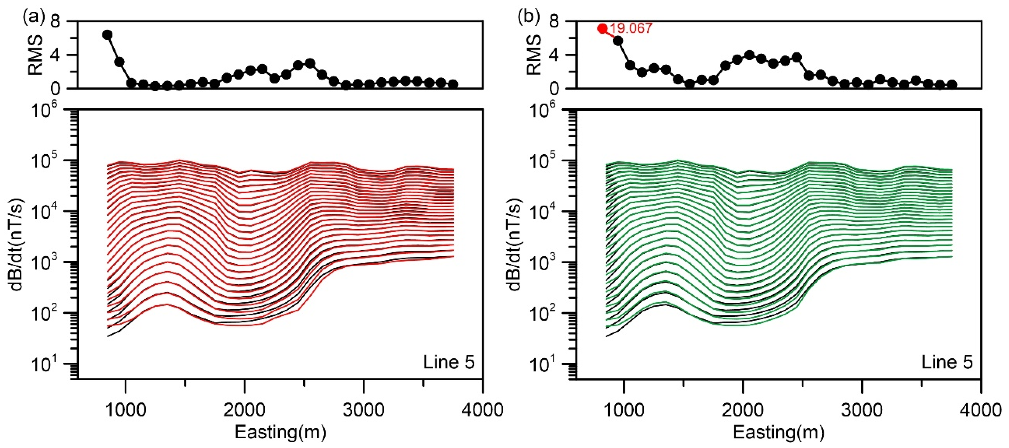
4. Field Data Example

To further demonstrate the effectiveness of our anisotropic inversions, we invert a survey dataset acquired by the VTEM system in Musgrave province, South Australia (Figure 11). This dataset was acquired for mineral prospecting and regional hydro-geological assessment. We select this dataset because this area presents abrupt lateral variations, product of an outcropping mafic intrusive and more subtle lateral continuous sedimentary sequences [38]. The subsurface structure in this area have obvious anisotropy.
For our inversion, we select 210 surveying points along 7 flight lines, marked as white lines in Figure 11. The inverse model is discretized into 178 × 48 × 19 cells. In the central area, the grid sizes in the x- and y-directions are 20 m and 40 m, respectively, while the dimensions of the 4 external grid sizes increase by a factor of 2, symmetrically to both sides of the x- and y-directions. In the z-direction, the thickness of first layer is 10 m, and the thickness of the underlying layers increase by a factor of 1.2 until the 13th layer, the 14th–19th layers are extended layers with thicknesses of 100, 100, 100, 200, 300, and 400 m, respectively. We add 8 external grids in the air layer. The moving footprint is used to divide the entire model into sub-models. The division of sub-model is the same as that of synthetic examples. In the inversion process, we reduce the regularization parameter to 1/10 of the previous value in each iteration and keep it unchanged when it reaches the threshold of 0.001, which can ensure the stable convergence in the inversion. The inversion is terminated when the RMS difference between the last two iterations is less than a threshold of 0.03. We use 3% of the field data as the data error estimate in our isotropic and anisotropic inversions.
Figure 12 presents the comparison of 3D anisotropic and isotropic inversion results. It can be seen from the figures that the resistivity distributions of the anisotropic and isotropic inversions are similar. They show a layered structure, which is consistent with the sedimentary lithology in this area. However, a detailed analysis shows that there exist significant differences in details. First, the anisotropic inversions show a smoother and more continuous layered structure than the isotropic ones. In opposite, the isotropic inversions deliver random results among these lines. The continuity is poor and there is a thick low-resistivity layer in the central region of Line 5, which is quite different from the surrounding lines. Second, in the near surface between x = 1500−2500 m, the anisotropic inversion shows a clear high-resistivity layer in the y-direction, but from the isotropic inversion we cannot see this layer clearly. By comparing Figure 12a,b, we can further see that there exists a big difference between the resistivities ρx and ρy from x = 1000 to 2500 m. However, this cannot be seen from the isotropic inversion results. The artifacts appearing in the anisotropic and isotropic inversions at the beginning of the profile may result from the poor data fitting.
We take as example the horizontal slices of isotropic and anisotropic inversions at the depth of 44m and show them in Figure 13. It is seen that the inverted anisotropic models of ρx in Figure 13a and ρy in 13b are quite different from each other between x = 1500 and x = 2500m, showing the anisotropic characteristics in this area. The equivalent resistivity in Figure 13d is similar to the isotropic inversion results in Figure 13c. This is due to the horizontal current in the earth excited by an AEM system in TD, the EM signal is mainly created by the averaged resistivities in the x- and y-directions, the equivalent resistivity takes most effect, so we can see a coincidence between Figure 13c,d.
To check the data fitting of anisotropic and isotropic inversions, we take Line 5 as an example. Figure 14 shows that these two inversions have the same level of data fitting and overall RMS. However, the data fitting around 1000 m is not good, which is coincidence with the strong resistivity contrast in the inversion results (c.f. Figure 12 and Figure 13). Figure 15 shows the RMSs and regularization parameters for the isotropic and anisotropic inversions. Both inversions have stable convergence and good data fitting. The anisotropic inversion converges faster than the isotropic one. From Figure 15b, the regularization parameter of each iteration decreases by 1/10 and remains unchanged when it reaches 0.001.

5. Conclusions

In this paper, we have successfully applied the anisotropic model to TD AEM data inversion. The numerical examples for both synthetic and field data proved its effectiveness. From the inversions to the synthetic models we find that it is difficult to invert the resistivity in the vertical z-direction from TD AEM data because for an AEM system the induced current in z-direction is much smaller than those in the horizontal x- and y-directions. Another finding from our synthetic examples is that the inversions based on an ansiotropic model may create “over anisotropy”, which, however, can be supressed by the equivalent resistivity calculated from the anisotropic inversion results. Thus, by combining all those inversion results together, we can obtain a reasonable resistivity distribution inside the earth. Further numerical experiment with field survey data demonstrated that compared to the isotropic inversion, the inversion based on an anisotropic model can provide more genuine results than the isotropic one for the TD AEM data collected in an anisotropic area.

Author Contributions

Conceptualization, Y.S. and C.Y.; formal analysis, C.Y. and Y.L.; funding acquisition, C.Y.; investigation, X.R.; methodology, Y.S. and Y.L.; project administration, C.Y.; resources, X.R. and Y.L.; software, Y.L. and Y.S.; supervision, B.Z. and X.R.; validation, B.Z. and B.X.; visualization, Y.L. and Y.S.; writing—original draft, Y.S. and Y.L. All authors have read and agreed to the published version of the manuscript.

Funding

The paper is financially supported by the National Natural Science Foundation of China (42030806, 41774125, 41901104), the Strategic Priority Research Program of the Chinese Academy of Sciences (XDA14020102), Key National Research Project of China: 2018YFC0603300, and the S&T Program of Beijing (Z181100005718001).

Data Availability Statement

Data was obtained from Alan Yusen Ley-Cooper and are available with the permission of Alan Yusen Ley-Cooper.

Acknowledgments

Thanks to Alan Yusen Ley-Cooper for providing the field data. We want to thank three reviewers and editors for their constructive comments and suggestions that improve the clarity of this paper.

Conflicts of Interest

The authors declare no conflict of interest.

Appendix A

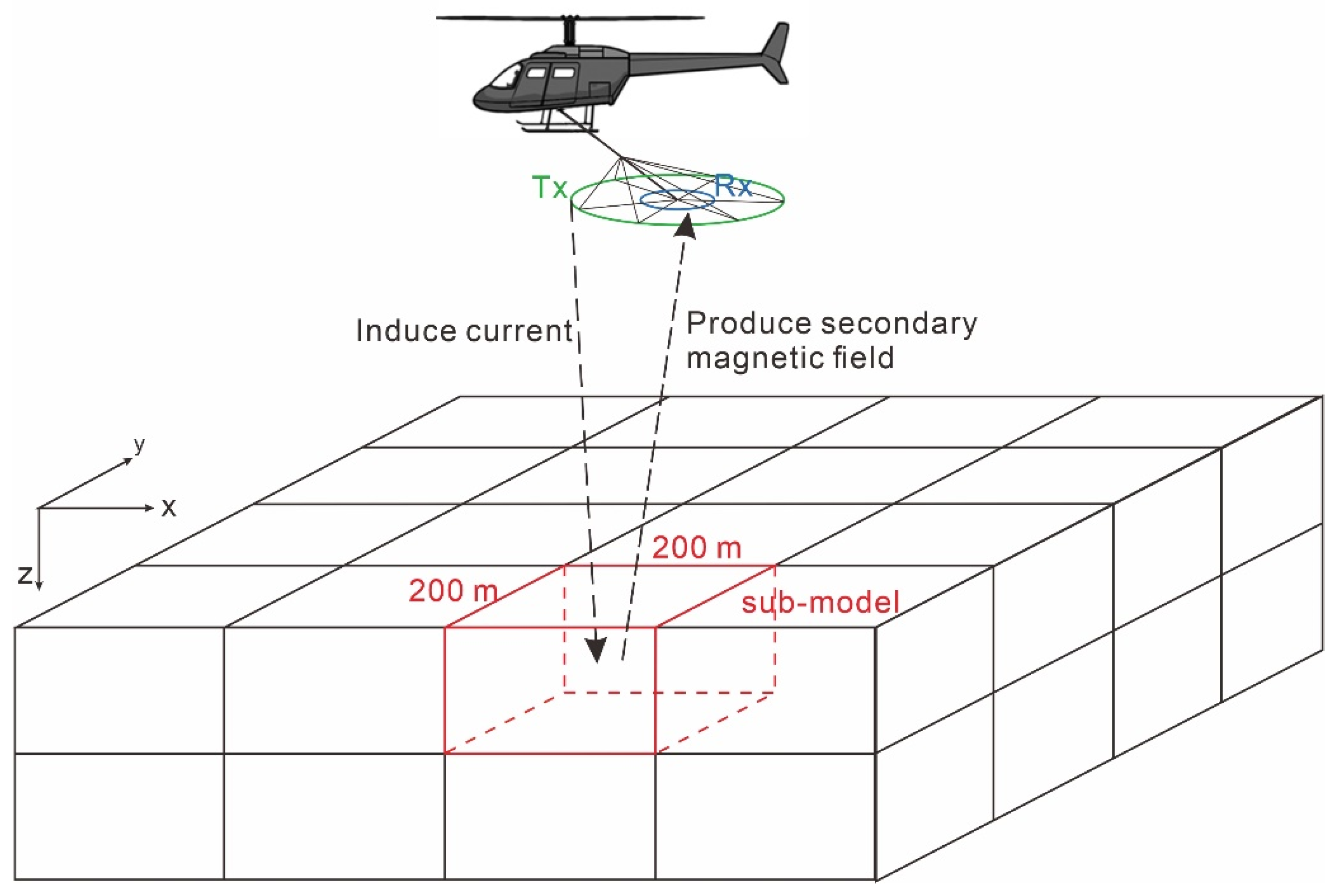
Appendix A.1. Sub-Model Based on the Moving Footprint

For our forward modeling and calculation of the sensitivity matrix based on the “moving footprint”, we extract an area (200 m × 200 m) under each survey site to construct the central area of the sub-model (Figure A1), and then add 4 external grids in the x- and y-directions with the sizes of 40, 80, 160, and 320 m, symmetrically to both sides. We use the volume-averaging technique to calculate the resistivity in the external region. The sub-model area for calculating the sensitivity at each survey site is as large as the footprint, so that there are only few non-zero elements in a row of the overall matrix. The global sensitivity matrix is formed by putting all the sensitivity matrices together. Different from the conventional sensitivity matrix, the sensitivity matrix calculated based on the footprint is sparse and easy to store. The reduction of the model scale greatly improves the model efficiency.
Figure A1. Sub-model based on the moving footprint.
Minerals 11 00218 g0a1

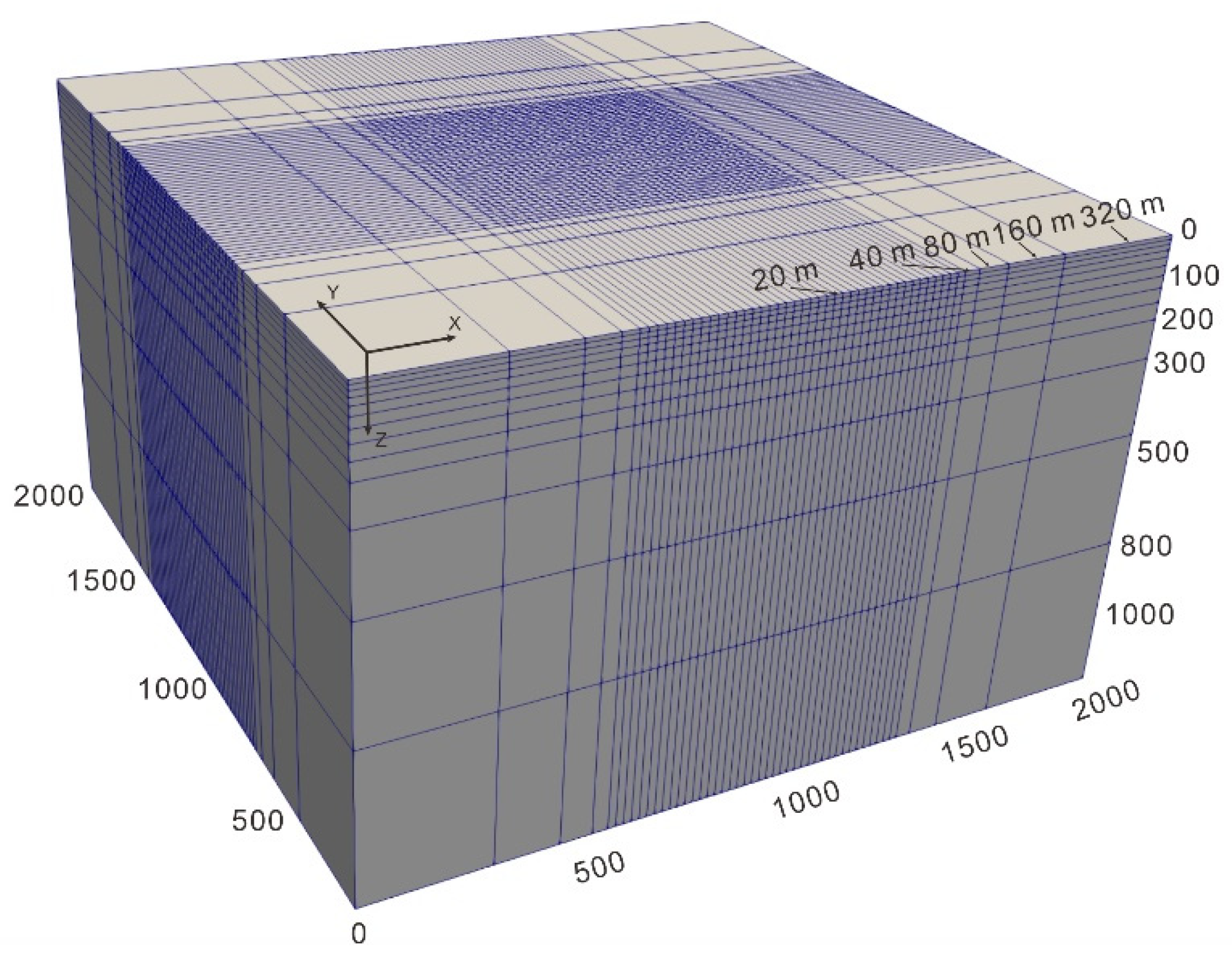
Appendix A.2. Grid Design for Our Synthetic Models

For synthetic modelings, we design the grids as follows. The entire model is discretized into 48 × 48 × 13 cells. The grid sizes in the central area in the x- and y-directions are assumed to be 20 m, and the dimensions of the 4 external grids in the x- and y-directions are 40, 80, 160, and 320 m, symmetrically to both sides. The total extensions in the x- and y-direction are 2000 m. In the z-direction, the thickness of the first layer is 10 m, and the thickness of the underlying layers increases sequentially by a factor of 1.2 until the 9th layer, the 10th–13th layers are extended layers with thicknesses of 100, 200, 300, and 400 m, respectively. The total extension in the z-direction is 1208 m. We add 8 external grids in the air layer. The first two grids in the air have a size of 10 m, and the rest are increased by a factor of 3. The total extension of the air layer in the z-direction is 32,800 m. The final model grids are shown in Figure A2.
Figure A2. Model grids for synthetic examples. (The air layer is not included).
Minerals 11 00218 g0a2

References

  1. Siemon, B.; Christiansen, A.V.; Auken, E. A review of helicopter-borne electromagnetic methods for groundwater exploration. Near Surf. Geophys. 2009, 7, 629–646. [Google Scholar] [CrossRef] [Green Version]
  2. Kaminski, V.; Legault, J.M.; Kumar, H. The Drybones Kimberlite: A case study of VTEM and ZTEM airborne EM results. Aseg Ext. Abstr. 2010, 2010, 1–4. [Google Scholar] [CrossRef] [Green Version]
  3. Chen, J.; Raiche, A. Inverting AEM data using a damped eigenparameter method. Explor. Geophys. 1998, 29, 128–132. [Google Scholar] [CrossRef]
  4. Huang, H.; Fraser, D.C. Dielectric permittivity and resistivity mapping using high frequency, helicopter-borne EM data. Geophysics 2002, 67, 727–738. [Google Scholar] [CrossRef] [Green Version]
  5. Auken, E.; Chistiansen, A.V.; Jacobsen, B.H.; Foged, N.; Sørensen, K.I. Piece-wise 1D laterally constrained inversion of resistivity data. Geophys. Prospect. 2005, 53, 497–506. [Google Scholar] [CrossRef]
  6. Sattel, D. Inverting airborne electromagnetic (AEM) data using Zohdy’s method. Geophysics 2005, 70, G77–G85. [Google Scholar] [CrossRef]
  7. Brodie, R.; Sambridge, M. A holistic approach to inversion of frequency-domain airborne EM data. Geophysics 2006, 71, G301–G312. [Google Scholar] [CrossRef]
  8. Viezzoli, A.; Auken, E.; Munday, T. Spatially constrained inversion for quasi 3D modeling of airborne electromagnetic data—An application for environmental assessment in the Lower Murray Region of South Australia. Explor. Geophys. 2009, 40, 173–183. [Google Scholar] [CrossRef] [Green Version]
  9. Christensen, N.B.; Fitzpatrick, A.; Munday, T. Fast approximate inversion of frequency-domain electromagnetic data. Near Surf. Geophys. 2010, 8, 1–15. [Google Scholar] [CrossRef]
  10. Sasaki, Y. Full 3-D inversion of electromagnetic data on PC. J. Appl. Geophys. 2001, 46, 45–54. [Google Scholar] [CrossRef]
  11. Cox, L.H.; Zhdanov, M.S. Advanced computational methods for rapid and rigorous 3D inversion of airborne electromagnetic data. Commun. Comput. Phys. 2008, 3, 160–179. [Google Scholar]
  12. Cox, L.H.; Wilson, G.A.; Zhdanov, M.S. 3D inversion of airborne electromagnetic data using a moving footprint. Explor. Geophys. 2010, 41, 250–259. [Google Scholar] [CrossRef]
  13. Liu, Y.; Yin, C. 3D inversion for multipulse airborne transient electromagnetic data. Geophysics 2016, 81, E401–E408. [Google Scholar] [CrossRef]
  14. Oldenburg, D.W.; Haber, E.; Shekhtman, R. Three dimensional inversion of multi-source time domain electromagnetic data. Geophysics 2013, 78, E47–E57. [Google Scholar] [CrossRef] [Green Version]
  15. Yang, D.; Oldenburg, D.W.; Haber, E. 3-D inversion of airborne electromagnetic data parallelized and accelerated by local mesh and adaptive soundings. Geophys. J. Int. 2014, 196, 1492–1507. [Google Scholar] [CrossRef] [Green Version]
  16. Régis, C.; da Cruz Luz, E.; Costa, M.D. Inversion of anisotropic MT data using approximate equality constrains. In Proceedings of the 2010 SEG Annual Meeting, Denver, CO, USA, 17–22 October 2010. [Google Scholar]
  17. Häuserer, M.; Junge, A. Electrical mantle anisotropy and crustal conductor: A 3-D conductivity model of the Rwenzori Region in western Uganda. Geophys. J. Int. 2011, 185, 1235–1242. [Google Scholar] [CrossRef] [Green Version]
  18. Miensopusτ, M.P.; Jones, A.G. Artefacts of isotropic inversion applied to magnetotelluric data from an anisotropic Earth. Geophys. J. Int. 2011, 187, 677–689. [Google Scholar] [CrossRef]
  19. Jones, A.G. Distortion decomposition of the magnetotelluric impedance tensors from a one-dimensional anisotropic Earth. Geophys. J. Int. 2012, 189, 268–284. [Google Scholar] [CrossRef]
  20. Guo, Z.Q.; Wei, W.B.; Ye, G.F.; Jin, S.; Jing, J.E. Canonical decomposition of magnetotelluric responses: Experiment on 1D anisotropic structures. J. Appl. Geophys. 2015, 119, 79–88. [Google Scholar] [CrossRef]
  21. Newman, G.A.; Commer, M.; Carazzone, J.J. Imaging CSEM data in the presence of electrical anisotropy. Geophysics 2010, 75, F51–F61. [Google Scholar] [CrossRef]
  22. Tseng, H.-W.; Stalnaker, J.; MacGregor, L.M.; Ackermann, R.V. Multi-dimensional analyses of the SEAM controlled source electromagnetic data—The story of a blind test of interpretation workflows. Geophys. Prospect. 2015, 63, 1383–1402. [Google Scholar] [CrossRef]
  23. Wiik, T.; Nordskag, J.I.; Dischler, E.Ø.; Nguyen, A.K. Inversion of inline and broadside marine controlled-source electromagnetic data with constraints derived from seismic data. Geophys. Prospect. 2015, 63, 1371–1382. [Google Scholar] [CrossRef]
  24. Hoversten, G.M.; Myer, D.; Key, K.; Alumbaugh, D.; Hermann, O.; Hobbet, R. Field test of sub-basalt hydrocarbon exploration with marine controlled source electromagnetic and magnetotelluric data. Geophys. Prospect. 2015, 63, 1284–1310. [Google Scholar] [CrossRef]
  25. Shen, J.S. Modeling of 3-D electromagnetic responses to the anisotropic medium by the edge finite element method. Well Logging Technol. 2004, 28, 11–15. [Google Scholar]
  26. Wang, H.; Tao, H.; Yao, J.; Chen, G. Fast multiparameter reconstruction of multicomponent induction well-logging datum in a deviated well in a horizontally stratified anisotropic formation. IEEE Trans. Geosci. Remote Sens. 2008, 46, 1525–1534. [Google Scholar] [CrossRef]
  27. Yang, S.W.; Wang, H.N.; Chen, G.B.; Yao, D.H. The 3-D finite difference time domain (FDTD) algorithm of response of multicomponent electromagnetic well logging tool in a deviated and layered anisotropic formation. Chin. J. Geophys. 2009, 52, 833–841. (In Chinese) [Google Scholar] [CrossRef]
  28. Beer, R.; Zhang, P.; Alumbaugh, D.; Nalonnil, A. Anisotropy modeling and inversions of DeepLook-EM data from Brazil. In Proceedings of the 2010 SEG Annual Meeting, Denver, CO, USA, 17–22 October 2010. [Google Scholar]
  29. Zhang, G.Y.; Xiao, J.Q.; Hong, D.C.; Yang, S.D. A fast inversion method of 3D induction logging responses in layered anisotropic formation. Well Logging Technol. 2013, 37, 487–491. [Google Scholar]
  30. Liu, Y.; Yogeshwar, P.; Hu, X.; Peng, R.; Tezkan, B.; Morbe, W.; Li, J. Effects of electrical anisotropy on long-offset transient electromagnetic data. Geophys. J. Int. 2020, 222, 1074–1089. [Google Scholar] [CrossRef]
  31. Yin, C.; Fraser, D.C. The effect of the electrical anisotropy on the response of helicopter-borne frequency-domain electromagnetic systems. Geophys. Prospect. 2004, 52, 399–416. [Google Scholar] [CrossRef]
  32. Avdeev, D.B.; Newman, G.A.; Kuvshinov, A.V.; Pankratov, O.V. 3D frequency-domain modeling of airborne electromagnetic responses. Explor. Geophys. 1998, 29, 11–119. [Google Scholar]
  33. Liu, Y.; Yin, C. 3D anisotropic modeling for airborne EM systems using finite-difference method. J. Appl. Geophys. 2014, 109, 186–194. [Google Scholar] [CrossRef]
  34. Newman, G.A.; Alumbaugh, D.L. 3D induction logging problems. Part I. An integral equation solution and model comparisons. Geophysics 2002, 67, 484–491. [Google Scholar] [CrossRef]
  35. Yin, C.; Huang, W.; Ben, F. The full-time electromagnetic modeling for time-domain airborne electromagnetic systems. Chin. J. Geophys. 2013, 56, 3153–3162. (In Chinese) [Google Scholar]
  36. Haber, E. Computational Methods in Geophysical Electromagnetics; SIAM: Philadelphia, PA, USA, 2014. [Google Scholar]
  37. Yin, C. Geoelectrical inversion for a one-dimensional anisotropic model and inherent non-uniqueness. Geophys. J. Int. 2000, 1, 11–23. [Google Scholar] [CrossRef] [Green Version]
  38. Ley-Cooper, A.Y.; Viezzoli, A.; Guillemoteau, J.; Vignoli, G.; Macnae, J.; Cox, L.; Munday, T. Airborne electromagnetic modelling options and their consequences in target definition. Explor. Geophys. 2014, 46, 74–84. [Google Scholar] [CrossRef]
Figure 1. Workflow for time-domain (TD) airborne electromagnetic (AEM) inversion based on the “moving footprint”.
Minerals 11 00218 g001
Figure 2. Transmitting waveform for VTEM system.
Minerals 11 00218 g002
Figure 3. (a) A synthetic model; (b) distribution of measuring points (the red line is at y = 50 m).
Minerals 11 00218 g003
Figure 4. Anisotropic and isotropic inversions for a model with a triaxial anisotropic ore-body embedded in an isotropic half-space. (ac) show the model in x, y, and z-directions; (d) shows the isotropic inversion result; (eg) show the anisotropic inversions for resistivities in x, y, and z-directions; (h) shows the equivalient resistivity ρh calculated via Equation (17) from the anisotropic inversion results (all slices are displayed at y = 40 m).
Minerals 11 00218 g004
Figure 5. Data fitting and root mean square (RMS) for profile y = 50 m in Figure 3b obtained from the inversion for the synthetic example 1. (a) Anisotropic inversion; (b) isotropic inversion. The black lines are for the inversion data, while the red and green lines are for predicted data.
Minerals 11 00218 g005
Figure 6. Plots of inversion parameters for the inversion of synthetic example 1. (a) Data misfit RMS; (b) regularization parameter λ.
Minerals 11 00218 g006
Figure 7. Anisotropic and isotropic inversions for a model with a triaxial anisotropic host rock and isotropic ore-body. (a)–(c) show the true model in x, y, and z-directions; (d) shows the isotropic inversion result; (e)–(g) show the anisotropic inversion results in x, y, and z-directions; (h) shows the equivalient resistivity ρh calculated from the anisotropic inversion results (all slices are displayed at y = 40m).
Minerals 11 00218 g007
Figure 8. Horizontal slices of anisotropic inversion results for the model in Figure 5. (a) and (b) show the inversion results in x and y-directions; (c) shows the equivalent resistivity ρh (all horizontal slices are displayed at z = 44 m).
Minerals 11 00218 g008
Figure 9. Data fitting and RMS for profile in Figure 3b for the synthetic example 2. (a) Anisotropic inversion; (b) isotropic inversion. The black lines are for the inversion data, while the red and green lines are for predicted data.
Minerals 11 00218 g009
Figure 10. Plots of inversion parameters for the inversion of synthetic example 2. (a) Data misfit RMS; (b) regularization parameter λ.
Minerals 11 00218 g010
Figure 11. Flight lines in Musgraves of South Australia. The TD AEM data are acquired by the VTEM system (modified from [38]).
Minerals 11 00218 g011
Figure 12. Comparison of anisotropic and isotropic inversions for the survey data acquired in Musgraves, South Australia. (a,b) show the inverted ρx and ρy of an anisotropic model; (c) shows the inverted resistivity of an isotropic model, while (d) shows the equivalent ρh calculated from the anisotropic inversion results.
Minerals 11 00218 g012
Figure 13. Comparison of anisotropic and isotropic inversions for the field data. (a,b) show the inverted ρx and ρy for an anisotropic model; (c) shows the inverted resistivity for an isotropic model, while (d) shows the equivalent resistivity ρh calculated from the ρx and ρy for the anisotropic model (all the slices are the horizontal slices at z = 44 m).
Minerals 11 00218 g013
Figure 14. Data fitting and RMS for Line 5 in Figure 11. (a) Anisotropic inversion; (b) isotropic inversion. The black lines are for the inversion data, while the red and green lines are for predicted data.
Minerals 11 00218 g014
Figure 15. Plots of inversion parameters for the inversion of survey data acquired from Musgraves, South Australia. (a) Data misfit RMS; (b) regularization parameter λ.
Minerals 11 00218 g015
Publisher’s Note: MDPI stays neutral with regard to jurisdictional claims in published maps and institutional affiliations.

