
Application of Dirichlet Process and Support Vector Machine Techniques for Mapping Alteration Zones Associated with Porphyry Copper Deposit Using ASTER Remote Sensing Imagery

 ,
,  and
and 
Abstract
:1. Introduction
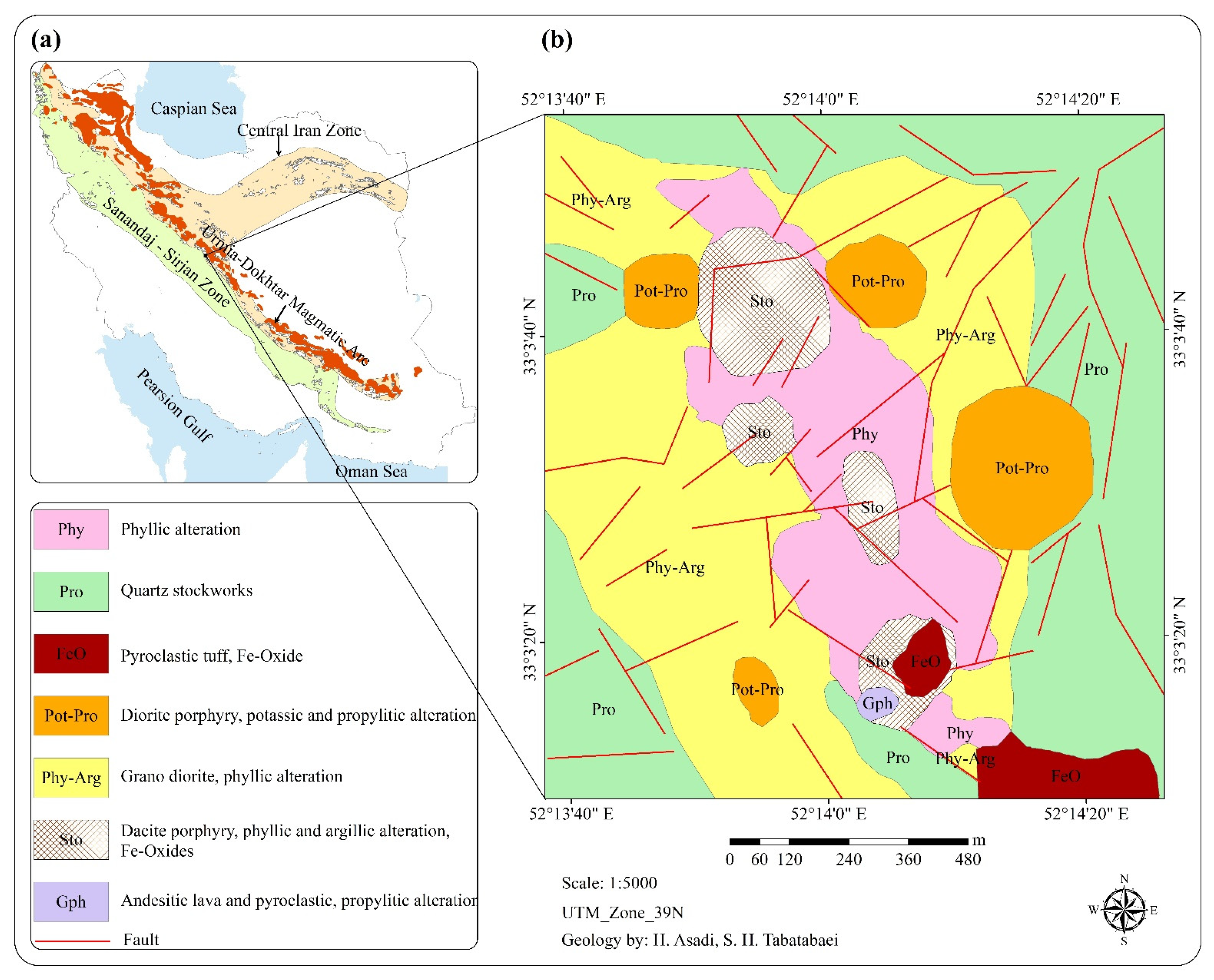
2. Geology of the Study Area
3. Materials and Methods
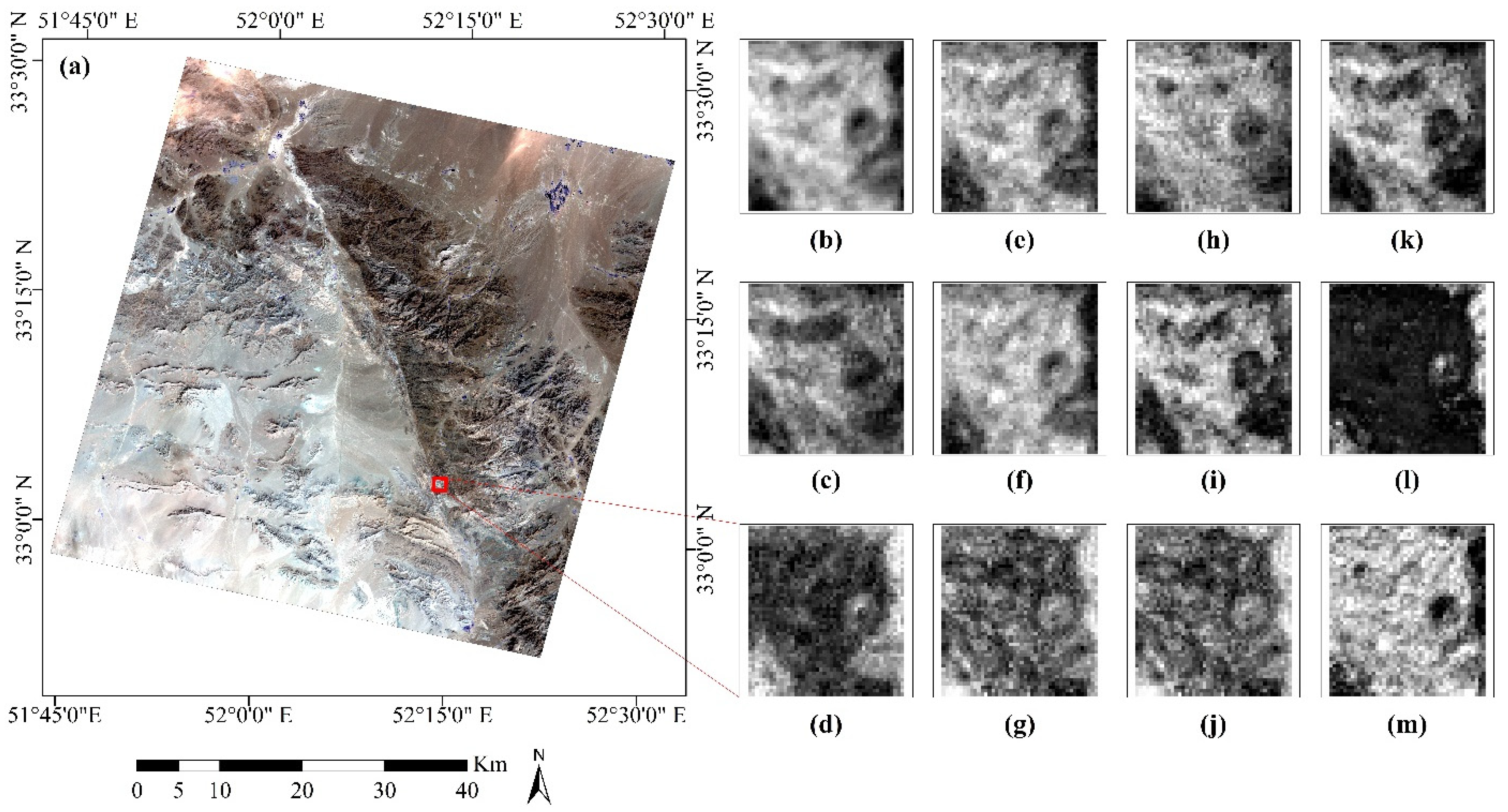
3.1. Data Characteristics
3.2. Methods
3.2.1. Dirichlet Process (DP)
3.2.2. Support Vector Machine (SVM)
3.2.3. Spectral Angle Mapper (SAM)
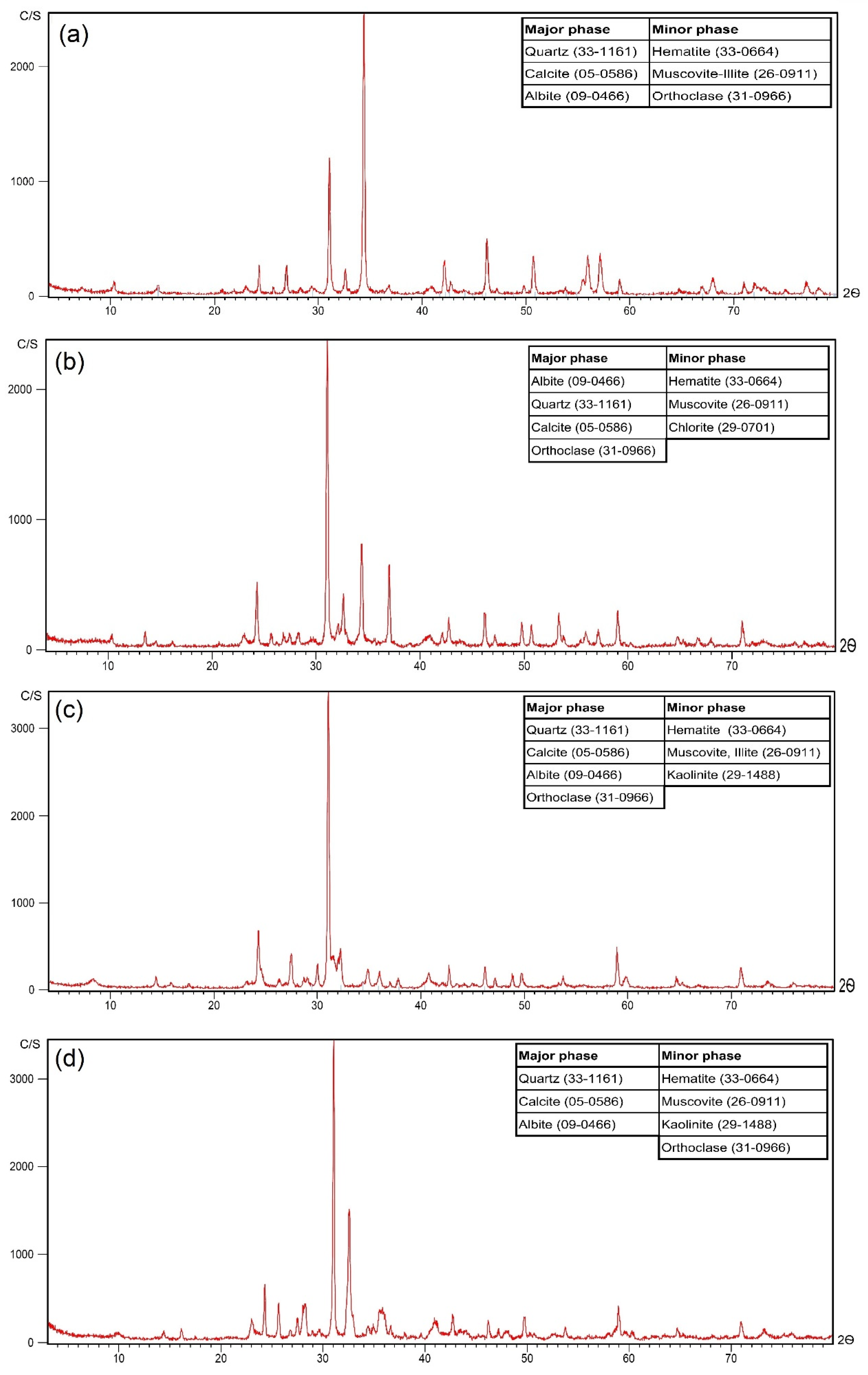
3.2.4. Laboratory Analysis
4. Results and Analysis
4.1. Determining the Training Data
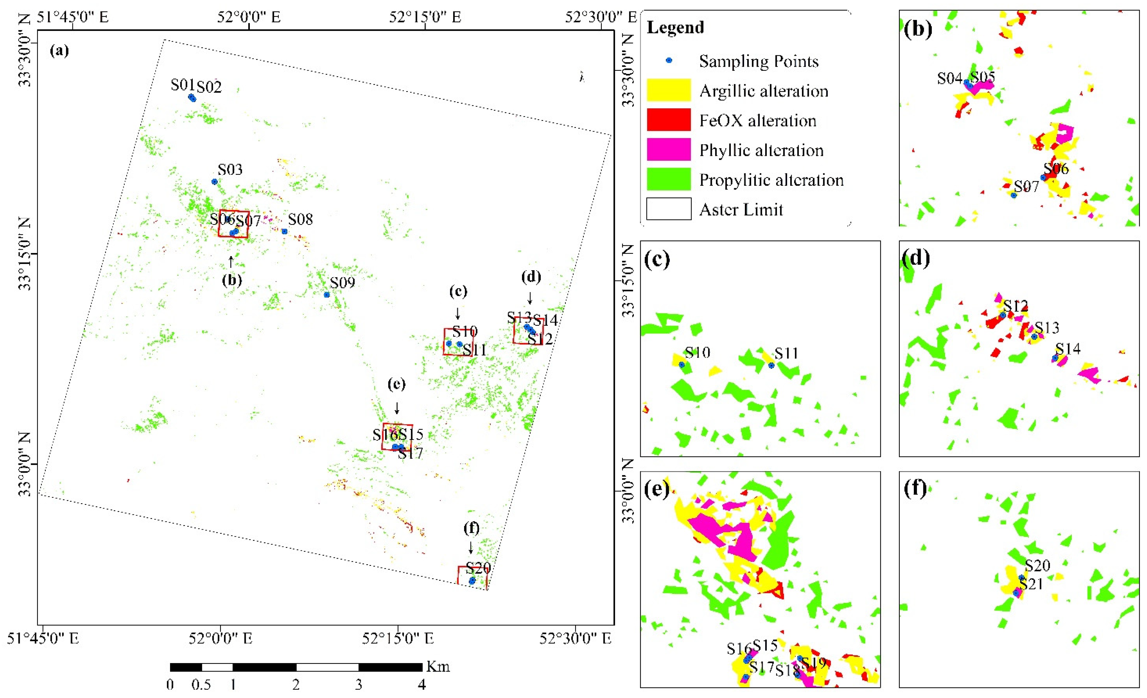
4.2. Detection of the Alteration Zones
4.3. Implementation of the DP Method on the Zeftreh Area
4.4. Implementation of the SVM on ASTER Data
4.5. Implementation of the SAM on ASTER Data
5. Fieldworks
5.1. Petrography Study
5.2. Geochemical Analysis
6. Accuracy Assessment
7. Discussion
8. Conclusions
Author Contributions
Funding
Data Availability Statement
Acknowledgments
Conflicts of Interest
Appendix A

| Row | Sample_NO | X (m) | Y (m) | Au (ppb) | Fe | Ag | As | Cu | Mn | Mo | Pb | Sb | Zn |
|---|---|---|---|---|---|---|---|---|---|---|---|---|---|
| 1 | S01 | 585,770 | 3,701,063 | <5 | 5855 | 0 | 8.3 | 18 | 178 | 2.1 | 5 | 1.08 | 20 |
| 2 | S02 | 586,064 | 3,700,766 | <5 | 17,302 | 0 | 8.9 | 5 | 29 | 5.3 | 5 | 1.24 | 53 |
| 3 | S03 | 589,488 | 3,690,065 | 70 | 13,866 | 0 | 150.7 | 15 | 219 | 6.8 | 63 | 201 | 39 |
| 4 | S04 | 591,489 | 3,685,219 | 104 | 185,397 | 0 | 289.2 | 467 | 161 | 20.9 | 86 | 1.1 | 138 |
| 5 | S05 | 591,544 | 3,685,158 | <5 | 21,278 | 0 | 9.1 | 6 | 67 | 2.18 | 6 | 1.29 | 16 |
| 6 | S06 | 592,703 | 3,683,705 | 7 | 123,344 | 0 | 8.9 | 112 | 564 | 4.8 | 32 | 1.09 | 1195 |
| 7 | S07 | 592,237 | 3,683,423 | <5 | 14,281 | 0 | 909.2 | 346 | 10,111 | 7.4 | 124 | 1.26 | 3014 |
| 8 | S08 | 599,089 | 3,684,040 | <5 | 8571 | 0.27 | 16.2 | 6 | 59 | 4 | 7 | 1.02 | 9 |
| 9 | S09 | 605,129 | 3,675,998 | 60 | 81,444 | 0.35 | 28.1 | 198 | 3464 | 2.27 | 32 | 1.17 | 60 |
| 10 | S10 | 621,599 | 3,670,515 | <5 | 35,705 | 0.27 | 8.8 | 16 | 110 | 3.4 | 7 | 1.13 | 78 |
| 11 | S11 | 623,023 | 3,670,502 | <5 | 47,093 | 0.22 | 8.9 | 63 | 1664 | 2.31 | 37 | 1.09 | 234 |
| 12 | S12 | 631,737 | 3,673,323 | <5 | 15,726 | 0.24 | 11.2 | 28 | 65 | 2.43 | 7 | 1.12 | 18 |
| 13 | S13 | 632,235 | 3,672,977 | <5 | 27,364 | 0.28 | 8.4 | 40 | 49 | 3.2 | 197 | 1.02 | 119 |
| 14 | S14 | 632,566 | 3,672,641 | 8 | 77,478 | 0.36 | 36.4 | 12 | 80 | 26.9 | 25 | 1.06 | 23 |
| 15 | S15 | 615,304 | 3,656,553 | 12 | 37,739 | 0.22 | 8.6 | 8 | 29 | 2.16 | 5 | 1.01 | 22 |
| 16 | S16 | 615,253 | 3,656,502 | 23 | 20,271 | 0.25 | 8.3 | 40 | 48 | 6.6 | 5 | 0.97 | 19 |
| 17 | S17 | 615,249 | 3,656,248 | 25 | 42,181 | 0.27 | 120.8 | 10 | 39 | 2.27 | 13 | 1.09 | 22 |
| 18 | S18 | 616,106 | 3,656,542 | 6 | 17,893 | 0.28 | 8.4 | 24 | 52 | 3.8 | 6 | 1.02 | 17 |
| 19 | S19 | 616,073 | 3,656,271 | <5 | 43,412 | 0.22 | 8.8 | 56 | 115 | 2.1 | 7 | 1.1 | 37 |
| 20 | S20 | 626,512 | 3,639,545 | <5 | 18,158 | 0 | 13 | 29 | 36 | 8.1 | 9 | 1.05 | 6 |
| 21 | S21 | 626,422 | 3,639,297 | 55 | 39,771 | 0 | 61.7 | 509 | 63 | 9.6 | 280 | 1.04 | 16 |
| Row | Sample_NO | SiO2 | Al2O3 | CaO | MgO | TiO2 | Fe2O3 | MnO | P2O5 | Na2O | K2O | SrO | L.O.I | Total |
|---|---|---|---|---|---|---|---|---|---|---|---|---|---|---|
| 1 | S01 | 56.24 | 24.19 | 0.71 | 0.66 | 0.75 | 3.14 | <0.1 | 0.48 | <0.1 | 2.24 | <0.1 | 10.70 | 99.11 |
| 2 | S02 | 49.23 | 22.81 | 2.70 | 1.55 | 0.85 | 6.08 | 0.14 | 0.46 | 1.54 | 3.23 | <0.1 | 10.00 | 98.60 |
| 3 | S03 | 41.85 | 20.15 | 8.97 | 2.94 | 0.61 | 6.81 | 0.28 | 0.38 | 0.32 | 2.23 | <0.1 | 13.50 | 98.04 |
| 4 | S04 | 50.16 | 23.24 | 5.66 | 1.58 | 0.43 | 3.43 | <0.1 | 0.32 | <0.1 | 1.94 | <0.1 | 11.30 | 98.06 |
| 5 | S05 | 47.91 | 23.51 | 6.90 | 1.64 | 0.43 | 4.01 | <0.1 | 0.34 | <0.1 | 2.81 | <0.1 | 11.49 | 99.03 |
| 6 | S06 | 43.86 | 22.51 | 6.31 | 1.39 | 0.65 | 7.35 | 0.17 | 0.31 | 0.62 | 2.91 | <0.1 | 12.62 | 98.70 |
| 7 | S07 | 53.06 | 18.94 | 4.31 | 3.26 | 0.71 | 6.49 | 0.26 | 0.42 | 3.68 | 3.58 | <0.1 | 4.14 | 98.85 |
| 8 | S08 | 43.38 | 18.91 | 8.87 | 2.86 | 0.66 | 6.80 | 0.16 | 0.43 | 1.99 | 2.22 | 0.12 | 12.70 | 99.08 |
| 9 | S09 | 52.32 | 22.22 | 5.02 | 2.14 | 0.50 | 2.44 | <0.1 | 0.34 | <0.1 | 3.85 | <0.1 | 9.50 | 98.33 |
| 10 | S10 | 41.42 | 17.01 | 8.66 | 3.44 | 0.77 | 9.28 | 0.33 | 0.57 | 2.56 | 1.85 | 0.10 | 12.98 | 98.98 |
| 11 | S11 | 44.85 | 21.87 | 4.79 | 2.21 | 0.62 | 7.67 | 0.15 | 0.36 | 0.65 | 3.27 | <0.1 | 12.34 | 98.77 |
| 12 | S12 | 49.31 | 19.29 | 5.46 | 2.63 | 0.55 | 6.14 | 0.15 | 0.38 | 2.33 | 2.46 | <0.1 | 9.39 | 98.09 |
| 13 | S13 | 48.28 | 17.41 | 8.81 | 3.28 | 0.69 | 8.44 | 0.18 | 0.52 | 2.97 | 3.62 | 0.19 | 5.15 | 99.56 |
| 14 | S14 | 44.26 | 17.00 | 6.57 | 3.07 | 0.75 | 8.95 | 0.17 | 0.37 | 2.91 | 3.70 | 0.10 | 9.84 | 97.69 |
| 15 | S15 | 56.24 | 24.19 | 0.71 | 0.66 | 0.75 | 3.14 | <0.1 | 0.48 | <0.1 | 2.24 | <0.1 | 6.70 | 95.11 |
| 16 | S16 | 49.23 | 22.81 | 2.70 | 1.55 | 0.85 | 6.08 | 0.14 | 0.46 | 1.54 | 3.23 | <0.1 | 10.00 | 98.60 |
| 17 | S17 | 41.85 | 20.15 | 8.97 | 2.94 | 0.61 | 6.81 | 0.28 | 0.38 | 0.32 | 2.23 | <0.1 | 13.50 | 98.04 |
| 18 | S18 | 50.16 | 23.24 | 5.66 | 1.58 | 0.43 | 3.43 | <0.1 | 0.32 | <0.1 | 1.94 | <0.1 | 11.30 | 98.06 |
| 19 | S19 | 47.91 | 23.51 | 6.90 | 1.64 | 0.43 | 4.01 | <0.1 | 0.34 | <0.1 | 2.81 | <0.1 | 11.49 | 99.03 |
| 20 | S20 | 43.86 | 22.51 | 6.31 | 1.39 | 0.65 | 7.35 | 0.17 | 0.31 | 0.62 | 2.91 | <0.1 | 12.62 | 98.70 |
| 21 | S21 | 53.06 | 18.94 | 4.31 | 3.26 | 0.71 | 6.49 | 0.26 | 0.42 | 3.68 | 3.58 | <0.1 | 4.14 | 98.85 |
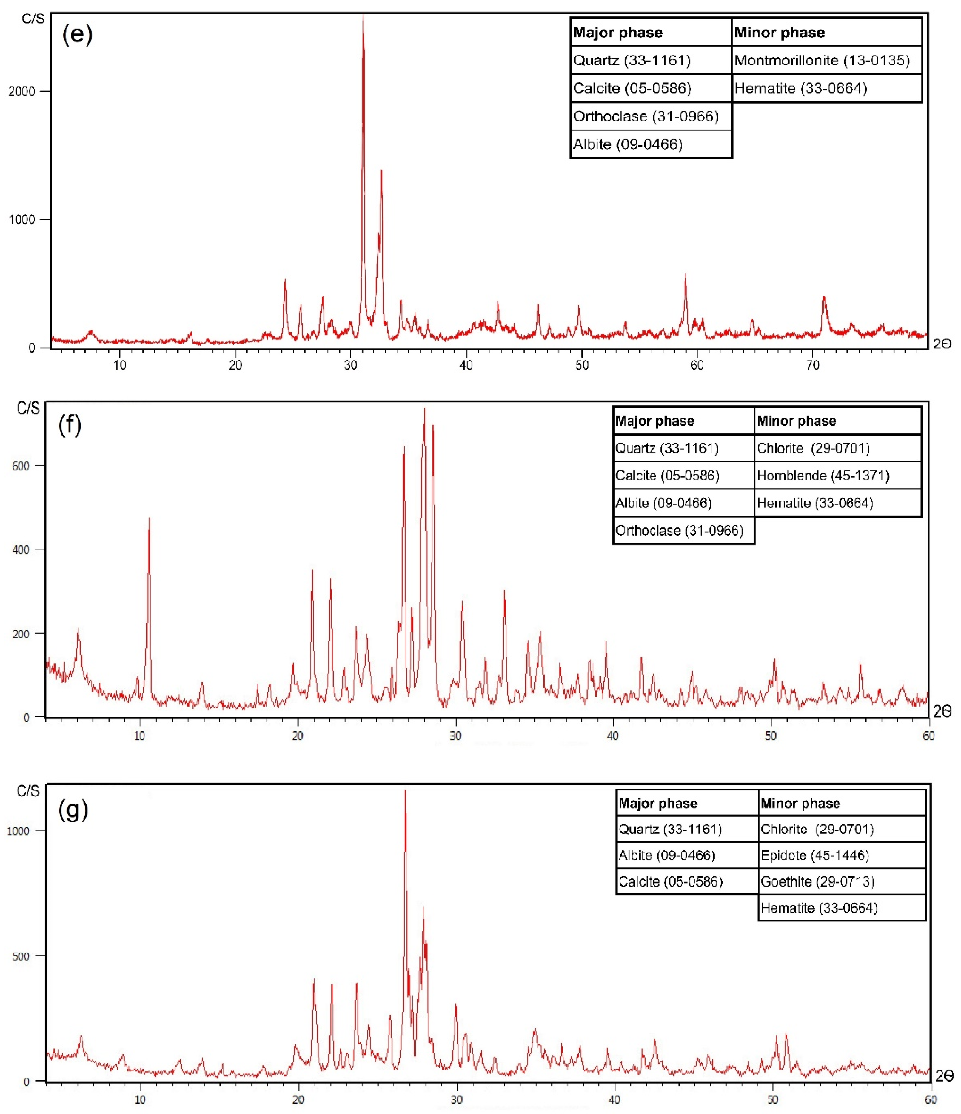
| Samples | Major Phase | Minor Phase | Alteration |
|---|---|---|---|
| S04 | Quartz, Calcite, Albite | Hematite, Muscovite, Illite, Orthoclase | Phyllic |
| S07 | Albite, Quartz, Calcite, Orthoclase | Hematite, Muscovite, Chlorite | Phyllic |
| S13 | Quartz, Calcite, Albite, Orthoclase | Hematite, Muscovite, Illite, Kaolinite | Phyllic–Argillic |
| S19 | Quartz, Calcite, Albite | Hematite, Muscovite, Kaolinite, Orthoclase | Phyllic–Argillic |
| S21 | Quartz, Calcite, Orthoclase, Albite | Montmorillonite, Hematite | Argillic |
| S14 | Quartz, Calcite, Albite, Orthoclase | Chlorite, Hornblende, Hematite | Propylitic |
| S16 | Quartz, Albite, Calcite | Chlorite, Epidote, Goethite, Hematite | Propylitic |
References
- El-Wahed, M.A.; Zoheir, B.; Pour, A.B.; Kamh, S. Shear-Related Gold Ores in the Wadi Hodein Shear Belt, South Eastern Desert of Egypt: Analysis of Remote Sensing, Field and Structural Data. Minerals 2021, 11, 474. [Google Scholar] [CrossRef]
- Krupnik, D.; Khan, S.D. High-Resolution Hyperspectral Mineral Mapping: Case Studies in the Edwards Limestone, Texas, USA and Sulfide-Rich Quartz Veins from the Ladakh Batholith, Northern Pakistan. Minerals 2020, 10, 967. [Google Scholar] [CrossRef]
- Ghezelbash, R.; Maghsoudi, A.; Carranza, E.J.M. Performance evaluation of RBF-and SVM-based machine learning algorithms for predictive mineral prospectivity modeling: Integration of SA multifractal model and mineralization controls. Earth Sci. Inform. 2019, 12, 277–293. [Google Scholar] [CrossRef]
- Cardoso-Fernandes, J.; Teodoro, A.C.; Lima, A.; Perrotta, M.; Roda-Robles, E. Detecting Lithium (Li) mineralizations from space: Current research and future perspectives. Appl. Sci. 2020, 10, 1785. [Google Scholar] [CrossRef] [Green Version]
- Peyghambari, S.; Zhang, Y. Hyperspectral remote sensing in lithological mapping, mineral exploration, and environmental geology: An updated review. J. Appl. Remote Sens. 2021, 15, 031501. [Google Scholar] [CrossRef]
- Hewson, R.; Mshiu, E.; Hecker, C.; van der Werff, H.; van Ruitenbeek, F.; Alkema, D.; van der Meer, F. The application of day and night time ASTER satellite imagery for geothermal and mineral mapping in East Africa. IJAEO 2020, 85, 101991. [Google Scholar] [CrossRef]
- Adiri, Z.; Lhissou, R.; El Harti, A.; Jellouli, A.; Chakouri, M. Recent advances in the use of public domain satellite imagery for mineral exploration: A review of Landsat-8 and Sentinel-2 applications. Ore Geol. Rev. 2020, 117, 103332. [Google Scholar] [CrossRef]
- Pour, A.B.; Hashim, M.; Hong, J.K.; Park, Y. Lithological and alteration mineral mapping in poorly exposed lithologies using Landsat-8 and ASTER satellite data: North-eastern Graham Land, Antarctic Peninsula. Ore Geol. Rev. 2019, 108, 112–133. [Google Scholar] [CrossRef]
- Pour, A.B.; Zoheir, B.; Pradhan, B.; Hashim, M. Editorial for the Special Issue: Multispectral and Hyperspectral Remote Sensing Data for Mineral Exploration and Environmental Monitoring of Mined Areas. Remote Sens. 2021, 13, 519. [Google Scholar] [CrossRef]
- Gupta, P.; Venkatesan, M. Mineral identification using unsupervised classification from hyperspectral data. In Emerging Research in Data Engineering Systems and Computer Communications; Springer: Berlin/Heidelberg, Germany, 2020; pp. 259–268. [Google Scholar]
- Pour, A.B.; Park, T.-Y.S.; Park, Y.; Hong, J.K.; Zoheir, B.; Pradhan, B.; Ayoobi, I.; Hashim, M. Application of multi-sensor satellite data for exploration of Zn–Pb sulfide mineralization in the Franklinian Basin, North Greenland. Remote Sens. 2018, 10, 1186. [Google Scholar] [CrossRef] [Green Version]
- Wylie, B.K.; Pastick, N.J.; Picotte, J.J.; Deering, C.A. Geospatial data mining for digital raster mapping. GISci. Remote Sens. 2019, 56, 406–429. [Google Scholar] [CrossRef]
- Dhingra, S.; Kumar, D. A review of remotely sensed satellite image classification. Int. J. Electr. Comput. Eng. 2019, 9, 1720–1731. [Google Scholar] [CrossRef]
- Gemusse, U.; Lima, A.; Teodoro, A. Comparing different techniques of satellite imagery classification to mineral mapping pegmatite of Muiane and Naipa: Mozambique. In Proceedings of the Earth Resources and Environmental Remote Sensing/GIS Applications X, Strasbourg, France, 10–12 September 2019; p. 111561E. [Google Scholar]
- Bachri, I.; Hakdaoui, M.; Raji, M.; Teodoro, A.C.; Benbouziane, A. Machine learning algorithms for automatic lithological mapping using remote sensing data: A case study from Souk Arbaa Sahel, Sidi Ifni Inlier, Western Anti-Atlas, Morocco. ISPRS Int. J. Geo-Inf. 2019, 8, 248. [Google Scholar] [CrossRef] [Green Version]
- Mojeddifar, S.; Mavadati, M. Integration of support vector machines for hydrothermal alteration mapping using ASTER data–case study: The northwestern part of the Kerman Cenozoic Magmatic Arc, Iran. Int. J. Min. Geo-Eng. 2020, 54, 45–50. [Google Scholar]
- Cardoso-Fernandes, J.; Teodoro, A.C.; Lima, A.; Roda-Robles, E. Semi-automatization of support vector machines to map lithium (Li) bearing pegmatites. Remote Sens. 2020, 12, 2319. [Google Scholar] [CrossRef]
- Reddy, C.K. Data Clustering: Algorithms and Applications; Chapman and Hall/CRC: London, UK, 2018. [Google Scholar]
- Abdi Jalebi, S.; Sharifzadeh, S.; Amiri, S. A New Method for Semi-Supervised Segmentation of Satellite Images. In Proceedings of the 2021 22nd IEEE International Conference on Industrial Technology (ICIT), Valencia, Spain, 10–12 March 2021; IEEE: New York, NY, USA, 2021. [Google Scholar]
- Saxena, A.; Prasad, M.; Gupta, A.; Bharill, N.; Patel, O.P.; Tiwari, A.; Er, M.J.; Ding, W.; Lin, C.-T. A review of clustering techniques and developments. Neurocomputing 2017, 267, 664–681. [Google Scholar] [CrossRef] [Green Version]
- Yang, M.-S.; Sinaga, K.P. A feature-reduction multi-view k-means clustering algorithm. IEEE Access 2019, 7, 114472–114486. [Google Scholar] [CrossRef]
- Ünlü, R.; Xanthopoulos, P. Estimating the number of clusters in a dataset via consensus clustering. Expert Syst. Appl. 2019, 125, 33–39. [Google Scholar] [CrossRef]
- Khosravi, M.; Rajabzadeh, M.A.; Qin, K.; Asadi, H.H. Tectonic setting and mineralization potential of the Zefreh porphyry Cu-Mo deposit, central Iran: Constraints from petrographic and geochemical data. J. Geochem. Explor. 2019, 199, 1–15. [Google Scholar] [CrossRef]
- Khosravi, M.; Christiansen, E.H.; Rajabzadeh, M.A. Chemistry of rock-forming silicate and sulfide minerals in the granitoids and volcanic rocks of the Zefreh porphyry Cu–Mo deposit, central Iran: Implications for crystallization, alteration, and mineralization potential. Ore Geol. Rev. 2021, 124, 104150. [Google Scholar] [CrossRef]
- Salehi, T.; Tangestani, M.H. Large-scale mapping of iron oxide and hydroxide minerals of Zefreh porphyry copper deposit, using Worldview-3 VNIR data in the Northeastern Isfahan, Iran. IJAEO 2018, 73, 156–169. [Google Scholar] [CrossRef]
- Abrams, M. The Advanced Spaceborne Thermal Emission and Reflection Radiometer (ASTER): Data products for the high spatial resolution imager on NASA’s Terra platform. IJRS 2000, 21, 847–859. [Google Scholar] [CrossRef]
- Guo, Y.-D.; Shi, Z. Characteristics and Applications of ASTER. Remote Sens. Technol. Appl. 2003, 5, 346–352. [Google Scholar]
- Erenoglu, R.C.; Arslan, N.; Erenoglu, O.; Arslan, E. Application of spectral analysis to determine geothermal anomalies in the Tuzla region, NW Turkey. Arab. J. Geosci. 2019, 12, 1–15. [Google Scholar] [CrossRef]
- Shawkya, M. Comparative Study of Atmospheric Correction Methods of ASTER Data to Enhance the Delineation of Uranium Mineralized Zones. Int. J. Intell. Comput. Inf. Sci. 2019, 19, 48–65. [Google Scholar] [CrossRef]
- Tucker, C.J. Red and photographic infrared linear combinations for monitoring vegetation. Remote Sens. Environ. 1979, 8, 127–150. [Google Scholar] [CrossRef] [Green Version]
- Ferguson, T.S. A Bayesian analysis of some nonparametric problems. Ann. Stat. 1973, 1, 209–230. [Google Scholar] [CrossRef]
- Escobar, M.D.; West, M. Bayesian density estimation and inference using mixtures. J. Am. Stat. Assoc. 1995, 90, 577–588. [Google Scholar] [CrossRef]
- Duan, J.A.; Guindani, M.; Gelfand, A.E. Generalized spatial Dirichlet process models. Biometrika 2007, 94, 809–825. [Google Scholar] [CrossRef] [Green Version]
- Ma, Z.; Lai, Y.; Kleijn, W.B.; Song, Y.-Z.; Wang, L.; Guo, J. Variational Bayesian learning for Dirichlet process mixture of inverted Dirichlet distributions in non-Gaussian image feature modeling. IEEE Trans. Neural Netw. Learn. Syst. 2018, 30, 449–463. [Google Scholar] [CrossRef]
- Teh, Y.W.; Jordan, M.I.; Beal, M.J.; Blei, D.M. Sharing clusters among related groups: Hierarchical Dirichlet processes. Adv. Neural Inf. Process. Syst. 2005, 17, 1385–1392. [Google Scholar]
- Vlachos, A.; Ghahramani, Z.; Korhonen, A. Dirichlet process mixture models for verb clustering. In Proceedings of the ICML Workshop on Prior Knowledge for Text and Language, Helsinki, Finland, 9 July 2008. [Google Scholar]
- Lugrin, T. Bayesian Semiparametrics for Modelling the Clustering of Extreme Values; École polytechnique fédérale de Lausanne: Écublens, Switzerland, 2013. [Google Scholar]
- Jain, A.; Murty, M.; Flynn, P.J. Data clustering: A review. ACM Comput. Surv. 2011, 31, 264–323. [Google Scholar] [CrossRef]
- Zuo, R.; Carranza, E.J.M. Support vector machine: A tool for mapping mineral prospectivity. Comput. Geosci. 2011, 37, 1967–1975. [Google Scholar] [CrossRef]
- Wang, K.; Cheng, L.; Yong, B. Spectral-similarity-based kernel of SVM for hyperspectral image classification. Remote Sens. 2020, 12, 2154. [Google Scholar] [CrossRef]
- Vapnik, V. The Nature of Statistical Learning Theory; Springer: New York, NY, USA, 1995; pp. 841–842. [Google Scholar]
- Ben-Hur, A.; Horn, D.; Siegelmann, H.T.; Vapnik, V. Support vector clustering. J. Mach. Learn. Res. 2001, 2, 125–137. [Google Scholar] [CrossRef]
- Bennett, K.; Demiriz, A. Semi-Supervised Support Vector Machines. Available online: https://proceedings.neurips.cc/paper/1998/file/b710915795b9e9c02cf10d6d2bdb688c-Paper.pdf (accessed on 24 March 2021).
- Widodo, A.; Yang, B.-S. Support vector machine in machine condition monitoring and fault diagnosis. MSSP 2007, 21, 2560–2574. [Google Scholar] [CrossRef]
- Wainer, J.; Fonseca, P. How to tune the RBF SVM hyperparameters? An empirical evaluation of 18 search algorithms. Artif. Intell. Rev. 2021, 54, 4771–4797. [Google Scholar] [CrossRef]
- Morales, R.; Wang, Y.; Zhang, Z. Unstructured point cloud surface denoising and decimation using distance RBF K-nearest neighbor kernel. In Proceedings of the Pacific-Rim Conference on Multimedia, Shanghai, China, 21–24 September 2010; pp. 214–225. [Google Scholar]
- Saljoughi, B.S.; Hezarkhani, A. A comparative analysis of artificial neural network (ANN), wavelet neural network (WNN), and support vector machine (SVM) data-driven models to mineral potential mapping for copper mineralizations in the Shahr-e-Babak region, Kerman, Iran. Appl. Geomat. 2018, 10, 229–256. [Google Scholar] [CrossRef]
- Khaleghi, M.; Ranjbar, H.; Shahabpour, J.; Honarmand, M. Spectral angle mapping, spectral information divergence, and principal component analysis of the ASTER SWIR data for exploration of porphyry copper mineralization in the Sarduiyeh area, Kerman province, Iran. Appl. Geomat. 2014, 6, 49–58. [Google Scholar] [CrossRef]
- Wang, M.; Huang, Z.; Zhang, X.; Zhang, Y.; Chen, M. Altered mineral mapping based on ground-airborne hyperspectral data and wavelet spectral angle mapper tri-training model: Case studies from Dehua-Youxi-Yongtai Ore District, Central Fujian, China. IJAEO 2021, 102, 102409. [Google Scholar]
- Choi, J.; Kim, G.; Park, N.; Park, H.; Choi, S. A hybrid pansharpening algorithm of VHR satellite images that employs injection gains based on NDVI to reduce computational costs. Remote Sens. 2017, 9, 976. [Google Scholar] [CrossRef] [Green Version]
- Renza, D.; Martinez, E.; Molina, I.J.A.i.S.R. Unsupervised change detection in a particular vegetation land cover type using spectral angle mapper. AdSpR 2017, 59, 2019–2031. [Google Scholar] [CrossRef]
- Wolf, R.E.; Adams, M. Multi-Elemental Analysis of Aqueous Geochemical Samples by Quadrupole Inductively Coupled Plasma-Mass Spectrometry (ICP-MS); US Department of the Interior, US Geological Survey: Washington, DC, USA, 2015.
- Monecke, T.; Köhler, S.; Kleeberg, R.; Herzig, P.M.; Gemmell, J.B. Quantitative phase-analysis by the Rietveld method using X-ray powder-diffraction data: Application to the study of alteration halos associated with volcanic-rock-hosted massive sulfide deposits. Can. Mineral. 2001, 39, 1617–1633. [Google Scholar] [CrossRef]
- Raith, M.M.; Raase, P. Thin Section Microscopy: A Comprehensive Guide. Available online: http://nationalpetrographic.com/thin-section-microscopy-a-comprehensive-guide.html (accessed on 24 March 2021).
- Pichler, H.; Schmitt-Riegraf, C. Rock-Forming Minerals in Thin Section; Springer Science & Business Media: Berlin, Germany, 1997. [Google Scholar]
- Chauhan, A.; Chauhan, P. Powder XRD technique and its applications in science and technology. J. Anal. Bioanal. Tech. 2014, 5, 1–5. [Google Scholar] [CrossRef] [Green Version]
- Rajendran, S.; Nasir, S. Characterization of ASTER spectral bands for mapping of alteration zones of volcanogenic massive sulphide deposits. Ore Geol. Rev. 2017, 88, 317–335. [Google Scholar] [CrossRef]
- Jain, R.; Sharma, R.U. Mapping of Mineral Zones using the Spectral Feature Fitting Method in Jahazpur belt, Rajasthan, India. Int. Res. J. Eng. Technol. (IRJET) 2018, 5, 562–567. [Google Scholar]
- Zoheir, B.; Emam, A.; Abdel-Wahed, M.; Soliman, N. Multispectral and radar data for the setting of gold mineralization in the South Eastern Desert, Egypt. Remote Sens. 2019, 11, 1450. [Google Scholar] [CrossRef] [Green Version]
- Chang, C.-I.; Cao, H.; Chen, S.; Shang, X.; Yu, C.; Song, M. Orthogonal subspace projection-based go-decomposition approach to finding low-rank and sparsity matrices for hyperspectral anomaly detection. ITGRS 2020, 59, 2403–2429. [Google Scholar] [CrossRef]
- Pour, A.B.; Hashim, M. Identification of hydrothermal alteration minerals for exploring of porphyry copper deposit using ASTER data, SE Iran. JAESc 2011, 42, 1309–1323. [Google Scholar] [CrossRef]
- Moghtaderi, A.; Moore, F.; Ranjbar, H. Application of ASTER and Landsat 8 imagery data and mathematical evaluation method in detecting iron minerals contamination in the Chadormalu iron mine area, central Iran. J. Appl. Remote Sens. 2017, 11, 016027. [Google Scholar] [CrossRef]
- Kokaly, R.; Clark, R.; Swayze, G.; Livo, K.; Hoefen, T.; Pearson, N.; Wise, R.; Benzel, W.; Lowers, H.; Driscoll, R. Usgs Spectral Library Version 7 Data: Us Geological Survey Data Release; United States Geological Survey (USGS): Reston, VA, USA, 2017.
- Sabins, F.F. Remote sensing for mineral exploration. Ore Geol. Rev. 1999, 14, 157–183. [Google Scholar] [CrossRef]
- Pour, A.B.; Sekandari, M.; Rahmani, O.; Crispini, L.; Läufer, A.; Park, Y.; Hong, J.K.; Pradhan, B.; Hashim, M.; Hossain, M.S. Identification of phyllosilicates in the antarctic environment using aster satellite data: Case study from the Mesa range, Campbell and Priestley glaciers, northern Victoria Land. Remote Sens. 2021, 13, 38. [Google Scholar] [CrossRef]
- Harsanyi, J.C.; Chang, C.-I. Hyperspectral image classification and dimensionality reduction: An orthogonal subspace projection approach. ITGRS 1994, 32, 779–785. [Google Scholar] [CrossRef] [Green Version]
- Gelfand, A.E.; Smith, A.F. Sampling-based approaches to calculating marginal densities. J. Am. Stat. Assoc. 1990, 85, 398–409. [Google Scholar] [CrossRef]
- Spiegelhalter, D.; Thomas, A.; Best, N.; Gilks, W. Bayesian Inference Using Gibbs Sampling Manual (Version ii) BUGS 0.5; MRC Biostatistics Unit, Institute of Public Health: Cambridge, UK, 1996; p. 59. [Google Scholar]
- Spiegelhalter, D.; Thomas, A.; Best, N.; Lunn, D. WinBUGS User Manual. 2003. Available online: https://www.mrc-bsu.cam.ac.uk/wp-content/uploads/manual14.pdf (accessed on 27 February 2021).
- Foody, G.M. Explaining the unsuitability of the kappa coefficient in the assessment and comparison of the accuracy of thematic maps obtained by image classification. Remote Sens. Environ. 2020, 239, 111630. [Google Scholar] [CrossRef]
- Congalton, R.G. A review of assessing the accuracy of classifications of remotely sensed data. Remote Sens. Environ. 1991, 37, 35–46. [Google Scholar] [CrossRef]
- Mathieu, L. Quantifying hydrothermal alteration: A review of methods. Geosciences 2018, 8, 245. [Google Scholar] [CrossRef] [Green Version]
- Frutuoso, R.; Lima, A.; Teodoro, A.C. Application of remote sensing data in gold exploration: Targeting hydrothermal alteration using Landsat 8 imagery in northern Portugal. Arab. J. Geosci. 2021, 14, 1–18. [Google Scholar] [CrossRef]
- Chattoraj, S.L.; Prasad, G.; Sharma, R.U.; van der Meer, F.D.; Guha, A.; Pour, A.B. Integration of remote sensing, gravity and geochemical data for exploration of Cu-mineralization in Alwar basin, Rajasthan, India. IJAEO 2020, 91, 102162. [Google Scholar] [CrossRef]
- Pour, A.B.; Park, T.-Y.S.; Park, Y.; Hong, J.K.; Muslim, A.M.; Läufer, A.; Crispini, L.; Pradhan, B.; Zoheir, B.; Rahmani, O.; et al. Landsat-8, advanced spaceborne thermal emission and reflection radiometer, and WorldView-3 multispectral satellite imagery for prospecting copper-gold mineralization in the northeastern Inglefield Mobile Belt (IMB), northwest Greenland. Remote Sens. 2019, 11, 2430. [Google Scholar] [CrossRef] [Green Version]
- Shirmard, H.; Farahbakhsh, E.; Pour, A.B.; Muslim, A.M.; Müller, R.D.; Chandra, R. Integration of Selective Dimensionality Reduction Techniques for Mineral Exploration Using ASTER Satellite Data. Remote Sens. 2020, 12, 1261. [Google Scholar] [CrossRef] [Green Version]
- Sekandari, M.; Masoumi, I.; Pour, A.B.; Muslim, A.M.; Rahmani, O.; Hashim, M.; Zoheir, B.; Pradhan, B.; Misra, A.; Aminpour, S.M. Application of Landsat-8, Sentinel-2, ASTER and WorldView-3 Spectral Imagery for Exploration of Carbonate-Hosted Pb-Zn Deposits in the Central Iranian Terrane (CIT). Remote Sens. 2020, 12, 1239. [Google Scholar] [CrossRef] [Green Version]
- Parsa, M.; Pour, A.B. A simulation-based framework for modulating the effects of subjectivity in greenfields’ Mineral Prospectivity Mapping with geochemical and geological data. J. Geochem. Explor. 2021, 229, 106838. [Google Scholar] [CrossRef]
- Bolouki, S.M.; Ramazi, H.R.; Maghsoudi, A.; Beiranvand Pour, A.; Sohrabi, G. A remote sensing-based application of bayesian networks for epithermal gold potential mapping in Ahar-Arasbaran area, NW Iran. Remote Sens. 2020, 12, 105. [Google Scholar] [CrossRef] [Green Version]
- Parsa, M. A data augmentation approach to XGboost-based mineral potential mapping: An example of carbonate-hosted Zn-Pb mineral systems of Western Iran. J. Geochem. Explor. 2021, 228, 106811. [Google Scholar] [CrossRef]


| Classes | Phyllic | Argillic | Propylitic | Fe-Oxides | Total | User’s Accuracy |
|---|---|---|---|---|---|---|
| Unclassified | 20 | 46 | 9 | 30 | 105 | |
| Phyllic | 172 | 23 | 0 | 0 | 195 | 88.21 |
| Argillic | 33 | 795 | 6 | 47 | 881 | 90.24 |
| Propylitic | 0 | 3 | 201 | 1 | 205 | 98.05 |
| Fe-Oxides | 0 | 17 | 0 | 104 | 121 | 85.95 |
| Total | 225 | 884 | 216 | 182 | 1507 | |
| Producer’s accuracy | 76.44 | 89.93 | 93.06 | 57.14 | ||
| Overall accuracy | 84.4 | |||||
| Kappa coefficient | 0.744 |
| Classes | Phyllic | Argillic | Propylitic | Fe-Oxides | Total | User’s Accuracy |
|---|---|---|---|---|---|---|
| Unclassified | 8 | 102 | 47 | 23 | 180 | |
| Phyllic | 146 | 107 | 0 | 7 | 260 | 56.15 |
| Argillic | 43 | 586 | 0 | 15 | 644 | 90.99 |
| Propylitic | 0 | 1 | 128 | 0 | 129 | 99.22 |
| Fe-Oxides | 24 | 108 | 9 | 153 | 294 | 52.04 |
| Total | 221 | 904 | 184 | 198 | 1507 | |
| Producer’s accuracy | 66.06 | 64.82 | 69.57 | 77.27 | ||
| Overall accuracy | 67.2 | |||||
| Kappa coefficient | 0.52 |
Publisher’s Note: MDPI stays neutral with regard to jurisdictional claims in published maps and institutional affiliations. |
© 2021 by the authors. Licensee MDPI, Basel, Switzerland. This article is an open access article distributed under the terms and conditions of the Creative Commons Attribution (CC BY) license (https://creativecommons.org/licenses/by/4.0/).
Share and Cite
Yousefi, M.; Tabatabaei, S.H.; Rikhtehgaran, R.; Pour, A.B.; Pradhan, B. Application of Dirichlet Process and Support Vector Machine Techniques for Mapping Alteration Zones Associated with Porphyry Copper Deposit Using ASTER Remote Sensing Imagery. Minerals 2021, 11, 1235. https://doi.org/10.3390/min11111235
Yousefi M, Tabatabaei SH, Rikhtehgaran R, Pour AB, Pradhan B. Application of Dirichlet Process and Support Vector Machine Techniques for Mapping Alteration Zones Associated with Porphyry Copper Deposit Using ASTER Remote Sensing Imagery. Minerals. 2021; 11(11):1235. https://doi.org/10.3390/min11111235
Chicago/Turabian StyleYousefi, Mastoureh, Seyed Hassan Tabatabaei, Reyhaneh Rikhtehgaran, Amin Beiranvand Pour, and Biswajeet Pradhan. 2021. "Application of Dirichlet Process and Support Vector Machine Techniques for Mapping Alteration Zones Associated with Porphyry Copper Deposit Using ASTER Remote Sensing Imagery" Minerals 11, no. 11: 1235. https://doi.org/10.3390/min11111235
APA StyleYousefi, M., Tabatabaei, S. H., Rikhtehgaran, R., Pour, A. B., & Pradhan, B. (2021). Application of Dirichlet Process and Support Vector Machine Techniques for Mapping Alteration Zones Associated with Porphyry Copper Deposit Using ASTER Remote Sensing Imagery. Minerals, 11(11), 1235. https://doi.org/10.3390/min11111235