Common Problems and Pitfalls in Fluid Inclusion Study: A Review and Discussion

Abstract

The study of fluid inclusions is important for understanding various geologic processes involving geofluids. However, there are a number of problems that are frequently encountered in the study of fluid inclusions, especially by beginners, and many of these problems are critical for the validity of the fluid inclusion data and their interpretations. This paper discusses some of the most common problems and/or pitfalls, including those related to fluid inclusion petrography, metastability, fluid phase relationships, fluid temperature and pressure calculation and interpretation, bulk fluid inclusion analysis, and data presentation. A total of 16 problems, many of which have been discussed in the literature, are described and analyzed systematically. The causes of the problems, their potential impact on data quality and interpretation, as well as possible remediation or alleviation, are discussed.

1. Introduction

Geofluids play an important role in most geologic processes, from molecular-scale fluid-rock reaction to global tectonics. Because fluid inclusions entrapped in minerals formed in various geologic settings are the actual samples of the paleo-geofluids, they can provide indispensable information about the environments and geologic processes in which the minerals were formed, particularly the composition, temperature and pressure of the geofluids [1,2,3,4,5,6,7,8]. Indeed, since the pioneer work by Sorby (1858) [1], the study of fluid inclusions has gradually become an important sub-discipline in geoscience, and fluid inclusions have been applied to the study of various geologic processes, including magmatic, hydrothermal, metamorphic, sedimentary and structural, in environments ranging from high pressure–high temperature conditions in the mantle to low pressure–low temperature conditions on the Earth’s surface [5]. Fluid inclusions are particularly widely applied to the study of mineral deposits [3,9,10,11]. For example, it has been shown that the percentage of papers containing fluid inclusion studies published in Economic Geology between 1970 and 2010 ranges from 5% to 27% on a yearly basis [12]. The majority of problems related to fluid inclusion study discussed in this paper are derived from studies of mineral deposits, but most of them are also encountered in other fields such as diagenesis and oil-gas reservoirs in sedimentary basins.

Because the study of fluid inclusions deals with the composition, pressure and temperature of geofluids, it is often considered as a geochemical method. For example, fluid inclusion study constitutes a chapter in the book Geochemistry of Hydrothermal Ore Deposits [9] and also in Treatise on Geochemistry [11]. However, unlike most geochemical methods which are meant to yield reproducible results within analytical uncertainties, the study of fluid inclusions may potentially result in significantly different results by different researchers depending on the approaches and procedures used in the study. This is obviously a problem in scientific research: if the results depend on the researchers and are not reproducible, the validity of the data are questionable. There are multiple steps in fluid inclusion studies in which things may go wrong, but most of these problems can be avoided if certain rules are followed. The primary purpose of this paper is therefore to point out where problems most likely occur, based on published papers in the literature and our experiences in research, teaching, paper reviewing and editing. For each problem, we will analyze the reasons why things may go wrong and what the consequences may be, and finally we will offer some recommendations about how to approach the problems and what precautions need to be taken.

Most of the problems and/or pitfalls have been repeatedly discussed elsewhere [3,9,10,13,14,15], but the discussions are generally dispersed in the literature and the problems persist. This paper therefore represents an effort to increase the awareness of these problems by consolidating them together and analyzing them systematically. Many of the problems are fairly straightforward and may appear simple to experienced fluid inclusionists, however they remain common hurdles for beginners of fluid inclusion study, and therefore it is still important to point them out and discuss them. Other problems may not be so obvious, and the understanding of the problems and the approaches to treat them may be controversial. It must be pointed out, however, that it is not our intention to discuss all problems in all aspects of fluid inclusion studies. For example, detailed technical problems in fluid inclusion analysis such as LA-ICP-MS [16] or Raman spectroscopy [17] are not discussed in this paper. Difficulty and errors associated with fluid PVTX calculations that are related to uncertainties in fluid phase proportion estimation, choice of a representative chemical system, and appropriate equation of state, are not discussed in any detail either. Furthermore, although melt inclusions can be considered as a type of fluid inclusion, problems particular to melt inclusion studies are not discussed in this paper either. No attempt has been made to either trace where the problems/pitfalls were initially derived from or to comment on individual studies. The main purpose of this paper is to help beginners of fluid inclusion study avoid some common mistakes and minimize the impact that may be caused by invalid data and/or incorrect interpretations.

2. Problems Related to Fluid Inclusion Petrography

2.1. Problem #1: Study of Fluid Inclusions without Determining the Paragenetic Position of the Host Mineral

In order to conduct a meaningful study of fluid inclusions, it is essential to know the relative timing of the minerals that host the fluid inclusions, or the paragenetic positions of the minerals in the rocks being studied [3,10]. Unfortunately, it is not uncommon to see beginners jump to study fluid inclusions in a sample without knowing the paragenesis of the minerals. For example, when given an ore sample that contains both ore minerals and quartz, an unexperienced student may go straight to study fluid inclusions in the quartz with an aim to characterize the ore-forming fluid, even though the quartz may have been formed before or after the ore minerals and therefore is unrelated to the ore-forming fluid. Therefore, it is essential to establish the paragenetic sequence based on detailed observations in the field and on hand samples as well as petrographic work of thin sections, before any fluid inclusion work is conducted.

This is particularly important if the purpose of the fluid inclusion study is to evaluate the evolution of the fluid system before, during and after mineralization. For example, in the sample shown in Figure 1, bladed calcite cementing limestone fragments was formed before mineralization, and sphalerite cementing fragments that have already been cemented by bladed calcite represents an ore-stage product, whereas the anhedral calcite filling residual pore left by sphalerite was likely formed after mineralization. A systematic study of fluid inclusions in the bladed calcite, sphalerite and anhedral calcite would reveal the evolution of the fluid system from pre-mineralization through syn-mineralization to post-mineralization stages. Conversely, if fluid inclusions in the bladed calcite were taken to represent ore-forming fluids simply because the sample is an ore, wrong conclusions about the mineralization fluids and P–T conditions will be made.

2.2. Problem #2: Assigning Fluid Inclusions as “Primary” without Describing Their Actual Mode of Occurrence

The fluid inclusions in a mineral may be divided according to their trapping mechanisms into three genetic types with respect to the genesis of the host crystal, i.e., primary inclusions, secondary inclusions and pseudosecondary inclusions [3,15,18,19]. Primary inclusions were entrapped on the growing face of the host crystal during its precipitation, and secondary inclusions were entrapped in crosscutting fractures after the formation of the host mineral, whereas pseudosecondary inclusions were entrapped in fractures during crystal growth (i.e., they are overgrown by a layer of the host crystal). Although this classification of fluid inclusions is well defined and is essential in the interpretation of fluid inclusion data, in practice it is generally difficult to determine if a fluid inclusion is primary, secondary, or pseudosecondary. In fact, it is prudent to acknowledge that not all fluid inclusions can be assigned definitively to one of the three genetic types, as petrographic relationships in a given sample may simply be ambiguous.

Roedder (1984; pages 43–45) [3] proposed some general guidelines for discriminating the three types of inclusions, which have been widely used in fluid inclusion studies. Unfortunately, although what were proposed by Roedder (1984) [3] as “criteria” for a certain type of fluid inclusion are merely some possibilities, they have been often used as definite “rules”. In fact, Roedder (1984) [3] explicitly pointed out that some of the criteria that he listed are not conclusive. For example, negative crystal shape of fluid inclusions may indicate a primary origin, but in many cases, secondary inclusions have negative crystal shape [19], as clearly exemplified by the secondary inclusions crosscutting growth zones in the cassiterite crystal shown in Figure 2a. Therefore, ‘negative crystal shape’ cannot be used as a diagnostic criterion for primary inclusions. However, shapes and sizes are nevertheless worth recording. Besides enhancing the characterization of the generation of inclusions being studied, shapes and sizes may help to explain unusual analytical results (e.g., small, flat liquid inclusions often do not nucleate a bubble upon cooling; phase transitions may be obscured when viewed down the long axis of elongate inclusions), and they can yield information about the post-entrapment history of the sample [20,21].

If one reads the entire list of criteria by Roedder (1984) [3] and puts them into context, it becomes clear that, even though it is not directly pointed out by Roedder (1984) [3], most of the “criteria” should be used as general guides rather than evidence. In other words, fluid inclusions satisfying most of Roedder’s (1984) [3] criteria for primary origin are only possibly, not definitely, primary inclusions. To conclude that a fluid inclusion assemblage is primary, the inclusions in the assemblage must be related to a feature that reflects entrapment during growth of the host crystal, or define such a feature. As a result of not fully recognizing the complexity and potential ambiguity of fluid inclusion classification, many beginners simply assign a fluid inclusion to be primary, secondary or pseudosecondary in the early stage of fluid inclusion study (i.e., petrography) and then continue to label them as such throughout the study. Obviously, mis-identification of secondary fluid inclusions as primary fluid inclusions, or vice versa, may lead to serious problems in the interpretation of the fluid inclusion data.

Assignment of inclusions to primary, secondary or pseudosecondary types clearly involves interpretation. In order to minimize the negative consequence of mis-assigning a fluid inclusion using ambiguous criteria as discussed above, it is strongly recommended to describe the observations on which the interpretation is based at the stage of petrographic study. For example, in the case shown in Figure 2b, instead of simply labeling the inclusions in the cloudy core as primary inclusions, describe them as ‘randomly (and densely) distributed within the core of a quartz crystal’. Indeed, considering that the cloudy core is overprinted by several microfractures, it is difficult to say if a given inclusion in the cloudy core is definitely primary, although this may be true for the majority. Similarly, those occurring in the relatively clean rim should be described as ‘isolated’, ‘cluster’, ‘intra-crystal trail’ or ‘inter-crystal trail’ (Figure 2b), rather than simply labelled as primary, pseudosecondary or secondary. This is also important from the point of view of data recording: if a fluid inclusion is simply recorded as a “primary inclusion”, it will be impossible for someone else (or even the author him/herself, after certain time) to know exactly how the inclusion occurs, and thus impossible to later re-interpret it as a secondary inclusion even if new petrographic evidence (e.g., from cathodoluminescence imaging) later becomes available.

Putting the above recommendations into practice, recording the petrographic features of fluid inclusions is aided by using a checklist with fields labelled “textural setting” and “genetic type”. In the former, one of the terms ‘isolated’, ‘cluster’, ‘intra-crystal trail’ or ‘inter-crystal trail’ can be entered. In the latter, one of the four genetic types can be entered: primary, secondary, pseudosecondary or “undetermined”.

2.3. Problem #3: Non-Use and Misuse of the ‘Fluid Inclusion Assemblage’ (FIA) Concept

A ‘fluid inclusion assemblage’ (FIA) [22] is defined by Goldstein and Reynolds (1994) [14] and Goldstein (2001) [15] as the most finely discriminated, petrographically distinguishable group of fluid inclusions formed by a single event of fluid inclusion entrapment. Since its emergence, the fluid inclusion assemblage (FIA) concept has been increasingly appreciated and used in the fluid inclusion community (e.g., [23,24,25]). This is largely due to its usefulness in validating fluid inclusion data as imposed by Roedder’s rules [19]: (1) the individual inclusions trapped a single (i.e., homogeneous) phase; (2) the inclusions represent an isochoric (constant volume) system; and (3) after trapping, nothing has been added to, or removed from, the inclusions. However, there are still many publications on fluid inclusions in the literature that do not use the FIA concept, which result in poorly constrained fluid inclusion data. On the other hand, when the FIA concept is used, there are also various misunderstandings, as discussed below. It should be noted that an equivalent term, ‘group of synchronous inclusions’, is used by some authors [26]. To avoid confusion, this paper uses only the term ‘fluid inclusion assemblage’.

One misunderstanding of FIA is to treat it as the co-occurrence of different types (compositional or phase assemblage) of fluid inclusions that are interpreted to be of the same generation (e.g., primary) in the same host mineral. Thus, in the schematic example shown in Figure 3, the occurrence of three types of fluid inclusions (L-only, L-dominated and V-dominated) interpreted as primary inclusions may be referred to as one FIA, which obviously does not comply with the definition of FIA by Goldstein and Reynolds (1994) [14]. According to Goldstein and Reynolds (1994) [14], there are up to nine FIAs (note the single isolated inclusion (#8) is not considered as an FIA) in Figure 3, not just one or two.

A second misunderstanding is that “groups of fluid inclusions with similar vapor/liquid ratios can be considered as an FIA regardless if there is petrographic evidence indicating they were trapped synchronously”. Thus, group 3 and group 5 in Figure 3 represent two individual FIAs, but they cannot be considered together as one FIA even though the fluid inclusions all have similar vapor/liquid ratios. Similarly, the fluid inclusions in group 6 may not be considered as one FIA simply because they have similar vapor/liquid ratios; they may constitute an FIA only if they can be demonstrated to be coeval, e.g., pseudosecondary, secondary, or primary on a growth zone oriented oblique to the cut of the crystal.

A third misunderstanding is that “only a group of fluid inclusions with consistent vapor/liquid ratios can be considered as an FIA, and those with different vapor/liquid ratios cannot be treated as an FIA, because the variation of vapor/liquid ratios suggests that they were not entrapped at the same time, which is contradictory with the definition of FIAs”. According to this understanding, groups 1, 3, 5, 6 and 9 in Figure 3 are FIAs, whereas groups 2, 4, 7 and 10 are not FIAs. This understanding contradicts the definition of FIA, in which the synchronous formation of the fluid inclusions is interpreted from petrographic evidence rather than from consistency of phase ratios. In fact, the consistency of phase ratios (and microthermometric data) should be used to evaluate whether or not a single phase was entrapped, rather than to judge if the inclusions were entrapped at the same time. Thus, groups #1–5, 9 and 10 in Figure 3 are all FIAs, although some of them (#1, 3, 5, 9) may have resulted from homogeneous trapping and may be termed “good FIAs” (in the sense that they satisfy Roedder’s rules), whereas others (#2, 4, and perhaps #10) may have resulted from heterogeneous trapping or post-entrapment modification and may be termed “bad FIAs” (in the sense that they do not satisfy Roedder’s rules). It should be pointed out that the so-called “bad FIAs” means that the microthermometric data from the majority of these inclusions are invalid; it does not mean that they are useless. In fact, some of the inclusions in the “bad FIAs”, particularly those with the lowest homogenization temperatures, may still provide valid microthermometric data, and heterogeneous trapping reflected by them actually provides the best evidence for fluid immiscibility, as discussed later in Problem #9.

In addition to the above misunderstandings about FIAs, there are a few problems related to the use of FIA that are worth further discussion. Fluid inclusions that cannot be unambiguously determined to be entrapped contemporaneously, such as those in the cloudy core in Figure 2b, or groups 6 and 7 in Figure 3, cannot be counted as FIAs. In the cases of randomly distributed fluid inclusions (cloudy core in Figure 2b), although most of the inclusions may be primary, they are unlikely to all have been contemporaneously entrapped. In the cases of fluid inclusion clusters (groups 6 and 7 in Figure 3), they may be contemporaneously entrapped if they are pseudosecondary or secondary, but are unlikely to be contemporaneous if they are primary. In these cases, forcing the groups of inclusions into individual FIAs may result in unjustified rejection of microthermometric data if Goldstein and Reynolds’s (1994) [14] criteria of consistency (e.g., variation of homogenization temperatures <15 ℃ within an FIA) are strictly applied.

Nevertheless, the FIA concept may still be applied to the non-FIAs or “quasi-FIAs” to constrain the microthermometric data, although in a less strict sense. Thus, if the microthermometric data are more or less consistent within a cluster (group 6 in Figure 3, which may not be an FIA), the fluid inclusions likely did not result from heterogeneous trapping or experience significant post-entrapment modification, and the data may be considered acceptable. Conversely, if the data are very inconsistent within a cluster (group 7 in Figure 3), the fluid inclusions may have been entrapped at different times (e.g., unrecognized secondary inclusions overprinting primary inclusions), resulted from heterogeneous trapping, or experienced necking down or other forms of significant post-entrapment modification such as stretching, and the data are unusable [27]. The worst thing for one to do, which is not uncommon among beginners, is to measure all the fluid inclusions in situations like group 7 in Figure 3, without considering the inconsistency of microthermometric data and potential causes. A safe way to deal with the situations like group 7 in Figure 3 is to skip this group of inclusions, i.e., do not measure any of them, unless the objective of study is to assess the effect of post-entrapment modification or other particular geologic processes related to it.

There is no doubt that application of the FIA concept has improved the rigor and objectivity with which the phase state of natural fluids can be identified from fluid inclusion studies. On the other hand, there is no doubt that prior to the definition of the FIA concept there were a wealth of valuable and accurate fluid inclusion studies conducted—which have greatly contributed to various fields of earth science. One could argue that it is not really necessary to use the FIA concept. However, many of the fluid inclusion works prior to the FIA era actually followed its principles without explicitly mentioning it, as exemplified by the study of fluid inclusions in individual growth zones in sphalerite from the Creede epithermal vein system [28]. Thus, if fluid inclusion homogenization temperatures from 100 to 400 °C were obtained for the fluid inclusions in group 7 in Figure 3, an experienced fluid inclusionist would reject the bulk of the data even without using the FIA concept. Conversely, a blunt beginner might accept all the data without critical thinking and would come to wrong conclusions about the fluid temperature (e.g., using the range of homogenization temperatures to indicate real temperature variation). However, if the FIA concept is systematically applied as a formal approach, such mistakes can be avoided.

3. Problems Related to Metastability

Metastability refers to the occurrence of any combination of phases that has a higher free energy than the most stable or equilibrium combination. The metastable phenomena most commonly encountered in fluid inclusion studies are due to the failure of a stable phase (solid, vapor or liquid) to nucleate upon cooling in nature or in the laboratory. For example, pure water is supposed to be frozen below 0 °C, but in actual microthermometric cooling runs, extra cooling to lower than –30 °C is typically required to freeze a pure water inclusion. Although some of the metastable phenomena may be useful, e.g., the cycling technique that makes use of metastability to accurately and precisely measure melting temperatures and liquid-vapor homogenization temperatures [3,14,29,30], metastability can cause problems, and some of the common ones are discussed below.

3.1. Problem #4: Misunderstanding of the Nature of First Melting and Misuse of ‘Eutectic Temperature’

It is well understood that fluids containing different components have different eutectic temperatures, which represent the lowest temperature at which the first melting of a solid phase occurs. For example, the eutectic temperature for the H₂O-NaCl system is –21.2 °C and that for the H₂O-NaCl-CaCl₂ system is –52 °C [31]. Conversely, the eutectic temperature can be used to infer the chemical components in a fluid inclusion. However, it is often ignored that the eutectic temperatures only apply to equilibrium situations, even though metastable phase changes are far more common than equilibrium ones with respect to first melting. In fact, experiments with synthetic fluid inclusions of the H₂O-NaCl-CaCl₂ system that couple the heating-freezing stage with Raman spectroscopy reveal that the majority of the fluid inclusions contain significant amounts of liquid along with some solids when cooled to –185 °C, and this situation persists regardless of the cooling rate and duration [32,33,34]. This means that many fluid inclusions that appear frozen are not completely frozen, and therefore what may appear to be first melting during warming is actually some other process, such as coarsening of crystal grains [32,34,35]. Although it is difficult to determine the exact nature of the apparent “first melting”, it is most likely not eutectic melting, and therefore, it is not recommended to use the term ‘eutectic temperature’ (often abbreviated as T_e in the literature) to describe the temperature of this event. Instead, it is recommended to use “first melting temperature” (or T_fm), or “apparent eutectic temperature” (T_e*) as this term is observational (or apparently observational) rather than theoretical (for T_e). It follows that using the first melting temperature to infer the components of the fluid should be considered as approximate rather than exact.

3.2. Problem #5: Ignoring Liquid-Only Inclusions without Justification

Although most fluid inclusions contain a liquid phase and a vapor bubble at room temperature, some fluid inclusions, especially those from low-temperature environments, contain only liquid. These liquid-only inclusions are metastable, as they should contain both liquid and vapor under equilibrium conditions [3,36]. Because some of the key measurements in fluid inclusion studies are homogenization temperatures, liquid-only inclusions are often ignored as they are not suitable for this purpose. This approach may cause serious problems under certain circumstances. For example, fluid inclusions entrapped in the vadose zone may be liquid-only or composed of liquid and vapor; the former represents homogeneous trapping of water and the latter results from heterogeneous trapping of water and air [14,15]. This situation may be verified if an internal pressure of 1 atmosphere is indicated by the crushing-stage technique [14]. In this case, the liquid-only inclusions can provide the correct homogenization temperature if vapor bubble formation can be induced in the lab, e.g., by cooling without freezing the inclusions with a heating-freezing stage or a freezer, whereas the originally biphase inclusions will yield homogenization temperatures that are higher than, and unrelated to, trapping temperatures [14,15]. However, a bubble cannot always be produced in this way and some inclusions require more sophisticated methods [37]. If a researcher simply ignores the liquid-only inclusions and chooses to study the biphase inclusions, a wrong conclusion will be made that the inclusions were entrapped at deep burial conditions.

Similar problems may be encountered in other environments, including early diagenesis and low-temperature mineralization systems. Fluid inclusions entrapped in such environments, especially small and flat ones, also commonly fail to nucleate vapor upon cooling. Should we ignore the liquid-only inclusions in such cases? The answer is still no, but for a different reason than the case of the vadose zone. If the biphase inclusions in a given assemblage yield fairly low and consistent homogenization temperatures (e.g., 50 to 70 °C), they likely entrapped a liquid phase at relatively low temperatures and they did not experience any significant post-entrapment modification (e.g., stretching); in this case, the liquid-only inclusions should yield similar homogenization temperatures if the vapor phase can be induced to form as discussed above. Conversely, if the biphase inclusions show much higher homogenization temperatures (e.g., >150 °C) or if the homogenization temperatures cover a wide range, several possibilities should be assessed: (1) the biphase inclusions resulted from post-entrapment modification (stretching) of initially liquid-only inclusions; (2) the biphase inclusions represent secondary inclusions that overprinted primary liquid-only inclusions; and (3) the liquid-only inclusions represent secondary inclusions that overprinted primary biphase inclusions. Many beginners assume the third interpretation without any justification, i.e., without evidence to exclude the first two possibilities. Detailed fluid inclusion petrography, especially the use of the FIA concept, as discussed earlier, is critical in order to avoid this kind of mistake.

3.3. Problem #6: Measurement of Ice Melting Temperature without the Presence of Vapor

It is not uncommon that when ice forms upon cooling a fluid inclusion, especially those with a small vapor bubble, the vapor phase disappears during cooling (i.e., the vapor bubble is “squeezed out”). For most fluid inclusions, the vapor bubble comes back during the warming process, and by the time ice melting is underway, the vapor phase is already visible. However, for some fluid inclusions, the vapor bubble does not come back until the final ice melting occurs (the bubble reappears at the same time as or after the final ice melts). This is a metastable situation, as the vapor phase should be present at equilibrium when ice melts [3,36]. The final ice-melting temperature that is measured in such a metastable state is generally higher than the stable ice-melting temperature, and therefore cannot be used to calculate salinity from an equilibrium phase diagram. However, this problem may not be noticed by beginners unless the final ice-melting temperature is higher than 0 °C. To solve this problem, the freezing–warming runs may have to be repeated several times until a stable state is reached. If this does not work, the inclusion may be purposefully overheated slightly beyond its homogenization temperature to induce stretching and thereby nucleate a bubble (but without decrepitating the inclusion) before repeating the next freezing–warming run.

4. Problems Related to Fluid Phase Relationships

4.1. Problem #7: Classifying Fluid Inclusions without Specifying If They Homogenize to Liquid or Vapor Phase

Fluid inclusions are often classified based on their phase assemblages at room temperature, e.g., liquid-dominated biphase (liquid + vapor) and vapor-dominated biphase (vapor + liquid). In many cases, such descriptions are sufficient to infer the phase state after homogenization (i.e., homogenization into liquid or vapor), which is important for interpretation of microthermometric data. However, in many cases, beginners do not provide enough information (e.g., vapor/liquid ratios) to make the phase change at homogenization clear. For example, based on the description that “biphase (liquid + vapor) aqueous inclusions homogenize at temperatures from 200 to 250 °C”, readers will be left wondering whether the inclusions homogenize to liquid or vapor, or some into liquid and some into vapor. These differences have very different implications in terms of interpretation of fluid pressure–temperature conditions. It is also not uncommon for beginners to report the homogenization temperatures of CO₂ phases without specifying if they homogenize to liquid or vapor, which has significant consequences for fluid density and fluid pressure calculations. Therefore, it is important to specify the phase change at homogenization both for the classification of fluid inclusions and for documentation of microthermometric data. One way to do this is to indicate the transition taking place, e.g., T_h (LV→L), which symbolizes homogenization from liquid + vapor to liquid.

4.2. Problem #8: Treating Multiple Types of Fluid Inclusions as “Coexisting” without Considering If This Is Compatible with Fluid Phase Equilibria

It is not uncommon to see several types of fluid inclusions occurring together in a small area within a crystal, and if all these types of inclusions appear to satisfy the criteria of Roedder (1984) [3] for primary inclusions, they are often considered to have “coexisted” at the time of entrapment. While it is correct to base timing relationships on petrographic observations, it is also wise to check the interpretation by considering if the free fluid phases represented by the different types of fluid inclusions could actually have coexisted at chemical equilibrium. For example, if three types of fluid inclusions (type 1: aqueous liquid–vapor inclusions that homogenize to liquid; type 2: CO₂-aqueous inclusions that homogenize to the aqueous phase, and type 3: CO₂-aqueous inclusions that homogenize to the CO₂ phase) are described to have been “coexisting”, it implies that three free fluid phases, i.e., an aqueous liquid, a CO₂-bearing aqueous liquid and a CO₂-dominated vapor, coexisted in the rock pores at the same time and at the same place. However, examination of a phase diagram of the H₂O-CO₂ system, such as the one shown in Figure 4, clearly indicates that such a combination of three fluid phases is impossible: we may have a combination of CO₂-bearing aqueous liquid (F2) coexisting with a CO₂-dominated vapor (F3), but we cannot have an aqueous liquid (F1) coexisting with a CO₂-bearing aqueous liquid (F2), as both of them are located in the same one-phase field. One possible explanation is that the three types of inclusions were not entrapped at the same time, for example type 2 and 3 may represent the liquid and vapor phases of an immiscible fluid system and entrapped at the same time, whereas type 1 represents a different fluid that was entrapped either before or after the other two types. In such cases, at least one of the three types of fluid inclusions should be secondary or pseudosecondary. An alternative explanation is that the three types of fluid inclusions were entrapped at the same time from an immiscible fluid system: type 1 and type 3 inclusions represent homogeneous entrapment of the liquid phase and vapor phase, respectively, whereas type 2 inclusions resulted from heterogeneous entrapment of both the liquid and vapor phases. Such an explanation, however, implies that the type 1 inclusions, which represent the liquid phase that is in equilibrium with the CO₂-dominated vapor, should contain certain amounts of CO₂ (i.e., F2 in Figure 4) even though the CO₂ concentration may be too low to be detected by microthermometric measurement.

Even more complicated cases of “coexistence” of fluid inclusions than discussed above have been reported in some studies, including vapor-dominated (CO₂-free) aqueous inclusions (type 4) and halite-bearing triphase inclusions (type 5) in addition to the above three types. It can be shown that it is impossible to have five different fluid phases represented by the five types of inclusions coexisting at any given time. For example, low-salinity liquid (type 1 inclusions) cannot coexist with a high-salinity liquid (type 5 inclusions), and a CO₂-dominated vapor (type 3 inclusions) cannot coexist with a CO₂-free vapor (type 4 inclusions). There are various mechanisms that may explain the apparent “coexistence” of the various types of fluid inclusions, such as necking down and other forms of post-entrapment modification, but the most likely one is that some or even most of the inclusions are secondary [9]. This further reflects the importance of not assigning fluid inclusions as “primary” without describing their actual mode of occurrence, as discussed in problem #2.

4.3. Problem #9: Ambiguity Regarding Fluid Immiscibility and Its Recognition

Various terms have been used to describe the coexistence of two fluid phases, including boiling, immiscibility, effervescence, phase separation and unmixing. There are a lot of controversies about the meaning of these terms, and part of the reason is the lack of distinction between states and processes. While immiscibility is generally used to describe the state of coexistence of two or more fluid phases in equilibrium [3,13,36,39], the other terms (boiling, effervescence, phase separation and unmixing) refer to the process leading to the state of immiscibility. This may result in confusion regarding the description and interpretation of fluid inclusion data. For example, when vapor-dominated and liquid-dominated aqueous inclusions coexist, they are often referred to as “boiling fluid inclusion assemblages”. In addition to the confusion between the use of ‘assemblage’ for coexistence of different types of fluid inclusions rather than for petrographically identifiable, synchronously entrapped fluid inclusions [14], as discussed in problem #3, the meaning of ‘boiling’ in this expression is ambiguous too. If the process changes the fluid from the liquid state (single phase) to the two-phase state, perhaps due to heating or decompression, the term ‘boiling’ may properly describe it. However, if the process is from the vapor state (single phase) to the two-phase state, for example due to cooling or pressure increase, then it should be described as ‘condensation’ rather than boiling [10,36,40]. From this perspective, ‘immiscibility’ is the correct term to describe the phase state, and ‘phase separation’ or ‘unmixing’ is preferred to describe the process (which can be interpreted as either boiling or condensation if older fluid inclusion assemblages are available to identify the original state of the fluid prior to unmixing, e.g., [38]).

Another problem is related to the use of ‘boiling’ versus ‘effervescence’. While ‘boiling’ can be properly used for the process leading to immiscibility for single-volatile systems (e.g., H₂O-salts), ‘effervescence’ is a more appropriate term for multi-volatile systems (e.g., H₂O–CO₂-salts) [3,9,10]. However, if the fluid system is dominantly H₂O-salts and non-aqueous volatiles are minor (e.g., below detection limit of microthermometry or Raman spectroscopy), ‘boiling’ may still be used. In either case, ‘immiscibility’ is the most unambiguous term for the two-phase state.

Finally, there is a misunderstanding about what kind of evidence can be used to support fluid immiscibility. A widely cited statement from Ramboz et al. (1982) [41] is as follows: “A commonly used criterion for fluid unmixing (L + V, or F1 + F2) is the coexistence in the same rocks, of two different types of inclusions, that might correspond to two immiscible phases. However, besides some other constraints discussed below, there are three that must be emphasized… (and one of them is): The two types of inclusions must homogenize at the same temperature… One must homogenize to a liquid (V + L→L), the other must homogenize to a vapor (V + L→V)”. This reflects the idea that both end-member liquid and end-member vapor are simultaneously and separately entrapped as single phases in the same assemblage, besides random mixtures of the two. This behavior was experimentally verified by Sorby (1858) [1] and by many experimental studies since then, and it has also been confirmed by studies of fluid inclusions in geothermal wells, in which boiling is known to have occurred (e.g., [42]). Unfortunately, the principle has been taken by many students to mean that the homogenization temperatures of the liquid-dominated inclusions (T_h-L) MUST be equal (or similar) to those of the vapor-dominated inclusions (T_h-V), otherwise the case for fluid immiscibility does not stand. It should be noted that while equality of the two kinds of homogenization temperatures is indeed important for constraining the trapping temperature, it is not a requirement to prove fluid immiscibility. Homogenization to the vapor phase can be rarely measured accurately by microthermometric heating because the film of liquid around the vapor bubble normally disappears into the dark walls of the inclusion well before T_h is reached, although it has been shown recently that T_h(LV→V) can be measured accurately using Raman spectroscopy [43].

The notion that it is not a requirement for T_h(LV→V) to be equal to T_h(LV→L) for fluid immiscibility can be illustrated by the fluid inclusion assemblage shown in Figure 5. There are three compositional types of fluid inclusions in the healed fracture (representing an FIA): type 1: vapor-dominated (liquid rimming the inclusion is invisible), type 2: vapor + liquid (with large vapor bubbles and variable V/L ratios), and type 3: vapor + liquid (with small and consistent V/L ratios). This FIA provides good evidence for oil—gas immiscibility, with type 1 representing the gas (vapor) phase, type 3 representing the oil (liquid), and type 2 reflecting heterogeneous trapping of oil and gas. Therefore, although type 2 inclusions yield variable homogenization temperatures, which are meaningless in terms of trapping temperatures, they are the most direct evidence of fluid immiscibility. Meaningful homogenization temperatures come from type 3 inclusions (65–70 °C), which have the smallest bubbles and which represent the trapping temperature of the all the fluid inclusions in the assemblage.

4.4. Problem #10: Assigning Solid Phases in Fluid Inclusions as Daughter Minerals without Justification

Many fluid inclusions contain one or more solid particles, which may have precipitated from the fluid after it was entrapped in the inclusions, i.e., as “daughter” minerals, or have been entrapped together with the fluid at the moment when the fluid inclusion was formed, i.e., “accidently entrapped” minerals [3]. The former is generally thought to be the case for relatively soluble minerals such as halite and sylvite, which melt during heating runs, whereas the latter is usually suspected to be the case when the solid does not dissolve in heating runs, such as calcite and many opaque minerals. However, it has been demonstrated that whether the solids within fluid inclusions melt during heating should not be used as a criterion for determining if the solids are daughter minerals or not. For example, the non-dissolution of chalcopyrite in some fluid inclusions was found to be due to post-entrapment loss of H₂ and therefore it does not necessarily mean that chalcopyrite is not a daughter mineral [44]. On the other hand, halite can also have been accidently entrapped [45,46,47]. The ultimate way to prove if a solid in a fluid inclusion is a daughter mineral or not, however, is to use the FIA approach. If all the inclusions within an FIA contain the same solid in similar relative proportions to the other phases, then the solid is likely a daughter mineral. If dissolution of such minerals is feasible, then they will all dissolve at approximately the same temperature. If the phase proportions vary within the assemblage (often some inclusions do not contain the solid at all), then they are likely to be accidently entrapped solids.

Entrapment of solid with fluid is a kind of heterogeneous trapping, just like entrapment of liquid with vapor, as discussed in the previous problem. Failure to recognize this heterogeneous trapping, i.e., misidentifying accidently entrapped solids as daughter minerals, has significant consequences for the validity of microthermometric data and their interpretation. If an accidently entrapped salt crystal in the inclusion is misinterpreted as a daughter mineral, then the salinity of the fluid inclusion, which is calculated from the melting temperature of the solid, will be overestimated. If the melting temperature of an accidently entrapped solid is higher than the vapor disappearance temperature and if it is misinterpreted as representing the minimum temperature based on the assumption of homogeneous trapping, then the trapping temperature and pressure may be significantly overestimated [46,47]. Therefore, treating solids in fluid inclusions as daughter minerals without justification (e.g., with the FIA method) is not just a problem of terminology (daughter mineral versus accidently trapped solid), but has major implications on fluid composition and P–T conditions.

5. Problems Related to Fluid Temperature and Pressure Calculation and Interpretation

The main purpose of studying fluid inclusions is to estimate the composition and pressure-temperature conditions of the paleofluids. The temperature and pressure conditions are not always directly measured, but are calculated or constrained from the pressure–temperature–volume–composition (PVTX) relationships of the fluids in the fluid inclusions [48]. Many uncertainties are involved in this calculation procedure and significant errors may be introduced if potential problems are not recognized. Some of the most common pitfalls are discussed here.

5.1. Problem #11: Underestimation of the Complexity of the Wide Range of Homogenization Temperatures

It is common to see reports of a wide range of homogenization temperatures (T_h) for a given host mineral or a stage of mineralization without explanation for why the range is so large. This is actually one of the reasons that fluid inclusion study is considered by some people to be an “unreliable” method. There are numerous potential causes of the wide range of T_h values, and the most important ones include: (1) some secondary inclusions were not recognized and incorrectly treated as primary inclusions; (2) heterogeneously entrapped fluid inclusions were not recognized and excluded; (3) fluid inclusions that have been subjected to post-entrapment modification (e.g., necking-down through a phase boundary, stretching, deformation of the host crystal) were not recognized and excluded; (4) the spread of T_h values truly reflects the variation of temperature of the paleofluids; and (5) the spread of T_h values reflects fluctuation of fluid pressure. The first three causes are artifacts, while the last two are examples of the kinds of natural processes that a fluid inclusion study aims to reveal.

Many studies identify fluid inclusions as “primary” without sufficient evidence and the inclusions are actually secondary [9]. These fluid inclusions may have been entrapped at P–T conditions significantly different from actual primary inclusions, and therefore have different T_h values. Furthermore, there may be multiple generations of secondary inclusions, which further expand the spread of the T_h spectrum. Although it may be difficult to distinguish these “disguised secondary inclusions” from real primary inclusions petrographically, a comparison of their microthermometric attributes with those of the unambiguously determined primary and secondary inclusions may help reveal their real identities [10,49]. For example, if some undetermined fluid inclusions have the same microthermometric attributes as those clearly determined to be secondary and different from those clearly identified as primary, then these undetermined fluid inclusions should be interpreted as secondary inclusions. Again, this is one of the reasons why we should not assign fluid inclusions as primary without describing their actual mode of occurrence, as discussed in problem #2. If the fluid inclusions have been labeled as “primary”, one cannot simply change their identity from primary to secondary; however, if their petrographic features have been properly described yet their genesis cannot be determined, then it is justifiable to re-assign them later as secondary inclusions based on comparison of microthermometric data. This justification for the re-assignment step needs to be clearly explained in the publication.

The second and third mechanisms causing a wide range of T_h values, i.e., heterogeneous trapping, necking down and post-entrapment stretching, have been partly discussed in problems # 2 and 9, which emphasize the importance of using the FIA approach. Most of these mechanisms, except for the liquid part of the necked inclusions, tend to increase the vapor/liquid ratios, thus spreading T_h to higher values that are invalid. The best way to identify these invalid T_h values is to use the FIA method.

If the three above-discussed artificial contributions to the spread of T_h values can be excluded, then the remaining T_h values truly represent the minimum temperatures of the paleofluid, and the range reflects the fluctuation of temperature and pressure. While the link between the spread of T_h values and fluctuation of temperature appears straightforward, its relationship with pressure fluctuation is not obvious and is often ignored. It can be demonstrated that for a given trapping temperature, fluid inclusions that were entrapped at relatively high pressures have low T_h values, and those that were entrapped at relatively low pressures have high T_h values, owing to the positive P/T slopes of isochores. Thus, as illustrated in Figure 6, for a fixed trapping temperature of 300 °C, the fluid inclusions entrapped at a pressure of 216 bars (FI1 in Figure 6) has a T_h value of 288 °C, whereas those entrapped at 103 bars (FI2 in Figure 6) has a T_h value of 298 °C.

More significant T_h variation would result from pressure fluctuation at deeper environments. For example, if an aqueous fluid with a salinity of 10 wt% NaCl is entrapped at a depth of 8 km and a temperature of 350 °C, the T_h value of a fluid inclusion will be 289 °C if it was entrapped under a hydrostatic regime (–800 bars), and 218 °C if it was entrapped under a lithostatic regime (–2100 bars). Such fluctuation of fluid pressure between hydrostatic and lithostatic regimes may be quite common in geological environments, especially in hydrothermal systems controlled by structures as depicted in the fault-valve model [51].

In summary, a spread of T_h values may be due to artifacts (failure to distinguish different generations of fluid inclusions, heterogeneous trapping, or post-entrapment modifications) or to actual fluid pressure and temperature fluctuations. Once the artifacts are excluded, the T_h variation may still not be entirely attributed to actual temperature variation of the fluid (trapping temperature, T_t), because there is a difference between T_h and T_t (i.e., the so-called pressure correction). The pressure correction varies with the fluctuation of fluid pressure, which may occur even at a fixed depth due to change of fluid pressure regime (e.g., between lithostatic and hydrostatic). All in all, the variation of T_h should not be simply viewed as a variation of temperature of the paleofluid; the actual variation of temperature at a given point in time and space may well be much smaller than the spread of T_h.

5.2. Problem #12: Underestimation of Uncertainties of Fluid Pressure Calculation

Fluid pressure is typically not directly measured from fluid inclusions, but is calculated from equations governing PVTX relationships and constrained by temperatures using various methods. Significant errors may arise from this procedure due to uncertainties in the PVTX equations, which may differ significantly depending on the methods used to construct the equations, and to temperature estimation methods, which may also differ significantly [3,9,13]. Beginners may have a higher expectation for pressure estimation than fluid inclusions can offer, and may be discouraged if the uncertainties and potential errors are not realized in advance [12].

The first step in pressure calculation is to construct the isochore in P–T space, with the temperature and pressure at homogenization (T_h and P_h) generally representing the minimum possible temperature and pressure. If there is good evidence that the measured fluid inclusions are homogeneously entrapped end-members of immiscible fluid phases (e.g., oil and gas), then the trapping temperature (T_t) equals T_h, and the trapping pressure (P_t) equals P_h. Otherwise, the T_t must be estimated from an independent geothermometer (e.g., isotopic or solid solution geothermometer) and plotted on the isochore to obtain the P_t. Because the isochores of high-density fluids, such as aqueous liquid, generally have steep slopes in the phase diagrams with P as vertical axis and T as horizontal axis, the calculated pressure is very sensitive to temperature estimation [13]. For example, for an aqueous fluid inclusion with a T_h of 200 °C and a salinity of 10 wt% NaCl, P_t is calculated to be 859 bars at T_t = 250 °C, and 1197 bars at 270 °C. This means an error of 20 °C in temperature estimation would result in an error of 338 bars in fluid pressure. Considering the accuracy of most geothermometers, such large errors in fluid pressure estimation are unavoidable if fluid inclusions with high densities and steep isochores are used. Therefore, generally speaking, aqueous fluid inclusions are not good geobarometers and should be avoided if there is another choice. If possible, fluid inclusions with relatively low densities, such as CO₂-dominated and CH₄-dominated inclusions and oil inclusions, whose isochores have relatively shallow slopes, are preferred for fluid pressure estimation, because they are not very sensitive to uncertainties in temperature estimates.

In the lack of independently determined temperatures from geothermometers, there are a few other methods for estimating the trapping pressure of the fluids, including intersection of isochores of different types of fluid inclusions, intersection of an isochore with the P–T correlation corresponding to an assumed geothermal gradient, and using the melting temperature of a solid phase (T_m) as the minimum trapping temperature based on evidence that the solid phase is a daughter mineral. However, each of these methods has potential problems, as discussed below.

The use of the intersection of two isochores to determine the trapping P and T is based on the presumption that the two fluid inclusions (or two fluid inclusion assemblages) were entrapped at the same time and at the same P–T conditions. To yield a precise P–T point the fluids must have significantly different densities, such that the slopes of their isochores are very different. However, there is an implicit assumption that the two fluid phases were not in contact with each other, and so their isochores are independent of each other [13]. This latter requirement is difficult to satisfy, because if two fluids were spatially separated, it is extremely challenging to find petrographic evidence that proves they were entrapped at the same time.

Conversely, if the two fluids were in contact with each other, then they must occur as two immiscible phases, and theoretically they should have the same T_h and P_h, which define T_t and P_t, respectively [52]. For example, if an aqueous fluid inclusion (homogenized to liquid, FI1 in Figure 7a) “coexists” with a CO₂-dominated inclusion (homogenized to vapor, or CO₂ phase, FI3 in Figure 7a), the intersection of these two inclusions cannot represent the trapping condition (Figure 7a). The reason is that if an aqueous fluid (in liquid phase, with a small amount of CO₂) indeed coexisted with a CO₂-dominated fluid (vapor), then they represent two immiscible phases, and they should have the same or similar T_h and P_h, as shown by FI1 and FI2 in Figure 7a. It is impossible for two immiscible end-member phases to coexist with physical contact and then display different T_h and P_h values in inclusions, such as FI1 and FI3 in Figure 7a. Therefore, if FI1 and FI3 are observed occurring together, either they were not entrapped at the same time, or FI3 represents heterogeneous trapping; in either case, the intersection of the two isochores cannot be used to indicate the P–T condition of fluid trapping [52].

Another commonly used method to estimate fluid trapping pressure is to intersect an isochore with the P–T relationship derived from an inferred geothermal gradient (herein called geothermal P–T relation). This method also involves significant uncertainties, both with respect to the isochore and the geothermal P–T relation. The uncertainties related to the slope of the isochore have been discussed above, and those related to the geothermal P–T relation are discussed here. First, the geothermal gradient may vary significantly depending on the geologic setting and local geologic environment, and may significantly deviate from the generally assumed “normal geothermal gradient” of 30–40 °C/km. Secondly, even if the geothermal gradient is well constrained, the uncertainties about the fluid pressure regime can lead to significantly different estimates of fluid pressure, e.g., ~2.7 times higher if lithostatic pressure regime is assumed than if hydrostatic regime is assumed. For example, if an aqueous fluid inclusion has a T_h of 150 °C and a salinity of 10 wt% NaCl, and if the geothermal gradient is 35 °C/km, then the intersection of the isochore and the geothermal P–T relation yields a T_t of 170 °C and P_t of 414 bars for a hydrostatic system, and a T_t of 228 °C and P_t of 1562 bars for a lithostatic system (Figure 7b). In reality, it is generally difficult to determine if a paleofluid regime was hydrostatic or lithostatic or between the two. Thus, in this case, the estimated trapping temperature may range from 170 to 228 °C, and the trapping pressure may range from 414 to 1562 bars (Figure 7b). Even larger uncertainties may be entailed if the uncertainties of geothermal gradients are considered.

Finally, for homogeneously entrapped assemblages in which the fluid inclusions contain a daughter mineral with a melting temperature (T_m) higher than the vapor disappearance temperature (T_LVS→LS), then T_m may be considered as the minimum trapping temperature, and the pressure at this temperature on the isochore may be considered as the minimum trapping pressure [13,47] (Figure 7c). The main uncertainty of this method lies in the nature of the solid (i.e., daughter mineral versus accidently trapped solid). If an accidently entrapped solid is misinterpreted as a daughter mineral, fluid pressure may be significantly overestimated. Even if it is a daughter mineral, it is worth noting that due to the steep slope of the isochore, a small error in T_m will lead to large errors in pressure estimation (Figure 7c).

5.3. Problem #13: Underestimation of Uncertainties in Depth Estimation

For many studies, the ultimate purpose of fluid pressure calculation is to estimate depth of fluid entrapment. Unfortunately, even if fluid pressure can be accurately determined, it does not mean that we can estimate the depth accurately. This is mainly because the fluid pressure regime may vary from hydrostatic to lithostatic (Figure 8a), which is about 2.7 times different. For example, for a fluid pressure of 500 bars, the depth may be estimated as ~5 km if a hydrostatic system is assumed, and only 1.85 km if a lithostatic system is assumed. Beginners often choose a pressure regime (hydrostatic or lithostatic) depending on whether the estimated depth is consistent with the intended geological model, which needs additional justification. For example, if a fluid pressure of 500 bars is interpreted to indicate a depth of 1.85 km assuming a lithostatic pressure regime, one must provide an explanation why lithostatic pressure can exist at such a shallow depth, as it is generally difficult (but not impossible) to develop and maintain lithostatic pressure at shallow depths. Since it is generally unclear whether a paleofluid pressure was hydrostatic, lithostatic, or between the two (Figure 8a), it is more objective to report the range of depths, e.g., from 1.85 to 5 km in the above example, rather than arbitrarily choosing one end-member.

To make the estimation of depth from fluid pressure even more complicated, fluid pressure may be below hydrostatic (subhydrostatic) or above lithostatic (supralithostatic) (Figure 8a) in some geologic conditions or processes [21,51]. For example, if fluid immiscibility is indicated by fluid inclusions that yield relatively low T_h (e.g., <200 °C) and extremely low P_h (e.g., <10 bars) due to negligible non-aqueous volatile contents, such as in some hydrothermal uranium and REE mineralization in sedimentary basins [23,25,53], it is difficult to explain how this can happen at such P–T conditions. This is because for the given P–T conditions, the aqueous fluid would be located in the liquid field and no fluid unmixing can happen under normal geothermal gradients (Figure 8b). The most likely mechanism to explain fluid unmixing at such P–T conditions is that the fluid pressures were below hydrostatic values [13]. For example, for a fluid with a salinity of 20 wt% NaCl to boil at a depth of 3 km and a temperature of 200 °C, the fluid pressure regime must be <0.1 hydrostatic pressure value (Figure 8b). Such a condition is most likely created by local extension during faulting, as depicted by the seismic pump model [54]. The condition is temporary and it does not require a hydraulic link between the low-pressure zone and the earth’s surface, as is required for a hydrostatic regime. Therefore, a low fluid pressure of 10 bars does not necessarily mean a depth of 100 m; it may occur at much greater depths (e.g., 3 km). This example highlights the importance of not linking fluid pressure with depth in an oversimplified manner.

6. Problems Related to Bulk Fluid Inclusion Analysis

Problem #14: Lack of Petrographic and Microthermometric Evidence to Justify the Suitability of Bulk Fluid Inclusion Analysis and Interpretation of the Results

Bulk fluid inclusion analysis is a conventional method in which the fluids in the inclusions are extracted by crushing or thermally decrepitating entire samples, followed by analyses of the solutes and/or volatiles using various analytical methods [9,55,56]. The results can provide direct compositional information of the paleofluids, including major and trace elements of the solutes, major and trace compositions of the volatiles, and isotopic compositions (especially C–O–H isotopes and noble gas isotopes). The validity of these methods relies on a very important condition: the sample contains only one or dominantly one generation of fluid inclusions, or any unwanted generations of fluid inclusions can be quantitatively eliminated through incremental crushing or heating [55,56].

A common problem with many bulk fluid inclusion analyses is the lack of due caution to satisfy the above condition, such that the results are simply taken to represent the composition of primary fluid inclusions or the parent fluid from which the mineral was precipitated, i.e., without considering or assessing potential contamination by secondary inclusions. For example, hydrogen isotope compositions obtained from bulk fluid inclusion analysis may be combined with the oxygen isotope composition calculated from the host quartz to allow plotting in a δ¹⁸O-δD diagram. If these data lie between the meteoric line and the field of magmatic water, it is often concluded that the parent fluid resulted from mixing of meteoric and magmatic waters. However, the possibility that the results simply reflect contamination by secondary fluid inclusions that contain meteoric water is often not discussed. Another problem with this approach is neglect of the effect of temperature variation on calculation of the oxygen isotope composition of the fluid, with the temperature of the fluid simply approximated by the average T_h values of the fluid inclusions. Thus, the uncertainty in oxygen isotope composition of the fluid, which can be significant, is not reflected in the δ¹⁸O-δD diagram. Consider an example where the δ¹⁸O of quartz is measured to be 16‰ (VSMOW), and the T_h values of the fluid inclusions range from 150 to 300 ^oC (average 230 °C). Using the average T_h value to represent the temperature of the fluid, the δ¹⁸O_fluid is calculated to be 6.1‰ (VSMOW), whereas using the range of T_h values yields δ¹⁸O_fluid from 0.5 to 9.0‰ (VSMOW). If the uncertainty in fluid temperature is taken into consideration, including the difference between T_h and T_t, the significance of the calculated δ¹⁸O_fluid of 6.1‰ (VSMOW) using average T_h should be interpreted with caution. It is recommended that the range of δ¹⁸O_fluid calculated from the range of temperature be shown in the δ¹⁸O-δD diagram, so that the interpretation can be more objective.

7. Problems Related to Data Presentations

The results of fluid inclusion studies may be presented in tables and various diagrams, and there are also some problems in this step of fluid inclusion study. Some of the common ones are discussed below.

7.1. Problem #15: Lack of Objective and Detailed Description of Raw Data

While only summary tables may be allowed in some publications (due to limit of space), tables providing objective and detailed description of raw data of individual fluid inclusions, including modes of occurrence, types, and microthermometric data are indispensable, and should generally be made available (e.g., as supplementary appendices). A common problem in data tables is that individual inclusions are labelled as primary or secondary without describing their actual mode of occurrence. This leads to the difficulty in data interpretation when the microthermometric results of undetermined fluid inclusions are contradictory to their initial assignment as primary inclusions, as discussed in problem #2. A second problem is the lack of specification of the phase change at homogenization (i.e., homogenization to liquid or vapor), as discussed in problem #7. A third problem is related to inappropriate precision implied in the data. For example, if the first melting temperature is shown as –46.3 °C, it implies that the precision is in the order ±0.x °C, whereas in fact the first melting event can hardly be measured so precisely, partly due to the complexity of the nature of “first melting” as discussed in problem #4. Similarly, showing homogenization temperature (except the CO₂ homogenization temperature) with precision to a tenth of a degree, or ice-melting temperature and calculated salinities with two digits after the decimal point, are misleading, as the actual precisions of these measurements are generally x °C and 0.x °C, respectively. Thus, instead of reporting T_h = 100.2 °C, T_m–ice = –9.55 °C, and salinity = 13.45 wt% NaCl_equiv, these observations are best reported as 100 °C, T_m–ice = –9.6 °C, and salinity = 13.5 wt%, respectively.

7.2. Problem #16: Skewed Representation of Fluid Inclusion Data

A general approach to fluid inclusion data is to treat them statistically, e.g., by showing the range and average values in a table or displaying the data in histograms. Although such an approach is common in geochemistry and many other types of scientific data treatment, it is meaningful only after exclusion of artifacts, as discussed in problems #11. Furthermore, even if artifacts are excluded, the statistical significance of fluid inclusion data should be interpreted with caution. For example, if a number of fluid inclusions within an FIA were measured for T_h, they likely have similar T_h values, and so an artificial peak may be produced in the histogram if the data from each individual inclusion are plotted. It is not uncommon to see interpretation of two peaks in a T_h histogram as representing two hydrothermal events, which may be an artifact. Therefore, it is recommended to cite the range of T_h values within the FIA, as a check on whether they can represent homogeneous entrapment, and then use the median of all the inclusions within the FIA to represent this fluid entrapment event. In a histogram displaying results from many FIAs, each FIA is best represented by one data point regardless how many fluid inclusions were measured in the FIA [14]. If both FIA and non-FIA data are presented in the same diagram, they should be distinguished [23,25].

8. Concluding Remarks

Fluid inclusion study is a useful tool to examine the composition and pressure-temperature conditions of various paleofluid systems. On the other hand, there are a lot of potential problems with fluid inclusion studies, and it is important to be aware of their existence and of how to avoid them or to minimize their impact on data quality and interpretations. Some of the most common problems and treatments are as follows.

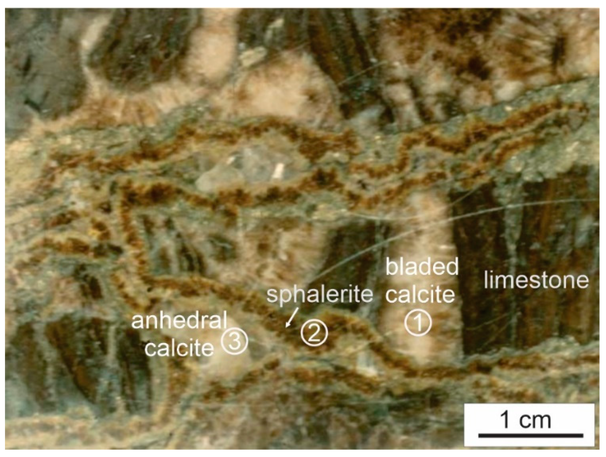
• Paragenetic study is essential for any fluid inclusion study. Conducting a fluid inclusion study without knowing the paragenetic position of the host mineral may lead to serious problems in data interpretation.
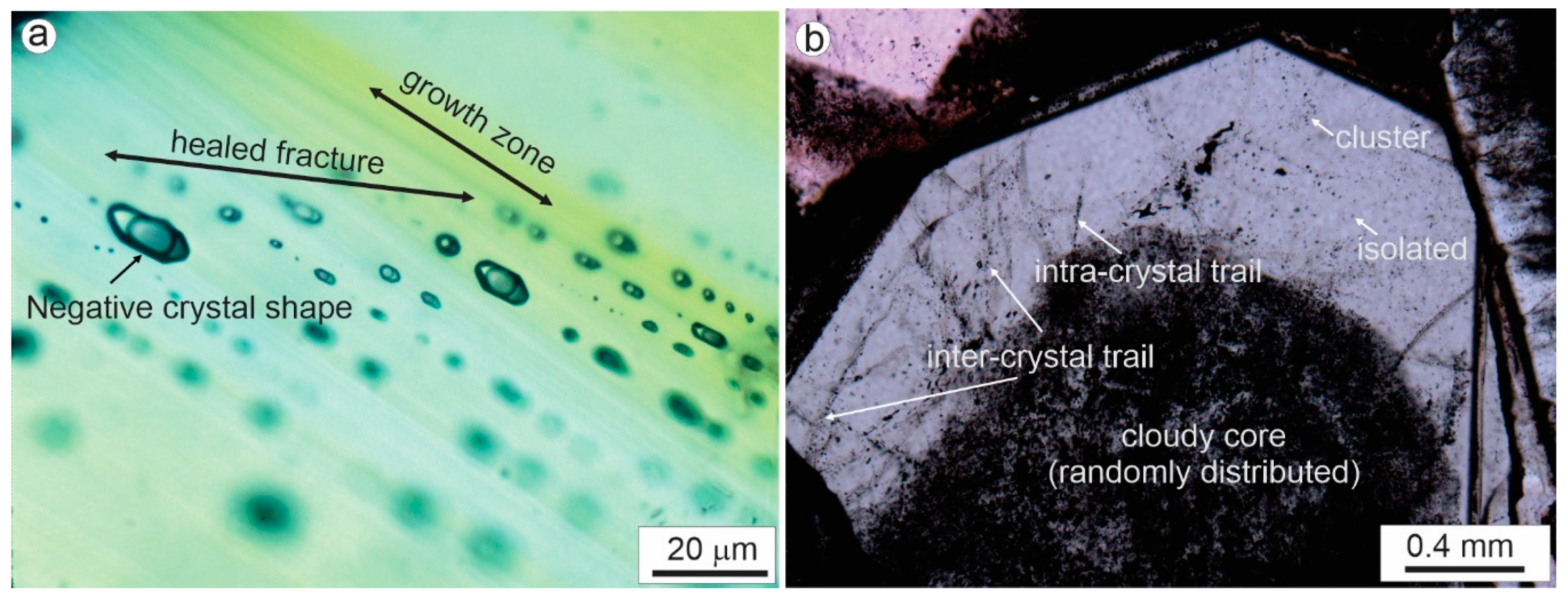
• It is often difficult to unambiguously classify fluid inclusions as primary. Assigning fluid inclusions as “primary” without describing the supporting textural evidence may create problems in the interpretation of data.
• It is important to use the ‘fluid inclusion assemblage’ (FIA) approach as much as possible to select fluid inclusions for study. Even if individual FIAs cannot be determined unambiguously, the FIA concept should be applied to constrain the validity of the microthermometric data and their interpretations.
• The first melting temperature should not be described as the “eutectic temperature”, because in many cases, fluid inclusions do not freeze completely even at the temperature of liquid nitrogen. The terms “first melting” or “apparent eutectic” are descriptive and therefore preferred.
• Liquid-only inclusions should not be excluded from study simply because they cannot yield microthermometric data. In the case of vadose-zone fluid entrapment, liquid-only inclusions are the only inclusions that can provide valid P–T information about the paleofluids. In some other low-temperature environments such as early diagenesis, liquid-only inclusions may truly record the P–T conditions of trapping, whereas biphase inclusions may have resulted from post-entrapment modification.
• Final ice-melting temperatures measured without the presence of the vapor phase cannot be used to calculate fluid salinity due to metastability.
• It is important to specify if a fluid inclusion homogenizes into the liquid or vapor phase when classifying fluid inclusions and recording their phase transition temperatures. Homogenization into liquid or vapor has very different implications for fluid density and pressure.
• The occurrence of multiple types of fluid inclusions in a mineral should not be simply described as “coexistence” of these types of inclusions even if they all appear to be “primary”. An examination of the compatibility of these types of fluid inclusions in terms of phase equilibria is required, and whether or not these different types of fluid inclusions can be all coeval should be evaluated accordingly.
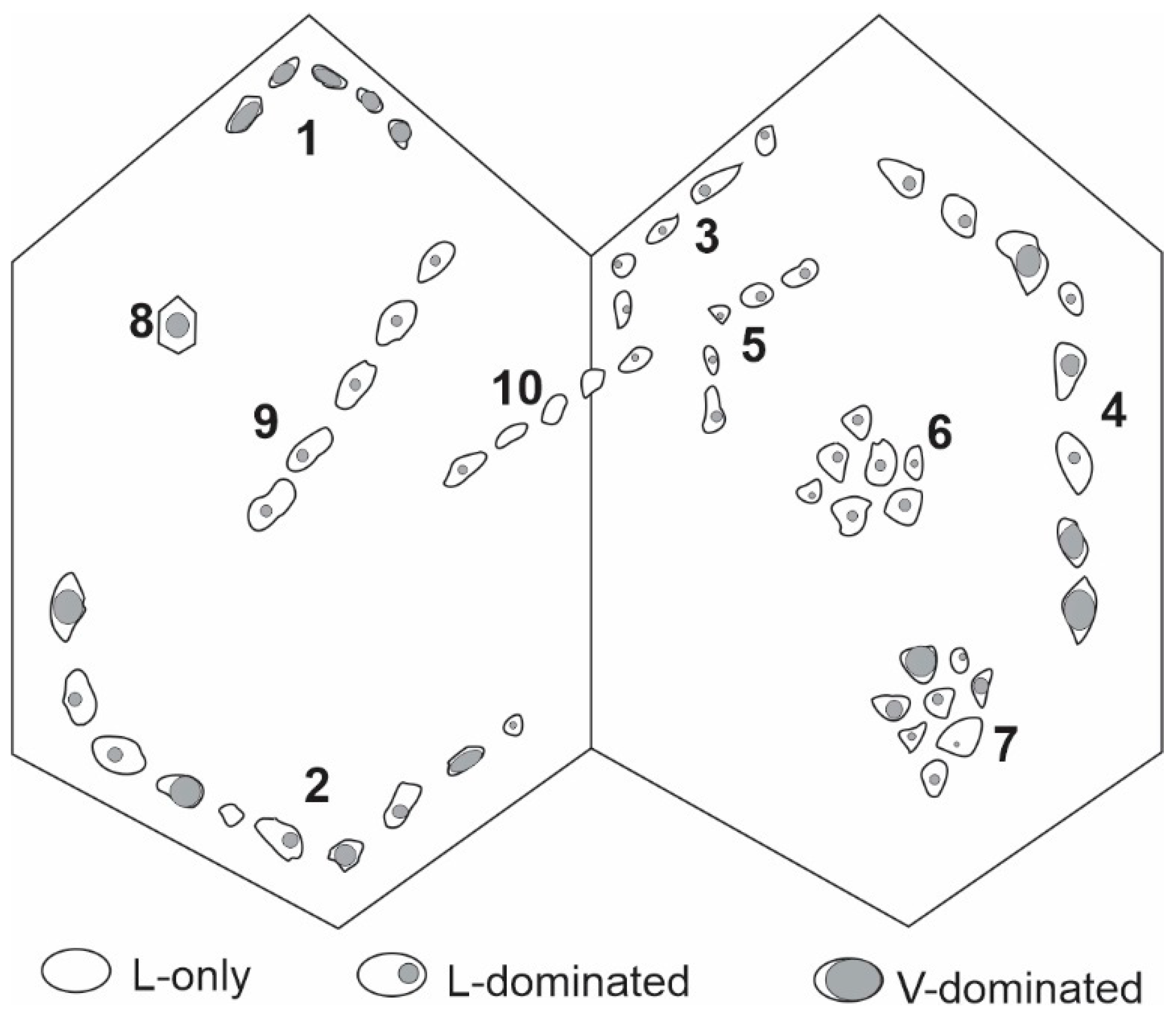
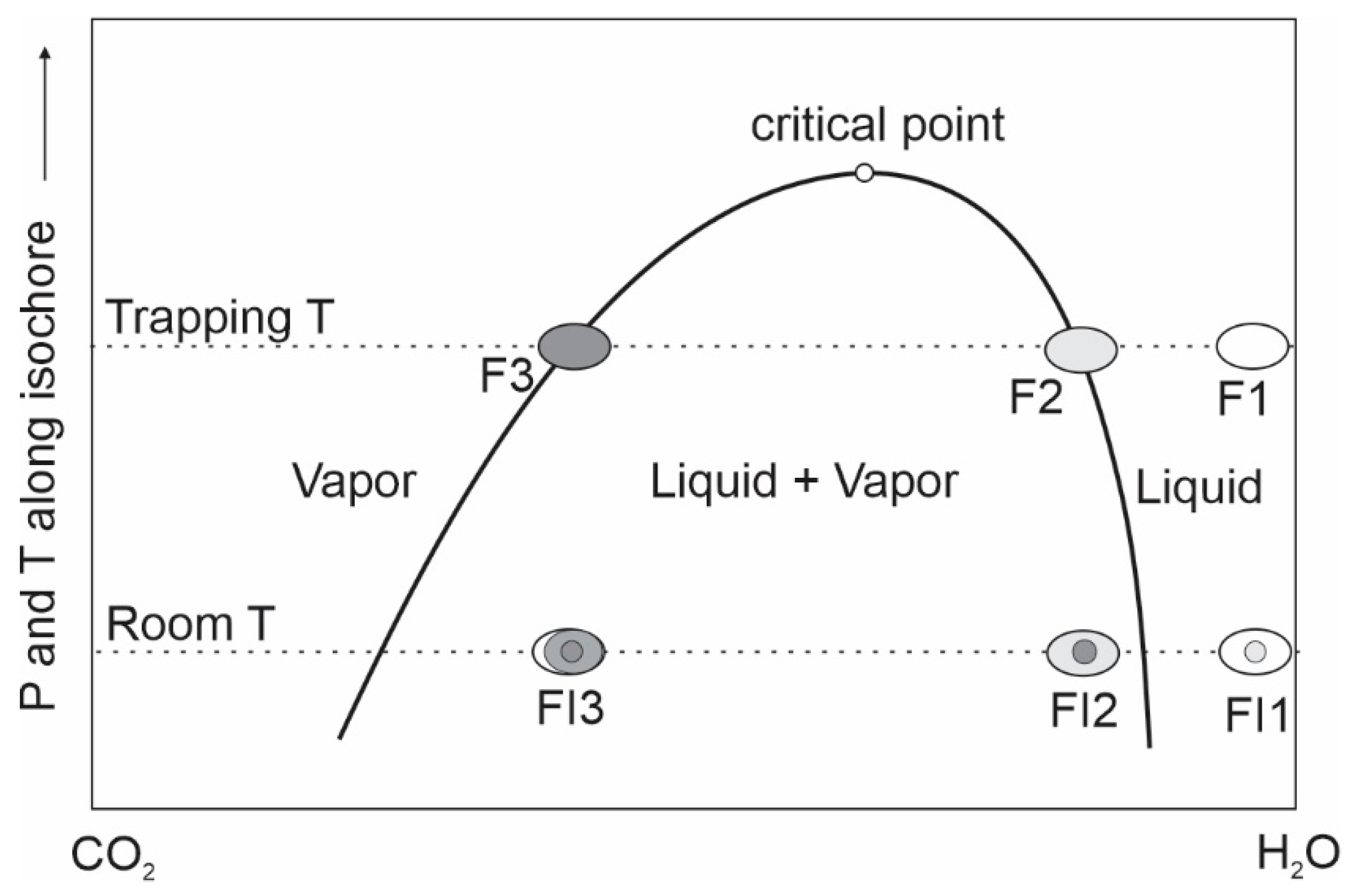
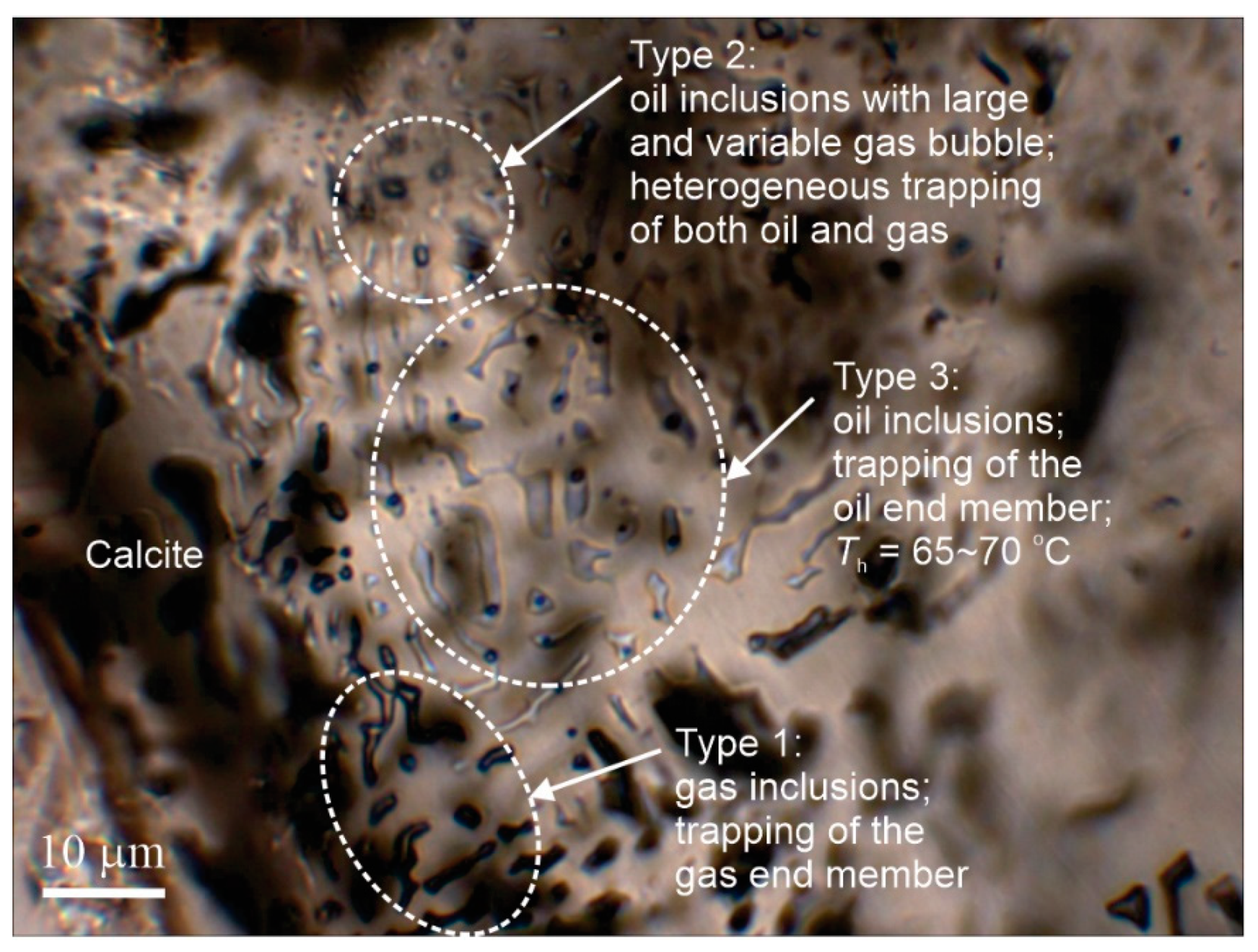
• Fluid boiling is used to describe the process of phase change from liquid to liquid + vapor for single-volatile fluid systems, whereas fluid immiscibility describes the state of coexistence of liquid and vapor for both single-volatile and multi-volatile systems. Heterogenous trapping, which produces liquid-dominated and vapor-dominated inclusions with variable homogenization temperatures, is good evidence for fluid immiscibility, but in such FIAs, only inclusions that can be proven to have trapped end-member liquid or end-member vapor yield meaningful homogenization temperatures.
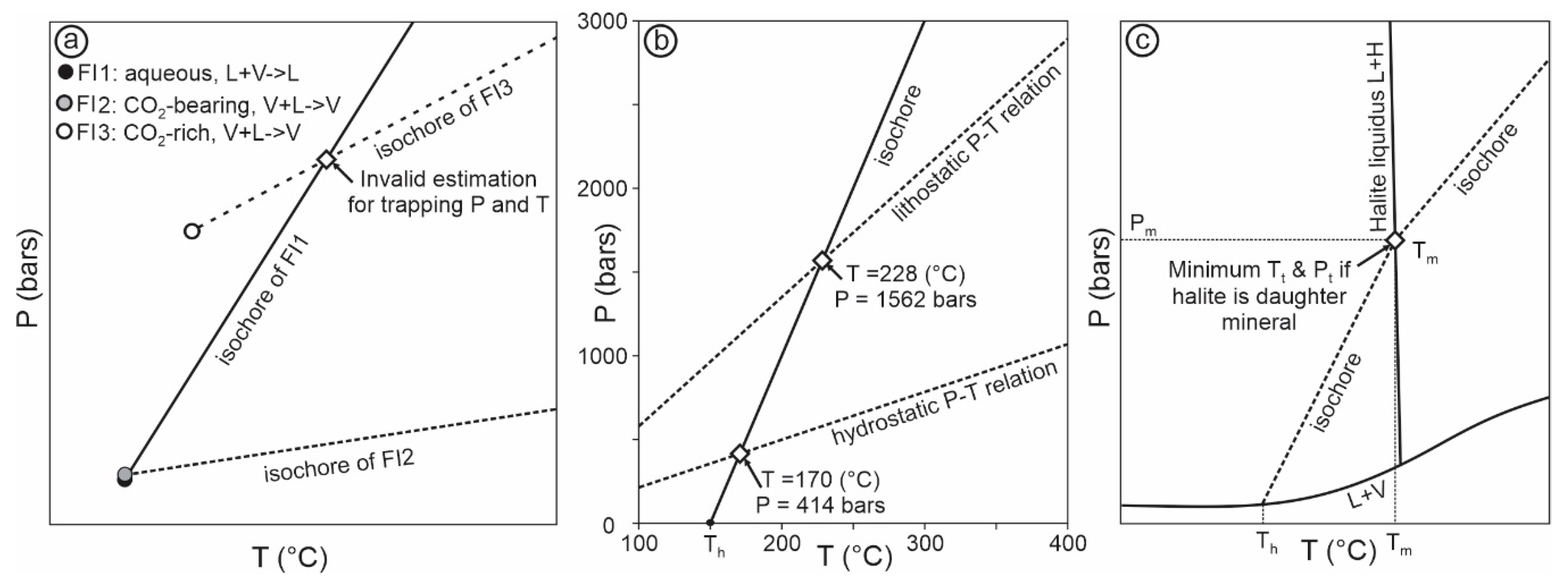
• Solid phases in fluid inclusions may be daughter minerals or accidently entrapped solids. Even if they are soluble salt crystals, they should not be automatically interpreted as daughter minerals. The best evidence for the presence of daughter minerals is if they have uniform phase proportions in all inclusions within an individual FIA (and hence they have very similar melting temperatures).
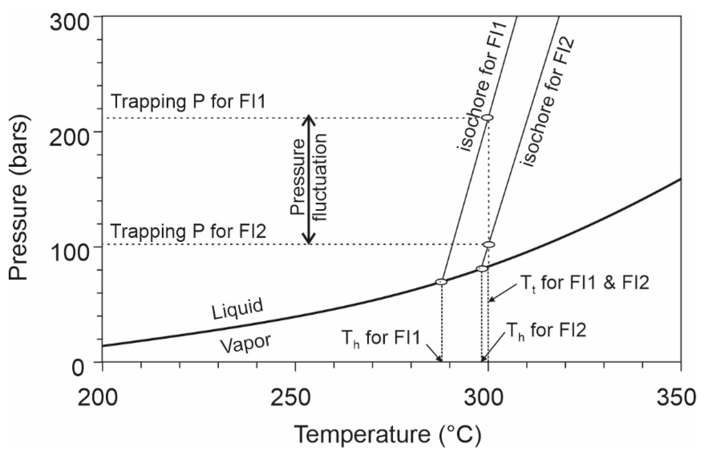
• The wide range of homogenization temperatures documented in many studies may be partly attributed to artifacts and partly to real P–T fluctuation. The common artifacts include failure to recognize different generations of fluid inclusions, heterogeneous trapping and post-entrapment modifications (e.g., necking down through a phase boundary, stretching, deformation of the host crystal). Even after the exclusion of the artifacts, the range of homogenization temperatures should not be simply considered as reflecting the variation of fluid temperature, as pressure fluctuation can also result in variation of homogenization temperatures.
• Although fluid pressure is one of the most important parameters that one may aim to estimate from fluid inclusion studies, the uncertainties of fluid pressure calculation are generally higher than assumed. The uncertainties include those inherent to the chosen equation-of-state, the sensitivity of pressure to temperature as governed by the equations, and those involved in the estimation of the trapping temperatures. It is important to know the limit of the various fluid pressure calculation methods in order to avoid overinterpretation of the meaning of the fluid pressure values.
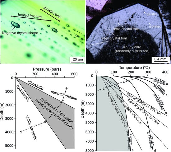
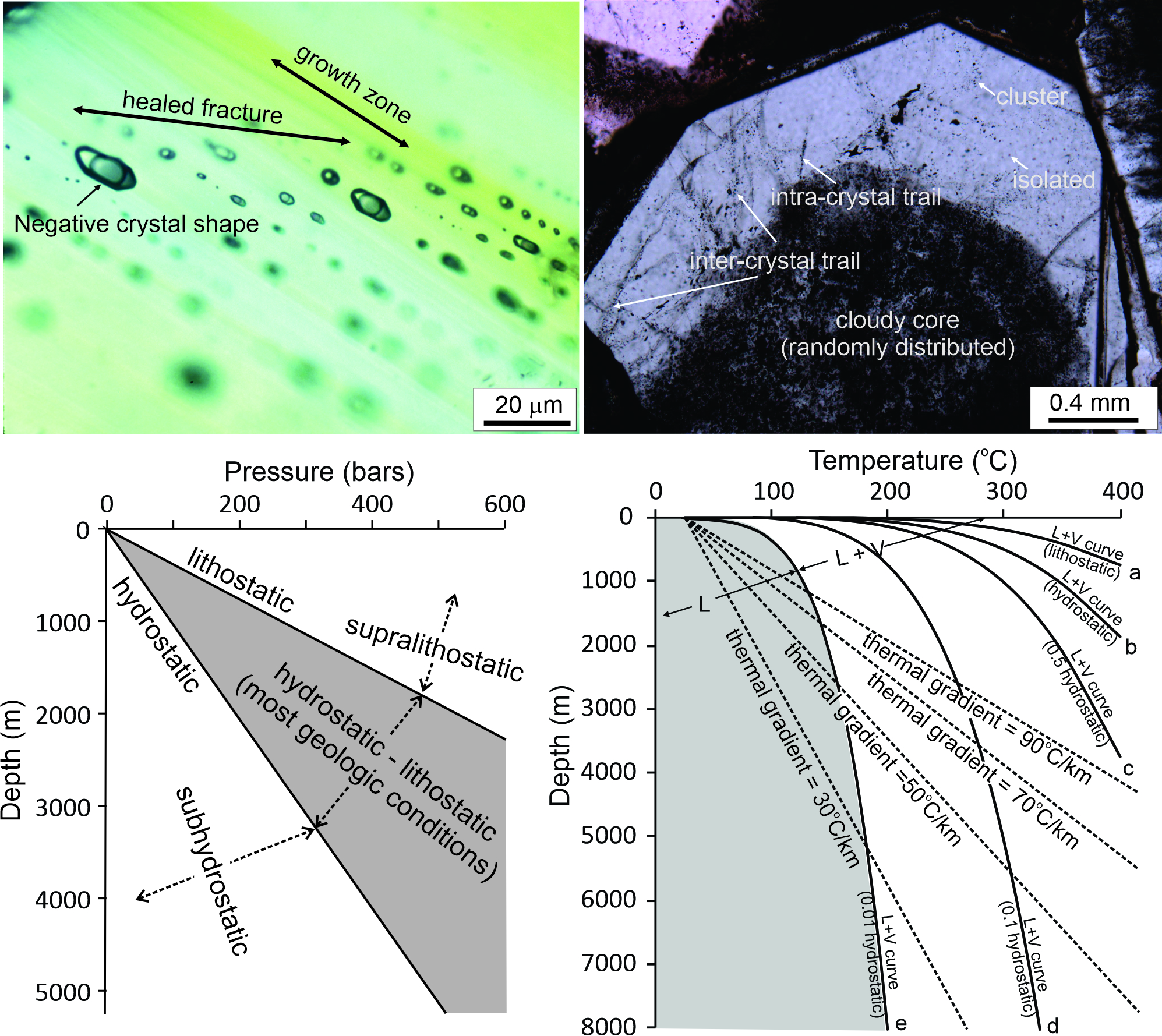
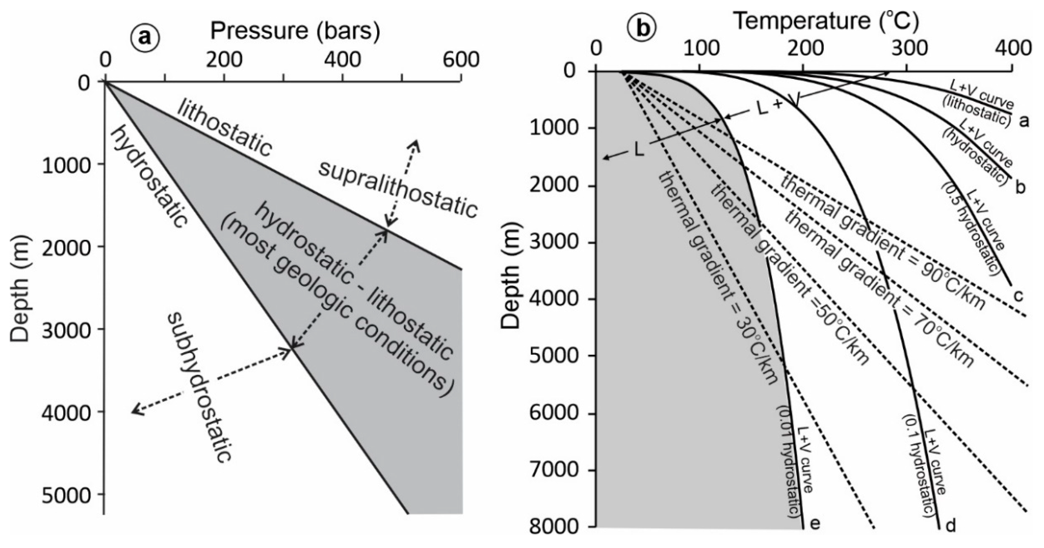
• The ultimate purpose of fluid pressure calculation is often to estimate the depth. However, it should be emphasized that even if fluid pressure has been constrained with confidence, it is not straightforward to calculate depth from fluid pressure. Much of the uncertainty comes from the difficulty in determining the fluid pressure regime, which may vary from subhydrostatic to supralithostatic.
• Bulk fluid inclusion analyses are useful methods for determining the compositions of paleofluids. However, the meaningful application of these methods requires that the sample contains a single or at least a dominant generation of fluid inclusions that are of interest. This requirement should not be neglected in sample preparation and data interpretation.
• Although raw data may not be accommodated in a publication, they should be provided in supplementary material. Detailed information about fluid inclusion occurrences and phase changes at homogenization should be described. The number of digits after the decimal point should reflect the true precision of the microthermometric data. Fluid inclusion data should not be simply treated as any geochemical data in a statistical approach. The quality of the data is more important than the quantity. The average value rather than that of each inclusion within an individual FIA should be used in diagrams in order to avoid overrepresentation (some FIA allow many more measurements than others), and the significance of the range of a parameter should not be masked by the average or peak in a diagram.
• Despite the many potential problems, fluid inclusion study remains an indispensable method for studying paleofluids. Knowing the potential problems and taking steps to avoid them or minimize their impact are critical for a successful fluid inclusion study.

References

1. Sorby, H.C. On the microscopical structure of crystals, indicating the origin of minerals and rocks. Geol. Soc. London Quart. J. 1858, 14, 453–500. [Google Scholar] [CrossRef]
2. Hollister, L.S.; Crawford, M.L. (Eds.) Fluid Inclusions-Applications in Petrology; Mineralogical Association of Canada Publications: Québec, QC, Canada, 1981; Volume 6, p. 304. [Google Scholar]
3. Roedder, E. Fluid inclusions. Geol. Soc. Am. Bull. 1984, 12, 644. [Google Scholar]
4. Shepherd, T.J.; Rankin, A.H.; Alderton, D.H.M. A Practical Guide to Fluid Inclusion Studies; Blackie: Glasgow, Scotland, UK, 1985; p. 239. [Google Scholar]
5. Anderson, T.; Frezzotti, M.-L.; Burke, E.A.J. Editorial-A tribute to Jacques Touret. Lithos 2001, 55, ix–xi. [Google Scholar] [CrossRef]
6. Samson, I.; Anderson, A.; Marshall, D. (Eds.) Fluid Inclusions. Analysis and Interpretation; Mineralogical Association of Canada Publications: Québec, QC, Canada, 2003; Volume 32, p. 374. [Google Scholar]
7. Lu, H.; Fan, H.; Ni, P.; Ou, G.; Shen, K.; Zhang, W. Fluid Inclusions; Science Press: Beijing, China, 2004; p. 487. (In Chinese) [Google Scholar]
8. Hurai, V.; Huraiová, M.; Slobodník, M.; Thomas, R. Geofluids: Developments in Microthermometry, Spectroscopy, Thermodynamics, and Stable Isotopes; Elsevier: Amsterdam, The Netherlands, 2015; p. 489. [Google Scholar]
9. Roedder, E.; Bodnar, R.J. Fluid inclusion studies of hydrothermal deposits. In Geochemistry of Hydrothermal Ore Deposits, 3rd ed.; Barnes, H.L., Ed.; John Wiley & Sons: New York, NY, USA, 1997; pp. 657–698. [Google Scholar]
10. Wilkinson, J.J. Fluid inclusions in hydrothermal ore deposits. Lithos 2001, 55, 229–272. [Google Scholar] [CrossRef]
11. Bodnar, R.J.; Lecumberri-Sanchez, P.; Moncada, D.; Steele-MacInnis, M. Fluid inclusions in hydrothermal ore deposits. In Treatise on Geochemistry, 2nd ed.; Holland, H.D., Turekian, K.K., Eds.; Elsevier: Oxford, UK, 2014; Volume 13, pp. 119–142. [Google Scholar]
12. Chi, G. Constraints from fluid inclusion studies on hydrodynamic models of mineralization. Acta. Petrol. Sin. 2015, 31, 907–917. [Google Scholar]
13. Roedder, E.; Bodnar, R.J. Geologic pressure determinations from fluid inclusion studies. An. Rev. Earth Planet Sci. 1980, 8, 263–301. [Google Scholar] [CrossRef]
14. Goldstein, R.H.; Reynolds, T.J. Systematics of Fluid Inclusions in Diagenetic Minerals. Soc. Sed. Geol. Short Course 1994, 31, 199. [Google Scholar]
15. Goldstein, R.H. Fluid inclusions in sedimentary and diagenetic systems. Lithos 2001, 55, 159–193. [Google Scholar] [CrossRef]
16. Gagnon, J.E.; Samson, I.M.; Fryer, B.J. LA-ICP-MS analysis of fluid inclusions. In Fluid Inclusions: Analysis and Interpretation; Samson, I., Anderson, A., Marshall, D., Eds.; Mineralogical Association of Canada Publications: Québec, QC, Canada, 2003; Volume 32, pp. 291–322. [Google Scholar]
17. Frezzotti, M.L.; Tecce, F.; Casagli, A. Raman spectroscopy for fluid inclusion analysis. J. Geochem. Explor. 2012, 112, 1–20. [Google Scholar] [CrossRef]
18. Van den Kerkhof, A.M.; Hein, U. Fluid inclusion petrography. Lithos 2001, 55, 27–47. [Google Scholar] [CrossRef]
19. Bodnar, R.J. Introduction to fluid inclusions. In Fluid Inclusions: Analysis and Interpretation; Samson, I., Anderson, A., Marshall, D., Eds.; Mineralogical Association of Canada Publications: Québec, QC, Canada, 2003; Volume 32, pp. 1–8. [Google Scholar]
20. Lambrecht, G.; Diamond, L.W. Morphological ripening of fluid inclusions and coupled zone-refining in quartz crystals revealed by cathodoluminescence imaging: Implications for CL-petrography, fluid inclusion analysis and trace-element geothermometry. Geochim. Cosmochim. Acta 2014, 141, 381–406. [Google Scholar] [CrossRef]
21. Diamond, L.W.; Tarantola, A. Interpretation of fluid inclusions in quartz deformed by weak ductile shearing: Reconstruction of differential stress magnitudes and pre-deformation fluid properties. Earth Planet. Sci. Lett. 2015, 417, 107–119. [Google Scholar] [CrossRef]
22. Diamond, L.W. Fluid inclusion evidence for P-V-T-X evolution of hydrothermal solution in late-Alpine gold-quartz veins at Brusson, Val d’Ayas, northwest Italian Alps. Am. J. Sci. 1990, 290, 912–958. [Google Scholar] [CrossRef]
23. Rabiei, M.; Chi, G.; Normand, C.; Davis, W.J.; Fayek, M.; Blamey, N. Hydrothermal REE (xenotime) mineralization at Maw Zone, Athabasca Basin, Canada, and its relationship with unconformity-related uranium deposits. Econ. Geol. 2017, 112, 1483–1507. [Google Scholar] [CrossRef]
24. Fall, A.; Bodnar, R.J. How precisely can the temperature of a fluid event be constrained using fluid inclusions? Econ. Geol. 2018, 113, 1817–1843. [Google Scholar] [CrossRef] [Green Version]
25. Wang, K.; Chi, G.; Bethune, K.M.; Li, Z.; Blamey, N.; Card, C.; Potter, E.G.; Liu, Y. Fluid P-T-X characteristics and evidence for boiling in the formation of the Phoenix uranium deposit (Athabasca Basin, Canada): Implications for unconformity-related uranium mineralization mechanisms. Ore Geol. Rev. 2018, 101, 122–142. [Google Scholar] [CrossRef]
26. Touret, J.L.R. Fluids in metamorphic rocks. Lithos 2001, 55, 1–25. [Google Scholar] [CrossRef]
27. Chi, G.; Lu, H. Validation and representation of fluid inclusion microthermometric data using the fluid inclusion assemblage (FIA) concept. Acta. Petrol. Sin. 2008, 9, 1945–1953. [Google Scholar]
28. Roedder, E. Changes in ore fluid with time, from fluid inclusion studies at Creede, Colorado. In Proceedings of the IAGOD 4th Symposium, Varna, Bulgaria, 19–25 September 1977; pp. 179–185. [Google Scholar]
29. Haynes, F.M. Determination of fluid inclusion compositions by sequential freezing. Econ. Geol. 1985, 80, 1436–1439. [Google Scholar] [CrossRef]
30. Diamond, L.W. Stability of CO2-clathrate-hydrate + CO2 liquid + CO2 vapour + aqueous KCl-NaCl solutions: Experimental determination and application to salinity estimates of fluid inclusions. Geochim. Cosmochim. Acta 1992, 56, 273–280. [Google Scholar] [CrossRef]
31. Steele-MacInnis, M.; Bodnar, R.J.; Naden, J. Numerical mode to determine the composition of H2O-NaCl-CaCl2 fluid inclusions based on microthermometric and microanalytical data. Geochim. Cosmochim. Acta 2011, 75, 21–40. [Google Scholar] [CrossRef] [Green Version]
32. Samson, I.M.; Walker, R.T. Cryogenic Raman spectroscopic studies in the system NaCl-CaCl2-H2O and implications for low-temperature phase behavior in aqueous fluid inclusions. Can. Mineral. 2000, 38, 35–43. [Google Scholar] [CrossRef] [Green Version]
33. Baumgartner, M.; Bakker, R.J. CaCl2-hydrate nucleation in synthetic fluid inclusions. Chem. Geol. 2009, 265, 335–344. [Google Scholar] [CrossRef]
34. Chu, H.; Chi, G.; Chou, I.-M. Freezing and melting behaviors of H2O-NaCl-CaCl2 solutions in fused silica capillaries and glass-sandwiched films: Implications for fluid inclusion studies. Geofluids 2016, 16, 518–532. [Google Scholar] [CrossRef] [Green Version]
35. Davis, D.W.; Lowenstein, T.K.; Spencer, R.J. Melting behavior of fluid inclusions in laboratory-grown halite crystals in the systems NaCl-H2O, NaCl-KCl-H2O, NaCl-MgCl2-H2O, and NaCl-CaCl2-H2O. Geochim. Cosmochim. Acta 1990, 54, 591–601. [Google Scholar] [CrossRef]
36. Diamond, L.W. Systematics of H2O inclusions. In Fluid Inclusions: Analysis and Interpretation; Samson, I., Anderson, A., Marshall, D., Eds.; Mineralogical Association of Canada Publications: Québec, QC, Canada, 2003; Volume 32, pp. 55–79. [Google Scholar]
37. Kruger, Y.; Stoller, P.; Ricka, J.; Frenz, M. Femtosecond lasers in fluid-inclusion analysis: Overcoming metastable phase states. Eur. J. Miner. 2007, 19, 693–706. [Google Scholar] [CrossRef] [Green Version]
38. Diamond, L.W. Review of the systematics of CO2–H2O fluid inclusions. Lithos 2001, 55, 69–99. [Google Scholar] [CrossRef]
39. Pichavant, M.; Ramboz, C.; Weisbrod, A. Fluid immiscibility in natural processes: Use and misuse of fluid inclusion data. I. Phase equilibria analysis-A theoretical and geometrical approach. Chem. Geol. 1982, 37, 1–27. [Google Scholar] [CrossRef]
40. Mernagh, T.P.; Leys, C.; Henley, R.W. Fluid inclusion systematics in porphyry copper deposits: The super-giant Grasberg deposit, Indonesia, as a case study. Ore Geol. Rev. 2020, 123, 103570. [Google Scholar] [CrossRef]
41. Ramboz, C.; Pichavant, M.; Weisbrod, A. Fluid immiscibility in natural processes: Use and misuse of fluid inclusion data. II. Interpretation of fluid inclusion data in terms of immiscibility. Chem. Geol. 1982, 37, 29–48. [Google Scholar] [CrossRef]
42. Belkin, H.; De Vivo, B.; Gianelli, G.; Lattanzi, P. Fluid inclusions in minerals from the geothermal fields of Tuscany, Italy. Geothermics 1985, 14, 59–72. [Google Scholar] [CrossRef]
43. Bali, E.; Aradi, L.E.; Zierenberg, R.; Diamond, L.W.; Pettke, T.; Szabó, A.; Guðfinnsson, G.H.; Friðleifsson, G.O.; Szabó, C. Geothermal energy and ore-forming potential of 600 °C mid-ocean-ridge hydrothermal fluids. Geology 2020, 48, 1221–1225. [Google Scholar] [CrossRef]
44. Mavrogenes, J.A.; Bodnar, R.J. Hydrogen movement into and out of fluid inclusions in quartz: Experimental evidence and geologic implications. Geochim. Cosmochim. Acta 1994, 58, 141–148. [Google Scholar] [CrossRef]
45. Campbell, A.R.; Lundberg, S.A.W.; Dunbar, N.W. Solid inclusions of halite in quartz: Evidence for the halite trend. Chem. Geol. 2001, 173, 179–191. [Google Scholar] [CrossRef] [Green Version]
46. Becker, S.P.; Fall, A.; Bodnar, R.J. Synthetic fluid inclusions. XVII. PVTX properties of high salinity H2O-NaCl solutions (>30 wt. % NaCl): Application to fluid inclusions that homogenize by halite disappearance from porphyry copper and other hydrothermal ore deposits. Econ. Geol. 2008, 103, 539–554. [Google Scholar] [CrossRef]
47. Lecumberri-Sanchez, P.; Steele MacInnis, M.; Bodnar, R.J. A numerical model to estimate trapping conditions of fluid inclusions that homogenize by halite disappearance. Geochim. Cosmochim. Acta 2012, 92, 14–22. [Google Scholar] [CrossRef]
48. Bakker, R.J. Package FLUIDS 1. Computer programs for analysis of fluid inclusion data and for modelling bulk fluid properties. Chem. Geol. 2003, 194, 3–23. [Google Scholar] [CrossRef]
49. Bodnar, R.J. Philosophy of fluid inclusion analysis. In Minerals, Methods and Applications; De Vivo, B., Frezzotti, M.L., Eds.; Virginia Tech: Blacksburg, VA, USA, 1994; pp. 1–6. [Google Scholar]
50. Steele-MacInnis, M.; Lecumberri-Sanchez, P.; Bodnar, R.J. Hokieflincs_H2O-NACL: A Microsoft Excel spreadsheet for interpreting microthermometric data from fluid inclusions based on the PVTX properties of H2O–NaCl. Comput. Geosci. 2012, 49, 334–337. [Google Scholar] [CrossRef]
51. Sibson, R.H.; Robert, F.; Poulsen, K.H. High angle reverse faults, fluid pressure cycling, and mesothermal gold-quartz deposits. Geology 1988, 16, 551–555. [Google Scholar] [CrossRef]
52. Chi, G.; Guha, J.; Lu, H.-Z. Separation mechanism in the formation of proximal and distal tin-polymetallic deposits, Xinlu ore field, southern China-Evidence from fluid inclusion data. Econ. Geol. 1993, 88, 916–933. [Google Scholar] [CrossRef]
53. Richter, L.; Diamond, L.W.; Atanasova, P.; Banks, D.A.; Gutzmer, J. Hydrothermal formation of heavy rare earth element (HREE)-xenotime deposits at 100oC in a sedimentary basin. Geology 2018, 46, 263–266. [Google Scholar] [CrossRef] [Green Version]
54. Sibson, R.H.; Moore, J.M.M.; Rankin, A.H. Seismic pumping—A hydrothermal fluid transport mechanism. J. Geol. Soc. 1975, 131, 653–659. [Google Scholar] [CrossRef]
55. Gleeson, S.A. Bulk analysis of electrolytes in fluid inclusions. In Fluid Inclusions: Analysis and Interpretation; Samson, I., Anderson, A., Marshall, D., Eds.; Mineralogical Association of Canada Publications: Québec, QC, Canada, 2003; Volume 32, pp. 233–246. [Google Scholar]
56. Blamey, N.J.F. Compositional and evolution of crustal, geothermal, and hydrothermal fluids interpreted using quantitative fluid inclusion gas analysis. J. Geochem. Explor. 2012, 116–117, 17–27. [Google Scholar] [CrossRef]
Figure 1. A hand sample showing three hydrothermal mineral phases representing different stages of the fluid system: pre-mineralization bladed calcite ①, syn-mineralization sphalerite ②, and post-mineralization anhedral calcite ③. The sample is from the Jubilee carbonate-hosted Zn-Pb deposit, Nova Scotia, Canada.
Minerals 11 00007 g001
Figure 2. (a) Secondary fluid inclusions with negative crystal shape in a healed fracture (shown by distribution of fluid inclusions on the same focus plane) crosscutting growth zones (shown by color variation) in a cassiterite crystal; the sample is from the Dongjia’ao Sn deposit, Guangxi, China. (b) Various modes of occurrences of fluid inclusions in a quartz crystal, including randomly (and densely) distributed inclusions in the cloudy core overgrown by a relatively clean rim, with fluid inclusions occurring in clusters, intra-crystal trails, inter-crystal trails and as isolated ones in the rim; note the fluid inclusions are not simply labeled as primary, pseudosecondary or secondary, as discussed in the text; the sample is from the Beaverlodge uranium district, Saskatchewan, Canada.
Minerals 11 00007 g002
Figure 3. A schematic example of various modes of occurrence of fluid inclusions with an emphasis on fluid inclusion assemblages (FIAs). See text for detailed discussion.
Minerals 11 00007 g003
Figure 4. A schematic phase diagram for the H2O–CO2 system (modified from [38]) illustrating that a maximum of two fluid phases can coexist at the trapping condition, representing the liquid (F2) and vapor (F3) phases that confine the liquid + vapor immiscibility field. An additional liquid phase (F1) cannot coexist with F2 because they are in the one-phase (liquid) field.
Minerals 11 00007 g004
Figure 5. A fluid inclusion assemblage (FIA) in a healed fracture in calcite consisting of three types of fluid inclusions suggesting oil–gas immiscibility. The vapor-dominated inclusions and liquid-dominated inclusions represent trapping of the vapor (gas) and liquid (oil) end-members respectively, whereas the inclusions with large and variable vapor/liquid ratios result from heterogeneous trapping of both oil and gas phases. The sample is from the July Lake area, British Columbia, Canada.
Minerals 11 00007 g005
Figure 6. P–T phase diagram for a H2O–NaCl system with a salinity of 10 wt% showing the liquid–vapor boundary and isochores of two fluid inclusions entrapped at different P–T conditions, illustrating how fluctuation of fluid pressure between lithostatic and hydrostatic values may result in a variation of Th values of fluid inclusions without changing the trapping temperature. Isochores and liquid–vapor phase boundaries were calculated with the program of Steele-MacInnis et al. (2012) [50]. See text for discussion.
Minerals 11 00007 g006
Figure 7. (a) Schematic diagram showing isochores of an aqueous inclusion (homogenized to liquid; FI1), a CO2-bearing inclusion (homogenized to vapor; FI2), and a CO2-rich inclusion (homogenized to vapor; FI3). Note if FI1 and FI2 are interpreted to represent immiscible fluid phases entrapped at the same time, then their homogenization temperature and pressure represent the Tt and Pt; FI1 and FI3 cannot be entrapped at the same time unless they can be proven to be physically separated, and their intersection cannot be used to indicating the Tt and Pt. (b) Isochore for a fluid inclusion with a Th of 150 °C and salinity of 10 wt% NaCl (calculated with the program of Steele-MacInnis et al., 2012 [50]) and its intersections with P–T relations for a geothermal gradient of 35 °C/km for lithostatic and hydrostatic pressure regimes; note the large difference in estimated Tt and Pt for the two different pressure regimes. (c) Schematic diagram showing part of the phase relationships of the H2O–NaCl system including the liquid–vapor curve and the halite liquidus and the isochore of a fluid inclusion, whose halite dissolution temperature (Tm) is higher than vapor disappearance temperature (Th) (modified from [46]); note that if the halite cannot be proven to be daughter mineral, then the Ts and corresponding pressure (Pm) do not represent the minimum Tt and Pt.
Minerals 11 00007 g007
Figure 8. (a) Relationships between fluid pressure and depth for different pressure regimes (lithostatic, hydrostatic, subhydrostatic, supralithostatic). (b) Liquid–vapor curve in a depth–temperature space for a fluid with 20 wt% NaCl (computed with the program from Steele-McInnis et al. 2012 [50]) at different fluid pressure regimes (lithostatic, hydrostatic, 0.5 hydrostatic, 0.1 hydrostatic, and 0.01 hydrostatic). See text for discussion.
Minerals 11 00007 g008
Publisher’s Note: MDPI stays neutral with regard to jurisdictional claims in published maps and institutional affiliations.