An LSTM Approach for SAG Mill Operational Relative-Hardness Prediction

Abstract

Ore hardness plays a critical role in comminution circuits. Ore hardness is usually characterized at sample support in order to populate geometallurgical block models. However, the required attributes are not always available and suffer for lack of temporal resolution. We propose an operational relative-hardness definition and the use of real-time operational data to train a Long Short-Term Memory, a deep neural network architecture, to forecast the upcoming operational relative-hardness. We applied the proposed methodology on two SAG mill datasets, of one year period each. Results show accuracies above 80% on both SAG mills at a short upcoming period of times and around 1% of misclassifications between soft and hard characterization. The proposed application can be extended to any crushing and grinding equipment to forecast categorical attributes that are relevant to downstream processes.

1. Introduction

In mining operations, the primary energy consumer is the comminution system, responsible for more than half of the entire mine consumption [1]. From all pieces of equipment that integrate the comminution circuit, the semi-autogenous grinding mill (SAG) is perhaps the most important in the system. With an aspect ratio of 2:1 (diameter to length), these mills combine impact, attrition and abrasion to reduce the ore size. SAG mills are located at the beginning of the comminution circuits, after a primary crushing stage. Although there are small SAG mills, their size usually ranges from 9.8 × 4.3 to 12.8 × 7.6 m, with a nominal energy demand of 8.2 and 26 MW, respectively [2], which make SAG mills the most relevant energy consumer within the concentrator. Modelling their consumption behaviour supports the operational control and energy demand-side management [3].

Most theoretical and empirical models [4,5,6] demand input feed characteristics, such as hardness, size distribution and inflow rate, SAG characteristics, such as sizing and product size distribution, and operational variables such as bearing pressure, water addition and grinding charge level. Although they are suitable to provide adequate design guidelines, they lack accurate in-situ inference since most assume steady-state and isolation from up and downstream processes. In response, model predictive control, SAG MPC [7], combines those methods with real-time operational information. However, expert knowledge is required to model the SAG mill dynamics properly.

From a geometallurgical perspective, the integration of new predictive methods that account for space and time relationships over real-time attributes has been defined as a fundamental challenge [8,9] in mining operations, particularly in an integrated system such as comminution. In response, data-driven approaches have been proposed ranging from support vector machines [10] and gene expression programming [11] to hybrid models that combine genetic algorithms and neural networks [12] and recurrent neural networks [13]. As data-driven methods are sensitive to the context (available information) and representation (information workflow), the authors have studied the use of several machine learning and deep learning methods in modelling the SAG energy consumption behaviour based only on operational variables [14].

The energy consumed by a SAG mill is related to several factors such as expert operator decisions, charge volume, charge specific gravity and the hardness of the feed material. Knowing the output hardness material becomes relevant for the downstream stage in the primary grinding circuit. Ore hardness can be characterized at sample support by combining the logged geological properties and the result of standardized comminution tests. They can be used to predict the hardness of each block sent to the process. However, these attributes are not always available. In response, a qualitative characterization of the ore hardness processed at time t, relative to the operational hardness of the ore processed at time $t+1$ can be done using only operational variables rather than a set of mineralogical characterizations. This qualitative characterization is referred and here used as operational relative-hardness (ORH).

We take advantage of previous works [14] by knowing that the Long Short-Term Memory (LSTM) [15] outperforms other machine learning and deep learning techniques on inferring the SAG mill energy consumption. Therefore, Section 2 presents the ORH and LSTM models, Section 3 establishes the SAG mill experimental framework, the results of which are presented in Section 4, and conclusions are drawn in Section 5.

2. Model

2.1. Operational Relative-Hardness Criteria

From the several operational parameters that can be captured and associated to SAG mill operations, we consider the energy consumption (EC) and feed tonnage (FT) to build our operational relative-hardness criteria.

{EC,FT${\}}_t$ is collected over a period of time T using a $\Delta t$ discretization. By considering the one-step forward time difference of energy consumption ($\Delta$EC${}_t=$EC${}_{t+1}-$EC${}_t$) and feed tonnage ($\Delta$ FT${}_t$ = FT${}_{t+1}-$FT${}_t$), a qualitative assessment of the operational relative-hardness can be done. For instance, if the energy consumption is increasing and the feed tonnage is constant, it can be interpreted as an increase in ore hardness relative to the previous period. Similarly, if the feed tonnage is constant and the energy decreases, a decrease in ore hardness relative to the previous period can be assumed. Particularly, when both $\Delta$EC${}_t$ and $\Delta$FT${}_t$ show the same behaviour, the SAG can be either processing ore with medium operational relative-hardness or being filled up or emptied. To avoid misclassification in this last case, the operational relative-hardness is labelled as undefined.

Table 1. Operational relative-hardness criteria based on one time-step difference of energy consumption and feed tonnage.

Energy Consumption	Feed Tonnage	Operational Relative-Hardness
Constant	Decreasing	Hard
Increasing	Constant	Hard
Increasing	Decreasing	Hard
Decreasing	Decreasing	Undefined
Increasing	Increasing	Undefined
Constant	Constant	Undefined
Constant	Increasing	Soft
Decreasing	Constant	Soft
Decreasing	Increasing	Soft

summarizes the nine combinations of states and the associated operational relative-hardness.

The qualitative labelling of $\Delta$EC${}_t$ and $\Delta$FT${}_t$ as increasing, constant or decreasing can be established based on their global distribution over the period T as:

$$\Delta {\mathrm{EC}}_t=\left\{\begin{array}{cc}\mathrm{Increasing}\hfill & \mathrm{if}\Delta E{C}_t>\lambda ·{\sigma }_{\Delta EC}\hfill \\ \mathrm{Constant}\hfill & \mathrm{if}|\Delta E{C}_t|\le \lambda ·{\sigma }_{\Delta EC}\hfill \\ \mathrm{Decreasing}\hfill & \mathrm{if}\Delta E{C}_t<-\lambda ·{\sigma }_{\Delta EC}\hfill \end{array}\right.\Delta F{T}_t=\left\{\begin{array}{cc}\mathrm{Increasing}\hfill & \mathrm{if}\Delta F{T}_t>\lambda ·{\sigma }_{\Delta FT}\hfill \\ \mathrm{Constant}\hfill & \mathrm{if}|\Delta F{T}_t|\le \lambda ·{\sigma }_{\Delta FT}\hfill \\ \mathrm{Decreasing}\hfill & \mathrm{if}\Delta F{T}_t<-\lambda ·{\sigma }_{\Delta FT}\hfill \end{array}\right.$$

(1)

where ${\sigma }_{\Delta EC}$ and ${\sigma }_{\Delta FT}$ represent the standard deviations over the period T of $EC$ and $FT$, respectively, and $\lambda$ is a scalar value that modulates the labelling distribution. Note that (i) a $\lambda$ value above 1.5 would make the entire definition meaningless since most values would remain as constant, and (ii) the $\lambda$ value definition is an external model parameter and can be guided either subjectively or via statistical meaning.

2.2. Long Short-Term Memory

The Long Short-Term Memory (LSTM) [15] neural network architecture belongs to the family of recurrent neural networks in Deep Learning [16]. They are suitable to capture short and long term relationships in temporal datasets. Internally, LSTM applies several combinations of affine transformations, element-wise multiplications and non-linear transfer functions, for which the building blocks are:

• ${\mathbf{x}}_t$: input vector at time t. Dimension $(m,1)$.
• ${\mathbf{W}}_f,{\mathbf{W}}_i$, ${\mathbf{W}}_c$, ${\mathbf{W}}_o$: weight matrices for $x_t$. Dimensions $(n_H,m)$.
• $h_t$: hidden state at time t. Dimension $(m,1)$.
• ${\mathbf{U}}_f,{\mathbf{U}}_i$, ${\mathbf{U}}_c$, ${\mathbf{U}}_o$: weight matrices for $h_{t-1}$. Dimensions $(n_H,m)$.
• ${\mathbf{b}}_f,{\mathbf{b}}_i$, ${\mathbf{b}}_c$, ${\mathbf{b}}_o$: bias vectors. Dimensions $(n_H,1)$.
• $\mathbf{V}$: weight matrix for $h_t$ as output. Dimension $(K,m)$.
• $\mathbf{c}$: bias vector for output. Dimension $(K,1)$.

where m is the number of variables as input, K is the number of output variables, and $n_H$ is the number of hidden units. Let $\tau \in \mathbb{N}$ be a temporal window. At each time $t\in \{1,\dots ,\tau \}$, the LSTM receives the input ${\mathbf{x}}_t$, the previous hidden state $h_{t-1}$ and previous memory cell $c_{t-1}$. The forget gate $f_t=\sigma \left({\mathbf{W}}_f{\mathbf{x}}_t+{\mathbf{U}}_f{h}_{t-1}+{\mathbf{b}}_f\right)$ is the permissive barrier of the information carried by ${\mathbf{x}}_t$. The input gate $i_t=\sigma \left({\mathbf{W}}_i{\mathbf{x}}_t+{\mathbf{U}}_i{h}_{t-1}+{\mathbf{b}}_i\right)$ decides the relevance of the information carried by ${\mathbf{x}}_t$. Note that both $f_t$ and $i_t$ use sigmoid $\sigma \left(x\right)={(1+e^{-x})}^{-1}$ as the activation function over a linear combination of ${\mathbf{x}}_t$ and $h_{t-1}$.

By passing the combination of ${\mathbf{x}}_t$ and $h_{t-1}$ through a Tanh function, a candidate memory cell ${\tilde{c}}_t=Tanh\left({\mathbf{W}}_c{\mathbf{x}}_t+{\mathbf{U}}_c{h}_{t-1}+{\mathbf{b}}_c\right)$ is computed. The final memory cell $c_t=f_t\odot c_{t-1}+i_t\odot {\tilde{c}}_t$ is computed as a sum of (i) what to forget from the past memory cell as an element-wise multiplication (⊙) between $f_t$ and $c_{t-1}$, and (ii) what to learn from the candidate memory cell as an element-wise multiplication (⊙) between $i_t$ and ${\tilde{c}}_t$.

Similar to $i_t$ and $f_t$ the output gate $o_t=\sigma \left({\mathbf{W}}_o{\mathbf{x}}_t+{\mathbf{U}}_o{h}_{t-1}+{\mathbf{b}}_o\right)$ passes through a sigmoid function a linear combination between ${\mathbf{x}}_t$ and $h_{t-1}$. It controls the information passing from the current memory cell $c_t$ to the final hidden state $h_t=Tanh\left(c_t\right)\odot o_t$ as an element-wise multiplication between $o_t$ and $Tanh\left(c_t\right)$. At the final step $\tau$, the output is computed as $y_{\tau }=\left(\mathbf{V}{h}_{\tau }+\mathbf{c}\right)$. When dealing with more than one categorical prediction ($K>1$), as in the present work for ORH forecasting, a softmax function is applied over ${\mathbf{y}}_{\tau }$ to obtain the normalized probability distribution, and the category k has a probability of $\widehat{p}\left(k\right)={\displaystyle \frac{exp\left(y_{\tau ,k}\right)}{{\sum }_{c=1}^{K}exp\left(y_{\tau ,c}\right)}}$.

An illustrative scheme of the internal connection at time step t inside an LSTM is shown in Figure 1 (left). The ORH prediction has three categories (hard, soft and undefined) and the probability is computed at the last unit, at time step $\tau$, as shown in the unrolled LSTM in Figure 1 (right).

3. Experiment

3.1. Dataset

We used two datasets containing operational data for two independent SAG mills every half hour over a total time of 340 and 331 days, respectively. Each one of the SAG mills receives fresh feed and is connected in an open circuit configuration (SABC-B) where the pebble crusher product is sent to ball mills. At each time t, the dataset contains Feed tonnage (FT) (ton/h), Energy consumption (EC) (kWh), Bearing pressure (BPr) (psi) and Spindle speed (SSp) (rpm). They are split into two main subsets (a validation dataset is not considered since the optimum LSTM architecture to train is drawn from previous work [14]): training and testing (

Table 2. Summary statistics over training testing dataset on semi-autogenous grinding mill (SAG) mills.

SAG Mill 1	Training|Testing Dataset
Variable	Min		Mean		Max		St Dev		Count
Feed Tonnage (ton/h)	0	0	911	884	2111	1953	497	480	8170	8170
Energy Consumption (kWh)	0	0	9927	8920	12,248	10,809	1245	959	8170	8170
Bearing Pressure (psi)	0	0	12.7	11.9	13.7	13.7	2.2	2.2	8170	8170
Spindle Speed (rpm)	0	0	9.2	9.1	10.3	10.7	0.7	0.7	8170	8170
SAG Mill 2	Training|Testing Dataset
Variable	Min		Mean		Max		St Dev		Count
Feed Tonnage (ton/h)	0	0	2077	2073	3477	3452	1136	1134	7953	7952
Energy Consumption (kWh)	0	0	16,709	17,445	19,688	19,533	1504	1462	7953	7952
Bearing Pressure (psi)	0	0	13.8	14.8	18.3	18.3	3.5	3.8	7953	7952
Spindle Speed (rpm)	0	0	9.1	8.9	10.0	9.9	0.6	0.6	7953	7952

). This is an arbitrary division, and we seek to have a proportion of ∼50/50, respectively.

As it can be seen in Table 2, the predictive methods are trained with the first 50% and tested with the upcoming 50%, without being fed with the previous 50% of historical data.

Note that the comminution properties of the ore, such as $a\times b$ or BWi, are not included in the datasets; therefore, the relationship between forecasted ORH and comminution properties is not explored in this work. The results herein presented, however, serve as a basis to examine such a relationship if those properties were known.

3.2. Assumptions

SAG mills are fundamental pieces in comminution circuits. As no information regarding downstream/upstream processes is available, recognizing bottlenecks in the dataset becomes subjective. We assume that SAG mills will potentially show changes from steady-state to under capacity and vice versa along with the dataset. Thus, stationarity of all operational variable distributions is assumed throughout this work, including the ore grindability. It means that the entire dataset belongs to a known and planned combination of ore characteristics (geometallurgical units). By doing so, we limit the applicability of the present models beyond the temporal dataset without a proper training process.

As explained in the problem statement section, we make use of the temporal average over energy consumption and feed tonnage as input for operational hardness prediction. Thus, we assume an additivity property over those variables as their units are kWh and ton/h, respectively, over constant temporal discretization so averaging adjacent data points is mathematically consistent.

In the operation from which the datasets were obtained, the SAG mill liners are replaced every 5–7 months. Since the datasets cover almost a year, we can ensure that the liners were replaced in each SAG mill at least once during the tested period, which may alter the relationship between energy consumption and other operational variables, inducing a discontinuity in the temporal plots. However, since in this work the temporal window for ORH evaluation is eight hours, the local discontinuity associated with liners replacement is not expected to affect the forecast at that time frame. The ORH is related to what was happening in the corresponding mill within the last few hours, and not to the mill behaviour prior to the last replacement of liners.

3.3. Problem Statement

The aim is to forecast the operational relative-hardness. To do so, we need to label the datasets with the associated ORH category at data point. We know from Equation (1) that the ORH labelling process requires as input (i) the one-step forward differences on energy consumption ($\Delta E{C}_t$) and feed tonnage ($\Delta F{T}_t$), and (ii) a lambda ($\lambda$) value. In addition, we are interested in forecasting the ORH at different time supports.

Since the information is collected every 30 min, the upcoming energy consumption EC${}_{t+1}$ and feed tonnage FT${}_{t+1}$ at 0.5 h support are denoted simply as EC${}_{t+1}$ and FT${}_{t+1}$ in reference to EC${}_{t+1}^{\left(0.5\mathrm{h}\right)}$ and FT${}_{t+1}^{\left(0.5\mathrm{h}\right)}$, respectively. An upcoming EC and FT at 1 h support, EC${}_{t+1}^{\left(1\mathrm{h}\right)}$ and FT${}_{t+1}^{\left(1\mathrm{h}\right)}$, are computed by averaging the next two energy consumption, EC${}_{t+1}$ and EC${}_{t+2}$, and the two feed tonnage, FT${}_{t+1}$ and FT${}_{t+2}$. Similarly, by averaging the upcoming ECs and FTs, different supports can be computed. Let $\mathbf{s}$ be the time support in hours, which represents the average over a temporal interval of a given duration, then EC${}_{t+1}^{\left(\mathbf{s}h\right)}$ and FT${}_{t+1}^{\left(\mathbf{s}h\right)}$ are calculated as:

$${\mathrm{EC}}_{t+1}^{\left(\mathbf{s}h\right)}={\displaystyle \frac{{\mathrm{EC}}_{t+1}+\dots +{\mathrm{EC}}_{t+2\mathbf{s}}}{2\mathbf{s}}}{\mathrm{FT}}_{t+1}^{\left(\mathbf{s}h\right)}={\displaystyle \frac{{\mathrm{FT}}_{t+1}+\dots +{\mathrm{FT}}_{t+2\mathbf{s}}}{2\mathbf{s}}}$$

(2)

In this experiment, three different supports ($\mathbf{s}h$) are considered: 0.5, 2 and 8 h.

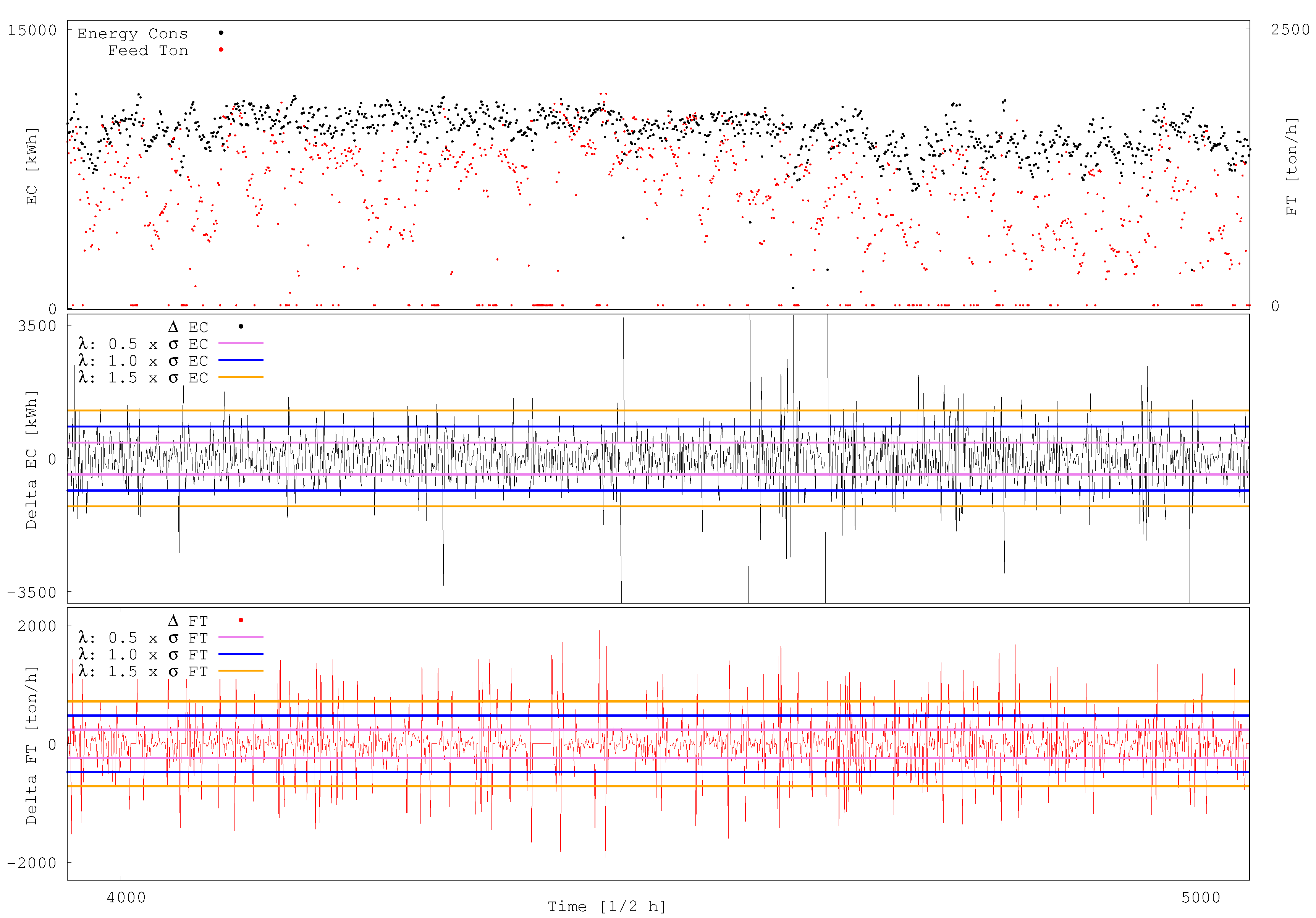
Figure 2 illustrates the ORH criteria using a half-hour time support on SAG mill 1 dataset. From the daily graph of EC${}_t^{\left(\mathbf{0}.\mathbf{5}\mathrm{h}\right)}$ and FT${}_t^{\left(\mathbf{0}.\mathbf{5}\mathrm{h}\right)}$ at the top, the graph of $\Delta$EC${}_t^{\left(\mathbf{0}.\mathbf{5}\mathrm{h}\right)}$ and $\Delta$FT${}_t^{\left(\mathbf{0}.\mathbf{5}\mathrm{h}\right)}$ are extracted and presented at the centre and bottom, respectively. Three different bands, corresponding to $\lambda$: 0.5, 1.0 and 1.5, are shown. The values that are above the band are considered as increasing, the ones below it are considered as decreasing and inside as undefined (relatively constant). The corresponding categories for EC and FT are used to define the operational relative-hardness (as in Table 1). It can be seen that, when $\lambda$ increases, the proportions of hard and soft instances decrease. 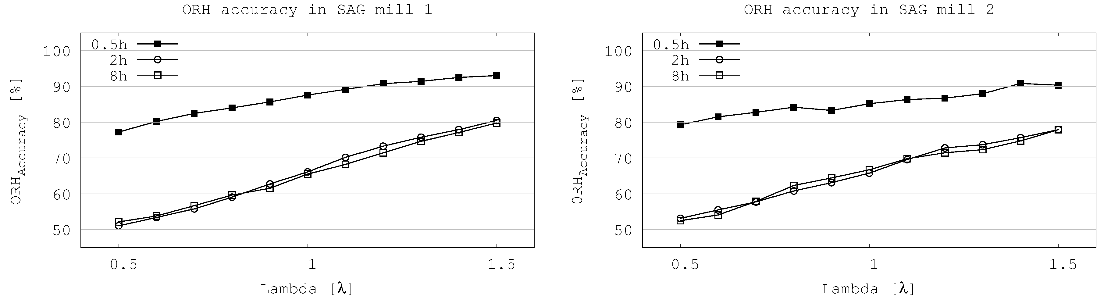Since $\lambda$ is an arbitrary parameter, a sensitivity analysis is performed in the range $[0.5,1.5]$ to capture its influence on the resulting LSTM accuracy to suitably learn to predict the ORH at the different time supports.

At each time t the input variables considered to predict ORH${}_{t+1}^{\left(\mathbf{s}h\right)}$ are FT${}_t$, BPr${}_t$ and SSp${}_t$. To account for trends, and since FT and SSp are operational decisions, the differences FT${}_{t+1}-$FT${}_t$ and SSp${}_{t+1}-$SSp${}_t$ are also considered as inputs. Therefore, the dataset of predictors and output $\{\mathbf{X},\mathbf{Y}\}\in {\mathbb{R}}^5\times \mathbb{R}$, at each time support $\mathbf{s}h$, has samples $\{{\mathbf{x}}_t,{\mathbf{y}}_t\}\in \{\mathbf{X},\mathbf{Y}\}$ made by ${\mathbf{x}}_t=\{$FT${}_t$, BPr${}_t$, SSp${}_t$, FT${}_{t+1}-$FT${}_t$, SSp${}_{t+1}-$SSp${}_t\}$ and ${\mathbf{y}}_t=\left\{{\mathrm{ORH}}_{t+1}^{\left(\mathbf{s}h\right)}\right\}$. We also tried several other combinations of input variables, but all led to results with lower quality. A temporal window of the previous four hours (previous eight consecutive data points) are used as input for training and testing the LSTM models.

3.4. Preprocessing Dataset

A preprocessing step is performed over the raw datasets to make them suitable for deep neural network training and inference processes. The aim is to make all input attributes fall into certain regions of the non-linear transfer functions via normalization and to be properly coded in categories via one-hot encoding. Thus, we normalize the entire raw dataset with the mean and standard deviation of the training dataset.

Let ${\mathbf{x}}_t^{\left(var\right)}\in {\mathbf{x}}_t$ be one of the five input variables ($var$) at time t, its normalized expression is computed as ${\mathbf{x}}_t^{\left(var\right)}={\displaystyle \frac{va{r}_t-m_{var}}{s_{var}}}$, where $m_{var}$ and $s_{var}$ represent the mean and standard deviation of $var$ in the training dataset. We normalize the first three attributes of ${\mathbf{x}}_t$, FT${}_t$, BPr${}_t$ and SSp${}_t$ while for last two attributes, the differences between the original values FT${}_{t+1}-$FT${}_t$ and SSp${}_{t+1}-$SSp${}_t$, are replaced by the differences between the normalized values of FT and SSp.

The known operational relative-hardness at time t (${\mathbf{y}}_t$) is one-hot encoding such that soft, undefined and hard are encoded as $[1,0,0]$, $[0,1,0]$ and $[0,0,1]$, respectively.

3.5. Optimal LSTM Architecture

From the training dataset, sequence $\{{\mathbf{x}}_1,\dots ,{\mathbf{x}}_{\tau }\}$ of length $\tau$ are extracted to train the LSTM model in order to forecast the operational relative-hardness at next time step $\tau +1$, at different time supports. The chosen length is four hours ($\tau$: 8).

The external hyper-parameter to be optimized on any LSTM architecture is the number of hidden units, $n_H$. Based on a previous work [14], the optimum number of hidden units was found and here used. They are displayed in

Table 3. Optimal number of hidden units in the LSTM architecture at different time supports [14].

LSTM	SAG Mill 1			SAG Mill 2
Time support	$OR{H}^{\left(0.5\mathrm{h}\right)}$	$OR{H}^{\left(2\mathrm{h}\right)}$	$OR{H}^{\left(8\mathrm{h}\right)}$	$OR{H}^{\left(0.5\mathrm{h}\right)}$	$OR{H}^{\left(2\mathrm{h}\right)}$	$OR{H}^{\left(8\mathrm{h}\right)}$
Model $\left(n_H\right)$	280	240	516	596	576	488

.

Adam Optimizer is used to train the LSTM with hyper-parameters $ϵ=1\times e^{-8}$, ${\beta }_1=0.9$ and ${\beta }_2=0.999$ as recommended by [17].

4. Results

Directly from the datasets, the real operational relative-hardness ORH${}_R$ is calculated from Equation (1), varying $\lambda$ in the set $(0.5,0.6,\dots ,1.4,1.5)$ at each time t and for each time support. On the other hand, a probability vector with soft, undefined and hard ORH states is predicted. By taking the highest probability, the predicted ORH${}_P$ is obtained. Then, a confusion matrix, filled with the number of instances of pairs (RH${}_R$, RH${}_P$), is built for each time support and each $\lambda$ value.

Table 4. SAG mill 1. Confusion matrices (number of instances) of operational relative-hardness (ORH) predictions using $\lambda$: 0.5, 1.0 and 1.5 at 0.5, 2 and 8 h time supports.

0.5 h		Prediction		0.5 h		Prediction		0.5 h		Prediction
$\lambda =0.5$		$\begin{array}{ccc}\mathrm{Soft}& \mathrm{Und}& \mathrm{Hard}\end{array}$	Total	$\lambda =1.0$		$\begin{array}{ccc}\mathrm{Soft}& \mathrm{Und}& \mathrm{Hard}\end{array}$	Total	$\lambda =1.5$		$\begin{array}{ccc}\mathrm{Soft}& \mathrm{Und}& \mathrm{Hard}\end{array}$	Total
Real	$\begin{array}{c}\mathrm{Soft}\\ \mathrm{Und}\\ \mathrm{Hard}\end{array}$	$\left[\begin{array}{ccc}\mathbf{1515}& 591& 16\\ 295& \mathbf{3179}& 390\\ 6& 555& \mathbf{1606}\end{array}\right]$	$\begin{array}{c}1816\\ 4325\\ 2012\end{array}$	Real	$\begin{array}{c}\mathrm{Soft}\\ \mathrm{Und}\\ \mathrm{Hard}\end{array}$	$\left[\begin{array}{ccc}\mathbf{957}& 268& 1\\ 242& \mathbf{5255}& 137\\ 0& 362& \mathbf{931}\end{array}\right]$	$\begin{array}{c}1199\\ 5885\\ 1069\end{array}$	Real	$\begin{array}{c}\mathrm{Soft}\\ \mathrm{Und}\\ \mathrm{Hard}\end{array}$	$\left[\begin{array}{ccc}\mathbf{622}& 140& 2\\ 151& \mathbf{6298}& 130\\ 4& 139& \mathbf{667}\end{array}\right]$	$\begin{array}{c}777\\ 6577\\ 799\end{array}$
		Accurate   →	6300			Accurate   →	7143			Accurate   →	7587
2.0 h		Prediction		2.0 h		Prediction		2.0 h		Prediction
$\lambda =0.5$		$\begin{array}{ccc}\mathrm{Soft}& \mathrm{Und}& \mathrm{Hard}\end{array}$	Total	$\lambda =1.0$		$\begin{array}{ccc}\mathrm{Soft}& \mathrm{Und}& \mathrm{Hard}\end{array}$	Total	$\lambda =1.5$		$\begin{array}{ccc}\mathrm{Soft}& \mathrm{Und}& \mathrm{Hard}\end{array}$	Total
Real	$\begin{array}{c}\mathrm{Soft}\\ \mathrm{Und}\\ \mathrm{Hard}\end{array}$	$\left[\begin{array}{ccc}\mathbf{1204}& 922& 288\\ 731& \mathbf{1659}& 904\\ 230& 914& \mathbf{1301}\end{array}\right]$	$\begin{array}{c}2165\\ 3495\\ 2493\end{array}$	Real	$\begin{array}{c}\mathrm{Soft}\\ \mathrm{Und}\\ \mathrm{Hard}\end{array}$	$\left[\begin{array}{ccc}\mathbf{406}& 1120& 15\\ 160& \mathbf{4793}& 102\\ 16& 1348& \mathbf{193}\end{array}\right]$	$\begin{array}{c}582\\ 7261\\ 310\end{array}$	Real	$\begin{array}{c}\mathrm{Soft}\\ \mathrm{Und}\\ \mathrm{Hard}\end{array}$	$\left[\begin{array}{ccc}\mathbf{290}& 609& 2\\ 170& \mathbf{6172}& 66\\ 3& 740& \mathbf{101}\end{array}\right]$	$\begin{array}{c}463\\ 7521\\ 169\end{array}$
		Accurate   →	4164			Accurate   →	5392			Accurate   →	6563
8.0 h		Prediction		8.0 h		Prediction		8.0 h		Prediction
$\lambda =0.5$		$\begin{array}{ccc}\mathrm{Soft}& \mathrm{Und}& \mathrm{Hard}\end{array}$	Total	$\lambda =1.0$		$\begin{array}{ccc}\mathrm{Soft}& \mathrm{Und}& \mathrm{Hard}\end{array}$	Total	$\lambda =1.5$		$\begin{array}{ccc}\mathrm{Soft}& \mathrm{Und}& \mathrm{Hard}\end{array}$	Total
Real	$\begin{array}{c}\mathrm{Soft}\\ \mathrm{Und}\\ \mathrm{Hard}\end{array}$	$\left[\begin{array}{ccc}\mathbf{1277}& 805& 370\\ 626& \mathbf{1457}& 1083\\ 202& 814& \mathbf{1519}\end{array}\right]$	$\begin{array}{c}2105\\ 3076\\ 2972\end{array}$	Real	$\begin{array}{c}\mathrm{Soft}\\ \mathrm{Und}\\ \mathrm{Hard}\end{array}$	$\left[\begin{array}{ccc}\mathbf{683}& 873& 33\\ 324& \mathbf{4135}& 504\\ 23& 1053& \mathbf{525}\end{array}\right]$	$\begin{array}{c}1030\\ 6061\\ 1062\end{array}$	Real	$\begin{array}{c}\mathrm{Soft}\\ \mathrm{Und}\\ \mathrm{Hard}\end{array}$	$\left[\begin{array}{ccc}\mathbf{308}& 579& 4\\ 286& \mathbf{6038}& 119\\ 4& 656& \mathbf{159}\end{array}\right]$	$\begin{array}{c}598\\ 7273\\ 282\end{array}$
		Accurate   →	4253			Accurate   →	5343			Accurate   →	6505

summarizes and presents the cases of $\lambda$: 0.5, $1.0$ and $1.5$, and supports 0.5, 2 and 8 h over the SAG mill 1, while the

Table 5. SAG mill 2. Confusion matrices (number of instances) of ORH predictions using $\lambda$: 0.5, 1.0 and 1.5 at 0.5, 2 and 8 h time supports.

0.5 h		Prediction		0.5 h		Prediction		0.5 h		Prediction
$\lambda =0.5$		$\begin{array}{ccc}\mathrm{Soft}& \mathrm{Und}& \mathrm{Hard}\end{array}$	Total	$\lambda =1.0$		$\begin{array}{ccc}\mathrm{Soft}& \mathrm{Und}& \mathrm{Hard}\end{array}$	Total	$\lambda =1.5$		$\begin{array}{ccc}\mathrm{Soft}& \mathrm{Und}& \mathrm{Hard}\end{array}$	Total
Real	$\begin{array}{c}\mathrm{Soft}\\ \mathrm{Und}\\ \mathrm{Hard}\end{array}$	$\left[\begin{array}{ccc}\mathbf{1704}& 434& 13\\ 330& \mathbf{2718}& 416\\ 5& 448& \mathbf{1882}\end{array}\right]$	$\begin{array}{c}2039\\ 3600\\ 2311\end{array}$	Real	$\begin{array}{c}\mathrm{Soft}\\ \mathrm{Und}\\ \mathrm{Hard}\end{array}$	$\left[\begin{array}{ccc}\mathbf{1085}& 334& 2\\ 180& \mathbf{4485}& 360\\ 1& 300& \mathbf{1203}\end{array}\right]$	$\begin{array}{c}1266\\ 5119\\ 1565\end{array}$	Real	$\begin{array}{c}\mathrm{Soft}\\ \mathrm{Und}\\ \mathrm{Hard}\end{array}$	$\left[\begin{array}{ccc}\mathbf{640}& 274& 8\\ 111& \mathbf{5916}& 91\\ 2& 279& \mathbf{629}\end{array}\right]$	$\begin{array}{c}753\\ 6469\\ 728\end{array}$
		Accurate   →	6304			Accurate   →	6773			Accurate   →	7185
2.0 h		Prediction		2.0 h		Prediction		2.0 h		Prediction
$\lambda =0.5$		$\begin{array}{ccc}\mathrm{Soft}& \mathrm{Und}& \mathrm{Hard}\end{array}$	Total	$\lambda =1.0$		$\begin{array}{ccc}\mathrm{Soft}& \mathrm{Und}& \mathrm{Hard}\end{array}$	Total
Real	$\begin{array}{c}\mathrm{Soft}\\ \mathrm{Und}\\ \mathrm{Hard}\end{array}$	$\left[\begin{array}{ccc}\mathbf{1026}& 1049& 149\\ 460& \mathbf{2224}& 720\\ 128& 1218& \mathbf{976}\end{array}\right]$	$\begin{array}{c}1614\\ 4491\\ 1845\end{array}$	Real	$\begin{array}{c}\mathrm{Soft}\\ \mathrm{Und}\\ \mathrm{Hard}\end{array}$	$\left[\begin{array}{ccc}\mathbf{676}& 768& 47\\ 418& \mathbf{4178}& 395\\ 25& 1066& \mathbf{395}\end{array}\right]$	$\begin{array}{c}1119\\ 6012\\ 819\end{array}$	Real	$\begin{array}{c}\mathrm{Soft}\\ \mathrm{Und}\\ \mathrm{Hard}\end{array}$	$\left[\begin{array}{ccc}\mathbf{338}& 593& 12\\ 228& \mathbf{5721}& 133\\ 1& 787& \mathbf{137}\end{array}\right]$	$\begin{array}{c}567\\ 7101\\ 282\end{array}$
		Accurate   →	4226			Accurate   →	5231			Accurate   →	6196
8.0 h		Prediction		8.0 h		Prediction		8.0 h		Prediction
$\lambda =0.5$		$\begin{array}{ccc}\mathrm{Soft}& \mathrm{Und}& \mathrm{Hard}\end{array}$	Total	$\lambda =1.0$		$\begin{array}{ccc}\mathrm{Soft}& \mathrm{Und}& \mathrm{Hard}\end{array}$	Total
Real	$\begin{array}{c}\mathrm{Soft}\\ \mathrm{Und}\\ \mathrm{Hard}\end{array}$	$\left[\begin{array}{ccc}\mathbf{917}& 1151& 196\\ 361& \mathbf{2052}& 896\\ 90& 1082& \mathbf{1205}\end{array}\right]$	$\begin{array}{c}1368\\ 4285\\ 2297\end{array}$	Real	$\begin{array}{c}\mathrm{Soft}\\ \mathrm{Und}\\ \mathrm{Hard}\end{array}$	$\left[\begin{array}{ccc}\mathbf{789}& 735& 29\\ 358& \mathbf{4118}& 353\\ 22& 1148& \mathbf{398}\end{array}\right]$	$\begin{array}{c}1169\\ 6001\\ 780\end{array}$	Real	$\begin{array}{c}\mathrm{Soft}\\ \mathrm{Und}\\ \mathrm{Hard}\end{array}$	$\left[\begin{array}{ccc}\mathbf{325}& 641& 10\\ 273& \mathbf{5660}& 133\\ 8& 690& \mathbf{210}\end{array}\right]$	$\begin{array}{c}606\\ 6991\\ 353\end{array}$
		Accurate   →	4174			Accurate   →	5305			Accurate   →	6195

summarizes the same results over the SAG mill 2.

The accuracy of the model prediction, ORH${}_P$, defined as the percentage of right predictions is computed as:

$$OR{H}_{Accuracy}={\displaystyle \frac{\#({\mathbf{soft}}_R,{\mathbf{soft}}_P)+\#({\mathbf{und}}_R,{\mathbf{und}}_P)+\#({\mathbf{hard}}_R,{\mathbf{hard}}_P)}{\#Total}}·100$$

(3)

and it represents the percentage of elements in the confusion matrix diagonal. The relative percentage of predictions of each class (rows) is shown in

Table 6. SAG mill 1. Confusion matrices (percentage) of ORH prediction using $\lambda$: 0.5, 1.0 and 1.5 at 0.5, 2 and 8 h time supports.

0.5 h		Prediction		0.5 h		Prediction		0.5 h		Prediction
$\lambda =0.5$		$\begin{array}{ccc}\mathrm{Soft}& \mathrm{Und}& \mathrm{Hard}\end{array}$	Total	$\lambda =1.0$		$\begin{array}{ccc}\mathrm{Soft}& \mathrm{Und}& \mathrm{Hard}\end{array}$	Total	$\lambda =1.5$		$\begin{array}{ccc}\mathrm{Soft}& \mathrm{Und}& \mathrm{Hard}\end{array}$	Total
Real	$\begin{array}{c}\mathrm{Soft}\\ \mathrm{Und}\\ \mathrm{Hard}\end{array}$	$\left[\begin{array}{ccc}\mathbf{71.4}& 27.9& 0.8\\ 7.6& \mathbf{82.3}& 10.1\\ 0.3& 25.6& \mathbf{74.1}\end{array}\right]$	$\begin{array}{c}22.3\\ 53.0\\ 24.7\end{array}$	Real	$\begin{array}{c}\mathrm{Soft}\\ \mathrm{Und}\\ \mathrm{Hard}\end{array}$	$\left[\begin{array}{ccc}\mathbf{78.1}& 21.9& 0.1\\ 4.3& \mathbf{93.3}& 2.4\\ 0.0& 28.0& \mathbf{72.0}\end{array}\right]$	$\begin{array}{c}14.7\\ 72.2\\ 13.1\end{array}$	Real	$\begin{array}{c}\mathrm{Soft}\\ \mathrm{Und}\\ \mathrm{Hard}\end{array}$	$\left[\begin{array}{ccc}\mathbf{81.4}& 18.3& 0.3\\ 2.3& \mathbf{95.7}& 2.0\\ 0.5& 17.2& \mathbf{82.3}\end{array}\right]$	$\begin{array}{c}9.5\\ 80.7\\ 9.8\end{array}$
		Accurate   →	77.3			Accurate   →	87.6			Accurate   →	93.1
2.0 h		Prediction		2.0 h		Prediction		2.0 h		Prediction
$\lambda =0.5$		$\begin{array}{ccc}\mathrm{Soft}& \mathrm{Und}& \mathrm{Hard}\end{array}$	Total	$\lambda =1.0$		$\begin{array}{ccc}\mathrm{Soft}& \mathrm{Und}& \mathrm{Hard}\end{array}$	Total	$\lambda =1.5$		$\begin{array}{ccc}\mathrm{Soft}& \mathrm{Und}& \mathrm{Hard}\end{array}$	Total
Real	$\begin{array}{c}\mathrm{Soft}\\ \mathrm{Und}\\ \mathrm{Hard}\end{array}$	$\left[\begin{array}{ccc}\mathbf{49.9}& 38.2& 11.9\\ 22.2& \mathbf{50.4}& 27.4\\ 9.4& 37.4& \mathbf{53.2}\end{array}\right]$	$\begin{array}{c}26.6\\ 42.9\\ 30.6\end{array}$	Real	$\begin{array}{c}\mathrm{Soft}\\ \mathrm{Und}\\ \mathrm{Hard}\end{array}$	$\left[\begin{array}{ccc}\mathbf{26.3}& 72.7& 1.0\\ 3.2& \mathbf{94.8}& 2.0\\ 1.0& 86.6& \mathbf{12.4}\end{array}\right]$	$\begin{array}{c}7.1\\ 89.1\\ 3.8\end{array}$	Real	$\begin{array}{c}\mathrm{Soft}\\ \mathrm{Und}\\ \mathrm{Hard}\end{array}$	$\left[\begin{array}{ccc}\mathbf{32.2}& 67.6& 0.2\\ 2.7& \mathbf{96.3}& 1.0\\ 0.4& 87.7& \mathbf{12.0}\end{array}\right]$	$\begin{array}{c}5.7\\ 92.2\\ 2.1\end{array}$
		Accurate   →	51.1			Accurate   →	66.1			Accurate   →	80.5
8.0 h		Prediction		8.0 h		Prediction		8.0 h		Prediction
$\lambda =0.5$		$\begin{array}{ccc}\mathrm{Soft}& \mathrm{Und}& \mathrm{Hard}\end{array}$	Total	$\lambda =1.0$		$\begin{array}{ccc}\mathrm{Soft}& \mathrm{Und}& \mathrm{Hard}\end{array}$	Total	$\lambda =1.5$		$\begin{array}{ccc}\mathrm{Soft}& \mathrm{Und}& \mathrm{Hard}\end{array}$	Total
Real	$\begin{array}{c}\mathrm{Soft}\\ \mathrm{Und}\\ \mathrm{Hard}\end{array}$	$\left[\begin{array}{ccc}\mathbf{52.1}& 32.8& 15.1\\ 19.8& \mathbf{46.0}& 34.2\\ 8.0& 32.1& \mathbf{59.9}\end{array}\right]$	$\begin{array}{c}25.8\\ 37.7\\ 36.5\end{array}$	Real	$\begin{array}{c}\mathrm{Soft}\\ \mathrm{Und}\\ \mathrm{Hard}\end{array}$	$\left[\begin{array}{ccc}\mathbf{43.0}& 54.9& 2.1\\ 6.5& \mathbf{83.3}& 10.2\\ 1.4& 65.8& \mathbf{32.8}\end{array}\right]$	$\begin{array}{c}12.6\\ 74.3\\ 13.0\end{array}$	Real	$\begin{array}{c}\mathrm{Soft}\\ \mathrm{Und}\\ \mathrm{Hard}\end{array}$	$\left[\begin{array}{ccc}\mathbf{34.6}& 65.0& 0.4\\ 4.4& \mathbf{93.7}& 1.8\\ 0.5& 80.1& \mathbf{19.4}\end{array}\right]$	$\begin{array}{c}7.3\\ 89.2\\ 3.5\end{array}$
		Accurate   →	52.2			Accurate   →	65.5			Accurate   →	79.8

for SAG mill 1 and in

Table 7. SAG mill 2. Confusion matrices (percentage) of ORH prediction using $\lambda$: 0.5, 1.0 and 1.5 at 0.5, 2 and 8 h time supports.

0.5 h		Prediction		0.5 h		Prediction		0.5 h		Prediction
$\lambda =0.5$		$\begin{array}{ccc}\mathrm{Soft}& \mathrm{Und}& \mathrm{Hard}\end{array}$	Total	$\lambda =1.0$		$\begin{array}{ccc}\mathrm{Soft}& \mathrm{Und}& \mathrm{Hard}\end{array}$	Total	$\lambda =1.5$		$\begin{array}{ccc}\mathrm{Soft}& \mathrm{Und}& \mathrm{Hard}\end{array}$	Total
Real	$\begin{array}{c}\mathrm{Soft}\\ \mathrm{Und}\\ \mathrm{Hard}\end{array}$	$\left[\begin{array}{ccc}\mathbf{79.2}& 20.2& 0.6\\ 9.5& \mathbf{78.5}& 12.0\\ 0.2& 19.2& \mathbf{80.6}\end{array}\right]$	$\begin{array}{c}25.6\\ 45.3\\ 29.1\end{array}$	Real	$\begin{array}{c}\mathrm{Soft}\\ \mathrm{Und}\\ \mathrm{Hard}\end{array}$	$\left[\begin{array}{ccc}\mathbf{76.4}& 23.5& 0.1\\ 3.6& \mathbf{89.3}& 7.2\\ 0.1& 19.9& \mathbf{80.0}\end{array}\right]$	$\begin{array}{c}15.9\\ 64.4\\ 19.7\end{array}$	Real	$\begin{array}{c}\mathrm{Soft}\\ \mathrm{Und}\\ \mathrm{Hard}\end{array}$	$\left[\begin{array}{ccc}\mathbf{69.4}& 29.7& 0.9\\ 1.8& \mathbf{96.7}& 1.5\\ 0.2& 30.7& \mathbf{69.1}\end{array}\right]$	$\begin{array}{c}9.5\\ 81.4\\ 9.2\end{array}$
		Accurate   →	79.3			Accurate   →	85.2			Accurate   →	90.4
2.0 h		Prediction		2.0 h		Prediction		2.0 h		Prediction
$\lambda =0.5$		$\begin{array}{ccc}\mathrm{Soft}& \mathrm{Und}& \mathrm{Hard}\end{array}$	Total	$\lambda =1.0$		$\begin{array}{ccc}\mathrm{Soft}& \mathrm{Und}& \mathrm{Hard}\end{array}$	Total	$\lambda =1.5$		$\begin{array}{ccc}\mathrm{Soft}& \mathrm{Und}& \mathrm{Hard}\end{array}$	Total
Real	$\begin{array}{c}\mathrm{Soft}\\ \mathrm{Und}\\ \mathrm{Hard}\end{array}$	$\left[\begin{array}{ccc}\mathbf{46.1}& 47.2& 6.7\\ 13.5& \mathbf{65.3}& 21.2\\ 5.5& 52.5& \mathbf{42.0}\end{array}\right]$	$\begin{array}{c}20.3\\ 56.5\\ 23.2\end{array}$	Real	$\begin{array}{c}\mathrm{Soft}\\ \mathrm{Und}\\ \mathrm{Hard}\end{array}$	$\left[\begin{array}{ccc}\mathbf{45.3}& 51.5& 3.2\\ 8.4& \mathbf{83.7}& 7.9\\ 1.7& 72.6& \mathbf{25.7}\end{array}\right]$	$\begin{array}{c}14.1\\ 75.6\\ 10.3\end{array}$	Real	$\begin{array}{c}\mathrm{Soft}\\ \mathrm{Und}\\ \mathrm{Hard}\end{array}$	$\left[\begin{array}{ccc}\mathbf{35.8}& 62.9& 1.3\\ 3.7& \mathbf{94.1}& 2.2\\ 0.1& 85.1& \mathbf{14.8}\end{array}\right]$	$\begin{array}{c}7.1\\ 89.3\\ 3.5\end{array}$
		Accurate   →	53.2			Accurate   →	65.8			Accurate   →	77.9
8.0 h		Prediction		8.0 h		Prediction		8.0 h		Prediction
$\lambda =0.5$		$\begin{array}{ccc}\mathrm{Soft}& \mathrm{Und}& \mathrm{Hard}\end{array}$	Total	$\lambda =1.0$		$\begin{array}{ccc}\mathrm{Soft}& \mathrm{Und}& \mathrm{Hard}\end{array}$	Total	$\lambda =1.5$		$\begin{array}{ccc}\mathrm{Soft}& \mathrm{Und}& \mathrm{Hard}\end{array}$	Total
Real	$\begin{array}{c}\mathrm{Soft}\\ \mathrm{Und}\\ \mathrm{Hard}\end{array}$	$\left[\begin{array}{ccc}\mathbf{40.5}& 50.8& 8.7\\ 10.9& \mathbf{62.0}& 27.1\\ 3.8& 45.5& \mathbf{50.7}\end{array}\right]$	$\begin{array}{c}17.2\\ 53.9\\ 28.9\end{array}$	Real	$\begin{array}{c}\mathrm{Soft}\\ \mathrm{Und}\\ \mathrm{Hard}\end{array}$	$\left[\begin{array}{ccc}\mathbf{50.8}& 47.3& 1.9\\ 7.4& \mathbf{85.3}& 7.3\\ 1.4& 73.2& \mathbf{25.4}\end{array}\right]$	$\begin{array}{c}14.7\\ 75.5\\ 9.8\end{array}$	Real	$\begin{array}{c}\mathrm{Soft}\\ \mathrm{Und}\\ \mathrm{Hard}\end{array}$	$\left[\begin{array}{ccc}\mathbf{33.3}& 65.7& 1.0\\ 4.5& \mathbf{93.3}& 2.2\\ 0.9& 76.0& \mathbf{23.1}\end{array}\right]$	$\begin{array}{c}7.6\\ 87.9\\ 4.4\end{array}$
		Accurate   →	52.5			Accurate   →	66.7			Accurate   →	77.9

for SAG mill 2.

As shown in Table 6 and Table 7 at 0.5 h time support, the LSTM is able to predict with enough confidence the ORH regardless the value of $\lambda$. Nevertheless, as $\lambda$ increases, the number of instances of soft and hard ORH decreases improving the final accuracy since the higher the value of $\lambda$, the more data points are classified as undefined. Particularly, for 0.5 h time support, increasing $\lambda$ from 0.5 to 1.5 makes real undefined points increase from 4325 to 6577 (from 53.0% to 80.7%) in SAG mill 1 and from 3600 to 6469 (from 45.3% to 81.4%) in SAG mill 2. Therefore, increasing $\lambda$ improves accuracy, but the price is resolution. On the other hand, the number of extreme cases (${\mathbf{soft}}_R,{\mathbf{hard}}_P$) and (${\mathbf{hard}}_R,{\mathbf{soft}}_P$) is close to zero. This is a great result, since predicting soft hardness when it is actually hard (or vice versa) may induce bad short term decisions on how to operate the SAG mill, along with other downstream decisions.

The percentage of extreme cases ((${\mathbf{soft}}_R,{\mathbf{hard}}_P$) and (${\mathbf{hard}}_R,{\mathbf{soft}}_P$)) using $\lambda$: $0.5$ increases when moving from 0.5 to 8 h time support, on both SAG mills. However, they decrease to a value close to zero when increasing $\lambda$ from 0.5 to 1.5, at all time supports. However, LSTM loses accuracy in terms of predicting the relevant cases (${\mathbf{soft}}_R,{\mathbf{soft}}_P$) and (${\mathbf{hard}}_R,{\mathbf{hard}}_P$) as soon as the time support increases, on both SAG mills.

The accuracy graph (Figure 3) shows the $\lambda$ sensitivity at all time supports on both SAG mills. The lower accuracy is 51% and is achieved at 2 h time supports with $\lambda$: 0.5 on SAG mill 1. Its accuracy increases to 66% with $\lambda$: 1.0 and 81% with $\lambda$: 1.5. The best results are achieved at 0.5 h time support (same support as the original data) where 77%, 88% and 93% of accuracy are obtained with $\lambda$: 0.5, 1.0 and $1.5$, respectively on SAG mill 1, and 79%, 85% and 90% of accuracy with $\lambda$: 0.5, 1.0 and $1.5$ on SAG mill 2.

5. Conclusions

This work proposes the use of Long Short-Term Memory networks to forecast relative operational hardness in two SAG mills using operational data. We have presented the internal architecture of the deep networks, how to deal with raw operational datasets, and qualitative criteria to estimate the operational hardness of processing material inside the SAG mill based on the consumed energy, feed tonnage and a statistical distribution using a lambda value. Particularly, Long Short-Term Memory models have been trained to predict the operational relative-hardness based only on low-cost and fast acquiring operational information (feed tonnage, spindle speed and bearing pressure).

The LSTM network shows great results on predicting the relative operational hardness at 30 min time support. On SAG mill 1, using a lambda value of 0.5, the obtained accuracy was 77.3% while increasing the lambda to 1.5 led to an increase in accuracy of 93.1%. Similar results were found on the second SAG mill. As the time support increases to two and eight hours, the accuracy drops to around 52% using a lambda value of 0.5 and 78% with a lambda value of 1.5, on both SAG mills.

The inaccuracy of LSTM, when predicting extreme cases such as soft hardness when it is hard and vice-versa, is pretty low. Extreme misclassification is close to 1% at 0.5 h time support on both SAGs regardless of the lambda value. Although it increases to around 20% when increasing the time support using a lambda value of 0.5, it rapidly decreases to around 1% as lambda increases.

Lastly, the proposed application can be extended to any crushing and grinding equipment, under a similar context of real-data acquisition in order to forecast categorical attributes that are relevant to downstream processes.

References

1. Cochilco. Actualización de Información sobre el Consumo de Energía asociado a la Minería del Cobre al año 2012; COCHILCO: Santiago, Chile, 2013. [Google Scholar]
2. Jones, S.M.; Fresko, M. Autogenous and semiautogenous mills 2010 update. In Proceedings of the Fifth International Conference on Autogenous and Semiautogenous Grinding Technology, Vancouver, BC, Canada, 25–28 September 2011. [Google Scholar]
3. Ortiz, J.M.; Kracht, W.; Pamparana, G.; Haas, J. Optimization of a SAG mill energy system: Integrating rock hardness, solar irradiation, climate change, and demand-side management. Math. Geosci. 2020, 52, 355–379. [Google Scholar] [CrossRef]
4. Jnr, W.V.; Morrell, S. The development of a dynamic model for autogenous and semi-autogenous grinding. Miner. Eng. 1995, 8, 1285–1297. [Google Scholar]
5. Morrell, S. A new autogenous and semi-autogenous mill model for scale-up, design and optimisation. Miner. Eng. 2004, 17, 437–445. [Google Scholar] [CrossRef]
6. Silva, M.; Casali, A. Modelling SAG milling power and specific energy consumption including the feed percentage of intermediate size particles. Miner. Eng. 2015, 70, 156–161. [Google Scholar] [CrossRef]
7. Salazar, J.L.; Valdés-González, H.; Vyhmesiter, E.; Cubillos, F. Model predictive control of semiautogenous mills (sag). Miner. Eng. 2014, 64, 92–96. [Google Scholar] [CrossRef]
8. Ortiz, J.; Kracht, W.; Townley, B.; Lois, P.; Cardenas, E.; Miranda, R.; Alvarez, M. Workflows in geometallurgical prediction: Challenges and outlook. In Proceedings of the 17th Annual Conference of the International Association for Mathematical Geosciences IAMG, Freiberg, Germany, 5–13 September 2015. [Google Scholar]
9. Van den Boogaart, K.; Tolosana-Delgado, R. Predictive Geometallurgy: An Interdisciplinary Key Challenge for Mathematical Geosciences. In Handbook of Mathematical Geosciences; Springer: Berlin, Germany, 2018; pp. 673–686. [Google Scholar]
10. Curilem, M.; Acuña, G.; Cubillos, F.; Vyhmeister, E. Neural networks and support vector machine models applied to energy consumption optimization in semiautogeneous grinding. Chem. Eng. Trans. 2011, 25, 761–766. [Google Scholar]
11. Hoseinian, F.S.; Faradonbeh, R.S.; Abdollahzadeh, A.; Rezai, B.; Soltani-Mohammadi, S. Semi-autogenous mill power model development using gene expression programming. Powder Technol. 2017, 308, 61–69. [Google Scholar] [CrossRef]
12. Hoseinian, F.S.; Abdollahzadeh, A.; Rezai, B. Semi-autogenous mill power prediction by a hybrid neural genetic algorithm. J. Cent. South Univ. 2018, 25, 151–158. [Google Scholar] [CrossRef]
13. Inapakurthi, R.K.; Miriyala, S.S.; Mitra, K. Recurrent Neural Networks based Modelling of Industrial Grinding Operation. Chem. Eng. Sci. 2020, 219, 115585. [Google Scholar] [CrossRef]
14. Avalos, S.; Kracht, W.; Ortiz, J.M. Machine learning and deep learning methods in mining operations: A data-driven SAG mill energy consumption prediction application. Min. Metall. Explor. 2020, 37, 1–16. [Google Scholar] [CrossRef]
15. Hochreiter, S.; Schmidhuber, J. Long short-term memory. Neural Comput. 1997, 9, 1735–1780. [Google Scholar] [CrossRef] [PubMed]
16. Goodfellow, I.; Bengio, Y.; Courville, A.; Bengio, Y. Deep Learning; MIT Press: Cambridge, MA, USA, 2016; Volume 1. [Google Scholar]
17. Kingma, D.P.; Ba, J. Adam: A method for stochastic optimization. arXiv 2014, arXiv:1412.6980. [Google Scholar]
Figure 1. Schemes. Information flow inside Long Short-Term Memory (LSTM) (left) and unrolled LSTM where the output is computed at the last recurrence (right).
Minerals 10 00734 g001
Figure 2. SAG mill 1. Graphic representation of the relative-hardness inference criteria at 0.5 h time support. Daily graphs of energy consumption and feed tonnage (top), delta of energy consumption (centre), and delta of feed tonnage (bottom).
Minerals 10 00734 g002
Figure 3. Accuracy of operational relative-hardness prediction at different time support as function of lambda ( λ ) on both SAG mills.
Minerals 10 00734 g003