Article

Three-Dimensional Regularized Focusing Migration: A Case Study from the Yucheng Mining Area, Shandong, China

1
College of Geo-Exploration Sciences and Technology, Jilin University, Changchun 130000, China
2
China Aero Geophysical Survey and Remote Sensing Center for Land and Resources, Beijing 100083, China
*
Authors to whom correspondence should be addressed.
Minerals 2020, 10(5), 471; https://doi.org/10.3390/min10050471
Submission received: 23 March 2020 / Revised: 17 May 2020 / Accepted: 21 May 2020 / Published: 22 May 2020
(This article belongs to the Special Issue Geophysics for Mineral Exploration)

Abstract

:
Gravity migration is a fast imaging technique based on the migration concept to obtain subsurface density distribution. For higher resolution of migration imaging results, we propose a 3D regularized focusing migration method that implements migration imaging of an entire gravity survey with a focusing stabilizer based on regularization theory. When determining the model parameters, the iterative direction is chosen as the conjugate migration direction, and the step size is selected on the basis of the Wolfe–Powell conditions. The model tests demonstrate that the proposed method can improve the resolution and precision of imaging results, especially for blocky structures. At the same time, the method has high computational efficiency, which allows rapid imaging for large-scale gravity data. It also has high stability in noisy conditions. The developed novel method is applied to interpret gravity data collected from the skarn-type iron deposits in Yucheng, Shandong province. Migration results show that the depth of the buried iron ore in this area is 750–1500 m, which is consistent with the drilling data. We also provide recommendations for further mineral exploration in the survey area. This method can be used to complete rapid global imaging of large mining areas and it provides important technical support for exploration of deep, concealed deposits.

1. Introduction

Gravity exploration is an effective method for obtaining information regarding subsurface density distribution; hence, it is an important tool in geophysical exploration and it is widely used to estimate target mineralized zones. Subsurface density distribution can be obtained via inversion of gravity data. However, from the perspective of classical theory, all geophysical inversions, including gravity inversion are ill-posed because their solutions are either non-unique or unstable. Nevertheless, geophysicists can solve this problem to some extent by adopting different types of regularization algorithms. Tikhonov [1] established regularization theory (also see [2,3,4]). The regularized inversion problem can be solved by finding a solution to the optimization problem that minimizes the objective functional, which can be expressed as [5,6,7]
P ( m ) = P d ( m ) + λ P m ( m )
where P d ( m ) is the misfit functional, P m ( m ) is the stabilizing functional that ensures the inversion result contains a priori information of the model parameters, and λ is the regularization parameter that balances the effects of P d ( m ) and P m ( m ) .
On the basis of this equation, a variety of 3D regularized inversion methods for gravity data have been developed with different regularization terms [6,8], such as regularized smooth inversion based on the L2 norm (e.g., [9,10]), sparse inversion based on the L1 norm (e.g., [11]), total variation inversion (e.g., [12,13]) and focusing inversion (e.g., [14,15]). The focusing inversion method obtains relatively convergent results with sharp boundaries, which makes it is very suitable for mineral interpretation. Several classical techniques have also been developed to automatically estimate an appropriate regularization parameter [16], such as the generalized cross-validation criteria [17], L-curve criteria [18] and adaptive regularization method [6]. For the adaptive regularization method, the regularization parameter λ successively decreases during the process of the iteration, thus accelerating convergence and improving robustness.
Inversion methods can be inefficient in actual data processing due to the amount and time of calculation they require, and they are not able to complete the overall 3D density imaging of large regions [19]. These inefficiencies have restricted the study of regional structures and deep geological problems. Therefore, there is an urgent need to improve computing efficiency. Zhdanov introduced the concept of potential field migration and demonstrated its application for rapid 2D and 3D imaging of gravity and gradiometry surveys [6,20,21,22]. For gravity and its gradient fields, migration imaging is based on the direct integral transformation of gravity and its gradient data (which can also be mathematically described as the action of the adjoint operator on the observed data). The potential field migration method is fast and stable, and can be used for real-time imaging. However, the imaging results appear divergent [23]. This method was later extended to iterative migration [24], in which case adjoint operators are used iteratively. The forward model was introduced to estimate the accuracy of the migration results by computing the residual of the observed data and calculated data during each iteration. When the residual is less than a given value, this migration imaging model is adopted as the final result; thus, the imaging accuracy is improved. Multi-component joint iterative migration was developed subsequently and further improved the vertical resolution [25].
The potential field migration method instantaneously provides an estimation of the density distribution in a single step, while iterative migration improves the spatial resolution. However, the introduction of an iterative process reduces the computational efficiency. In order to maintain the high efficiency of migration and improve the resolution and stability, we propose a new method called 3D regularized focusing migration. We introduce an objective functional similar to that of regularized inversion and use the focusing stabilizer, which helps to generate a sharp and focused image of the model. When solving the optimization problem of minimizing the objective functional, the search direction of our algorithm is the conjugate migration direction instead of the conjugate gradient direction that is used for conventional regularized inversion. Good results can be obtained at the first migration and using the conjugate migration direction results in faster convergence than using the conjugate gradient direction in inversion. Thus, we can obtain relatively convergent results with fewer iterations. Unfortunately, the line searches are still performed multiple times while minimizing the objective functional. In order to improve the efficiency of a line search under the premise of ensuring algorithm convergence, the iterative step size is selected based on the inexact line search step size criterion proposed by Wolfe and Powell [26,27]. Adopting the Wolfe–Powell conditions allows a misfit to take less time to reach the given threshold when the model scale is relatively large.
The proposed method is efficient and stable, and can provide high-resolution subsurface density distribution imaging in real-time. It is well suited for evaluating mining targets because our efficient algorithm allows for fast imaging without being constrained by millions of cells from large mining areas. Our regularization parameter selection criterion is applicable to the case where the observed data are contaminated with Gaussian noise of uniform but unknown standard deviation, just like the real data. The focusing stabilizer can distinguish the boundary of each geological body, especially dense ore bodies.
In the following sections, we briefly introduce the principle of the regularized focusing migration method, and apply it to several synthetic models to verify the rationale and performance of our method. Then it is applied to the interpretation of gravity data collected in Yucheng, Shandong province. This province has multiple potential mining targets for skarn-type iron ore deposits that have no surface expression. We discuss the geological background of this area, interpret recently acquired gravity data, and provide a road map for further mineral exploration.

2. Methodology

2.1. Forward Modeling of Gravity Anomalies

The purpose of gravity forward modeling is to calculate the effect of the subsurface density distribution on the observation surface. The modeling domain is discretized into rectilinear cuboids of constant density (Figure 1). Discrete forward modeling for gravity anomalies produced by arbitrary density distribution can be expressed in general matrix notation as:
d = A m ,
where d is a vector of the observed data of order n; m is a vector of the model parameters of order m; A , which is called the sensitivity matrix, is a matrix of size n by m formed by the corresponding gravity field kernels. If the subsurface modeling region is divided into n x × n y × n z geometric cuboids, then n = n x × n y ,   m = n x × n y × n z .
The gravity anomalies generated by any geometric cuboid M at observation point D can be expressed as [28]
d = γ ρ M { ( ε x ) I n [ R ( η y ) ] + ( η y ) I n [ R ( ε x ) ] ( ζ z ) tan 1 ( ε x ) ( η y ) ( ζ z ) R } | ε 2 ε 1 | η 2 η 1 | ζ 2 ζ 1 ,
where γ is the gravitational constant; ρ M is the density of the geometric cuboid; (x, y, z) are the coordinates of surface observation point D; and   ε 1 , ε 2 , η 1 , η 2 , ζ 1 , ζ 2 are coordinates to determine the subdivision cuboid space, R = ( ε x ) 2 + ( η y ) 2 + ( ζ z ) 2 .

2.2. Principles of of Gravity Field Migration

Given that gravity field dataset d o b s is observed on the observation surface S, the objective is to determine the subsurface density distribution, m . Zhdanov proposed a fast migration imaging method on the basis of the Newton method. Its imaging principle is described briefly below [6].
Within the framework of the Newton method, a solution to the problem of parameter functional minimization can be found with a single step. When both the initial model and the prior model of anomalous density distribution are equal to zero, the solution can be expressed as:
m = 1 λ ( W m * W m ) 1 l 0 ,
where λ is the regularization parameter; W m is a model weighting matrix; W m * is the adjoint matrix of W m ; and l 0 is the direction of steepest descent that is introduced as a result of applying adjoint gravity operator, A * , to the observed gravity data, d o b s :
l 0 = A * d o b s ,
where adjoint gravity operator,   A * , is specified as
A * = γ   d | r r | 3 ( z z ) d s .
Let 1 λ = k , and substitute Equation (5) into Equation (4), then, migration density can be rewritten as
m = k ( W m * W m ) 1 A * d o b s = k ω z 2 A * d o b s .
Weighting operator, ω z , is constructed based on the square root of the integrated sensitivity of the data to the density, S z :
ω z = S z .
Unknown coefficient, k , can be determined by linear line search:
k = A ω * d o b s 2 A ω A ω * d o b s 2 ,
where A ω is the weighted sensitivity matrix and A ω * is the weighted adjoint gravity operator.
Migration gives us a method to analytically determine the model parameters, so rather than running an iterative algorithm, we find the optimal value for m in a single step. It is obvious that migration cannot obtain very accurate imaging results, although it has many advantages in terms of efficiency. Therefore, the regularized focusing migration method is introduced in this paper.

2.3. Regularized Focusing Migration

We can consider k in Equation (7) as a step size and ω z 2 A * as the migration direction. In this case, the migration is similar to the first iteration of a general inversion problem.
In regularization theory, the solution of linear inverse Equation (2) is substituted by a minimization of Tikhonov objective functional [6,7]:
P ( m ) = W d ( A m d ) 2 + λ W m ( m m a p r ) 2 m i n ,
where m a p r is a prior model and here, m a p r is equal to zero; Wd is the data weighting matrix; and W m is the model weighting matrix.
We introduce a focusing weighting matrix W e , and the reweighted objective functional can be rewritten as:
P ( m ω ) = A ω m ω d ω 2 + λ m ω 2 ,
where
A ω = W d A W m 1 W e 1 ,
d ω = W d d ,
m ω = W e W m m .
There are different options for weighting matrices W e , W d , W m . Here, we chose the following forms [6]:
W e = d i a g 1 ( m ) 2 + e 2 ,
W d = d i a g ( A A T ) 1 2 ,
W m = d i a g ( A T   A ) 1 2 ,
Here e is a focusing parameter and it is selected as 0.08 by trial and error [29].
For the n th iteration ( n   = 1, 2, 3...), the objective functional can be written as:
P ( m n ω n ) = A ω n m n ω n d ω n 2 + λ n m n ω n 2 .
When determining the model parameters, unlike the conjugate gradient method used in the general inversion problem, we use the conjugate migration direction method, which implies that the search direction of each iteration is along the conjugate migration direction. Then for regularized migration, according to Equation (5), we define the migration direction as
I m = I ( m ) = A * ( A m d ) + λ m ,
and the conjugate migration direction is defined as the linear combination of the migration direction for this step and the conjugate migration direction for the previous step. Hence the conjugate migration direction for the current model parameter m n ω n is:
I ˜ n ω n = I n ω n + β n I ˜ n 1 ω n 1 ,
where
I k ω n = I ω n ( m n ω n ) = A ω n * ( A ω n m n ω n d ω ) + λ n ( m n ω n ) ,
β n = I n ω n 2 I n 1 ω n 1 2 .
Specifically, the conjugate migration direction is defined as the migration direction when n = 0, namely I ˜ 0 ω 0 = I 0 ω 0 .
The successive line search in the conjugate migration direction can be written as:
m n + 1 ω n = m n ω n + k n I ˜ α n ω n .
Here, k n is the iteration step. We take the Wolfe–Powell inexact line search conditions instead of the exact line search criterion shown in Equation (9) of the conventional iterative migration to obtain the step size [30]:
P ( m n ω n + k n I ˜ n ω n ) P ( m n ω n ) + δ k n I n ω n T I ˜ n ω n ,
| I ω n ( m n ω n + k n I ˜ n ω n ) T I ˜ n ω n | σ | I n ω n T I ˜ n ω n | ,
where 0 < δ < σ < 1 . Furthermore, the sufficient descent property, namely,
I n ω n T I ˜ n ω n c I n ω n 2 ,
where c is a positive constant, is crucial to ensure the global convergence of the optimization problem with the inexact line search techniques.
The actual model parameters can be converted as
m n + 1 = W m 1 W e n 1 m n + 1 ω n ,
where W e n is the focusing weighting matrix updated according to the m n obtained on the ( n 1 ) st iteration.
Reweight m n + 1 to get m n + 1 ω n + 1 :
m n + 1 ω n + 1 = W m W e n + 1 m n + 1 .
To ensure that the misfit functional converges to the global minimum, the following procedures are adopted to reduce the regularization factor [31]. First, let
p n = m n + 1 ω n + 1 2 m n ω n 2 ,
and then update the regularization factor as follows:
λ n + 1 = { λ n p n < 1         λ n / p n p n > 1 .
If the misfit functional is not shrinking fast enough, namely r n ω n 2 r n + 1 ω n + 1 2 < 0.01 r n ω n 2 , the value of λ n + 1 calculated by Equation (30) should be reduced to q times of the original value. We selected q = 0.6 by trial and error. It is clear that for the solution obtained in each iteration, if the value of regularization parameter is continuously reduced, then the value of the corresponding objective functional also continues to decrease. This guarantees that the objective functional will converge faster on the premise of obtaining a stable solution.
When the misfit reaches a given range:
M i s f i t = A m N d d .100 % ε 0 ,
the iteration process terminates and outputs m N , otherwise it proceeds to the next iteration.

3. Synthetic Examples

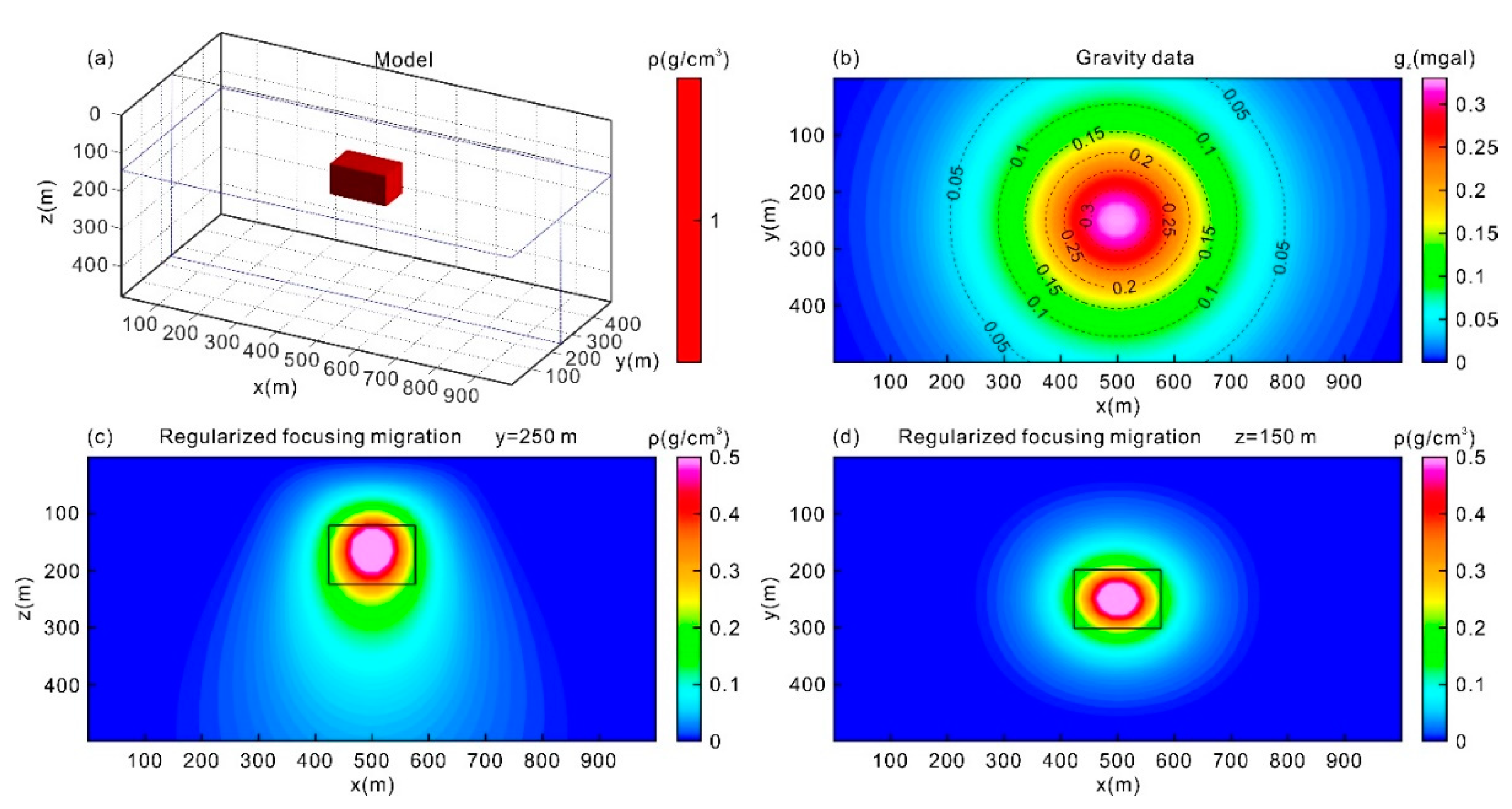
We examined the feasibility and effectiveness of 3D regularized focusing migration with several typical synthetic models. First, we designed a single cube with a density contrast of 1 g/cm3, with the center located at a depth of 150 m. The three-dimensional view of the subsurface model and its surface gravity anomalies are shown in Figure 2a,b. The subsurface inversion domain was divided into 50 × 50 × 25 regular cells.
Figure 2c,d show the cross-sections through the density volume resulting from the regularized focusing migration at y = 250 m and z = 150 m, respectively. The density extremum of the imaging results corresponded well with the center of the anomalous body, and the high-density distribution precisely outlined the anomalous body, which demonstrated the feasibility of the method.
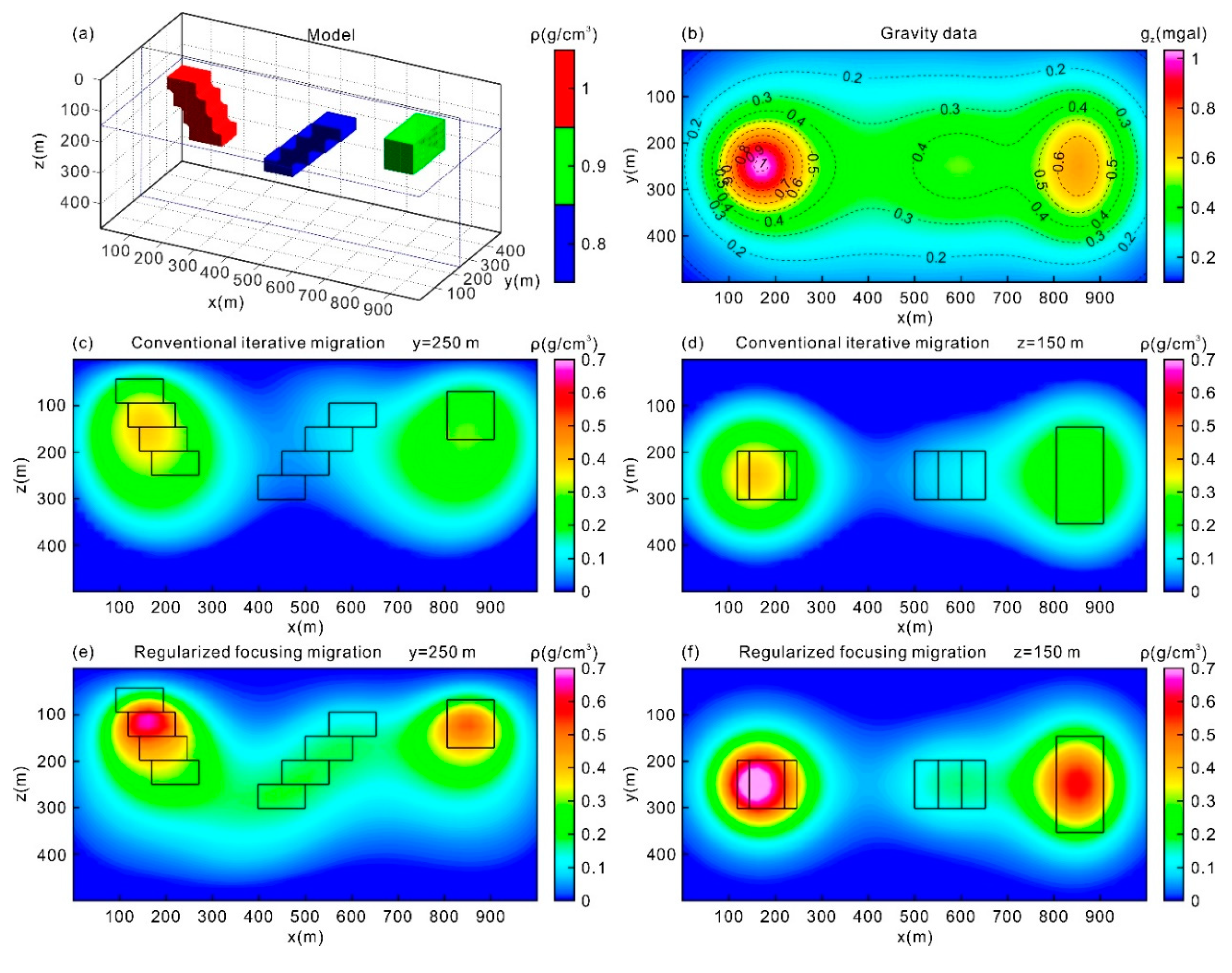
Our second synthetic example includes three anomalous bodies representing a dike complex and a prism (Figure 3a). Figure 3b shows the gravity anomaly computed by that model.
Figure 3c,f show the cross-sections of density distribution obtained by conventional iterative migration and regularized focusing migration. Regularized focusing migration method was able to distinguish the trends in the individual dikes, resulting in better convergence and a more realistic output, while better imaging the deep part of the model. However, the conventional iterative migration method barely distinguished three anomalous bodies and underestimated the dips in the modeled dikes, showing divergent density distribution that was far beyond the actual extent. In contrast, 3D regularized focusing resulted in a better spatial resolution and preserved sharper and finer boundaries.
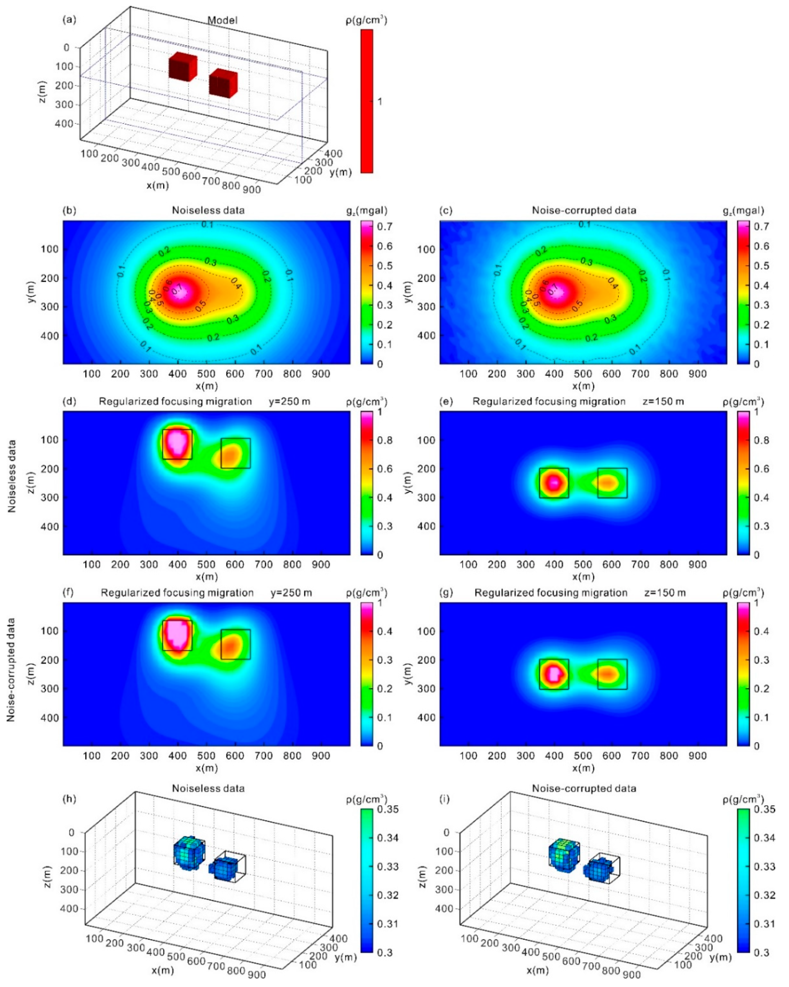
Next, we investigated how regularized focusing migration performs in noise conditions. Figure 4a shows the three-dimensional diagram for two isolated cubes with a density contrast of 1 g/cm3, located at depths of 70 m and 100 m. Figure 4b shows the surface gravity anomalies for this model. We added 5% random Gaussian noise to the observed gravity data, as shown in Figure 4c to simulate the data collected in actual surveys. The imaging results for noiseless and noise-corrupted data are shown in Figure 4d,g. The imaging results for both noiseless and noise-corrupted data were in good agreement with the true model. Although the two bodies were close in distance, which was equal to their side length, our method still distinguished the discrete bodies. The extremum of the derived density distribution corresponded well to the center of each geological body, and the horizontal positions and buried depths could be clearly delineated. However, the recovered density values were somewhat different from the actual conditions, especially for the deeper bodies. This is because the gravity field declines rapidly with depth, as shown in Equation (3). It is clear that the direct imaging of noise-containing data was still able to produce stable and smooth results. The volume images with a density cut-off greater than 0.3 g/cm3 of noiseless and noise-containing data, are also shown in Figure 4h,i, respectively. The result of the direct migration of noise-containing data is very similar to that of noiseless data. Based on the results of this test, we concluded that the regularized focusing migration method has good noise resistance since the introduction of a regularization term prevents local overfitting. This method shows good performance and is able to obtain the global optimal results.
We also analyzed the efficiency of the proposed method. All tests were run on an Intel Xeon E5-2650 (Intel, Santa Clara, CA, USA) with 2.2 Ghz, 64GB of main memory. The model shown in Figure 2a was adopted for this purpose. 
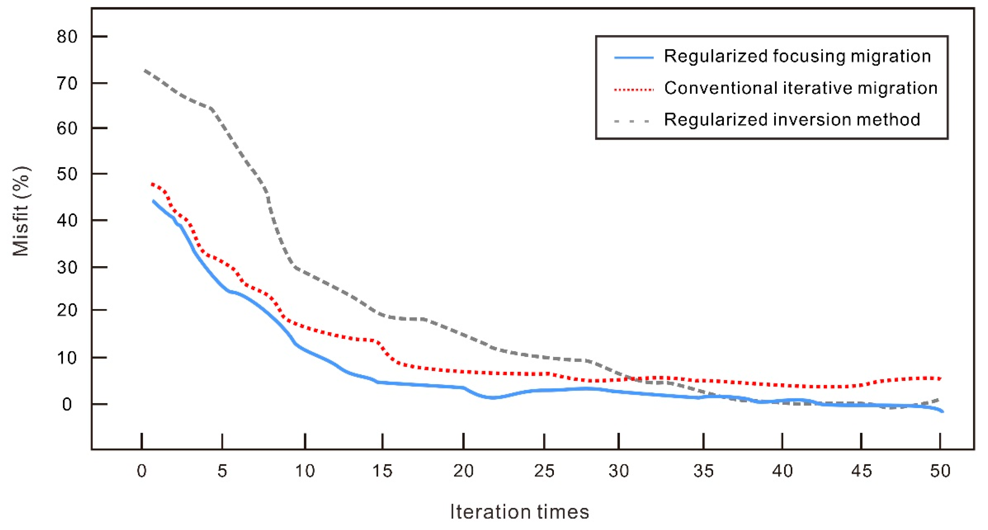
Figure 5 shows the misfit curves as a function of the number of iterations for the regularized inversion [32], the conventional iterative migration method and our proposed method. The migration method obtains a result with a lower misfit in the first iteration, which gives rise to convergence and less calculation time. Numerical results show that the migration method can decrease the iterative number by 35% compared with the inversion method and greatly reduce the computation time.
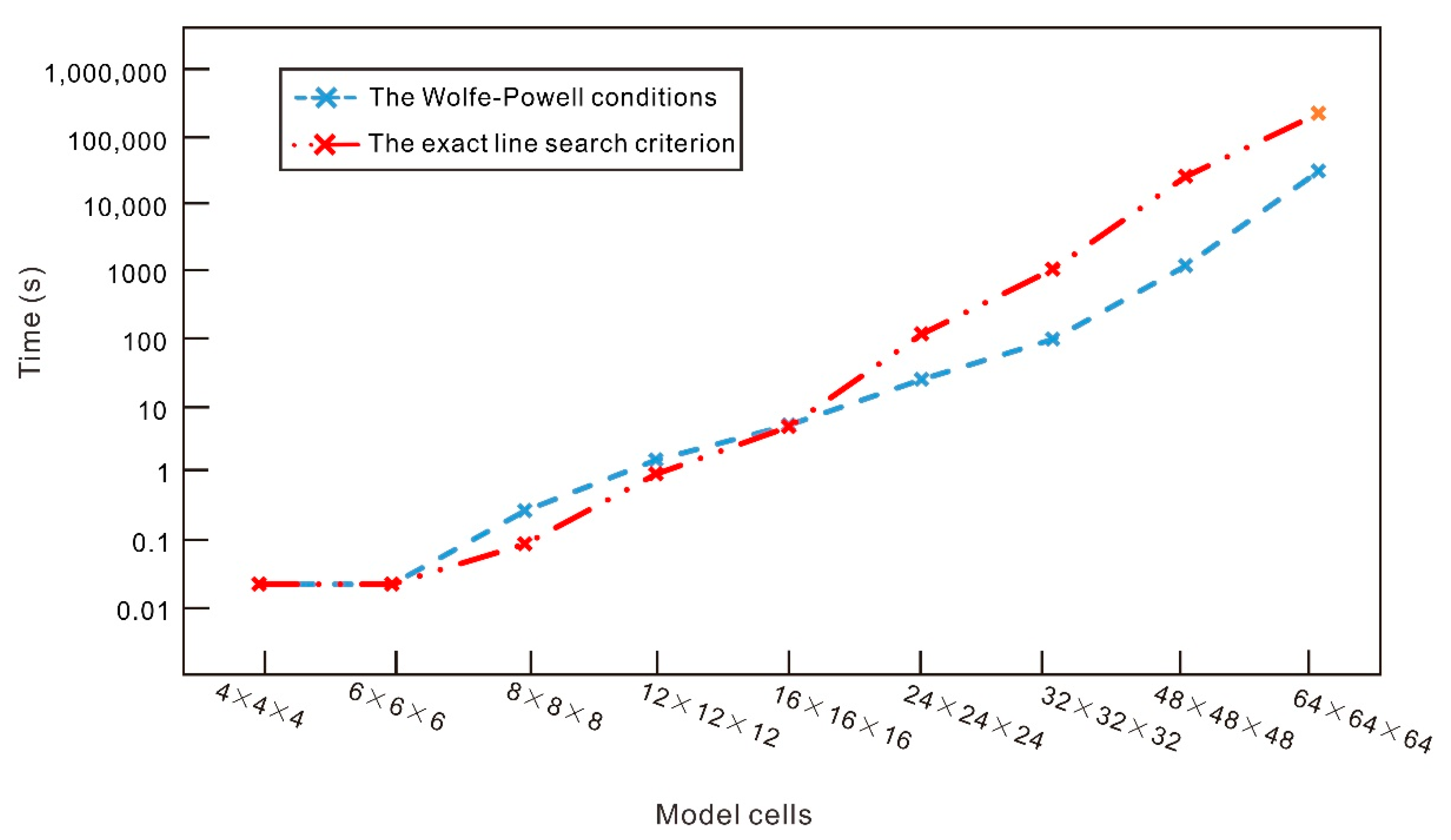
Figure 6 shows the computation time of the regularized focusing migration method as a function of the model scale. The iteration process stopped when the misfit calculated by Equation (31) reached 5%. For models less than 6 × 6 × 6 cells, the computation time for both line search criterion is constant because the model scale is relatively small and most of the time is spent on the initialization of the work. For models larger than 6 × 6 × 6 cells, computation time is linearly dependent on the scale of the model. For computations based on the Wolfe–Powell conditions, the time that is consumed is higher than that of the exact line search with models under 16 × 16 × 16 cells, but this is the opposite for the models exceeding 16 × 16 × 16 cells. This is because the exact line search for each step involves the calculation of A ω A ω * , which means that the time complexity grows roughly as ( n x . n y ) 2 ( n x . n y . n z ) 2 , while for the Wolfe–Powell conditions, which calculate A ω m multiple times, each time the step size is determined, the time complexity is approximately n x 2 n y 2 n z . The solution to the underdetermined system of equations does not depend on the exact search process. When the model scale is too large, the cost of using the exact line search is relatively high. According to the Wolfe–Powell conditions, the global convergence is expected to be fast. Although the number of steps increases, the convergence speed is accelerated.
To process the model with 50 × 50 × 25 cells, the runtime for our method was only 224 s compared to 2278 s for the conventional migration method and 1.8 h for the regularized inversion method. This efficiency is due to the adoption of the conjugate migration direction and the step size is based on the Wolfe–Powell conditions when the model parameters are updated during each iteration. Besides, the continuous decrease in the regularization parameter and the introduced focusing weight can also accelerate the convergence and obtain a solution that minimizes the objective functional more quickly. Therefore, when studying the regional structures and the deep geological problems, regularized focusing migration imaging can be used for global analysis without the need for data thinning. This is especially applicable to the investigation of large-scale mining areas, as in the following case study of the Yucheng mining area, Dezhou, Shandong, China.

4. Field Example

In 2011, the Shandong Province Mineral Resources Potential Evaluation Project revealed that the Yucheng area had metallogenic conditions that are indicative of skarn-type ore deposits. In the following years, a variety of geological surveys showed that the area had good prospecting potential, and the iron ore bodies were confirmed during drilling. The traditional interpretation of the geophysical surveys in this area was based on the analysis of gravity or magnetic anomalies in contour maps [33,34,35], which provided the major geophysical characteristics of the area and was used to determine the approximate extent of the deposits. However, they alone could not determine the exact locations and depths of the mineral deposits.
In the following sections, we first summarize the metallogenic geological conditions of this area, then use our high-resolution method to invert the results of the entire airborne gravity data into 3D density models, and finally, we analyze the density imaging results to identify potential mining targets. Our work provides a reference for follow-up studies and further exploration of skarn-type iron ore under a thick overburden.

4.1. Geological Background of the Survey Area

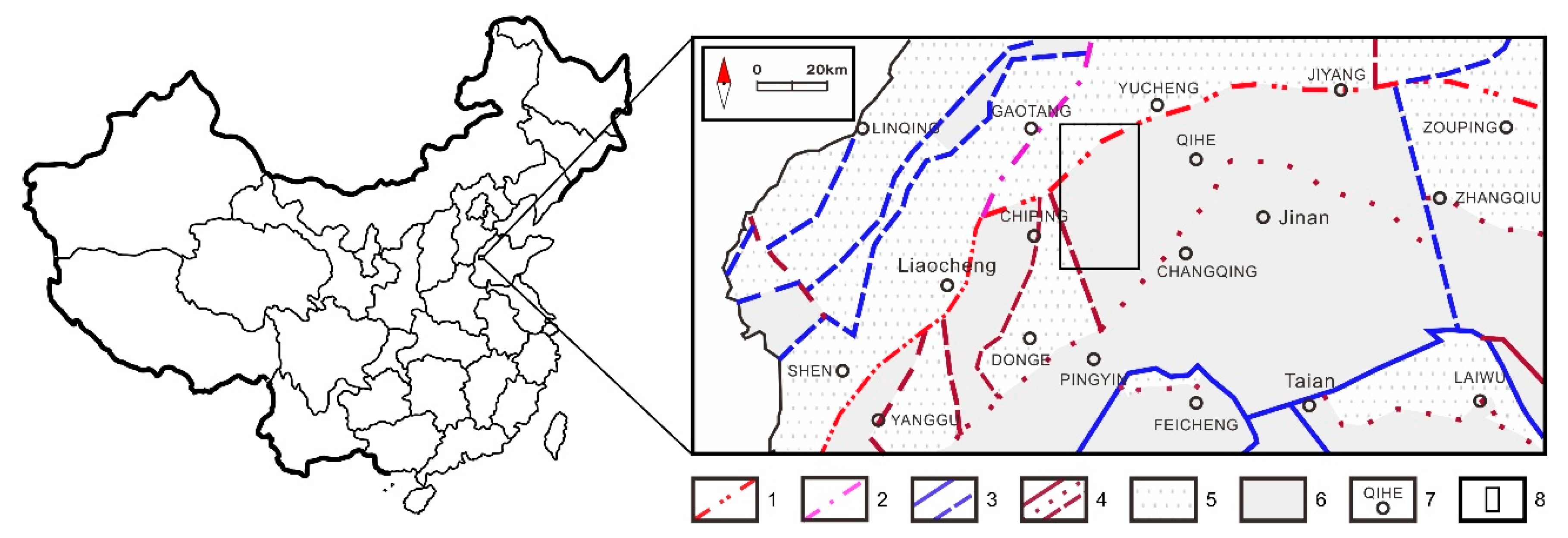
The survey area is located near the Qihe county and Yucheng county borders to the south of Dezhou city in Shandong province, and belongs to the northwestern Shandong plain. It is located in the Luxi uplift area of the North China tectonic plate (Figure 7) [36]. The area is covered by strata of Cambrian, Ordovician, Carboniferous, Permian, Neogene and Quaternary from the base to the top [33]. The surface is completely covered by thick Quaternary and Neogene strata without any bedrock outcrops [37]. All kinds of deep geological information can be inferred from geophysical data. Due to regional tectonic movements, fault structures are widespread, including NE-striking faults, NNW-striking faults and SN-striking faults, and local developed fold structures (Figure 8).
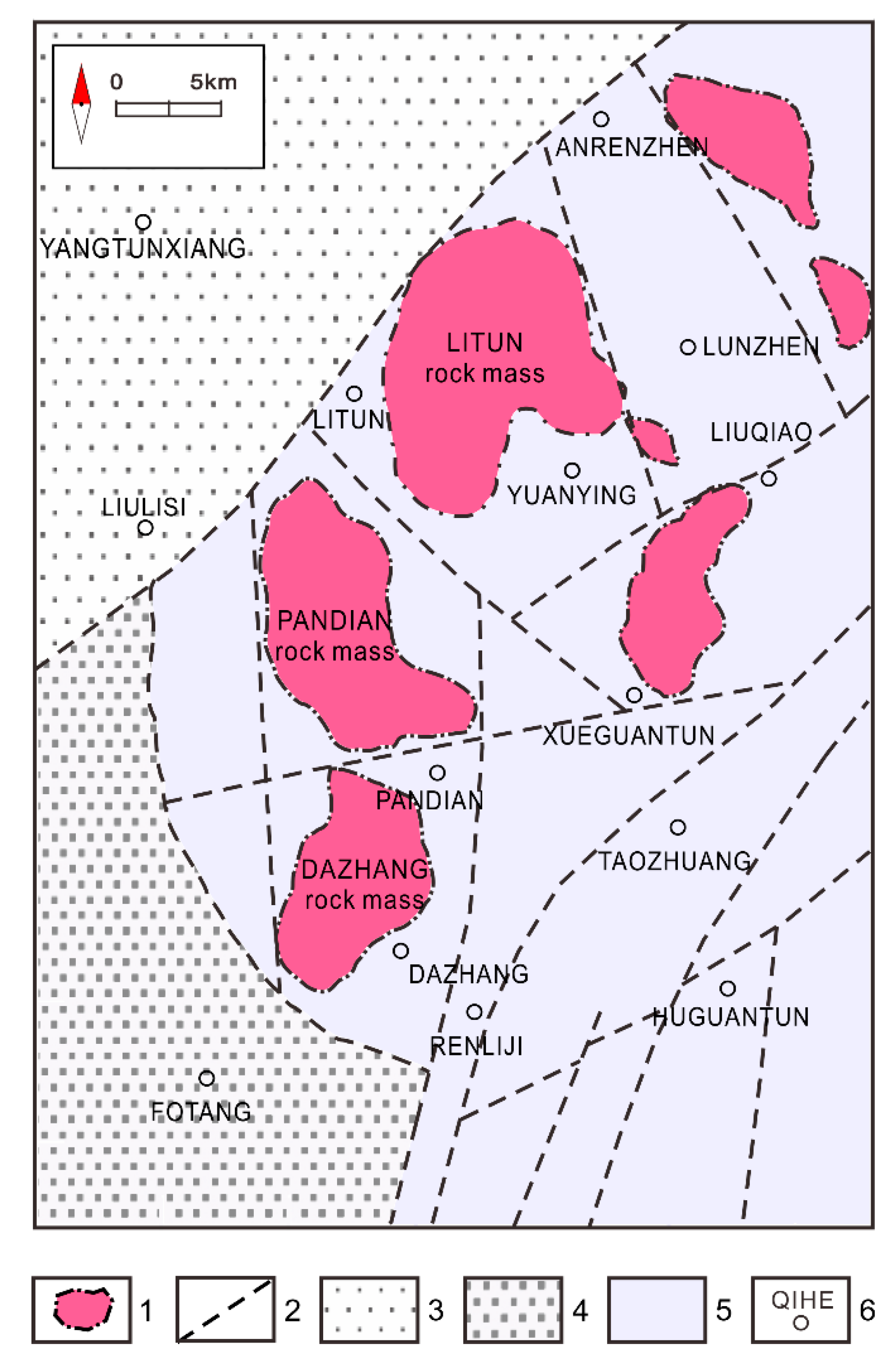
The carbonate rocks of the Ordovician Majiagou group are widely distributed and serve as host rocks for skarn-type iron ores. In addition, some iron-ore bodies also occur in the clastic rocks of the Carboniferous-Permian group. According to available borehole data, the depth of the Ordovician strata in the northwest reaches 3440 m or more, whereas it varies greatly in the southeastern area, ranging from 1165 m and 610–650 m in the east of Litun and in the northwest of Dazhang, respectively. There is no borehole data for the northwest of Pandian, and the depth of the Ordovician rocks is unknown [36]. In the survey area, magmatic activity was intense during the late Yanshanian period, and a significant volume of igneous rock mass was added at that time. The investigation of iron ores indicates that the ore bodies occur near the contact zone between the body mass of the late Yanshanian intermediate-basic intrusive rocks that are dominated by diorite and gabbro and the state of Ordovician limestone. In addition, a small number of ore bodies occur near the intersection of fault structures and in the xenoliths near the rock mass [35].

4.2. Data Acquisition

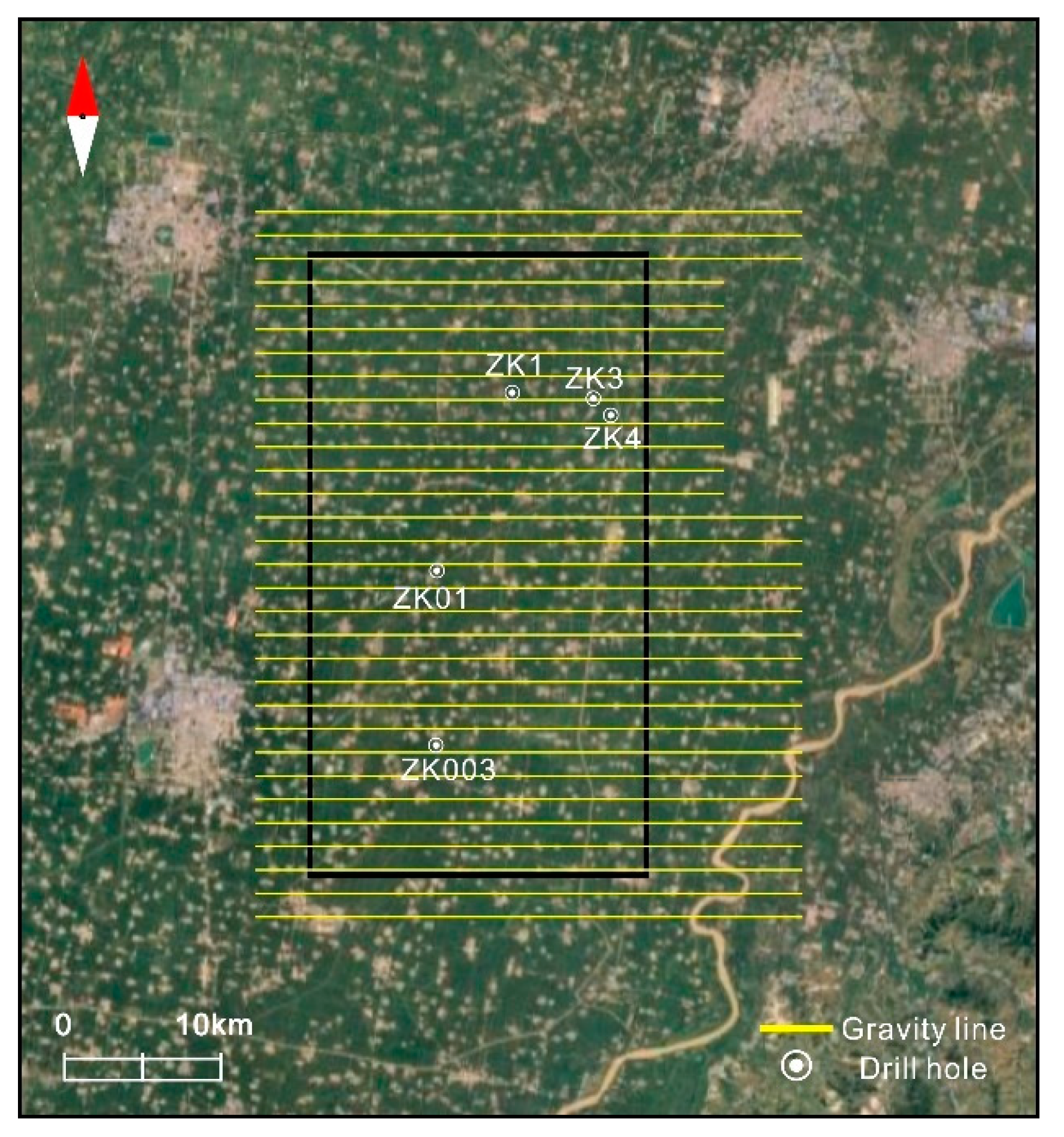
The airborne gravity survey that collected gravity data in the Yucheng area, Shandong was performed by the China Aero-Geophysical Survey and Remote Sensing Center for Land and Resources (AGRS, Beijing, China). During the survey, a gravimeter was installed in the cabin of a CESSNA208 aircraft. The flight altitude was fixed at 450 m above sea level. The 45 × 35 km2 survey area was flown at line spacings of 1500 m. The flight survey lines were designed to be perpendicular to the regional geological strike to ensure effective sampling. Figure 9 shows the gravity survey lines in the Yucheng area and the black rectangle delineates the region where we perform regularized focusing migration.

4.3. Migration Models of Gravity Data

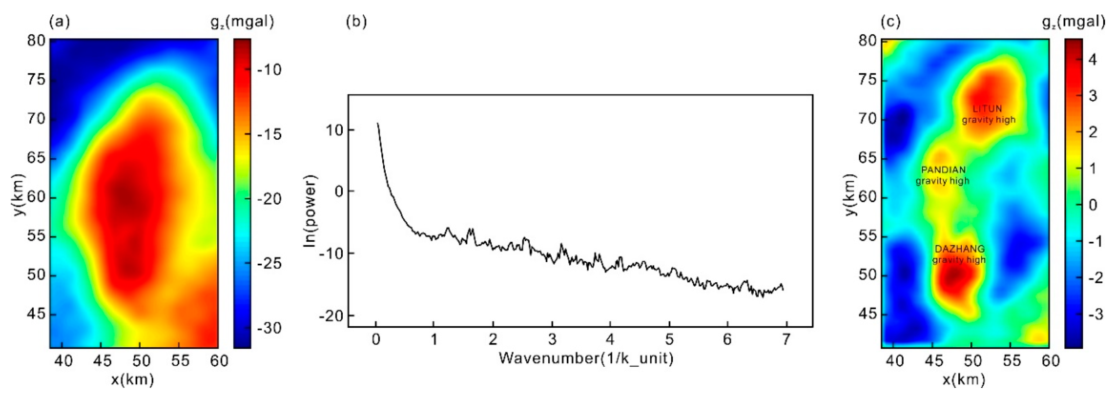
We performed a terrain correction, latitude correction, and Bouguer correction on the collected gravity data to obtain Bouguer gravity anomalies (Figure 10a). The characteristics of regional gravity anomalies generally reflected the distribution of late Yanshanian intrusive rocks and the Ordovician strata uplift in the region. The iron-ore deposits of interest are shallower than 2 km because the iron ores below that have no economic mining value. The regional field below 2 km was separated from the Bouguer gravity anomaly by matched filtering [38], thus weakening the influence of deep structures on the imaging results for shallow density migration. Figure 10b shows the radial logarithmic power spectrum of the Bouguer gravity anomalies. Long-wavelength anomalies were removed to obtain the shallow local gravity anomalies. Figure 10c shows the local gravity anomalies, where three gravity highs can be seen. Four wells were drilled, including three holes in the Litun area and one hole in the Yucheng area, and the ZK1 well in the Litun area and the ZK003 well in the Dazhang area discovered bodies of rich magnetite (Table 1 and Table 2). According to borehole data, the density of magnetite was significantly higher than other rocks.
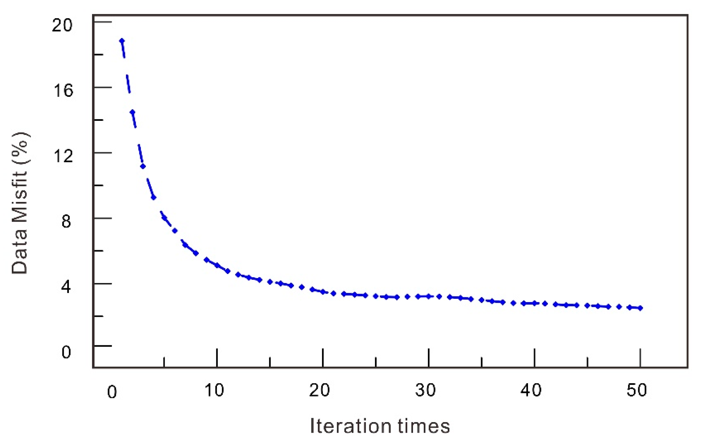
Based on the characteristics of the stratigraphic, magmatic rocks distribution and the drilling data in the survey area, the high value of the local gravity anomalies were mainly caused by the skarn-type magnetite deposits. The positive density contrast of the migration imaging results could be used as a prospecting criterion. We performed regularized focusing migration imaging of local gravity anomalies with an initial model based on drilling data, and then delineated the spatial distribution of the iron ore under the range of positive density contrast of the imaging results. The local gravity data were inverted in a region designed as 21,500 m × 39,600 m in the X and Y directions and 2 km in the Z direction, with 88 × 98 × 50 small cells. Figure 11 shows the convergence curve of the migration. 
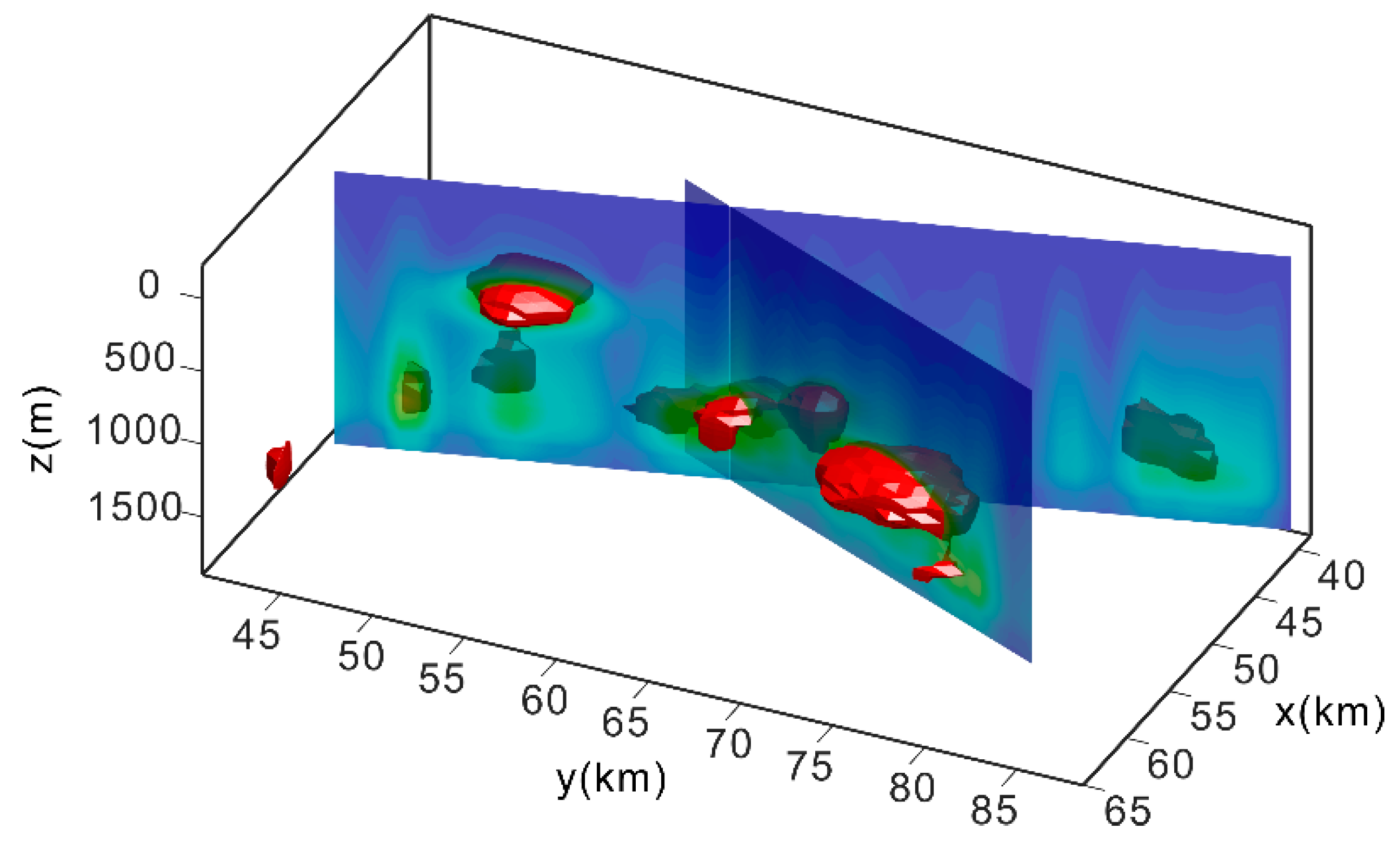
Figure 12 shows a perspective view of the migration density model with abnormal parts with a density greater than 0.7 g/cm
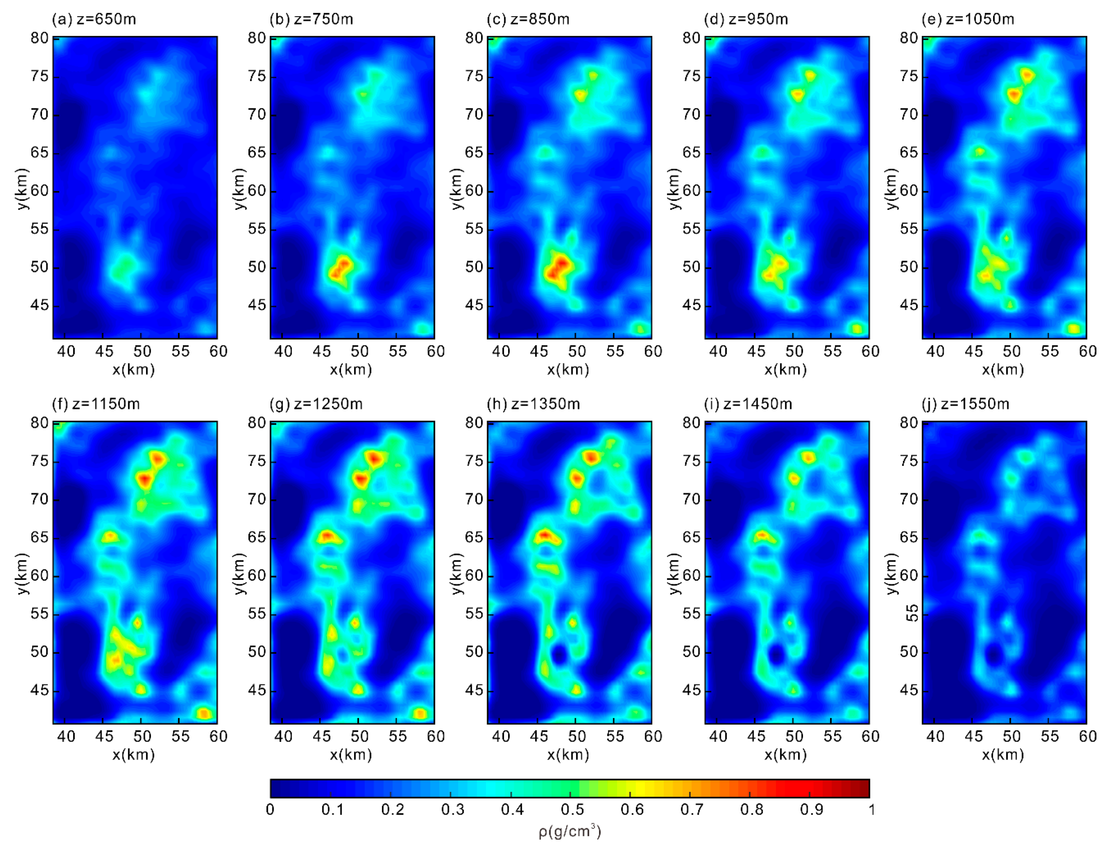
3, which gives a clear view of the anomalous bodies. For a better representation, several horizontal cross-sections with different depths are shown in Figure 13.

4.4. Geological Interpretation of the Mining Area

The results of migration imaging suggest that there are considerable mineral resources underneath the Litun, Pandian and Dazhang anomaly areas. Ore bodies derived from our analysis are mainly distributed between a depth of 700 m and 1500 m.
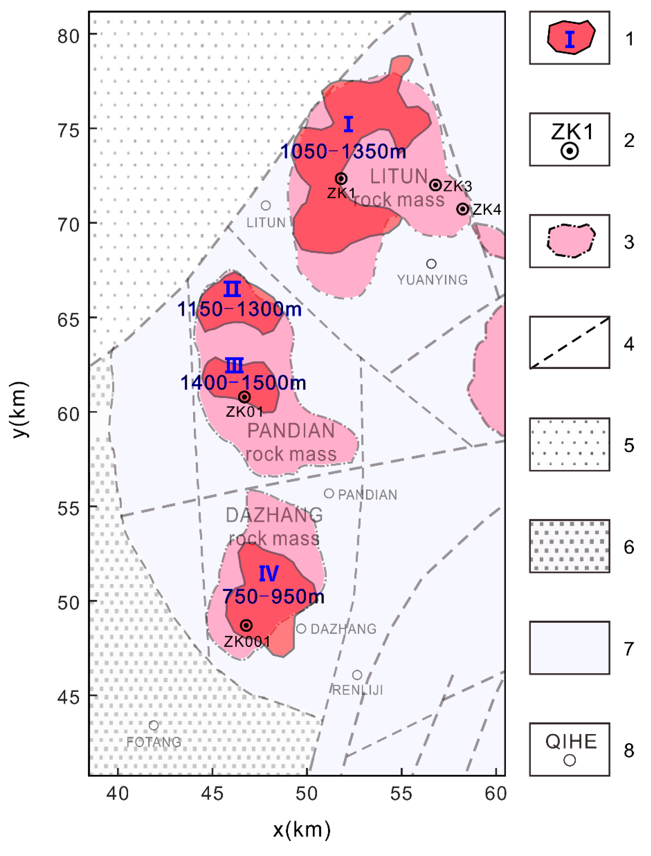
Figure 14 shows the ore-body distribution superimposed on a simplified geological map of the survey area. One can see that the target mineralized zones are mainly concentrated in the vicinity of fault structures since faults can provide channels for magmatic upwelling. The iron ore in Litun (I) is buried at a depth of about 1050–1350 m, that in Pandian (II, III) is about 1150–1550 m deep, and that in Dazhang (IV) is about 750–950 m. It should be noted that the Pandian area (II, III) is rich in iron ore resources underground, but these resources are deeper and less extensive, and drilling would be more difficult than in the Litun (I) and Dazhang areas (IV). The iron ores in the Litun and Dacheung areas are characterized by their great thickness, shallow burial and easy mining, and these should be regarded as key prospecting drilling areas. When these targets are exhausted and more geological information is obtained, exploration can proceed outward, including under the Pandian area along with other nearby high-density distributions that have not yet been measured.
The recent well (ZK01) in this area found a body of ore that is 54.4 m thick at a depth of 1444.4 m, which is consistent with our interpretation. Therefore, the regularized focusing migration method has the ability to delineate the horizontal range of the ore body, predict its mineral depth and summarize prospecting targets.

5. Conclusions

Here, we developed 3D regularized focusing migration of large-scale gravity data with higher horizontal and vertical resolution than conventional gravity migration imaging. As validated by synthetic models, this method can determine complicated geological structures and it has high stability in noise conditions. Furthermore, the proposed algorithm based on the conjugate migration direction and the Wolfe–Powell conditions inherits the high efficiency of conventional migration and can produce real-time imaging with high accuracy. This provides a method that can delineate deep mineral resources.
We have shown how this method was efficiently used for the interpretation of the airborne gravity data collected over the Yucheng mining area, Dezhou, Shandong, China. High-resolution imaging results were obtained for the high-density body distribution, which helped to identify several potential mining targets with no surface expression. Currently, one of the predicted targets outlined in our study is undergoing further drilling exploration based on these airborne gravity analyses and well results so far coincide with our predictions. This method offers a basis for further exploration in this area to map the skarn-type iron-ore bodies under a thick overburden.
Gravity and magnetic combination migration will be used further in this area to reduce the non-uniqueness of the results. Joint migration of multiple geophysical data is the focus of our future research.

Author Contributions

Conceptualization, Y.D. and G.M.; data curation, Y.D. and G.M.; formal analysis, Y.D.; funding acquisition, G.M.; investigation, Y.D.; methodology, Y.D.; project administration, G.M.; resources, S.X.; software, Y.D. and H.W.; supervision, G.M.; validation, Y.D.; visualization, Y.D.; writing—original draft, Y.D.; writing—review & editing, G.M. All authors have read and agreed to the published version of the manuscript.

Funding

This research was funded by the National Key Research and Development Program of China, grant numbers 2017YFC0602203 and 2017YFC0602000.

Conflicts of Interest

The authors declare no conflict of interest.

References

  1. Tikhonov, A.N. Regularization of incorrectly posed problem. Sov. Math. Dokl. 1963, 4, 1624–1627. [Google Scholar]
  2. Phillips, D.L. A technique for the numerical solution of certain integral equations of the first kind. J. ACM 1962, 9, 84–97. [Google Scholar] [CrossRef]
  3. Strakhov, V.N. The solution of linear ill-posed problems in Hilbert space. Differ. Uravn. 1970, 6, 1490–1495. [Google Scholar]
  4. Lavrent’ev, M.M.; Romanov, V.G.; Shishatskii, S.P. Ill—Posed Problems of Mathematical Physics and Analysis, 1st ed.; American Mathematical Society: Providence, RI, USA, 1986; pp. 290–299. [Google Scholar]
  5. Tikhonov, A.N.; Arsenin, V.Y. Solutions of Ill—Posed Problems; Wiley: Hoboken, NJ, USA, 1977. [Google Scholar]
  6. Zhdanov, M.S. Geophysical Inverse Theory and Regularization Problems, 1st ed.; Elsevier: Amsterdam, The Netherlands, 2002; Volume 36, pp. 42–186. [Google Scholar]
  7. Zhdanov, M.S. Inverse Theory and Applications in Geophysics, 2nd ed.; Elsevier: Amsterdam, The Netherlands, 2015; Volume 36, pp. 46–172. [Google Scholar]
  8. Zhang, R.; Li, T.; Zhou, S.; Deng, X. Joint MT and gravity inversion using structural constraints: A case study from the Linjiang copper mining area, Jilin, China. Minerals 2019, 9, 407. [Google Scholar] [CrossRef] [Green Version]
  9. Li, Y.; Oldenburg, D.W. 3-D inversion of gravity data. Geophysics 1998, 63, 109–119. [Google Scholar] [CrossRef]
  10. Li, Y. 3-D inversion of gravity gradiometer data. In SEG Technical Program Expanded Abstracts; Society of Exploration Geophysicists: Tulsa, OK, USA, 1999; pp. 1470–1473. [Google Scholar]
  11. Van Zon, T.; Roy-Chowdhury, K. Structural inversion of gravity data using linear programming. Geophysics 2006, 71, 41–50. [Google Scholar] [CrossRef]
  12. Martins, C.M.; Lima, W.A.; Barbosa, V.C.; Silva, J.B. Total variation regularization for depth-to-basement estimate: Part 1—Mathematical details and applications. Geophysics 2011, 76, I1–I12. [Google Scholar] [CrossRef]
  13. Lima, W.A.; Martins, C.M.; Silva, J.B.; Barbosa, V.C. Total variation regularization for depth-to-basement estimate: Part 2—Physicogeologic meaning and comparisons with previous inversion methods. Geophysics 2011, 76, I13–I20. [Google Scholar] [CrossRef]
  14. Last, B.J.; Kubik, K. Compact gravity inversion. Geophysics 1983, 48, 713–721. [Google Scholar] [CrossRef]
  15. Portniaguine, O.; Zhdanov, M.S. Focusing geophysical inversion images. Geophysics 1999, 64, 874–887. [Google Scholar] [CrossRef] [Green Version]
  16. Farquharson, C.G.; Oldenburg, D.W. A comparison of automatic techniques for estimating the regularization parameter in non-linear inverse problems. Geophys. J. Int. 2004, 156, 411–425. [Google Scholar] [CrossRef] [Green Version]
  17. Wahba, G. Spline models for observational data. Technometrics 1990, 34, 113–114. [Google Scholar]
  18. Hansen, P.C. Rank-Deficient and Discrete Ill—Posed Problems: Numerical Aspects of Linear Inversion, 2nd ed.; Society for Industrial and Applied Mathematics: Philadelphia, PA, USA, 1998; pp. 69–87. [Google Scholar]
  19. Liu, S.; Baniamerian, J.; Fedi, M. Imaging Methods versus inverse methods: An option or an alternative? IEEE Trans. Geosci. Remote Sens. 2020, 58, 3484–3494. [Google Scholar] [CrossRef]
  20. Zhdanov, M.S.; Liu, X.; Wilson, G.A. Rapid imaging of gravity gradiometry data using 2D potential field migration. In SEG Technical Program Expanded Abstracts; Society of Exploration Geophysicists: Tulsa, OK, USA, 2010; pp. 1132–1136. [Google Scholar]
  21. Zhdanov, M.S.; Liu, X.; Wilson, G. Potential field migration for rapid 3D imaging of entire gravity gradiometry surveys. First Break 2010, 28, 47–51. [Google Scholar] [CrossRef]
  22. Zhdanov, M.S.; Liu, X.; Wan, L.; Čuma, M.; Wilson, G.A. 3D potential field migration for rapid imaging of gravity gradiometry data—A case study from Broken Hill, Australia, with comparison to 3D regularized inversion. In SEG Technical Program Expanded Abstracts; Society of Exploration Geophysicists: Tulsa, OK, USA, 2011; pp. 825–829. [Google Scholar]
  23. Zhdanov, M.S.; Liu, X.; Wilson, G.A.; Wan, L. Potential field migration for rapid imaging of gravity gradiometry data. Geophys. Prospect. 2011, 59, 1052–1071. [Google Scholar] [CrossRef]
  24. Wan, L.; Zhdanov, M.S. Iterative migration of gravity and gravity gradiometry data. In SEG Technical Program Expanded Abstracts; Society of Exploration Geophysicists: Tulsa, OK, USA, 2013; pp. 1211–1215. [Google Scholar]
  25. Wan, L.; Han, M.; Zhdanov, M.S. Joint iterative migration of surface and borehole gravity gradiometry data. In SEG Technical Program Expanded Abstracts; Society of Exploration Geophysicists: Tulsa, OK, USA, 2016; pp. 1607–1611. [Google Scholar]
  26. Wolfe, P. Convergence conditions for ascent methods. SIAM Rev. 1969, 11, 226–235. [Google Scholar] [CrossRef]
  27. Powell, M.J.D. Some Global Convergence Properties of a Variable Metric Algorithm for Minimization without Exact Line Searches, 1st ed.; SIAM publications: Philadelphia, PA, USA, 1976; pp. 53–72. [Google Scholar]
  28. Forsberg, R.; Tscherning, C.C. The use of height data in gravity field approximation by collocation. J. Geophys. Res. Solid Earth 1981, 86, 7843–7854. [Google Scholar] [CrossRef]
  29. Zhdanov, M.S.; Tolstaya, E. Minimum support nonlinear parametrization in the solution of a 3D magnetotelluric inverse problem. Inverse Probl. 2004, 20, 937. [Google Scholar] [CrossRef]
  30. Lemaréchal, C. A view of line-searches. In Optimization and Optimal Control, 1st ed.; Springer: Berlin/Heidelberg, Germany, 1981; pp. 59–78. [Google Scholar]
  31. Portniaguine, O.; Zhdanov, M.S. 3-D magnetic inversion with data compression and image focusing. Geophysics 2002, 67, 1532–1541. [Google Scholar] [CrossRef] [Green Version]
  32. Zhdanov, M.S.; Ellis, R.; Mukherjee, S. Three-dimensional regularized focusing inversion of gravity gradient tensor component data. Geophysics 2004, 69, 925–937. [Google Scholar] [CrossRef]
  33. Cheng, X.; Wang, J.; Wang, J.; Zhai, D.; Cai, T. Geological characteristics and prospecting potential of Dazhang iron deposit in Qihe County of Shangdong Province. Shandong Land Resour. 2017, 33, 24–29. [Google Scholar]
  34. Guo, Y.; Hao, X.; Zhong, W.; Ru, L.; Zhao, C. Application of high-precision magnetic measurement in exploration of hidden iron deposit: Setting iron deposits in Litun area of Yuchen City in Shandong Province as an example. Shandong Land Resour. 2017, 33, 52–56. [Google Scholar]
  35. Hao, X.; Yang, Y.; Li, Y.; Gao, H.; Chen, L. Ore-controlling characteristics and prospecting criteria of iron deposits in Qihe area of western Shandong. J. Jilin Univ. 2019, 49, 982–991. [Google Scholar]
  36. Kong, Q.; Zhang, T. Deposits of Shandong, 1st ed.; Shandong Science and Technology Press: Jinan, China, 2006; pp. 64–71. [Google Scholar]
  37. Hao, X.; Liu, W.; Zang, K.; Zhang, X. Primary study on metallogenic regularity of skarn type iron deposit in Pandian area in western Shandong Province. Shandong Land Resour. 2018, 34, 27–33. [Google Scholar]
  38. Syberg, F.J.R. A Fourier method for the regional—Residual problem of potential fields. Geophys. Prospect. 1972, 20, 47–75. [Google Scholar] [CrossRef]
Figure 1. Representation of the subsurface density distribution. (a) A layer of rectilinear cuboids; (b) a single cuboid. The observation position is described by coordinate ( x ,   y ,   z ) . The coordinates of cuboid corners can be completely described by two vertices ( ε 1 ,   η 1 ,   ζ 1 ) and ( ε 2 ,   η 2 ,   ζ 2 ) .
Minerals 10 00471 g001
Figure 2. (a) Three-dimensional view of a single cube model; (b) gravity anomalies at z = 0 m generated from the model; (c) vertical cross-section of y = 250 m obtained from 3D regularized focusing migration; (d) horizontal cross-section of z = 150 m obtained from 3D regularized focusing migration.
Minerals 10 00471 g002
Figure 3. (a) Three-dimensional view of the subsurface model; (b) gravity anomalies at z = 0 m generated from the model; (c) vertical cross-section of y = 250 m obtained from conventional iterative migration; (d) horizontal cross-section of z = 150 m obtained from conventional iterative migration; (e) vertical cross-section of y = 250 m obtained from 3D regularized focusing migration; and (f) horizontal cross-section of z = 150 m obtained from 3D regularized focusing migration.
Minerals 10 00471 g003
Figure 4. (a) Three-dimensional view of the subsurface model; (b) gravity anomalies at z = 0 m generated from the model; (c) gravity anomalies at z = 0 m generated from the model with 5% random Gaussian noise added; (d) vertical cross-section of y = 250 m for noiseless gravity data; (e) horizontal cross-section of z = 150 m for noiseless gravity data; (f) vertical cross-section of y = 250 m for noise-corrupted data; (g) vertical cross-section of z = 150 m for noise-corrupted data; (h) volume image with a density cut-off greater than 0.3 g/cm3 for noiseless data; (i) volume image with a density cut-off greater than 0.3 g/cm3 for noise-corrupted data.
Minerals 10 00471 g004
Figure 5. Misfit of three different methods: regularized focusing migration, conventional iterative migration and regularized inversion.
Minerals 10 00471 g005
Figure 6. Computation time of regularized focusing migration method for models of different sizes. The blue line represents use of the Wolfe–Powell line search conditions as shown in Equations (24)–(26), and the red line represents use of the exact line search criterion as shown in Equation (9).
Minerals 10 00471 g006
Figure 7. Tectonic background map of Yucheng area. The survey area is detailed in the black rectangle. 1 = the secondary structural unit; 2 = the tertiary structural unit; 3 = the quaternary structural unit; 4 = five-level structural unit; 5 = (latent) sag zone; 6 = (latent) high zone; 7 = toponym; 8 = survey area.
Minerals 10 00471 g007
Figure 8. Geological map of the survey area. The figure is from [36]. 1 = Inferred range of concealed diorite rocks; 2 = inferred concealed fault; 3 = Yucheng-Jiyang latent sag; 4 = Lepingpu latent sag; 5 = Qihe latent high; and 6 = toponym.
Minerals 10 00471 g008
Figure 9. Gravity survey lines in the Yucheng area. The black rectangle shows the region used for regularized focusing migration.
Minerals 10 00471 g009
Figure 10. (a) Regional gravity anomaly; (b) radial logarithmic power spectrum; (c) local gravity anomaly.
Minerals 10 00471 g010
Figure 11. Convergence curve of the migration.
Minerals 10 00471 g011
Figure 12. Perspective view of the migration density model. The red anomalous bodies show a density distribution with density greater than 0.7 g/cm3.
Minerals 10 00471 g012
Figure 13. Horizontal cross-sections at (a) z = 650 m, (b) z = 750 m, (c) z = 850 m, (d) z = 950 m, (e) z = 1050 m, (f) z = 1150 m, (g) z = 1250 m, (h) z = 1350 m, (i) z = 1450 m and (j) z = 1550 m of imaging results.
Minerals 10 00471 g013
Figure 14. Map of iron ore range co-rendered with the corresponding geological map. 1 = scope of prospecting target area; 2 = drill hole; 3 = inferred range of concealed diorite rocks; 4 = inferred concealed fault; 5 = Yucheng-Jiyang latent sag; 6 = Lepingpu latent sag; 7 = Qihe latent high; 8 = toponym.
Minerals 10 00471 g014
Table 1. Dazhang ZK003 drilling data.
LithologyTop Surface Depth (m)Thickness (m)Density (g/cm3)
Sand/mealy sand/clay0571.9
Mudstone/sandstone/limestone571.918.42.69
Limestone590.319.12.68
Limestone609.4103.72.72
Diorite713.186.32.64
Skarn799.42.63.15
Magnetite80215.34.41
Skarn817.32.43.18
Magnetite819.70.64.45
Diorite820.3105.72.63
Table 2. Litun ZK1 drilling data.
LithologyTop Surface Depth (m)Thickness (m)Density (g/cm3)
Sandstone/mudstone01126.19
Diorite1126.1919.032.57
Skarn dolomite1145.225.022.66
Skarn 1150.247.142.87
Magnetite1157.389.344.19
Skarn1166.723.152.82
Magnetite1169.878.774.26
Crushed zone1178.645.31
Skarn1183.9514.392.84
Magnetite1198.3498.154.49
Skarn1296.4916.352.87
Diorite1312.64123.462.68

