Article

Process Variable Importance Analysis by Use of Random Forests in a Shapley Regression Framework

1
Western Australian School of Mines: Minerals, Energy and Chemical Engineering, Curtin University, GPO Box U1987, Perth, WA 6845, Australia
2
Department of Process Engineering, Stellenbosch University, Private Bag X1, Matieland, Stellenbosch 7602, South Africa
Minerals 2020, 10(5), 420; https://doi.org/10.3390/min10050420
Submission received: 29 March 2020 / Revised: 3 May 2020 / Accepted: 6 May 2020 / Published: 8 May 2020
(This article belongs to the Special Issue Novel Advanced Machine Learning Methods in Mineral Processing)

Abstract

:
Linear regression is often used as a diagnostic tool to understand the relative contributions of operational variables to some key performance indicator or response variable. However, owing to the nature of plant operations, predictor variables tend to be correlated, often highly so, and this can lead to significant complications in assessing the importance of these variables. Shapley regression is seen as the only axiomatic approach to deal with this problem but has almost exclusively been used with linear models to date. In this paper, the approach is extended to random forests, and the results are compared with some of the empirical variable importance measures widely used with these models, i.e., permutation and Gini variable importance measures. Four case studies are considered, of which two are based on simulated data and two on real world data from the mineral process industries. These case studies suggest that the random forest Shapley variable importance measure may be a more reliable indicator of the influence of predictor variables than the other measures that were considered. Moreover, the results obtained with the Gini variable importance measure was as reliable or better than that obtained with the permutation measure of the random forest.

1. Introduction

Insight into the underlying physical phenomena in process systems is key to the development of reliable process models. These models are in turn vital to the development of advanced process control systems and optimization of process operations. With the availability of large amounts of plant data becoming more commonplace, there is a growing interest in the use of operational data to gain deeper insights into process systems and plant operations [1].
Linear regression is well established as a diagnostic tool to understand the relative contributions or the statistical significance of operational variables to some key performance indicator or response variable on process plants. However, owing to the nature of plant operations, predictor variables tend to be correlated, and this can lead to significant complications in assessing the importance of these variables. Despite a number of methods that have been proposed to surmount the problem, Shapley regression is seen as the only axiomatic approach to deal with it [2,3,4]. As a consequence, linear Shapley regression models and variants thereof [2,5,6] have seen steady growth in application over the last few decades.
However, while linear models can be used to explicitly capture nonlinear process behavior, this would require a sound understanding of the underlying process phenomena, which may not be available. Although there is no reason why the same approach cannot be used with machine learning models in general, few, if any, such studies have been reported in the literature as yet. Therefore, in this paper, Shapley regression using random forests, instead of linear models, is investigated.
Random forests are a popular approach to develop reliable models for process systems. They are robust, i.e., they contain few hyperparameters to be specified by the user and can also be used to quantitatively assess the contributions of predictor variables to the response. These models have been used in variable importance analysis in a wide range of technical disciplines, including the mineral processing industries. Examples of these applications include the use of such models in comminution [7,8,9,10], froth flotation systems [11,12,13,14,15,16], sensor-based ore sorting [17], and blast fragmentation from open pit mines [18]. Most of these applications are comparatively recent, and this is a reflection of the rapid growth of random forests in mineral processing in the wake of similarly strong and continued growth in other disciplines.
The rest of the paper is organized as follows. In Section 2, Shapley regression as a methodology is introduced, followed by a brief overview of random forests in Section 3. Section 4 discusses the variable importance measures considered in the paper, as well as the use of random forests in a Shapley regression framework. This is followed by four case studies in Section 5. In Section 6, the results are discussed and the conclusions of the investigation are summarized.

2. Shapley Regression

2.1. Methodology

Shapley regression has its origin in game theory from the 1950s and has been reinvented multiple times with different terminology, including dominance analysis [5,19] and regression analysis in a game theory approach [2]. In essence, the fraction of the variance of the response variable explained by the model can be decomposed as indicated in Equation (1).
R j 2 = S V \ { x j } | S | ! ( m | S | 1 ) ! m ! [ R 2 ( S { x j } ) R 2 ( S ) ] .
If the m predictor variables are denoted by a set V = { x 1 , x 2 , x m } , then S is some subset of the set of predictor variables V and | S | is the number of elements in the set S . V \ { x j } is the set of predictor variables, excluding variable x j . R 2 ( S ) is the R 2 -value of the regression of the predictor variables in S on the response y and R j 2 is the marginal contribution of variable x 2 to the overall model R 2 -value. It is further assumed that R 2 ( ) = 0 .
The | S | ! ( m | S | 1 ) ! m ! term is a weight that compensates among other for the fact that variable coalitions generally differ in size. For example, if there are m = 3 variables ( A , B and C ), then S can either have 0, 1 or 2 elements. In this case, there are four coalitions to consider in the analysis of any single variable. For variable A , for example, the models to consider would be y = f ( A ) ,   y = f ( A , B ) ,   y = f ( A , C ) ,   a n d   y = f ( A , B , C ) . For these models, the respective weights would be | S | ! ( m | S | 1 ) ! m ! = | 0 | ! ( 3 | 0 | 1 ) ! 3 ! = 1 3 , | S | ! ( m | S | 1 ) ! m ! = | 1 | ! ( 3 | 1 | 1 ) ! 3 ! = 1 6 , and | S | ! ( m | S | 1 ) ! m ! = | 2 | ! ( 3 | 2 | 1 ) ! 3 ! = 1 3 . This is to compensate for the fact that there are twice as many two-variable coalitions as one- or three-variable ones and to ensure that the sum of the weights remain unity, i.e., 1 ( 1 / 3 ) + 2 ( 1 / 6 ) + 1 ( 1 / 3 ) = 1 .
For four variables, the coalitions become y = f ( A ) ,   y = f ( A , B ) ,   y = f ( A , C ) ,   y = f ( A , D ) ,   y = f ( A , B , C ) ,   y = f ( A , B , D ) ,   y = f ( A , C , D ) ,   a n d   y = f ( A , B , C , D ) , with respective weights of the variable groups amounting to 1 ( 1 / 4 ) + 3 ( 1 / 12 ) + 3 ( 1 / 12 ) + 1 ( 1 / 4 ) = 1 . For five-variable systems, the weights become 1 ( 1 / 5 ) + 4 ( 1 / 20 ) + 6 ( 1 / 30 ) + 4 ( 1 / 20 ) + 1 ( 1 / 5 ) = 1 , etc.
Evaluation of all possible coalitions is computationally expensive, since the number of models that needs to be evaluated, is equal to 2 m . For 20 predictor variables or more, it means more than a million models need to be evaluated. This is a huge computational cost, which is exacerbated when Monte Carlo sampling is also performed to determine the statistical significance of the effects of variables. As a consequence, the Shapley regression framework has started to gain acceptance in practice relatively recently, as computational power has become more widespread.

2.2. Axiomatic Properties of Shapley Values

It can be proved that Shapley regression is the only attribution method that satisfies the following axioms of credit attribution [20]:
As far as regression models are concerned, the variable contributions to the variance explained by the model all add up to the overall variance explained by the model, i.e., j = 1 m R j 2 = R m o d e l 2 .
If a variable never adds any marginal value, its credit portion is zero, i.e., if R 2 ( S { x q } ) = R 2 ( S ) , for all S { x 1 , x 2 , x m } \ { x q } , then R q 2 = 0 .
If two variables add the same marginal value to any subset to which they are added, then their credit portion is identical, i.e., R 2 ( S { x p } ) = R 2 ( S { x q } ) , for all S { x 1 , x 2 , x m } \ { x p , x q } , then R q 2 = R p 2 .
If a model consists of two additive models, then addition of the pay-offs of a variable in the two submodels should equal the pay-off of the variable in the overall model. With random forests, for example, the predicted value of the response is equal to the average of the predictions of the individual trees in the forest. This means that, for a specific variable, the Shapley value can be calculated for each tree individually and these values can be averaged to get the Shapley value for the random forest.
As a result, the Shapley decomposition of the variance explained by the variables in a model is considered to be the ground truth or gold standard against which other methods can be measured [20].

3. Random Forests

Developed in the 1990s, random forests [21] have become known for their state-of-the-art capability in classification or regression, and their ability to handle categorical or continuous variables, as well as dealing with missing data [22]. In addition, in most implementations, so-called out-of-bag or generalization errors are automatically calculated and their performance is not particularly sensitive to the few hyperparameters that are required to tune the models. As a consequence, the popularity of these models in the process industries is growing rapidly, with applications, for example, in predictive modeling [11,23], fault diagnosis and root cause analysis [24,25], and change point detection [26], as well as diagnostic modeling [27,28]. Random forests consist of ensembles of decision trees, as briefly summarized below.

3.1. Decision Trees

Decision trees are built based on recursive partitioning of a data set to perform. Given a training set D with n samples, consisting of m predictor variables X n × m and a target variable y n × 1 , the classification and regression tree (CART) algorithm recursively partitions the input space X to obtain a tree predictor T D ( x ) (with y ^ the estimated response as a function of the predictors):
y ^ ( x ) = T D ( x ) .
The algorithm accomplishes this by repeatedly seeking a binary partitioning of the input space X that increases the target purity in the subspaces formed by the partition. The partition is defined by a hyperplane perpendicular to one of the coordinate axes of X . The Gini criterion is often used as a measure of the purity for classification, while a mean squared error criterion is used for regression. Recursive binary partitioning of each new subspace is terminated when some level of subspace response homogeneity is achieved. At that point, the predicted value for a particular subspace is typically obtained via the majority vote in the case of classification or the average in the case of regression of the training targets in the subspace.

3.2. Ensembles of Decision Trees

Random forests are ensemble algorithms, where the training data seen by each tree are generated by bagging. That is, a different bootstrapped sample D ( θ k ) of size n t r y × m t r y from the training set ( D ) of size n × m is generated for each tree T D ( θ k ) . The predictions by the individual trees, T D ( θ k ) ( x i ) , are subsequently averaged over all the trees in the random forest to generate the prediction of the model, as indicated in Equations (3) and (4) for regression and classification, respectively.
i .   y ^ ( x i ) = 1 K k = 1 K T D ( θ k ) ( x i ) ,
ii .   y ^ ( x i ) = m a j o r i t y   v o t e   { T D ( θ k ) ( x i ) } 1 K .
The construction of a random forest, generally with K trees, as shown in Figure 1, proceeds as follows:
  • From the data, draw n t r y bootstrap samples.
  • Grow a tree for each of the sets of bootstrap samples. For each tree ( k = 1 ,   2 , K ) , randomly select m t r y variables for splitting at each node of the tree. Each terminal node in this tree should have no fewer than n l e a f cases.
  • Aggregate information from the K trees for new data prediction, according to Equations (3) and (4).
  • Compute an out-of-bag (OOB) error rate based on the data not in the bootstrap sample.

3.3. Splitting Criteria

The Gini index in Equation (5) is based on the squared proportions of the classes and favors larger partitions. Perfect classification is associated with a Gini index of zero, while an even distribution of classes would yield an index G i n i = 1 1 C , where C is the number of classes.
G i n i = 1 i = 1 C ( p i ) 2

4. Variable Importance Measures

Three variable importance measures are considered in this investigation, as defined by Equations (1), (7) and (9) and described in more detail below.

4.1. Shapley Variable Importance with Random Forests and Linear Regression Models

The Shapley variable importance measure is derived from Equation (1), where the R 2 -values were generated by both linear regression and random forest regression models in this study. Each random forest model that was constructed was based on a random selection of the data, as well as a random selection of the subset of variables seen by that specific random forest in the coalition. Likewise, the regression results were collected on an independent test set randomly constructed from the data, which was different for each model. For the random forests, the Shapley variable importance measures are denoted as V I s h a p R F ( x j ) = R j 2 as calculated by Equation (1).
For comparative purposed, the linear regression models were evaluated on the same basis, i.e., the models were fitted on a training data set and the regression results reported on a test set. The results were essentially the same as when the models were fitted to all the data, as would normally be done in the case of linear regression (not reported here). Likewise, for the multiple linear regression models, the Shapley variable importance measures are denoted as V I s h a p M L R ( x j ) = R j 2 as generally calculated by Equation (1).

4.2. Permutation Variable Importance

The permutation variable importance of each variable is the increase in the mean square error (MSE) in the model when the particular variable is permuted. That is, the association between the predictor and the target is destroyed by randomly shuffling the observations of the particular variable.
More formally, the permutation variable importance V I p e r m ( k ) ( x j ) can be computed in the k’th tree for variable x j as indicated by Equation (6).
V I p e r m ( k ) ( x j ) = 1 n O O B i = 1 n O O B ( y i ( k ) y ^ i ( k ) ) 2 1 n O O B i = 1 n O O B ( y i ( k ) y ^ j , i ( k ) ) 2 .
In Equation (6), y i ( k ) , y ^ i ( k ) and y ^ j , i ( k ) are the i’th response variable observation in the OOB sample seen by the k’th tree in the random forest, the estimate of the this response by the k’th tree and the estimate of this response by the k’th tree when the j’th variable is permuted, respectively. n O O B is the number of samples in the out of bag (OOB) data set seen by each of the K trees in the forest.
V I p e r m ( x j ) = 1 K k = 1 K V I p e r m ( k ) ( x j ) .
Unlike univariate screening methods, the permutation variable importance accounts for both the individual impact of each predictor variable, as well as multivariate interaction with other predictor variables [21].

4.3. Gini Variable Importance

The third approach to estimating the importance of individual predictors is based on the changes in the node impurities at each split in each tree in the random forest. This Gini importance or mean decrease in the impurity of the node is the difference between a node’s impurity and the weighted sum of the impurities of the two descendent nodes.
More formally, the importance of variable x j for predicting a response variable y , can be determined by summing the decreases in impurity ( Δ I ) for all the nodes t , where variable x j is split. These impurity decreases are weighted by the fractions of samples in the nodes p ( t ) and averaged over all trees ( k = 1 ,   2 , K ) in the forest [13].
V I g i n i ( k ) ( x j ) = t T k : v ( s t ) = x j p ( t ) Δ I ( s t , t ) ,
V I p e r m ( x j ) = 1 K k = 1 K V I g i n i ( k ) ( x j ) .
In Equation (8), the number of nodes in the k ’th tree in the random forest is T k , p ( t ) = n t n is the fraction of the samples reaching node t , while v ( s t ) is the variable used in the split s t . When the Gini index is used as the impurity function I ( x j ) , the variable importance measure V I g i n i ( x j ) is referred to as the Gini variable importance.

5. Case Studies

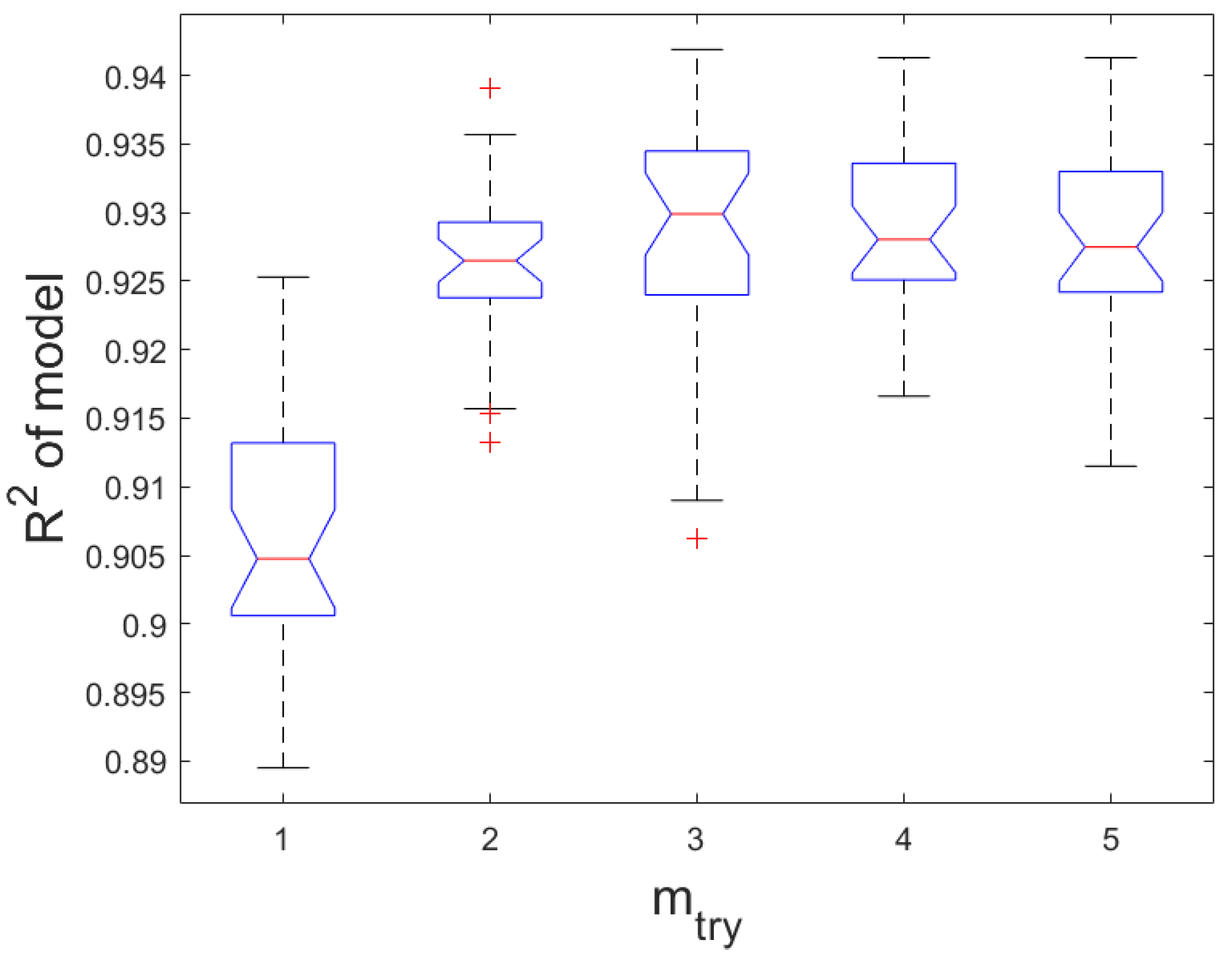
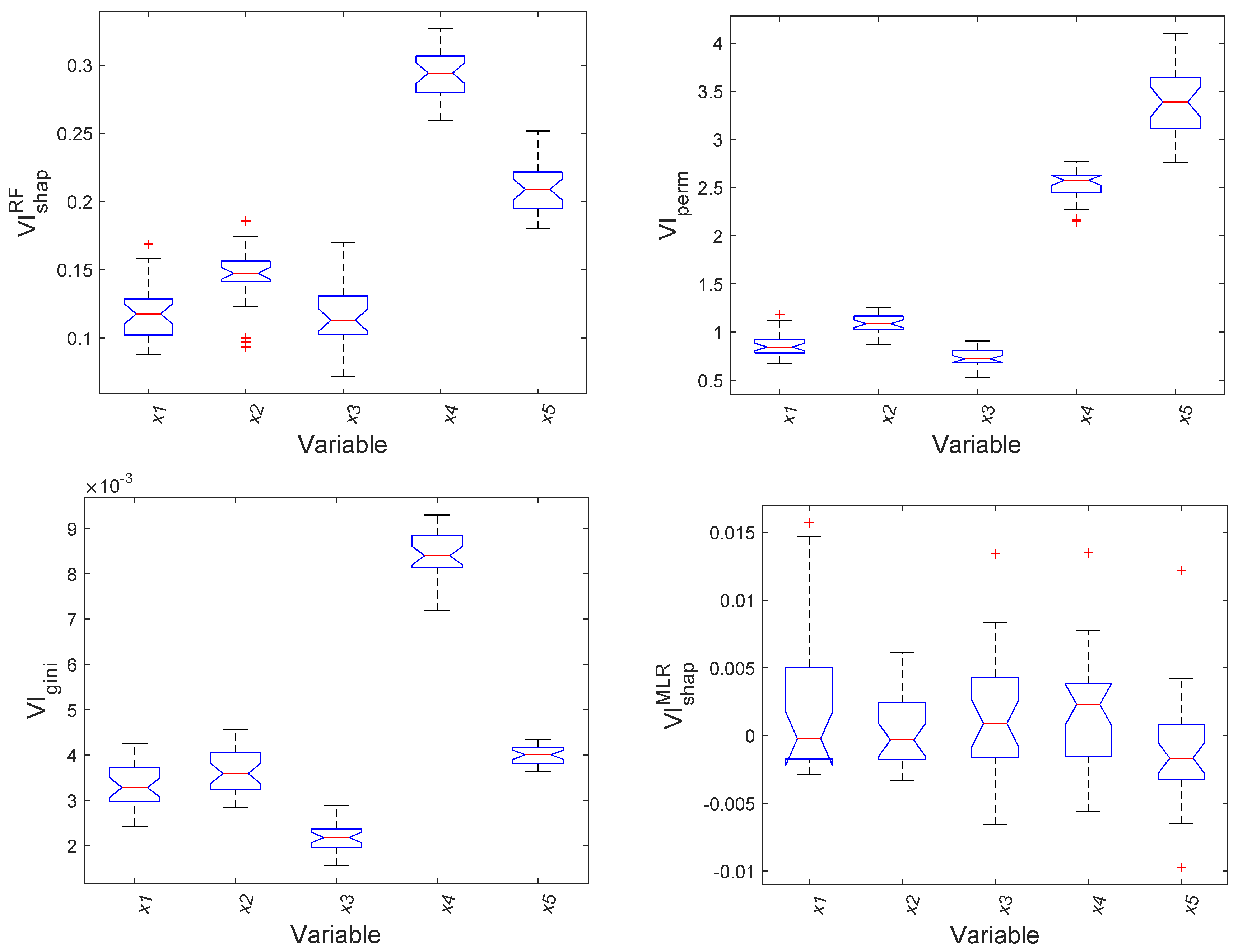
5.1. Linear System with Weakly Correlated Predictors

The data in the first case study were generated by the same model used by Olden et al. [29] to investigate variable importance analysis with multilayer perceptrons. A 1000 samples with six random variables were generated with a mean vector of zero and a covariance matrix ( Σ ) as follows.
Σ = | 1 0.2 0.2 0.2 0.2 0.8 0.2 1 0.2 0.2 0.2 0.6 0.2 0.2 1 0.2 0.2 0.4 0.2 0.2 0.2 1 0.2 0.2 0.2 0.2 0.2 0.2 1 0 0.8 0.6 0.4 0.2 0.2 1 |
The first five variables ( x 1 ,   x 2 , x 5 ) constituted the predictors, while the last variable ( y ,) was the target or response variable, linearly related to the predictor variables. The predictor variables were mildly correlated, as indicated by the covariance matrix in Equation (1), with bivariate correlation coefficients of r x i x j = 0.2 for all i , j . The first predictor variable ( x 1 ), was strongly correlated with the target variable, i.e., r x 1 y = 0.8 , the subsequent predictors having progressively weaker correlations, i.e., r x 2 y = 0.6 , r x 3 y = 0.4 , r x 4 y = 0.2 with the fifth predictor having no correlation with the target at all ( r x 5 y = 0 ).
Figure 2 shows a scatter plot matrix of the predictor data set (left), as well as the relationship between the response and the two most influential predictors.
Random forest models were fitted to the data, with the following optimal parameters: m t r y = 2 , n t r y = 80 % of the data, minimum leaf size, n l e a f = 5. On average, the random forest model could explain 93% of the variance of the response variable. The effect of the parameter m t r y on the performance of the model is shown in Figure 3
In addition to the random forest, multiple linear regression models were also run in a Shapley framework. The variable importance measures based on 30 runs are shown in Figure 4. These are the Shapley regression values (top, left), permutation indices (top, right), and Gini indices (bottom, left) obtained with random forest models, as well as the Shapley regression values obtained with a multiple linear regression model (bottom, right).
The boxes in the box plots show the median values of the importance measures (red horizontal bar in the center of the box), and the 25th and 75th percentiles (lower and upper edges of the boxes). The whiskers extend to the most extreme data points not considered outliers, which are indicated by ‘+’ markers. More specifically, points were drawn as outliers if they were larger than Q 3 + W ( Q 3 Q 1 ) or smaller than Q 1 W ( Q 3 Q 1 ) , where Q 1 and Q 3 are the 25th and 75th percentiles, respectively. W = 1.5 was used, corresponding to approximately 2.7 standard deviations of a normal distribution. The notches in the boxes can be used to compare the median values of the importance measures. That is, non-overlapping notches indicate a difference between the median values of the variables with 95% certainty.
The Shapley regression values obtained with the random forest are the only ones that could correctly identify the ranking of the importance of the variables, although the Gini importance measure came close to correct identification, as well. The Gini measure could rank variables x 1 to x 3 correctly, but the relative importance of variables x 4 and x 5 was swopped around by a small margin. The Shapley regression values obtained with the linear model yielded the same results as the Gini measure. Although significant, it is a relatively minor error again, bearing in mind that variable x 4 explains approximately 4% of the variance of the response only, as opposed to the zero percent of variable x 5 .
The permutation index could correctly identify the relative importance of variables x 4 and x 4 , but rated the relative importance of the fifth predictor as markedly higher than that of the fourth and also higher than that of the third predictor with 95% confidence. As discussed by Gregorutti et al. [30], the higher the interpredictor correlation and the larger the number of correlated predictors, the less important the predictor will appear to be, at least for additive models. On this basis, the variable importances of the last two variables would be fairly similar and would be difficult to distinguish from one another by any model. However, it does not explain the higher value of the last variable shown in Figure 4 (top, right).

5.2. Nonlinear System with Strongly Correlated Predictors

In the second case study, a simulated data set with 1000 samples was generated, where X 1000 × 5 and y 1000 × 1 , where y = x 4 2 + x 4 x 5 . The matrix X consisted of multivariate random numbers with a mean vector x ¯ = [ 0   0   0   0   0 ] and a covariance matrix Σ . As indicated by Equation (2), the first four ( x 1 , x 2 , x 3 , x 4 ) variables were strongly correlated with each other, while the last variable ( x 5 ) was independent from the other four.
The data are shown in Figure 5. As before, the random forest models were constructed with the same hyperparameters that were used in the first case study, except for m t r y = 4 . The effect of this parameter on the performance of the model is shown in Figure 6. On average, the random forest model could account for approximately 96% of the variance in the response variable, while the linear model was completely unable to capture the relationship.
Σ = | 1 0.9 0.9 0.9 0 0.9 1 0.9 0.9 0 0.9 0.9 1 0.9 0 0.9 0.9 0.9 1 0 0.9 0.9 0.9 1 0 0 0 0 0 1 |
The random forest Shapley variable importance indicator and the permutation index indicator were both able to identify the two important variables, x 4 and x 5 , although they differed in the ranking of these two variables. Interestingly, as indicated in Figure 7, the Gini variable importance measure could not distinguish the important variable x 5 from the unimportant variables x 1 , x 2 , and x 3 .
As expected, it is clear that a linear model could not give a reliable indication of the importance of the predictors.

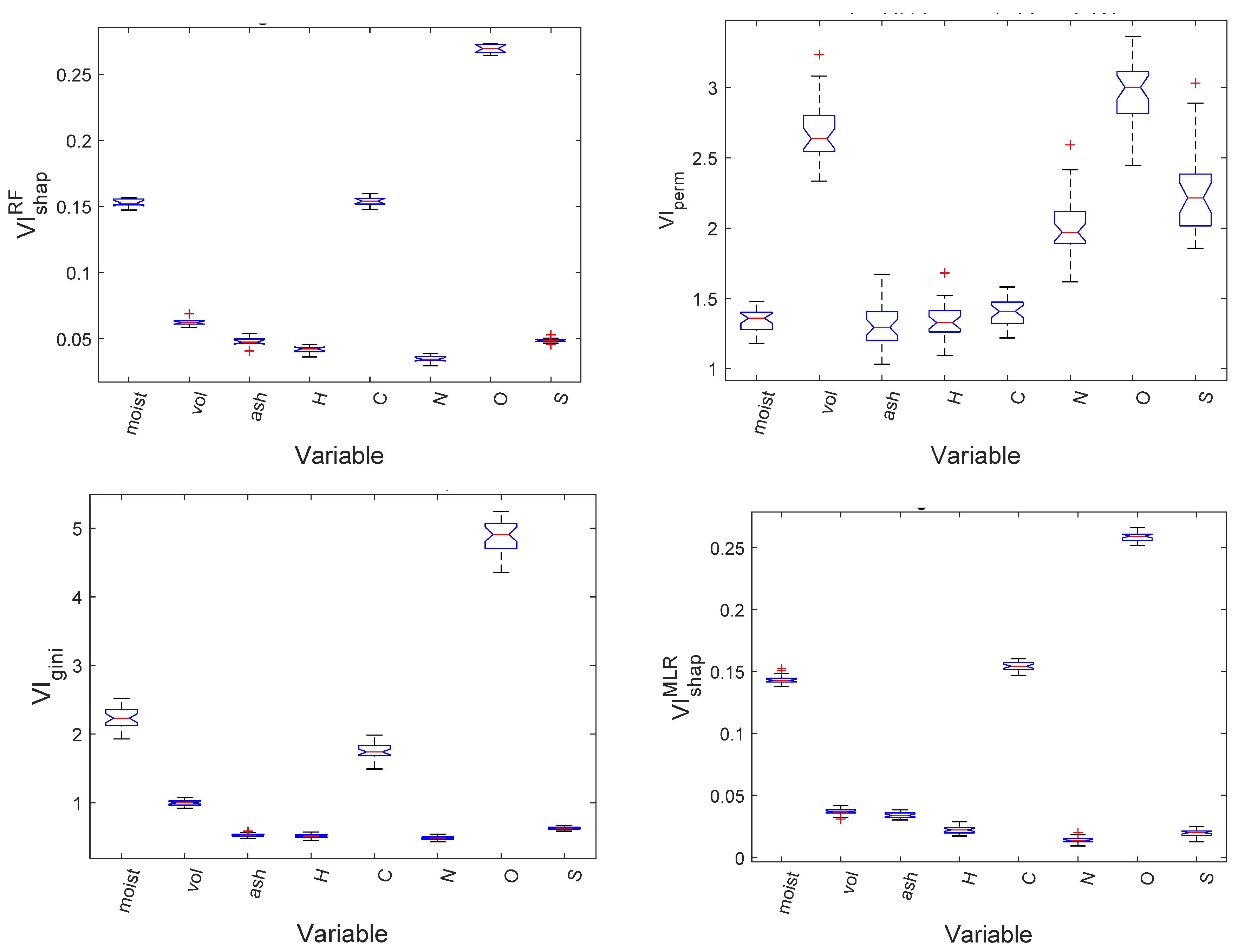
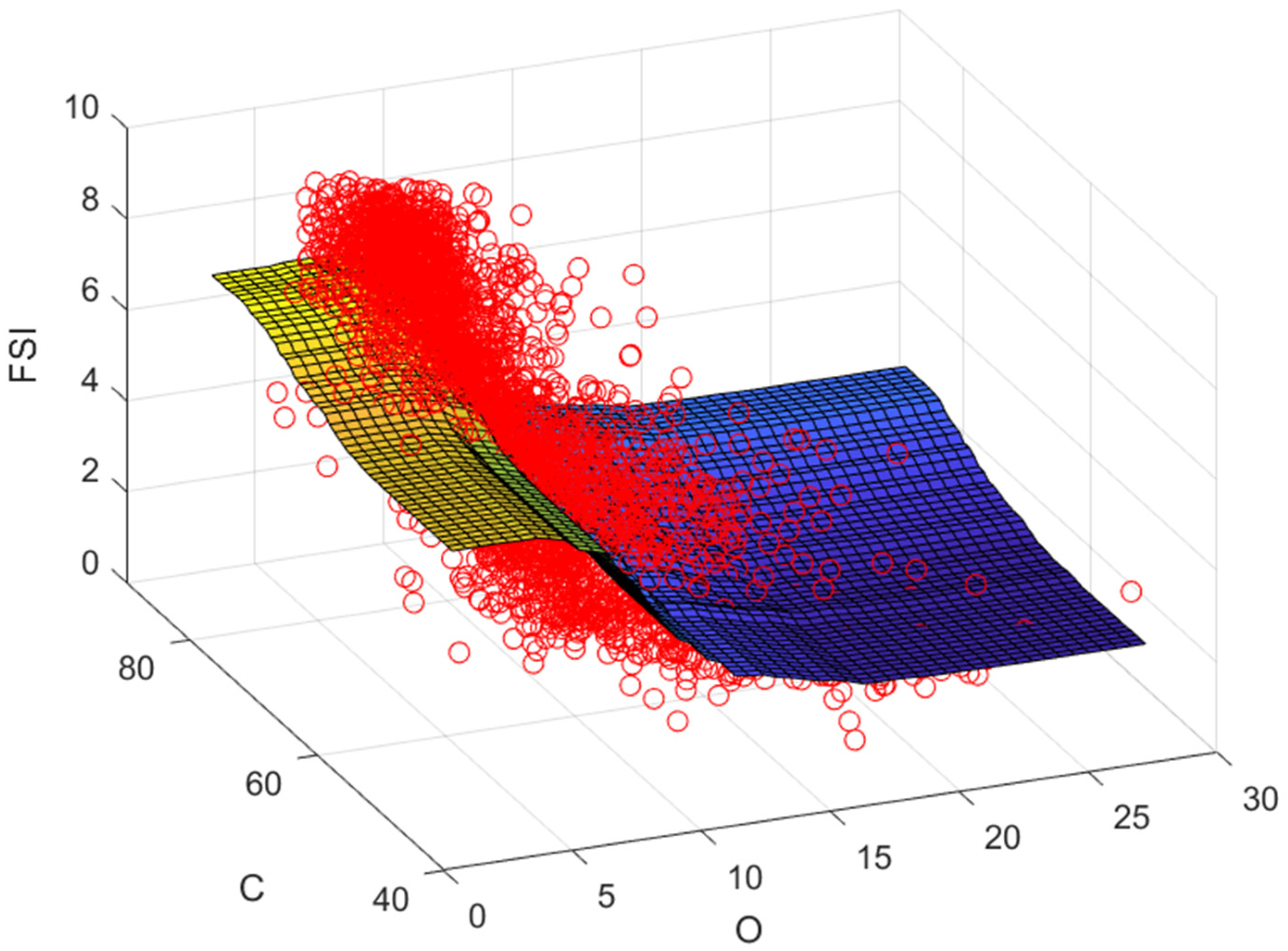
5.3. Free Swelling Index of Coal

Chelgani et al. [31] studied the free swelling index of coal. In this case study, the same data set is used, but only eight predictors variables ( x 1 ,   x 2 x 8 ) were considered, as indicated in Table 1. The predictor data matrix, X 3691 × 8 and the associated response vector, the free swelling index, y 3691 × 1 contained 3691 samples, which can be visualized based on a principal component score plot of the variables in Figure 8.
The 100-tree random forest model fitted to the data, with the following optimal hyperparameters: m t r y = 5 , n t r y = 80 % of the data, minimum leaf size, n l e a f = 5 was fitted to the data. This forest could explain approximately 82.5% of the variance of the free swelling index. The correlation coefficient matrix of the predictor data set is given in Table 2. From this table, it can be seen that variables x 1 , x 5 , and x 7 show significant correlation with the free swelling index (FSI).
With the full set of predictor variables, the random forest could explain approximately 82.7% of the variance of the free swelling index on average on unseen test data set. As indicated by the Shapley analysis, in Figure 9 (top, left), the three most important variables are the oxygen content ( x 7 ), carbon content ( x 5 ), and the moisture ( x 1 ) in the coal. The latter two variables are practically of equal importance.
Shapley analysis with a linear regression model gave markedly similar results (bottom, right, Figure 9), as did the random forest based on the Gini variable importance measure (bottom, left). However, except for the most important variable, the random forest model using the permutation importance index (top, right) yielded different results, suggesting, for example, that the nitrogen concentration ( x 6 ) is comparatively important, while this did not appear to be the case with the other models.
Figure 10 shows the partial dependence plots of the individual variables, as generated by the random forest model. Figure 11 shows the bivariate partial dependence plot of the two most important variables on the free swelling index of the coal, i.e., the oxygen and carbon content of the coal. The observed data are indicated by ‘o’ markers in this figure.

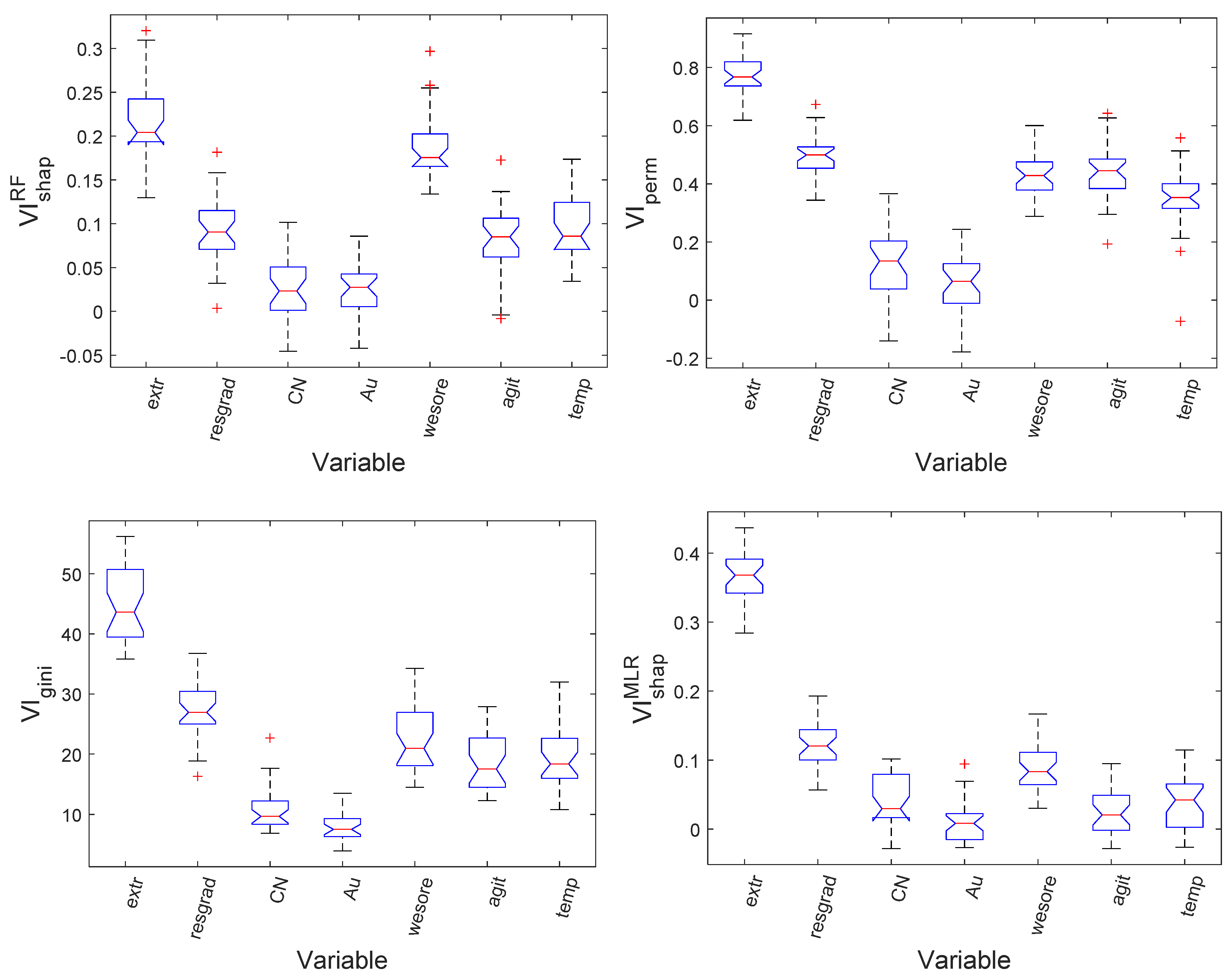
5.4. Consumption of Leaching Reagent in a Gold Circuit

In the final case study, a small data set related to the leaching of gold ore is considered, as described in Aldrich [32]. The consumption of lixiviant ( y ) depending on seven predictors variables ( x 1 ,   x 2 x 7 ) were considered. The variables represented the percentage extraction of the gold ( x 1 ), the residual grade of the ore ( x 2 ), the cyanide concentration in the leach tank ( x 3 ), the gold grade of the ore ( x 4 ), the source of the ore ( x 5 ), and the agitation rate of the tank ( x 6 ), as well as the leach temperature ( x 7 ).
The predictor data matrix, X 54 × 7 and the associated response vector, consumption of lixiviant, y 54 × 1 contained 54 samples. The correlation of the variables are summarized in Table 3. The 100-tree random forest model, with the following hyperparameters: m t r y = 4 , n t r y = 80 % of the data, minimum leaf size, n l e a f = 3 was fitted to the data. Figure 12 shows the decrease in the mean square error of the random forest model, as a function of the number of trees in the forest.
Figure 13 shows the results obtained with the different variable importance measures. The Shapley random forest variable importance measure identified variables x 1 and x 5 as significantly more important than the other variables.
Although the percentage extraction of the gold ( x 1 ) was identified as the most important variable by all the measures, as well, the results differ as far as the other variables are concerned. For example, the linear Shapley regression, permutation, and Gini variable importance indicators all flagged variable x 2 as the second most important variable. Figure 14 shows a bivariate partial dependence plot if the most important variables identified by the V I s h a p R F measure.

6. Discussion and Conclusions

In this paper, the use of random forest models in a Shapley regression framework was investigated, as a means to determine the importance of the predictors in these models. The results were compared with the widely used Gini and permutation importance measures used with random forests, as well as with multiple linear regression models, the latter also in the same framework.
Overall, the results suggest that the Shapley random forest variable importance measure yielded more reliable results than the other measures, at least with regard to the first two case studies based on simulated data.
The Gini importance measure is known to be biased towards variables with many categories or numeric values and even variables with many missing values [33]. However, in all the case studies considered here, the variables were of the same type, so this bias was not manifest. This may explain why the Gini importance measure arguably performed better than the permutation measure in two of the four case studies, and compared with mixed results in the other two case studies.
The random forest and multiple linear regression model used in a Shapley regression framework gave similarly reliable results for the linear system considered, as would be expected. However, the linear model broke down when it failed to capture the relationships in the nonlinear system in Case study 2, in particular.
Although the Shapley random forest measure arguably gave the most reliable results of the measures considered, these results would need to be validated by further work. Future work will also be extended to the use of other machine learning algorithms, such as multilayer perceptrons, which are also widely used as tools in variable importance analysis.

Funding

This research received no external funding.

Conflicts of Interest

The author declares no conflict of interest.

References

  1. Suriadi, S.; Leemans, S.J.J.; Carrasco, C.; Keeney, L.; Walters, P.; Burrage, K.; ter Hofstede, A.H.M.; Wynn, M.T. Isolating the impact of rock properties and operational settings on minerals processing performance: A data-driven approach. Miner. Eng. 2018, 122, 53–66. [Google Scholar] [CrossRef] [Green Version]
  2. Lipovetsky, S.; Conklin, M. Analysis of regression in game theory approach. Appl. Stoch. Models Bus. Ind. 2001, 17, 319–330. [Google Scholar] [CrossRef]
  3. Israeli, O. A Shapley-based decomposition of the R-Square of a linear regression. J. Econ. Inequal. 2007, 5, 199–212. [Google Scholar] [CrossRef]
  4. Grömping, U. Variable importance in regression models. Comput. Stat. 2015, 7, 137–152. [Google Scholar] [CrossRef]
  5. Budescu, D.V. Dominance analysis: A new approach to the problem of relative importance of predictors in multiple regression. Psychol. Bull. 1993, 114, 542–551. [Google Scholar] [CrossRef]
  6. Kruskal, W. Relative importance by analyzing over orderings. Am. Stat. 1987, 41, 6–10. [Google Scholar]
  7. Auret, L.; Aldrich, C. Interpretation of nonlinear relationships between process variables by use of random forests. Miner. Eng. 2012, 35, 27–42. [Google Scholar] [CrossRef]
  8. Aldrich, C. Consumption of steel grinding media in mills—A review. Miner. Eng. 2013, 49, 77–91. [Google Scholar] [CrossRef]
  9. Tohry, A.; Chelgani, S.C.; Matin, S.S.; Noorhammadi, M. Power-draw prediction by random forest based on operating parameters for an industrial ball mill. Adv. Powder Technol. 2019, 31, 967–972. [Google Scholar] [CrossRef]
  10. Bardinas, J.P.; Aldrich, C.; Napier, L.F.A. Predicting the operational states of grinding circuits by use of recurrence texture analysis of time series data. Processes 2018, 6, 17. [Google Scholar] [CrossRef] [Green Version]
  11. Shahbazi, B.; Chelgani, S.C.; Matin, S. Prediction of froth flotation responses based on various conditioning parameters by random forest method. Colloids Surf. A Physicochem. Eng. Asp. 2017, 529, 936–941. [Google Scholar] [CrossRef]
  12. Pu, Y.; Szmigiel, A.; Apel, D.B. Purities prediction in a manufacturing froth flotation plant: The deep learning techniques. Neural Comput. Appl. 2020, 2020, 1–11. [Google Scholar] [CrossRef]
  13. He, Z.; Tang, Z.; Yan, Z.; Liu, J. DTCWT-based zinc fast roughing working condition identification. Chin. J. Chem. Eng. 2018, 26, 1721–1726. [Google Scholar] [CrossRef]
  14. Nazari, S.; Chehreh Chelgani, S.Z.; Shafaei, B.; Shahbazi, S.S.; Matin, M. Gharabaghi, Flotation of coarse particles by hydrodynamic cavitation generated in the presence of conventional reagents. Sep. Purif. Technol. 2019, 220, 61–68. [Google Scholar] [CrossRef]
  15. Fu, Y.; Aldrich, C. Flotation froth image analysis by use of a dynamic feature extraction algorithm. IFAC-PapersOnLine 2016, 49, 84–89. [Google Scholar] [CrossRef]
  16. Aldrich, C.; Smith, L.K.; Verrelli, D.I.; Bruckard, W.J.; Kistner, M. Multivariate image analysis of a realgar-orpiment froth flotation system. Miner. Process. Extr. Metall. Trans. C. 2018, 127, 146–156. [Google Scholar]
  17. Tuşa, L.; Kern, M.; Khodadadzadeh, R.; Blannin, R.; Gloaguen, R.; Gutzmer, J. Evaluating the performance of hyperspectral short-wave infrared sensors for the pre-sorting of complex ores using machine learning methods. Miner. Eng. 2020, 146, 106150. [Google Scholar]
  18. Ohadi, B.; Sun, X.; Esmaieli, K.; Consens, S.P. Predicting blast-induced outcomes using random forest models of multi-year blasting data from an open pit mine. Bull. Eng. Geol. Environ. 2020, 79, 329–343. [Google Scholar] [CrossRef]
  19. Azen, R.; Budescu, D.V. The dominance analysis approach for comparing predictors in multiple regression. Psychol. Methods 2003, 8, 129–148. [Google Scholar] [CrossRef]
  20. Huettner, F.; Sunder, M. Axiomatic arguments for decomposing goodness of fit according to Shapley and Owen values. Electron. J. Stat. 2012, 6, 1239–1250. [Google Scholar] [CrossRef]
  21. Breiman, L. Random forests. Mach. Learn. 2001, 45, 5–32. [Google Scholar] [CrossRef] [Green Version]
  22. Strobl, C.; Malley, J.; Tutz, G. An introduction to recursive partitioning: Rationale, application, and characteristics of classification and regression trees, bagging, and random forests. Psychol. Methods 2009, 14, 323–348. [Google Scholar] [CrossRef] [PubMed] [Green Version]
  23. Carranza, E.J.M.; Laborte, A.G. Random forest predictive modelling of mineral prospectivity with small number of prospects and data with missing values in Abra (Philippines). Comput. Geosci. 2015, 74, 60–70. [Google Scholar] [CrossRef]
  24. Aldrich, C.; Auret, L. Fault detection and diagnosis with random forest feature extraction and variable importance methods. IFAC Proc. Vol. 2010, 43, 79–86. [Google Scholar] [CrossRef]
  25. Auret, L.; Aldrich, C. Unsupervised process fault diagnosis with random forests. Ind. Eng. Chem. Res. 2010, 49, 9184–9194. [Google Scholar] [CrossRef]
  26. Auret, L.; Aldrich, C. Change point detection in time series data with random forests. Control Eng. Pract. 2010, 18, 990–1002. [Google Scholar] [CrossRef]
  27. Auret, L.; Aldrich, C. Empirical comparison of tree ensemble variance importance measures. Chemom. Intell. Lab. Syst. 2011, 105, 157–170. [Google Scholar] [CrossRef]
  28. Archer, K.J.; Kimes, R.V. Empirical characterization of random forest variable importance measures. Comput. Stat. Data Anal. 2008, 52, 2249–2260. [Google Scholar] [CrossRef]
  29. Olden, J.D.; Joy, M.K.; Death, R.G. An accurate comparison of methods for quantifying variable importance in artificial neural networks using simulated data. Ecol. Model. 2004, 178, 389–397. [Google Scholar] [CrossRef]
  30. Gregorutti, B.; Michel, B.; Saint-Pierre, P. Correlation and variable importance in random forests. Stat. Comput. 2017, 27, 659–678. [Google Scholar] [CrossRef] [Green Version]
  31. Chelgani, C.S.; Matin, S.S.; Makaremi, S. Modelling of free swelling index based on variable importance measurement of parent coal properties by random forest methods. Measurement 2016, 94, 416–422. [Google Scholar] [CrossRef]
  32. Aldrich, C. Exploratory Analysis of Metallurgical Process Data with Neural Networks and Related Methods; Process Metallurgy Series 12; Elsevier Science B.V.: Amsterdam, The Netherlands, 2002; ISBN 0444503129. [Google Scholar]
  33. Strobl, C.; Boulesteix, A.-L.; Zeileis, A.; Hothorn, T. Bias in random forest variable importance measures: Illustrations, sources and a solution. BMC Bioinform. 2007, 8, 25. [Google Scholar] [CrossRef] [PubMed] [Green Version]
Figure 1. Diagrammatic representation of a random forest.
Minerals 10 00420 g001
Figure 2. Scatter plots of the predictor matrix X , showing bivariate relationships and the distributions of the variables x 1 ,   x 2 x 5 on the diagonal from top left to bottom right (left) and a 3D scatter plot of the simulated data set, y = f ( x 1 ,   x 2 ) (right).
Minerals 10 00420 g002
Figure 3. Effect of the random forest hyperparameter m t r y on the model performance in Case 1 based on 30 runs.
Minerals 10 00420 g003
Figure 4. Relative importance of predictors in Case Study 1, based on 100 iterations, showing Shapley values (top, left), permutation indices (top, right), Gini indices (bottom, left), and Shapley values for a multiple linear regression model (bottom, right), based on 30 runs.
Minerals 10 00420 g004
Figure 5. Scatter plots of the predictor matrix X , showing bivariate relationships and the distributions of the variables x 1 ,   x 2 x 5 on the diagonal from top left to bottom right (left) and 3D scatter plot of the simulated data set, y = x 4 2 + x 4 x 5 (right).
Minerals 10 00420 g005
Figure 6. Effect of the random forest hyperparameter m t r y on the model performance in Case 2 based on 30 runs.
Minerals 10 00420 g006
Figure 7. Variable importance analysis with the Shapley regression forest (top, left), permutation with the random forest (top, right), Gini index with the random forest (bottom, left), and Shapley regression with a linear model (bottom, right), based on 30 runs.
Minerals 10 00420 g007
Figure 8. Principal component score plot of the eight predictor variables in the free swelling index system (left) and a scatterplot of the most important variables (right). The colors imposed on the markers show the corresponding values of the free swelling index, as indicated by the color bar.
Minerals 10 00420 g008
Figure 9. Variable importance analysis with the Shapley regression forest (top, left), permutation random forest (top, right), Gini random forest (bottom, left), and Shapley linear regression (bottom, right), based on 30 runs.
Minerals 10 00420 g009
Figure 10. Partial dependence plots for predictors of the free swelling index of coal.
Minerals 10 00420 g010
Figure 11. Bivariate partial dependence plot showing the effect of the two most influential predictors on the free swelling index of coal. The observed data are indicated by ‘o’ markers.
Minerals 10 00420 g011
Figure 12. Decrease in mean square error (MSE) with number of trees in the random forest model of the leach system based on 100 runs.
Minerals 10 00420 g012
Figure 13. Variable importance analysis with the Shapley regression forest (top, left), permutation random forest (top, right), Gini random forest (bottom, left), and Shapley linear regression (bottom, right), based on 30 runs.
Minerals 10 00420 g013
Figure 14. Bivariate partial dependence plot showing the effect of the two most influential variables, x 1 and x 5 , on reagent consumption. The observed data are indicated by ‘o’ markers.
Minerals 10 00420 g014
Table 1. Predictor variables in coal data set.
x 1 x 2 x 3 x 4 x 5 x 6 x 7 x 8
MoistureVolAshHCNOS
Table 2. Correlation coefficient matrix of the predictors and response variable in the coal data set.
x 1 x 2 x 3 x 4 x 5 x 6 x 7 x 8 y
x 1 1.0000.024−0.0500.397−0.594−0.3250.9190.086−0.597
x 2 0.0241.000−0.2410.482−0.0580.0680.1660.343−0.258
x 3 −0.050−0.2411.000−0.693−0.711−0.364−0.1100.370−0.091
x 4 0.3970.482−0.6931.0000.2200.1840.425−0.176−0.185
x 5 −0.594−0.058−0.7110.2201.0000.491−0.569−0.4980.570
x 6 −0.3250.068−0.3640.1840.4911.000−0.281−0.3360.160
x 7 0.9190.166−0.1100.425−0.569−0.2811.000−0.046−0.748
x 8 0.0860.3430.370−0.176−0.498−0.336−0.0461.000−0.042
y −0.597−0.258−0.091−0.1850.5700.160−0.748−0.0421.000
Table 3. Correlation coefficient matrix of the predictors and response variable in the leach data set.
Variables x 1 x 2 x 3 x 4 x 5 x 6 x 7 y
x 1 10.644−0.3960.173−0.2800.004900.4170.678
x 2 0.6441−0.305−0.113−0.2690.04550.2000.502
x 3 −0.396−0.3051−0.2140.2660.4680.167−0.294
x 4 0.173−0.113−0.2141−0.0512−0.1850.1500.156
x 5 −0.280−0.2690.266−0.05121−0.0247−0.4430.169
x 6 0.004900.04550.468−0.185−0.024710.392−0.229
x 7 0.4170.2000.1670.150−0.4430.3921−0.0212
y 0.6780.502−0.2940.1560.169−0.229−0.02121

