An Interpretable Extreme Gradient Boosting Model to Predict Ash Fusion Temperatures


Abstract
1. Introduction
2. Materials and Methods
2.1. Data Set
- Ash chemical composition (content of the following oxides: SiO2, Al2O3, Fe2O3, CaO, MgO, Na2O, K2O, SO3, TiO2, P2O5 and Mn3O4) according to standard ISO 13605:2018,
- Hemispherical temperature of ash (HT) in a reducing atmosphere (mixture of CO:CO2 in a ratio of 3:2) according to standard PN-ISO 540:2001.
2.2. Extreme Gradient Boosting (XGBoost)
- yi—real value,
- —the prediction at the r-th round,
- gr—term denoting structure of decision tree,
- —loss function,
- n—number of training examples,
- —regularization term, given by formula:
- T—number of leaves,
- ω—weight of the leaves,
- λ and γ are coefficients, with default values set as λ = 1, γ = 0.
2.3. Feature Importance (FI)
2.4. Partial Dependence Plots (PDP)
- S—chosen predictor,
- C—the complement set of S (containing all other predictors),
- —feature vectors,
- —marginal probability density of .
- —the values of that occur in the training sample.
2.5. Model Evaluation
- Mean absolute error (MAE):
- Root mean squared error (RMSE):
- Coefficient of determination R2:
- yi—the actual value of the dependent variable,
- di—the value of the dependent variable determined from the model,
- —the arithmetic mean of the actual values of the dependent variable.
2.6. Software
3. Results and Discussion
3.1. Feature Importance
3.2. Determining the Optimal Values of Model Hyperparameters
- n_estimators = 200—refers to number of trees in the ensemble,
- learning_rate = 0.08—step size shrinkage used in update to prevents overfitting,
- gamma = 0.3—minimum loss reduction required to make a further partition on a leaf node of the tree,
- subsample = 0.95—controls the number of samples (observations) supplied to a tree,
- min_child_weight = 1.5—the minimum number of instances required in a child node,
- colsample_bytree = 0.8—controls the number of features (variables) supplied to a tree,
- max_depth = 8—controls the depth of the tree.
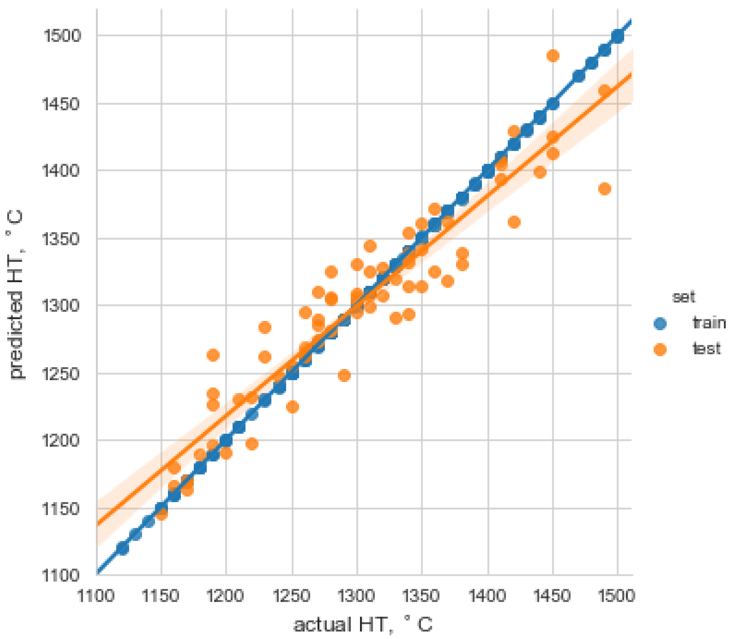
3.3. Evaluation of the Model
- mean absolute error: 21.71,
- Root mean squared error: 29.16,
- R2: 0.88.
- Support vector regression (SVR) with RBF (radial basis function) kernel function, hyperparameters of that model were determined with grid search procedure: C = 1, ε = 0.01, γ = 10,
- Multiple linear regression (MLR), the coefficients of the model were determined by the least mean square algorithm.
3.4. Model Interpretation Using PDPs (Partial Dependence Plots)
4. Conclusions
- The aim of this study was to create a HT prediction model. The machine learning method was used for this purpose—XGBoost regressor, well known to provide better solutions than other machine learning algorithms.
- The effect of 11 different ash components (oxides) on HT prediction was investigated using the feature importance technique. The results showed that Al2O3 had the most significant influence on HT prediction, then respectively, Fe2O3, SO3, Na2O and CaO.
- The partial dependence plots technique was used to examine whether the relationship between the particular oxide and a predicted HT was linear, monotonic or more complex. It was revealed that:
- ○
- HT of coals increased, as the content of Al2O3 in the ash became higher. However, a significant increase of fusibility was observed when the Al2O3 content in the ash was higher than about 25%.
- ○
- The ash fusion temperature decreased as the concentration of Na2O in the ash increased. However, this trend was reversed when the Na2O content exceeded 3%. An amount of Na2O in ash higher than about 5% no longer contributed to changes in HT.
- ○
- As the Fe2O3 content increased, HT of coal samples decreased. However, when the concentration of Fe2O3 exceeded about 13%, the changes of HT were not significant.
- ○
- It can be seen that HT of the coal decreased with the increase of the CaO content until reaching the minimum around 12% content of CaO. Then fusibility increased gradually with the increase of the CaO content.
- ○
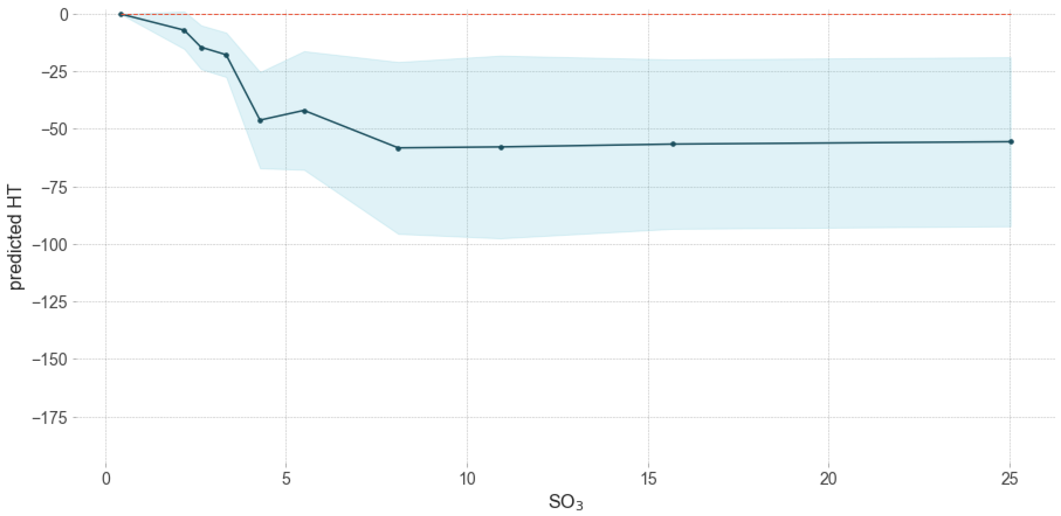
- HT of coals decreased, as the content of SO3 became higher. A significant reduction of HT was observed when the content of SO3 was in range of 0–5%. Meanwhile the concentration of SO3 exceeded about 10%, the changes of HT were not significant. However, it should be indicated that SO3 did not exist in isolation in coal ash minerals, but together with other elements (Ca, Mg) in the sulfate form. Therefore, the cations in the chemical compounds had an effect on slag chemistry, not SO3 itself.
- ○
- SiO2 fraction did not significantly affect the predicted HT.
- Results showed that the model created in this study could predict the HT with satisfactory efficiency R2 equal to 0.88. Finally, the results proved that XGBoost could be used as a reliable method for predicting HT.
Author Contributions
Funding
Conflicts of Interest
References
- Liu, B.; He, Q.; Jiang, Z.; Xu, R.; Hu, B. Relationship between coal ash composition and ash fusion temperatures. Fuel 2013, 105, 293–300. [Google Scholar] [CrossRef]
- Vassileva, G.C.; Vassilev, S.V. Relations between Ash-Fusion Temperatures and Chemical and Mineral Composition of Some Bulgarian Coals. Comptes Rendus l’Academie Bulg. Sci. 2002, 55, 6–61. [Google Scholar]
- Sharma, A.; Saikia, A.; Khare, P.; Dutta, D.K.; Baruah, B.P. The chemical composition of tertiary Indian coal ash and its combustion behaviour—A statistical approach: Part 2. J. Earth Syst. Sci. 2014, 123, 1439–1449. [Google Scholar] [CrossRef]
- Vassilev, S.V.; Kitano, K.; Takeda, S.; Tsurue, T. Influence of mineral and chemical composition of coal ashes on their fusibility. Fuel Process. Technol. 1995, 45, 27–51. [Google Scholar] [CrossRef]
- Van Dyk, J.C.; Keyser, M.J.; Van Zyl, J.W. Suitability of feedstocks for the Sasol–Lurgi fixed bed dry bottom gasification process. In Proceedings of the Gasification Technologies Conference, San Francisco, CA, USA, 7–10 October 2001. [Google Scholar]
- Seggiani, M. Empirical correlations of the ash fusion temperatures and temperature of critical viscosity for coal and biomass ashes. Fuel 1999, 78, 1121–1125. [Google Scholar] [CrossRef]
- Gray, V.R. Prediction of ash fusion temperature from ash composition for some New Zealand coals. Fuel 1987, 66, 1230–1239. [Google Scholar] [CrossRef]
- Jak, E. Prediction of coal ash fusion temperatures with the F*A*C*T thermodynamic computer package. Fuel 2002, 81, 1655–1668. [Google Scholar] [CrossRef]
- Luxsanayotin, A.; Pipatmanomai, S.; Bhattacharya, S. Effect of mineral oxides on slag formation tendency of Mae Moh lignites. Songklanakarin J. Sci. Technol. 2010, 32, 403–412. [Google Scholar]
- Li, F.; Yu, B.; Wang, G.; Fan, H.; Wang, T.; Guo, M.; Fang, Y. Investigation on improve ash fusion temperature (AFT) of low-AFT coal by biomass addition. Fuel Process. Technol. 2019, 191, 11–19. [Google Scholar] [CrossRef]
- Yazdani, S.; Hadavandi, E.; Chelgani, S.C. Rule-Based Intelligent System for Variable Importance Measurement and Prediction of Ash Fusion Indexes. Energy Fuels 2017, 32, 329–335. [Google Scholar] [CrossRef]
- Goni, C.; Helle, S.; Garcia, X.; Gordon, A.; Parra, R.; Kelm, U.; Jimenez, R.; Alfaro, G. Coal blend combustion: Fusibility ranking from mineral matter composition. Fuel 2003, 82, 2087–2095. [Google Scholar] [CrossRef]
- Carpenter, A. Coal Blending for Power Stations; IEA Coal Research: London, UK, 1995. [Google Scholar]
- Huggins, F.E.; Kosmack, D.A.; Huffman, G.P. Correlation between ash-fusion temperatures and ternary equilibrium phase diagrams. Fuel 1981, 60, 577–584. [Google Scholar] [CrossRef]
- Lloyd, W.G.; Riley, J.T.; Zhou, S.; Risen, M.A.; Tibbitts, R.L. Ash fusion temperatures under oxidizing conditions. Energy Fuels 1993, 7, 490–494. [Google Scholar] [CrossRef]
- Lolja, S.A.; Haxhi, H.; Dhimitri, R.; Drushku, S.; Malja, A. Correlation between ash fusion temperatures and chemical composition in Albanian coal ashes. Fuel 2002, 81, 2257–2261. [Google Scholar] [CrossRef]
- Özbayoğlu, G.; Özbayoğlu, M.E. A new approach for the prediction of ash fusion temperatures: A case study using Turkish Lignites. Fuel 2006, 85, 545–562. [Google Scholar] [CrossRef]
- Shi, W.J.; Kong, L.X.; Bai, J.; Xu, J.; Li, W.C.; Bai, Z.Q.; Li, W. Effect of CaO/Fe2O3 on fusion behaviors of coal ash at high temperatures. Fuel Process. Technol. 2018, 181, 18–24. [Google Scholar] [CrossRef]
- Winegartner, E.C.; Rhodes, B.T. An empirical study of the relation of chemical properties to ash fusion temperatures. J. Eng. Power 1975, 97, 395–403. [Google Scholar] [CrossRef]
- Gao, F.; Han, P.; Zhai, Y.J.; Chen, L.X. Application of support vector machine and ant colony algorithm in optimization of coal ash fusion temperature. In Proceedings of the 2011 International Conference on Machine Learning and Cybernetics, Guilin, China, 10–13 July 2011; IEEE: Piscataway, NJ, USA, 2011. [Google Scholar] [CrossRef]
- Karimi, S.; Jorjani, E.; Chelgani, S.C.; Mesroghli, S. Multivariable regression and adaptive neurofuzzy inference system predictions of ash fusion temperatures using ash chemical composition of us coals. J. Fuels 2014, 2014, 1–11. [Google Scholar] [CrossRef]
- Miao, S.; Jiang, Q.; Zhou, H.; Shi, J.; Cao, Z. Modelling and prediction of coal ash fusion temperature based on BP neural network. In MATEC Web of Conferences Volume 40 (2016), Proceedings of the 2015 International Conference on Mechanical Engineering and Electrical Systems (ICMES 2015), Singapore, 16–18 December 2015; Chang, G.A., Ma, M., Arumuga Perumal, S., Chen, G., Eds.; EDP Sciences: Les Ulis, France, 2016; pp. 5–10. [Google Scholar]
- Sasi, T.; Mighani, M.; Örs, E.; Tawani, R.; Gräbner, M. Prediction of ash fusion behavior from coal ash composition for entrained-flow gasification. Fuel Process. Technol. 2018, 176, 64–75. [Google Scholar] [CrossRef]
- Seggiani, M.; Pannocchia, G. Prediction of coal ash thermal properties using partial least-squares regression. Ind. Eng. Chem. Res. 2003, 42, 4919–4926. [Google Scholar] [CrossRef]
- Tambe, S.S.; Naniwadekar, M.; Tiwary, S.; Mukherjee, A.; Das, T.B. Prediction of coal ash fusion temperatures using computational intelligence based models. Int. J. Coal Sci. Technol. 2018, 5, 486–507. [Google Scholar] [CrossRef]
- Xiao, H.; Chen, Y.; Dou, C.; Ru, Y.; Cai, L.; Zhang, C.; Kang, Z.; Sun, B. Prediction of ash-deformation temperature based on grey-wolf algorithm and support-vector machine. Fuel 2019, 241, 304–310. [Google Scholar] [CrossRef]
- Yin, C.; Luo, Z.; Ni, M.; Cen, K. Predicting coal ash fusion temperature with a back-propagation neural network model. Fuel 1998, 77, 1777–1782. [Google Scholar] [CrossRef]
- Zhao, B.; Zhang, Z.; Wu, X. Prediction of coal ash fusion temperature by least squares support vector machine model. Energy Fuels 2010, 24, 3066–3071. [Google Scholar] [CrossRef]
- Żogała, A.; Rzychoń, M.; Łączny, M.J.; Róg, L. Selection of optimal coal blends in terms of ash fusion temperatures using Support Vector Machine (SVM) classifier—A case study for Polish coals. Physicochem. Probl. Miner. Process. 2019, 55, 1311–1322. [Google Scholar] [CrossRef]
- Mielecki, T. Studies on Coal Examination and Properties (In Polish); Silesia Publishing House: Katowice, Poland, 1971. [Google Scholar]
- Chen, T.; Guestrin, C. Xgboost: A scalable tree boosting system. In Proceedings of the 22nd ACM SIGKDD International Conference on Knowledge Discovery and Data Mining, San Francisco, CA, USA, 13–17 August 2016; Krishnapuram, B., Ed.; ACM: New York, NY, USA, 2016; pp. 785–794. [Google Scholar] [CrossRef]
- Machine Learning Wins The Higgs Challenge. Available online: http://cds.cern.ch/journal/CERNBulletin/2014/49/News%20Articles/1972036 (accessed on 8 January 2020).
- Friedman, J.H. Greedy function approximation: A gradient boosting machine. Ann. Stat. 2001, 29, 1189–1232. Available online: https://www.jstor.org/stable/2699986 (accessed on 8 January 2020). [CrossRef]
- Basu, S.; Debnath, A.K. Power Plant Instrumentation and Control Handbook: A Guide to Thermal Power Plants, 1st ed.; Academic Press: Cambridge, MA, USA, 2014. [Google Scholar] [CrossRef]
- Tomeczek, J.; Palugniok, H. Kinetics of mineral matter transformation during coal combustion. Fuel 2002, 81, 1251–1258. [Google Scholar] [CrossRef]
- Szuflicki, M.; Malon, A.; Tymiński, M. The Balance of Mineral Resources Deposits in Poland (In Polish); Polish Geological Institute—National Research Institute: Warsaw, Poland, 2019. [Google Scholar]
- Marsland, S. Machine Learning: An Algorithmic Perspective, 2nd ed.; Taylor & Francis Inc.: Milton Park, UK, 2014. [Google Scholar]
- Natekin, A.; Knoll, A. Gradient Boosting Machines, A Tutorial. Front. Neurorobot. 2013, 7, 21. [Google Scholar] [CrossRef]
- Hastie, T.; Tibshirani, R.; Friedman, J. The Elements of Statistical Learning, Data Mining, Inference and Prediction, 2nd ed.; Springer Science & Business Media: New York, NY, USA, 2009. [Google Scholar]
- Breiman, L.; Friedman, J.; Olshen, R.; Stone, C. Classification and Regression Trees; Wadsworth Inc.: Belmont, TN, USA, 1984. [Google Scholar]
- Molnar, C. Interpretable Machine Learning, A Guide for Making Black Box Models Explainable; Version Dated, 10; Munich, Germany, 2018; ISBN 9780244768522. Available online: https://christophm.github.io/interpretable-ml-book/ (accessed on 18 January 2020).
- Vorres, K.S. Melting behavior of coal ash materials from coal ash composition. Div. Fuel Chem. 1977, 22, 118. [Google Scholar]
- Liu, C.; Bai, Y.; Yan, L.; Zuo, Y.; Wang, Y.; Li, F. Impact of alkaline oxide on coal ash fusion temperature. Int. J. Oil Gas Coal Technol. 2014, 8, 79. [Google Scholar] [CrossRef]


| Standard:ISO PN-ISO 540:2001 | Description |
|---|---|
| Initial deformation temperature (IDT) | The temperature at which the first change of form of the sample occurs (rounding of the corners or apex). |
| Spherical temperature (ST) | The temperature at which the cone fuses down to a spherical lump at which the height is equal to the width of the base. |
| Hemispherical temperature (HT) | The temperature at which the cone fuses down to a hemispherical lump at which point the height is one half the width of the base. |
| Fluid temperature (FT) | The temperature at which the fused mass of sample spreads out in a nearly flat layer. |
| Parameter | Mean | Standard Deviation | Min | Max |
|---|---|---|---|---|
| HT, °C | 1310.6 | 82.95 | 1120.0 | 1500.0 |
| SiO2, % | 40.09 | 13.0 | 8.71 | 63.88 |
| Al2O3, % | 22.17 | 5.1 | 7.66 | 35.06 |
| Fe2O3, % | 11.09 | 4.77 | 2.99 | 35.49 |
| CaO, % | 7.86 | 5.13 | 0.79 | 25.14 |
| MgO, % | 4.43 | 2.56 | 0.72 | 14.0 |
| Na2O, % | 2.4 | 1.63 | 0.24 | 8.79 |
| K2O, % | 1.86 | 0.94 | 0.15 | 9.09 |
| SO3, % | 7.17 | 5.42 | 0.42 | 25.02 |
| TiO2, % | 0.92 | 0.29 | 0.07 | 2.66 |
| P2O5, % | 0.75 | 0.77 | 0.04 | 5.1 |
| Mn3O4, % | 0.15 | 0.07 | 0.02 | 0.67 |
| Model | R2 |
|---|---|
| MLR | 0.34 |
| SVR | 0.83 |
| XGBoost | 0.88 |
© 2020 by the authors. Licensee MDPI, Basel, Switzerland. This article is an open access article distributed under the terms and conditions of the Creative Commons Attribution (CC BY) license (http://creativecommons.org/licenses/by/4.0/).
Share and Cite
Rzychoń, M.; Żogała, A.; Róg, L. An Interpretable Extreme Gradient Boosting Model to Predict Ash Fusion Temperatures. Minerals 2020, 10, 487. https://doi.org/10.3390/min10060487
Rzychoń M, Żogała A, Róg L. An Interpretable Extreme Gradient Boosting Model to Predict Ash Fusion Temperatures. Minerals. 2020; 10(6):487. https://doi.org/10.3390/min10060487
Chicago/Turabian StyleRzychoń, Maciej, Alina Żogała, and Leokadia Róg. 2020. "An Interpretable Extreme Gradient Boosting Model to Predict Ash Fusion Temperatures" Minerals 10, no. 6: 487. https://doi.org/10.3390/min10060487
APA StyleRzychoń, M., Żogała, A., & Róg, L. (2020). An Interpretable Extreme Gradient Boosting Model to Predict Ash Fusion Temperatures. Minerals, 10(6), 487. https://doi.org/10.3390/min10060487