Predicting the Spatial Distributions of Elements in Former Military Operation Area Using Linear and Nonlinear Methods Across the Stavnja Valley, Bosnia and Herzegovina ^†

Abstract

This study has the purpose of developing a realistic soil prediction maps of the spatial distribution of elements by evaluating and comparing different modelling techniques: Kriging, artificial neural network-multilayer perceptron (ANN-MLP) and multiple polynomial regressions (MPR). The Stavnja Valley was selected as a test area due to the following reasons: (1) intensive metal ore mining and metallurgical processing; (2) peculiar geomorphological natural features; (3) regular geological setting, and (4) the remaining minefields. Geospatial parameters from digital elevation models (DEM) are used as an input to advanced prediction modelling techniques: ANN-MLP and MPR. Soil measurements, land use data, and remote sensing are applied, developed, and finally incorporated into the models of spatial distribution in the form of 2D or 3D maps. In order to reconstruct the different processes that influenced the entire study area simultaneously, we used novel approaches to modelling. This comprehensive approach not only represents an innovation in contamination mapping, but developed prediction models also help in the reconstruction of main distribution pathways, assess the real size of the affected area, and improve the data interpretation.

1. Introduction

The dynamic equilibrium between erosion, transport, and deposition that occurs in most natural river systems [1], can be interrupted by human activities. Many worldwide rivers are significantly affected by multiple metals contaminants due to past and present mining activities, [2]. Metal containing particles are quite often transported over large distances by water affecting the alluvial sediments, even several hundred kilometres away from the main sources of contamination [3,4,5,6]. Metal ore mining and processing lead to some of the largest releases of trace elements causing a considerable impact on the surrounding environment. Obsolete metal production technologies used for mass production generated an enormous quantity of mining waste which is considered hazardous due to the presence of toxic metals [7,8]. Important sources of trace elements in the metal industry include different stages, starting from mining and milling operations, concentrating, ore transporting, disposal of tailings, wastewater, followed by the smelting process that includes concentrating, sintering, atmospheric discharges, and blowing dust [9]. It is known that many ore minerals accommodate various other trace metals as minor inclusions, causing contamination with major and minor ore metals in the areas surrounding mines and smelters [10,11,12].

The environmental concern in mining areas is primarily related to physical disturbance of the surrounding landscape, mine tailings spill, emitted dust and acid mine drainage (AMD) transported into rivers. The adverse effects of mining and smelting activities in the environment have been addressed by many authors in many parts of the world [13,14,15,16,17,18,19,20].

Great potential for improvement of predictive soil mapping (PSM) techniques and understanding of the relationships between soils and the environment has been created after the increase in computer efficiency and capacity, geo-information technology, data availability, and demand accurate and reliable maps [21,22,23,24].

This requires the creation of spatial soil information based on numerical models, which account for the spatial and temporal variations in soil properties based on soil information and related environmental variables [25].

The Stavnja river valley has been known for intensive mining and metallurgical activities for more than 100 years. Besides these activities, the valley has been selected for the study due to several other reasons such as (1) unique geological setting, especially the metallogenic belt, (2) the geomorphological characteristics that affect the contamination halo, and (3) remaining minefields from the last war, 1992–1995. The anthropogenic impact in the municipality of Vareš can be reflected through the three abandoned iron ore deposits (Smreka, Brezik, and Droškovec), abandoned Pb–Zn–Ba deposit Veovača and abandoned ironwork Vareš, and brown coal mining in the southern part of the study area. High concentrations of particular elements are released into the environment not only by anthropogenic activities but also by natural erosion and weathering reactions of parental rocks that add to the complexity of the environmental assessment [26]. Problems of contamination along the river can be demonstrated as anisotropic appearance between the layered (isotropic) lithological units, which can be solved using advanced linear and nonlinear modelling techniques instead of denser sampling grid which is restricted by the remaining minefields at 5%–6% of the study area.

The multivariate techniques such as linear and nonlinear are widely used in geology. For example, mapping soil organic matter, mapping presence/absence elements or mapping physical property of model, asses hazard and contaminated area [27,28]. The main purpose of this study was to develop a visualization model of spatial distribution using linear and nonlinear mathematical methods that combine a sparse chemical analysis and various geospatial parameters in Stavnja Valley (Bosnia and Herzegovina) but in the same time to evaluate and compare the performance of different modelling techniques: Kriging, artificial neural network—multilayer perceptron (ANN-MLP), and multiple polynomial regressions (MPR). For this reason, five specific purposes of the present study were: (1) to include various geospatial parameters in linear and nonlinear modelling; (2) to identify main distribution pathways and change in concentrations according to the distance from the source of contamination; (3) model verification; (4) to assess the real size of the affected area; and (5) to provide an optimal methodology for geochemical researchers in areas with restricted sampling conditions.

2. Material and Methods

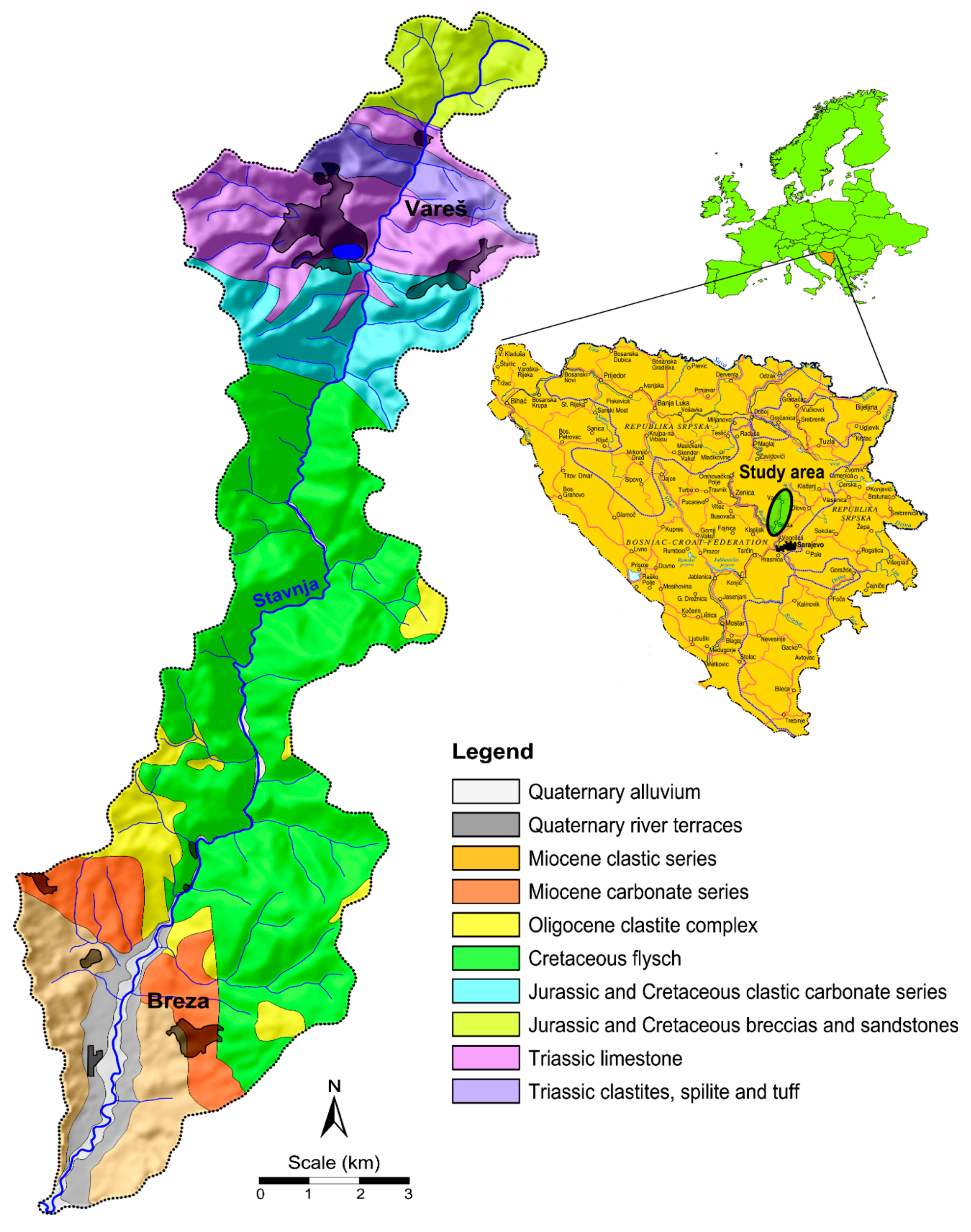
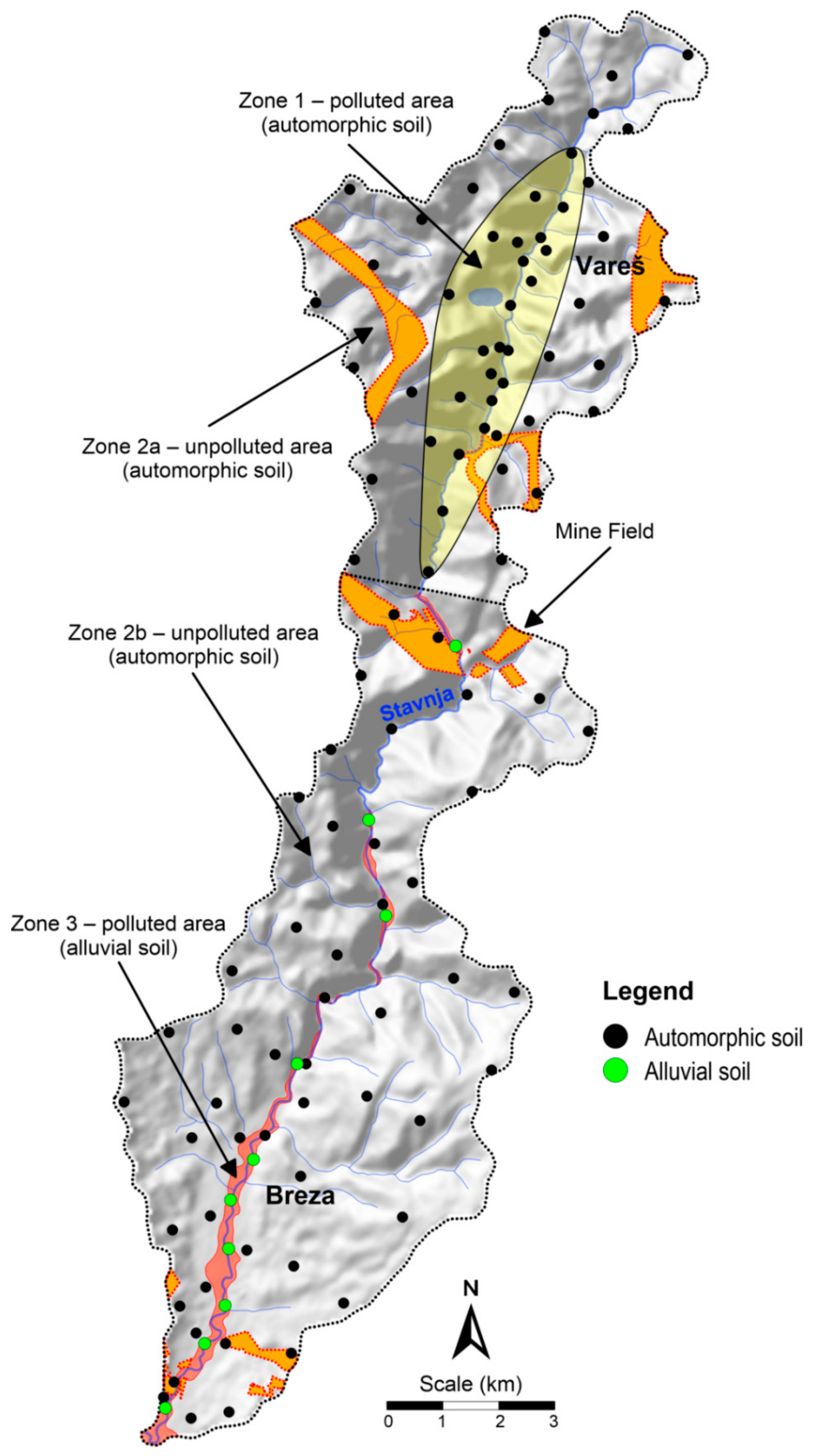
2.1. Description of the Study Area

The physiography of the region displays a high variety. Contrasting landscapes are found from the mountain environment in the northern part of the study, more than 1000 m altitudes and in the southern part about 400 m. The river Stavnja has a length of about 35 km, located in Central Bosnia and Herzegovina, northern from the capital Sarajevo (Figure 1). Approximately 30,000 inhabitants live in this Valley, mostly settled into two small cities Vareš and Breza. The study site has been the place of military operation during the last war (1992–1995). In the valley, three ethnic groups, namely Orthodox, Catholics, and Bosniaks, lived close to each other, which resulted in massive conflict, destruction, killing, and burning. According to the available maps, between 5 and 6 km² of the study area is covered by the minefields.

The valley is known for intensive mining and metallurgical activities for more than 100 years. In the municipality of Vareš, three abandoned iron ore deposits (Smreka, Brezik, and Droškovec) are located, in which estimated reserves and resources were approximately 170 million tonnes in 1991. Apart from the iron deposits, Eastern from the city Vareš, the multi-element (Lead-Zinc-Barite) open pit Veovača is located. Southern from the urban zone sits the ironworks Vareš, which construction began in 1889, after Austrian-Hungarians arrivals to Bosnia and Herzegovina. A city Breza with surrounding settlements developed in the South of the study area that is known as brown coal mining (open pits and underground). This coal basin belongs to the Central Bosnian coal basin that lies along the river Bosna.

The outcropping stratigraphic sequence exposes rock formations spanning from the Palaeozoic ages embedded into Upper Triassic to more recent times. Ten major lithological units are present in the study (Figure 1). The river Stavnja perpendicularly crosses the lithological units, from the oldest ones in the north to the youngest in the south. Younger Quaternary layers are developed along a present watercourse or something higher in gravel-conglomerate terraces [29]. The study area is a part of the Durmitor nappe. The most important geotectonic unit of Vareš metallogenic district belongs to the Central ophiolite zone. Vareš, siderite–hematite sedimentary exhalative (SEDEX) deposits at Smreka, Droškovac, and Brezik are locus typicus mineralization of the Mid-Triassic. The deposits contain hydrothermal, stratiform siderite–hematite–chert beds. The mineralization forms part of the Anisian and Ladinian sequences and displays distinct vertical zoning, reflecting a gradual change of redox conditions in the depositional environment. The sequence starts with bituminous, thinly bedded shales with pyrite and base metal sulphides, overlain by barite and siderite, deposited under reducing conditions. Overlying clastics and oolithic limestone are succeeded by hematite shale, hematite ± chert beds, deposited in an oxidizing environment. Major minerals are siderite, manganese-rich hematite, barite, pyrite, marcasite, chalcopyrite, galena, sphalerite, tetrahedrite, and Pb-sulphosalts. Veovača Pb, Zn, Ba deposit contains ore-breccia or ore conglomerates with dm- to m-sized clasts cemented by barite and Pb–Zn sulphides. Microcrystalline dark barite is accompanied with galena and sphalerite. The barite from Veovača is typical for Triassic SEDEX deposits elsewhere in the Dinarides [30].

2.2. Sampling Design, Sample Preparation, and Analytical Methods

According to the primary purpose of research, previous sampling experience [18,19,26,31,32,33,34] and facing other difficulties and challenges (such as the narrow gorge, inaccessible terrain, and minefields) any regular sampling grid couldn’t be used. Considering all the above-mentioned, the sampling grid had been designed to cover the entire Valley with a sampling grid in order to determine: a change in altitude, distance from the main sources of pollution, a transport mode (atmospheric or river transport), and shape of the contamination halo areole. In the urban and industrialized areas, the sampling grid is denser (Figure 2). At the same time, the sampling grid has been created so that all main lithological units are covered with a significant number of samples which is necessary for the determination of bedrock influence. Each sampling site is recorded by the central point position with a GPS device. Whereas the reliability of the mine maps is relatively low (perhaps between 70–80%), we put special emphasis on integration and communication with local people who lived there before and after the war.

At places of intensive military operations, many minefields still remain, especially parts of strategic importance such as roads, industrial objects, bridges, etc. According to our experience, before sampling important following steps should be considered: (1) to learn as much as possible about the sampling site (political situation, ethnic groups); (2) to have a map with remaining minefields and possible minefields; (3) to talk to the local people, and (4) be aware of any object that looks like a mine, such as the wire or small tins, etc. According to our experience, such sampling should be done in a group of two or three people maximum, if possible, with one local. The distance between two people should be about 40 m, in case that one activates the mine, another can help. One route should be used in both directions: to the sampling site and on the way back. If possible, existing routes or hard surfaces should be used for walking.

The following sampling sites shouldn’t be selected for sampling: near burned houses; near the strategic objects; near bridges which were often used as a border between two military sides/conflict groups; sampling in bushes, high grass, and forests. In the case of soil, sampling is safer to choose the meadows and pastures because they are used for livestock grazing (cows, sheep, goats, etc.). During the digging of soil profiles, everyone should be aware that unexploded mine can be activated. Sampling in such areas is very risky because a spade is stabbed into the depth of 30 cm where it should be kept in mind that one sampling site is composed of a minimum of five subsamples that increase the risk. Similar advice can be applied for the stream sediment sampling. Here is a problem that some unexploded projectiles can be transported far from the minefields and can be embedded in deeper layers.

In 2014, Bosnia and Herzegovina suffered tremendously from flood, and in many cases the landmines were dislodged. Dislodging is not affecting only Bosnian people but can create an international problem if floodwaters carry the explosives downstream through southeast Europe. Even the stabilization force (SFOR) several years after the war organized anonymous action for collecting any kind of weapons, but unfortunately, some people decided to cast off, dig, or hide them in surrounding rivers, forests, etc.

Soils are the most widespread sampling material used for their environmental assessment due to their availability and relatively undemanding sampling method. High variability of soil chemistry can be dispatched by taking composite samples. In this study, one soil sample represents the composite material collected at the central sample point itself at five points within a radius of 50 m around it. At each sampling point, topsoil (0–5 cm) and subsoil (20–30 cm) are collected and the mass of such a composite was about 1 kg [26,32]. According to the sampling sites, the collected soils can be genetically divided into two main groups, the automorphic soil, and alluvial soil, respectively. The automorphic soils [35] belong to the Cambisol, type of soil developed on meadow and pastures. Soils developed on the youngest Quaternary material (alluvium) are called fluvisol (FAO classification).

To begin with, the soil samples (n = 222) were air-dried and later completely dried in a fan drier at 40 °C. The dry material was disaggregated in a ceramic mortar and sieved through a 2 mm nylon screen and pulverized to a fine powder [34]. All samples were analysed at the ACME, Ltd. laboratory in Vancouver, Canada [36]. Determination of 36 chemical elements (Ag, Al, As, Au, B, Ba, Bi, Ca, Cd, Co, Cr, Cu, Fe, Ga, Hg, K, La, Mg, Mn, Mo, Na, Ni, P, Pb, S, Sb, Sc, Se, Sr, Th, Ti, Tl, U, V, W, and Zn) was performed by ICP-MS after aqua regia digestion (mixture HCl, HNO₃ and water at 95 °C).

3. Techniques used in Modelling

3.1. Data Processing

For this purpose various spatial data were acquired by digitalization of existing topographic maps (provided by the Geodetic Survey of Bosnia and Herzegovina), Google Earth maps [37], geological maps (provided by Geological Survey of Slovenia and Geological Survey Federation of Bosnia and Herzegovina) and SRTM 90 m digital elevation data (DEM) [38]. Because the topographic maps were amended in the late 1970s, they were combined with the Google Earth maps. The isolation of major lithological units is also an important step for the determination of natural and anthropogenic background. Digitalization, vectorization, additional modification, standardization of databases and integration to GIS environment were performed using Surfer 11 (Golden Software) and QGIS (GNU General Public Licence).

A database includes the following information: (1) the basic descriptive parameters such as the Identification number, Sample label, Sampling material, (2) analytical data (concentrations of elements); and (3) geospatial data such as landuse unit, lithological unit, defined zones, latitude, longitude, absolute distance from the ironworks chimneys, elliptical distance from the ironworks chimneys, distance from the river Stavnja, altitude, altitude above the bottom of Stavnja valley, terrain slope, aspect, plan curvature, profile curvature, tangent curvature, Landsat spectral bands 1–7. For the spatial distribution modelling of particular elements using artificial neural network and multiple polynomial regression, a system of grid cells has been used. For this purpose, the whole study area is divided into a 50 × 50 m grid cell. The total number of grid cells is 41.471, which has been described by the aforementioned attributive parameters [26].

3.2. Data Transformation

Transforming data means performing the same mathematical operation on each piece of original data which the main purpose is to reduce the difference between extreme values [39]. It is often observed that environmental variables are Log-normal [40,41,42] or positively skewed [43,44] and data transformation is necessary to normalize such data sets. The Box-Cox transformation represents one of the most frequently used transformations in environmental sciences and geosciences where power transformation is needed [45,46,47,48,49].

The Box-Cox transformation is given by:

$$y= \frac{X^{\lambda }-1}{\lambda };\hspace{1em}\lambda \ne 0$$

where y is the transformed value and x is the value to be transformed. The $\lambda$ coefficient varies from −5 to 5. All values of λ are considered and the optimal value is the one which results in the best approximation of a normal distribution curve.

3.3. Kriging

Kriging is a term that covers a range of methods used to describe spatial optimal linear prediction with minimum errors. The method most used is ordinary kriging. It estimates the value at a region for which a variogram is known, using data in the neighbourhood. The semivariance function used in ordinary kriging is based on the assumption that nearby objects tend to be more similar than those that are farther apart.

The accuracy of values estimated with kriging lies in the fact that every estimated point comes with its estimation variance. Additionally, the spatial structure of the parameters is being observed. The geostatistical method of kriging is widely applied in the mapping of soil attributes in unsampled areas [50]. At the same time, this enables quantification of the main spatial characteristic of soil attributes and spatial interpolation methods considering only the neighbouring points of estimation data [51,52].

The first step of kriging is calculating an unbiased estimator of the semivariance function that is half of the average squared difference between paired data values:

$$y \left(h\right)= \frac{1}{2N \left(h\right)} {\displaystyle \sum }_{i=1}^{N\left(h\right)}{\left[Z\left(x_i\right)-Z\left(x_i+h\right) \right]}^2$$

where γ(h) is the semivariance at a given distance h; and N(h) is the number of sample pairs in h, and z(x_i + h) and z(x_i) are sample values at two points separated by h.

The semivariogram model is combined with various theoretical models like Gaussian, exponential, spherical, linear and power by the weighted least square method. The spatial variability of the data set and the resulting grid file are also mathematically specified. The interpolation weights, which are applied to the data points during the grid node calculations, are direct functions of the variogram model [53]. Graphical displaying is a final goal of many environmental scientists in the chain of steps that begins with sampling which prime objective is to utilize the power of visual appearance [54].

In this paper, the application of kriging to the spatial distribution of elements has been shown.

3.4. Artificial nNeural Network—Multilayer Perceptron

Artificial neural networks (ANN) have received considerable attention over recent years with a wide range of applications, accordingly in soil science research. The method is suitable for dealing with nosy data and modelling the non-linear behaviour of data. The term neural network is inspired by the biological nervous systems. It is composed of many highly interconnected processing elements (neurons or nodes) working synchronously to solve specific problems. An ANN is configured for a specific application, such as pattern recognition or data classification, through a learning process. Learning in biological systems involves adjustments to the synaptic connections that exist between the neurons [55]. The synapses transmit signals to the other neurons which then process it and also signal the neurons nearby.

Rosenblatt [56] with his perceptron, as the first model for learning with a teacher, laid the foundation for the development of a layered feed-forward ANN. Rosenblatt’s algorithm is referred to as a single-layer perceptron. The ANN uses a multilayer perceptron (MLP) which is identified by its architecture, that performs tasks such as function fitting and pattern recognition problems [57]. The learning logarithm as a part of MLP is used for the backpropagation of error, i.e., resilient propagation variation. MLPs are feedforward neural networks (FNNs) with one or more layers of units between the input and output layers [58,59,60].

The output of a neuron is given by:

$$\xi ={\displaystyle \sum }_{i=1}^n{w}_i{x}_i-b=w^{T}x-b$$

$$y=\sigma \left(\xi \right)$$

where $x_i$ is the ith input, w_i is the link weight from the ith input, w = (w_i... w_n)^T, x = (x₁... x_n)^T, b is a threshold or bias, and $n$ is the number of inputs. The activation function $\sigma \left(\xi \right)$ is usually some continuous or discontinuous function mapping the real numbers into the interval (−1,1) or (0,1) [56]. A different function can be used as an activation function but the most used is the sigmoidal activation function. The standard sigmoidal activation function has the following form:

$$\sigma \left(\xi \right)= \frac{1}{1 + e^{-\xi }}$$

The success of the method can be laid down for the following reasons: (1) They can model extremely complex systems and due to their nature can be used to model nonlinear natural systems (linearity in the sense of mathematical properties of additivity and homogeneity); when using linear algebra (such as most of the multivariate statistics) to describe nonlinear systems we always have to make an approximations; (2) There is no limitation with the dimensionality of the problem; it can be arbitrary, depending on the CPU speed and memory; and (3) simple and successful operation due to well-developed learning algorithms [61].

3.5. Multiple Polynomial Regressions

Multiple regression the term was first used by Pearson 1908 [62], refers to regression application which is designed to handle multiple inputs; predictions are made with a single dependent variable and multiple independent variables. Polynomial regression is a type of multiple regression analysis used when the variables show a curvilinear trend. It is modelled as an mth order polynomial [63]. The general polynomial regression model is given by:

$$Y_i={\beta }_{0 }+{\beta }_{1 }x+ {\beta }_{2 } x^2+ {\beta }_{3 } x^3+\dots + {\beta }_{m } x^m+ {\epsilon }_i$$

where, for a set of I observations, Y_i is the dependent variable, β₀ is a regression constant, β₁,β₂,…,β_m are the coefficients of the X, X²,…, X^m independent variables (predictors), m is order of the polynomial, and Ɛ_I is the model error (the difference between observations and predicted values).

Although polynomial regression fits a nonlinear model to the data, the estimation problem is linear because the regression coefficients are linear in the parameters [64]. The regression analysis aims at establishing the values of the parameters of the regression equation and to find the best fit and quantify it with respect to the dependent variable (Y) [59]. Two values, R² and adjusted R², describe how well the model fits the data. All regression models provide information based on the influence of the combined interactions of the estimator variables on the response. However, the major conceptual limitation of the regression techniques is that one can only ascertain relationships, but never be sure about the underlying causal mechanism.

4. Results and Discussion

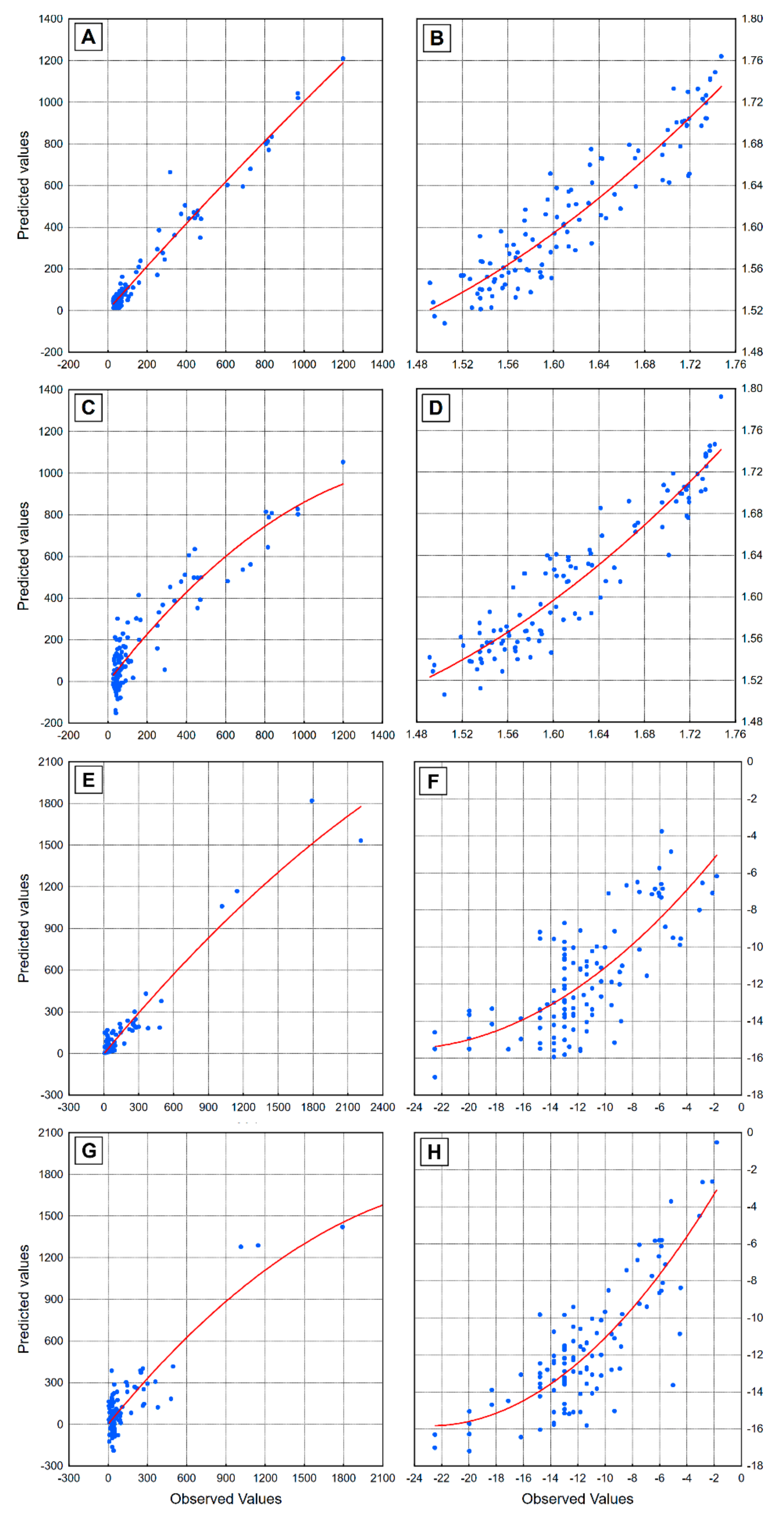
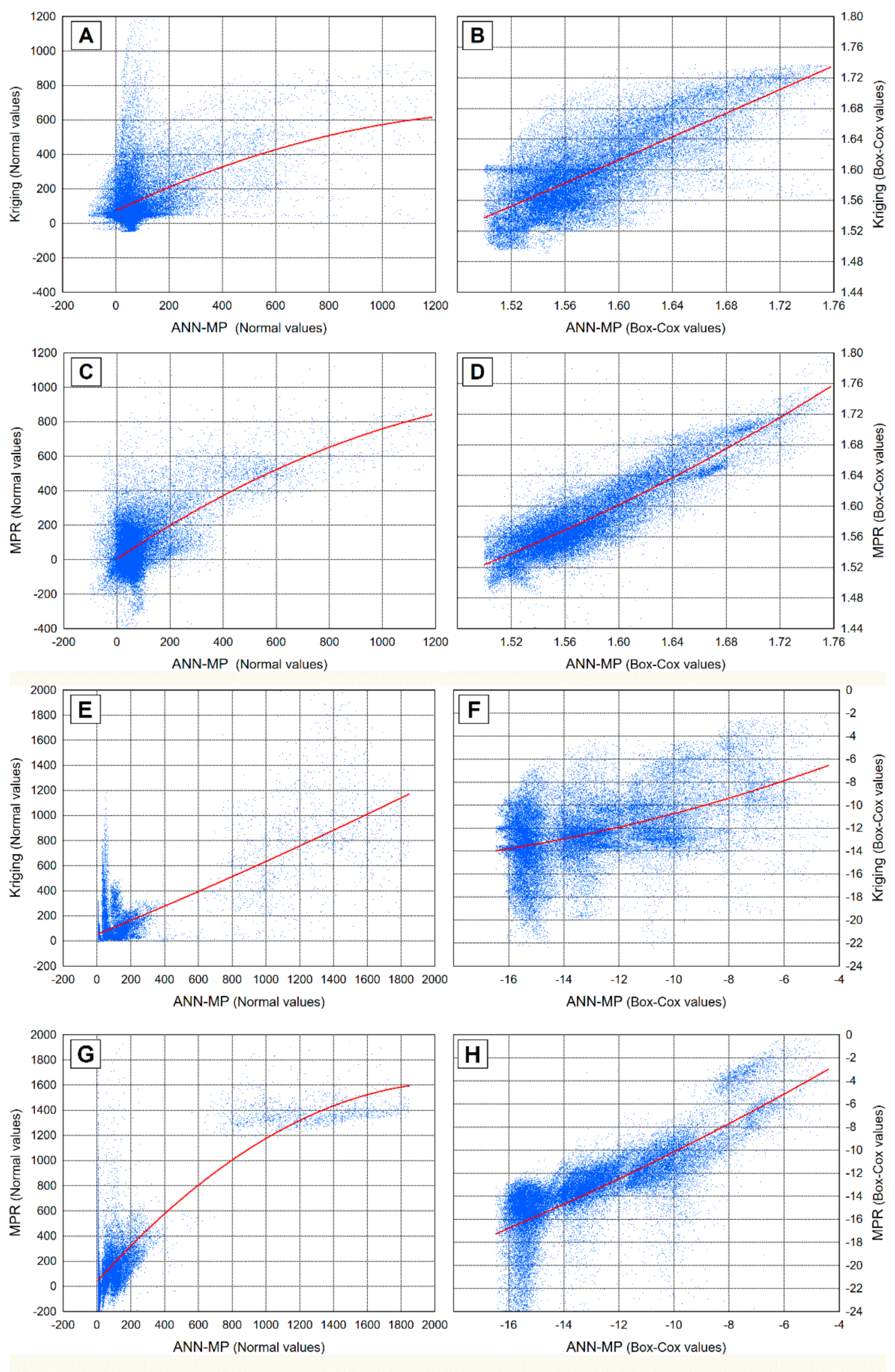
4.1. Linear Method (MPR) vs. Nonlinear Method (ANN-MLP)

Due to the high cost and time-consuming nature of soil sampling, research in developing methods for the creation of soil maps from sparse soil data is becoming increasingly important. In recent years, the development of prediction methods (linear and nonlinear) that use secondary attributes sourced from the DEM, land use, and remote sensing in combination with sparse and expensive soil measurements has sharpened the focus of the research. Various modelling techniques applied for soil prediction were compared, and the best combination of prediction method and secondary information was chosen. Various modelling techniques help us reconstruct different processes that influenced the entire study area. Simultaneously, they distinguish natural and anthropogenic influences as well as transportation patterns (such as atmospheric or water transport). Their main purpose is not only to isolate the hotspots with the highest concentrations but also to provide a spatial distribution pattern of particular trace elements.

All aforementioned geospatial data were used in two prediction methods, multiple polynomial regression (MPR) and artificial neural network-multilayer perceptron (ANN-MLP), respectively. For both modelling methods, a recall grid was used. Both methods were treated by the same conditions and same software packages, Statistica 11 [65] and Surfer 11 [66]. Modelling by ANN-MLP was done by using a large number of input data, 240 hidden units and 25 training networks. Changes in some input data, a number of neurons, as well as the number of training networks was performed in order to obtain the best models. More neurons and more architecture will acquire better results. Each particular model is trained to 25 networks but only five logical networks were retained, and finally, an average model of five retained networks was calculated. Each training model contains a summary table with following parameters: training perfection, test perfection, validation perfection, all perfection, training error, test error, validation error, training algorithm, hidden activation, and output activation. Modelling by MPR is much more difficult than ANN-MLP. To get a useful model, so many data conversion, corrections, and transformations have to be performed and one must be chosen for the best optimization algorithm [67]. The MPR is a very demanding method, comparing to the ANN-MLP, and much more input data is needed. This method is developed as a controlling method. Their main goal is confirmation of its success, certainty, and superiority over the other methods.

The use of various geospatial parameters is developed over recent years and its use is necessary for the development of the prediction method. But there are two problems that must be considered when ANN-MLP is applied: (1) The use of secondary attributes and calculated parameters in some cases could imply at subjectivity in data processing; (2) Much subjectivity can lead to inappropriate data interpretation due to the fact that the learning process is overloaded. When referring to overloading, it doesn’t mean that the numbers of input data are large, but that the final results can only follow one particular parameter such as the slope, aspect, distance from the source of contamination, etc. In such cases, the spatial distributions are completely useless and cannot be considered in data interpretation. Sometimes it is necessary to repeat the whole process of learning or in some extreme cases to remove the parameter from further analysis.

4.2. Model Stability and Model Signification

The essence of the whole approach is to create stable and repeatable results under the same conditions. Procedures, approaches, data preparation, and calculations have been developed so long until the spatial distributions that represents the geochemical characteristics of the landscape for both methods become stable, repeatable and realistic. The estimation of model applicability and reliability of prediction lies in the fact that all created models are repeatable. This means that the developed procedures are not random or specific to a particular item or an isolated area, but such a model can be used without a limitation. The method has been critically evaluated according to the significance of the applied transformations, the similarity between models, as well as the stability of predictions. Simultaneously, the MPR method was developed in order to prove the results of artificial intelligence and its superiority. However, the results obtained by linear methods are extremely useful and our theory about the superiority of the nonlinear method was wrong. Comparing the performances of these two different machine learning algorithms, it is distinguished that ANN-MP already provides highly reliable results with a small number of input data, whereas the MPR is a very demanding method requiring more mathematical knowledge and geospatial data.

The regression has been performed for both prediction methods before data transformation (raw data) and after Box-Cox transformation. Model stability and model signification have been tested on the distribution of Pb which represents a dominant anthropogenic pattern in the chosen study area and Ti that represents a natural distribution, mainly related to the one particular lithological unit.

Table 1. Comparison between the statistical parameters of raw data (n = 111) and predicted values (n = 41,471).

Element	Transformation	X¯	Md	A	E	X2	KS
Pb (N)	Raw values	190	62	2.66 *	8.13 *	139.2 *	0.32 *
Pb (B)	Box-Cox	72	62	0.37 NS	−0.20 NS	28.7 NS	0.11 NS
Ti (N)	Raw values	130	35	5.02 *	28.02 *	109.4 *	0.34 *
Ti (B)	Box-Cox	42	35	−0.11 NS	0.50 NS	16.6 NS	0.12 NS

X¯—mean; Md—median; A—skewness; E—kurtosis; X²—Chi-Square test; KS—Kolmogorov-Smirnov test; NS—no significance; *—significance at p < 0.05; N—raw values; B—Box-Cox.

presents some basic statistical parameters between normal and transformed data for the two selected elements (Pb a Ti) that represent the two most common patterns in the study area, within the raw data and predicted data. It can be observed that the work with raw data doesn’t bring predicted results and compositional data in such studies must be transformed. Suitability of using the Box-Cox transformation is reflected in the fact that the distributions of natural values are significantly asymmetric. The negative values for Pb and Ti already appear up to 25 percentiles. Also, the mean and median values are higher than predicted values, but in the case of Pb, it could be explained by the fact that the sampling grid had been denser in areas with dominant human impact. The prediction assurance is measured by the cubic polynomial regression between the predicted and observed values. It should be clear that this measurement has been performed only on ANN-MP and MPR because they depend on (geo) spatial parameters. Contrary to these two modelling techniques, the Kriging method is affected by changes in concentration and distance between the observations. In order to test the normality with skewness, kurtosis, Kolmogorov–Smirnov test, and Chi-Square test between raw data and Box-Cox transformation have been performed.

The model quality for MPR is described with the following coefficients: R (correlation between the observed values and predicted values), Multiple R² (coefficient of determination), and Adjusted R² (adjusted coefficient of determination) (

Table 2. Model quality of MPR and ANN-MP.

MPR
Element	Multiple R	Multiple R2	Adjusted R2	F Ratio
Pb (N)	0.93	0.86	0.81	16.9
Pb (B)	0.94	0.87	0.83	18.6
Ti (N)	0.78	0.60	0.45	4.0
Ti (B)	0.90	0.82	0.75	11.8
ANN-MP
Element	Training Perfection	Test Perfection	Validation Perfection	All Perfection
Pb (N)	0.93	0.91	0.94	0.92
Pb (B)	0.99	0.98	0.89	0.98
Ti (N)	0.79	0.87	0.73	0.80
Ti (B)	0.96	0.87	0.95	0.94

). Those parameters determine how well the model fits the data. It can be observed that the difference between raw data and transformed data for Pb is very low, which is conditioned by several extremely high concentrations. For Ti, this difference is higher. The penalize tendency of increasing the R squared when additional predictors are included in the model, the R2-adjusted is used. The ANN-MP model quality is described with different parameters than MPR. Training perfection, test perfection, validation perfection, all perfection is high for both selected elements after the data transformation.

Regressions between transformations within the two predictive methods are provided in scatterplots with fitted regression lines in Figure 3. It is evident that Pb distribution (A–D) is tending to show exponential form, but this is affected by several samples with very high levels. The scatterplots for both predictive methods, ANN-MP and MPR (A and C) are showing quite similar tendencies, representing a result of the strong asymmetric distribution. It is typical for anthropogenic elements, where extreme levels deviate from the low levels of parental rocks. Differences between untransformed and transformed data (Box-Cox) are almost negligible for both modelling techniques (B and D). The data are transformed by applying a single mathematical function to all the raw data values, leading to symmetric distribution, stabilizing variance, and making the distribution closer to normal.

Similar results are obtained for the model stability evaluation for Ti (Figure 3E–H). The correlation diagrams for raw data are showing that there is practically no real effective connection between observed and predicted values for both advanced modelling techniques (E and G). After applying the Box-Cox transformation is achieved a significant improvement in both methods (F and H). This can be explained by the fact that geochemical and pedological data arrive in several batches at different levels and a systematic relationship between spread and level is often found increasing level usually brings increasing spread. When this relationship is strong, there are several reasons for transforming the data in a way that reduces or eliminates the dependence spread on level: the transformed data will be better suited for comparison and visual exploration, and may be better suited for common confirmatory techniques, while individual batches become more nearly symmetric and have fewer outliers [68].

The scatterplots between the three applied methods vs. normal and Box-Cox transformation are provided in Figure 4. The scatterplots for normal values between various prediction methods are providing disperse distributions for Pb (A and C), concentrated in the area of lower values. The fitted regression line connects only a small number of calculated values in the area of higher values. But the complete opposite situation is after applying the Box-Cox transformations (B and D). Similar scatterplots are obtained for Ti (E–H). The data cloud is representing the real correlations between data obtained by three different prediction methods. These results are basically a confirmation for the previous claim that methods for its validation must provide similar results. In this case, we are talking about the distribution of chemical elements, but it can be applied for the distribution of any kind of observation.

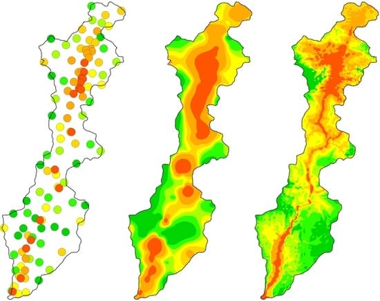
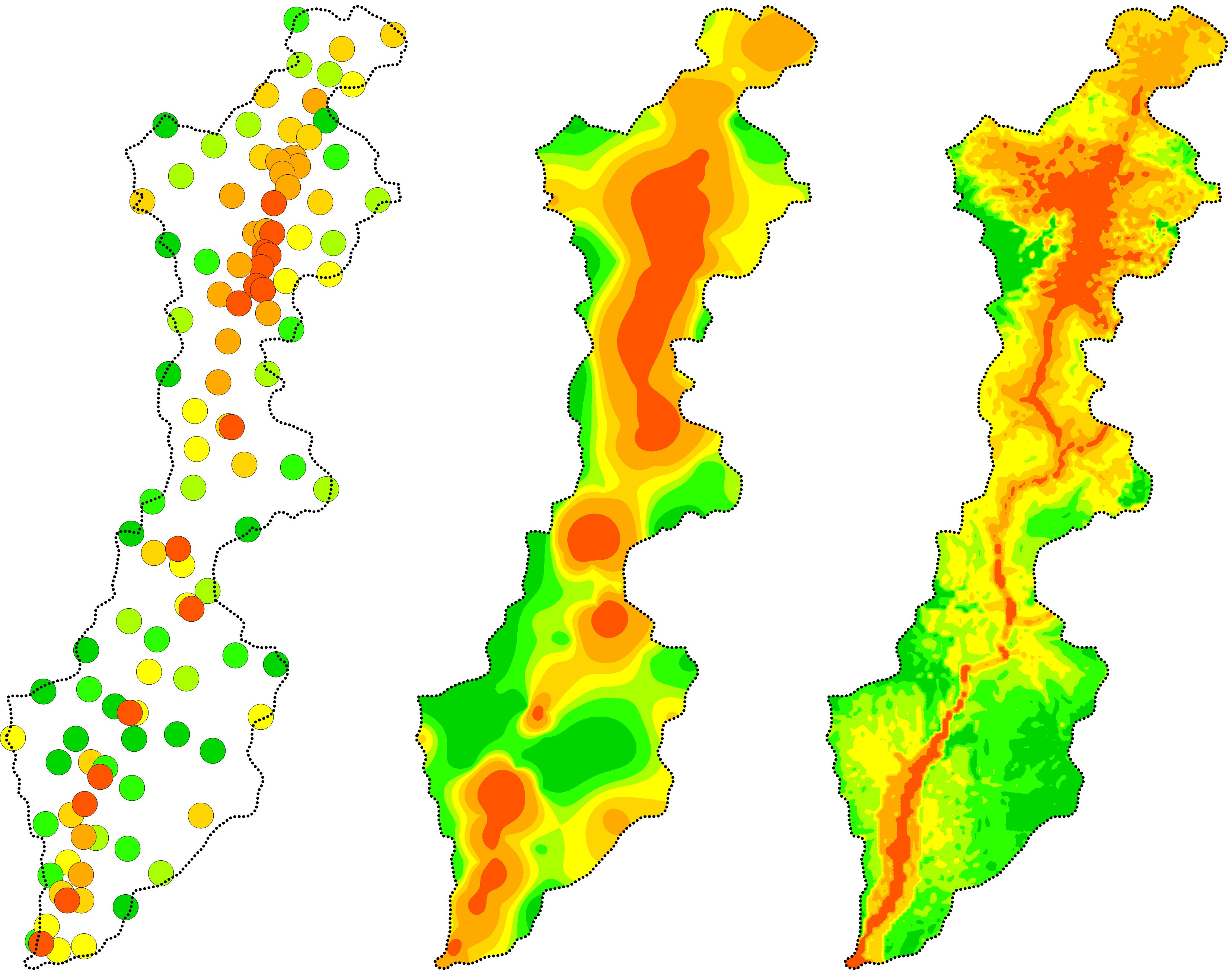
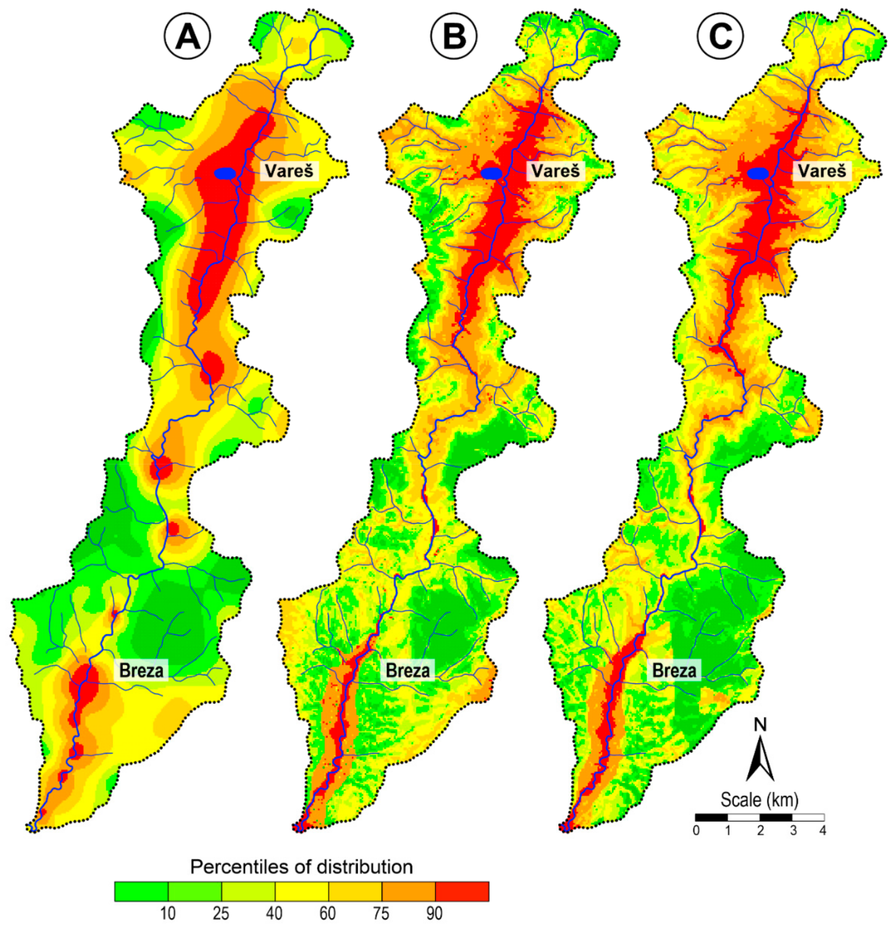
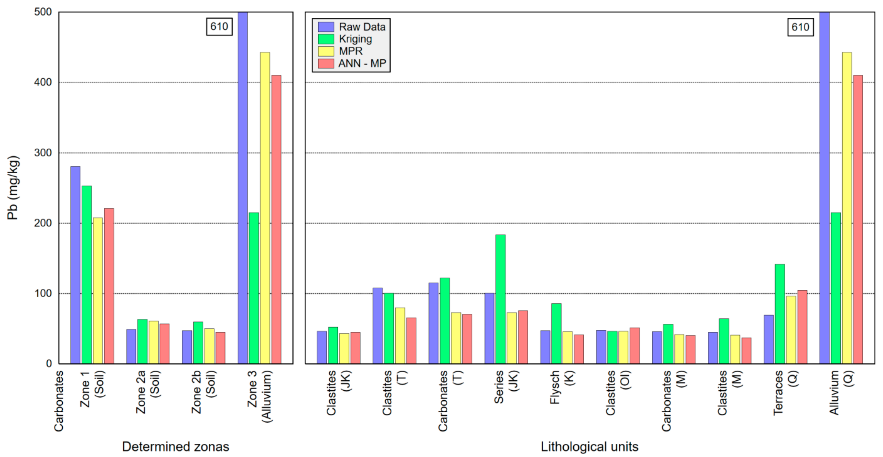
4.3. Spatial Distribution of Pb

Lead is a common anthropogenic chemical element; which concentrations depend on human activities. Distribution of lead within the determined zones and lithological units according to the raw data and prediction methods is presented in Figure A1 (Appendix A). The high concentrations in alluvial soil are consequences of long-lasting mining and smelting activities in the upper part of Valley, around the city Vareš. A fine-grain material is transported by the Stavnja and its tributaries from higher to lower landscapes and embedded to alluvial planes. A study on river Taxco has shown that two main processes are responsible for total Pb variation throughout the year; erosion with discharge processes and dilution connected with different grain-size distribution processes. [69]. It is very interesting for an anthropogenic element that concentrations are higher in the subsoil, but it can be explained by the fact that almost all activities stopped more than 20 years ago [70].

Its concentrations are diverse through the study area, but the evident increase is in the industrial zone and alluvial planes. It can be observed that the difference in predicted values within the raw data and prediction method is present. MPR and ANN-MP are giving very similar results. Kriging, on the other hand, is giving values even lower than 50% in contaminated areas and higher concentrations are found in some lithological units where they are not expected. This could be explained with the appearance of circles in spatial distributions maps (called Bull Eye’s effect). The Box-Cox transformation used in all three prediction methods brings more accurate results but also improves the symmetry of data distribution and variance stabilization. It could be observed that the anomaly is on quaternary alluvium, where maximal values reach 610 mg/kg (raw data). Along the entire valley, natural enrichment is about 50 mg/kg. This means that human impact increased its concentration between four and 12 times in this lithological unit according to all prediction methods.

Predicting the spatial distribution of Pb in soil and identifying hotspots with its high concentration using three prediction methods: (A) Kriging, (B) multiple polynomial regression (MPR), and (C) artificial neural network-multilayer perceptron (ANN-MLP) are presented in Figure 5. These prediction models are showing an arrangement in concentrations across the study area after using Box-Cox transformation and average values of surface soil and subsoil. For a graphical display of spatial distribution, the maps with percentile distribution have been used, where different colours represent different concentration arrangements. The spatial distribution pattern is reconstructing its main pathway in the study area. These models are providing a similar pattern of Pb concentration hotspots, indicating the same source of contamination. In the upper part of the study area, all three models are providing the same shape of contamination areola. This part of the study area is surrounded by steep hills, and the contamination of areola is influenced by the main wind direction, which is N–S. The river transport of clay fine grain is transported down into alluvial sediments. The eroded material has been transported and embedded in the alluvial plain of urban zone Breza, where intensive agriculture occurs. Two advanced methods, MPR and ANN-MLP include lots of geospatial data and those methods are showing a more realistic arrangement in concentrations than models obtained by Kriging, where only sparse soil measurements are included. On the other hand, their similarities are reconfirmation, refinement and at the same time validation of different models. The models are repeatable, what is another success in such modelling.

Determination of the real impact of Pb in the study area can be obtained by comparing the measured data recommended by VROM 2009. According to the VROM 2009, a target value of Pb is 85 mg/kg and the intervention value 530 mg/kg. Its maximum concentrations (880–1700 mg/kg) exceed the intervention values in Zone 1 and alluvial sediments more than three times and target values for 20 times.

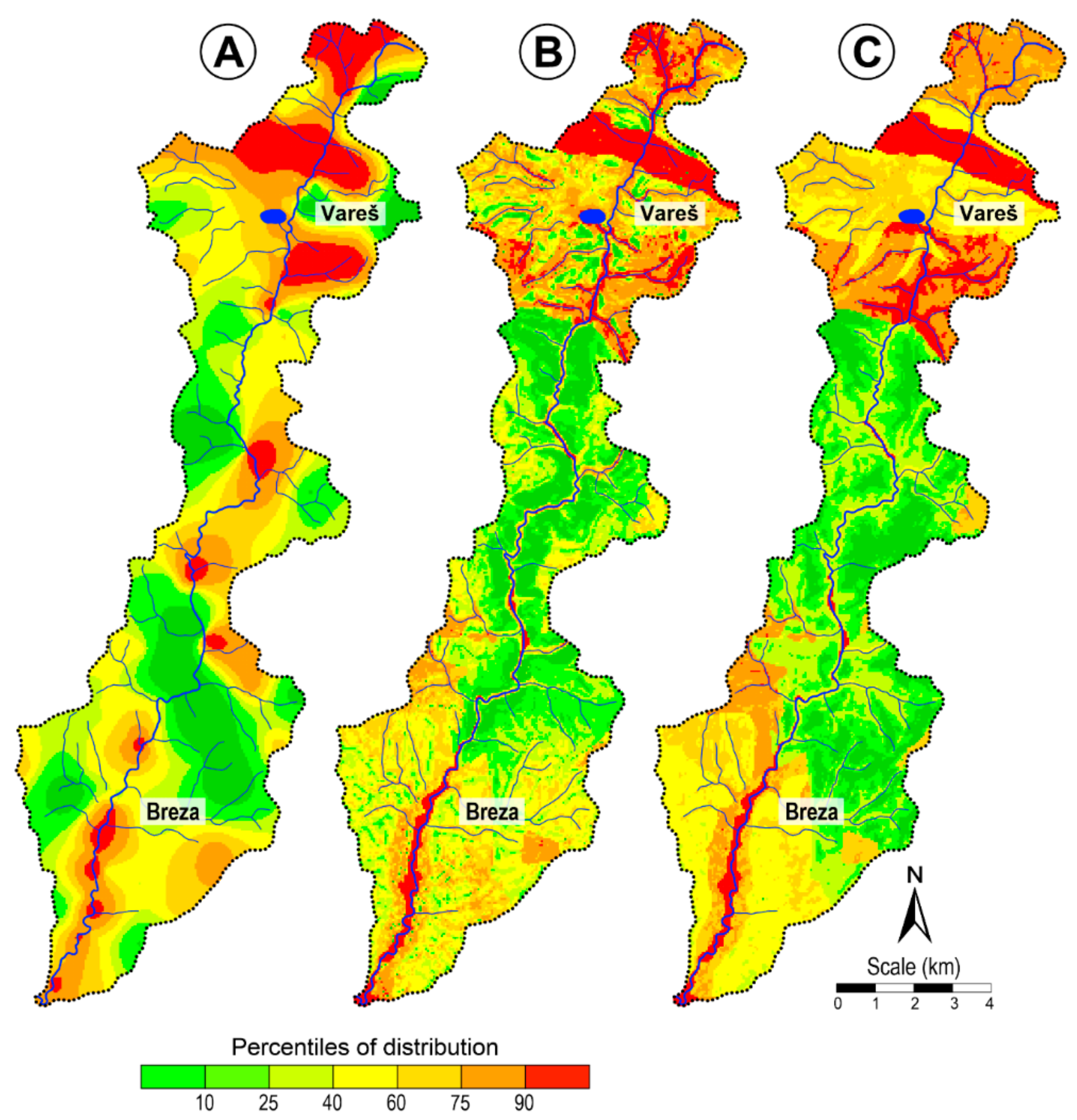
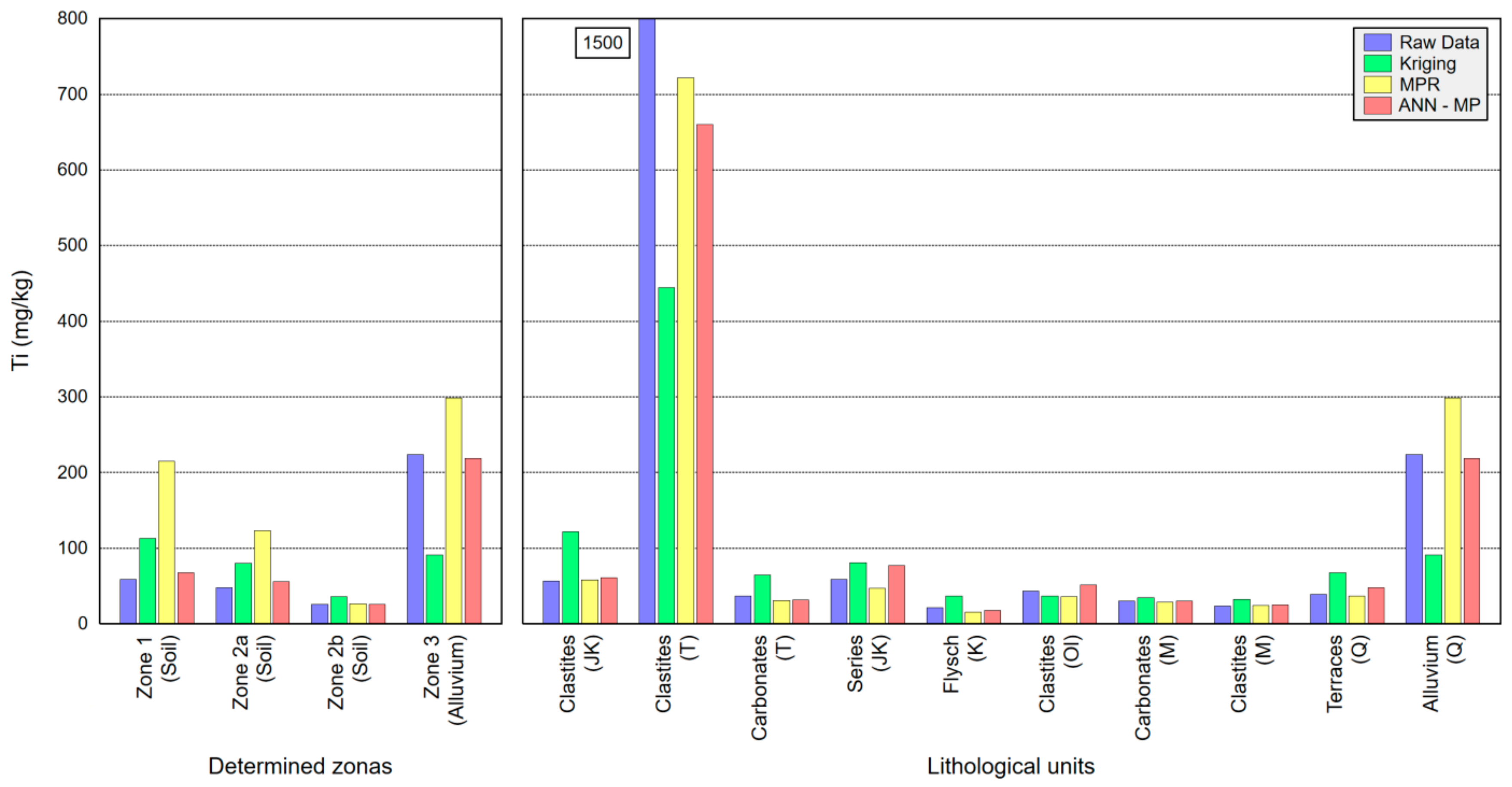
4.4. Spatial Distribution of Ti

Contrary to the Pb anthropogenic distribution, the level of Ti in soil depends only on a natural background. Distribution of Ti within the lithological units according to the raw data and prediction methods after using the Box-Cox transformation is presented in Figure A2. It is clearly visible that a significant increase in concentrations is related to the specific lithological unit, the Triassic Clastites, spilites, and tuff. Such parental material contains much more Ti than other isolated units in the study area. Considering its tendency of incorporation into the finest clay size particles, Ti has been transported far from the source of contamination by water. The significant increase is present in alluvial deposits fined in the morphologically lower part of the study area. Prediction values obtained by kriging are much lower than values obtained by MPR and ANN-MP in the units with higher Ti level and its main source in the soil. In these two units, the predicted values obtained by MPR are higher than ANN-MP values. As was expected, the artificial intelligence offers the best results.

Prediction models of Ti spatial distribution isolate the highest concentrations in Triassic Clastites, spilites and tuffaceous sandstones, but also along with the entire alluvial sediments (JK clastic carbonate series) (Figure 6). ANN-MP and MPR provide significant information according to their transportation downriver. In the upper part of the study area, the high concentrations of Ti are conducted to almost all tributaries. The spatial distributions show that materials with Ti particles concentrate on the lower parts, which means, the finest grains are transported and embed into alluvial sediments. The Southern part of the study area (Oligocene Clastite complex, Miocene Clastitc series and Miocene carbonates with coal layers) is enriched too. At several places, kriging provides its concentration in the form of concentric circles, which is incorrect comparing with the other two models.

4.5. ANN-MP Model Validation and Applicability in Various Case Studies

From the very beginning of the method development, we wanted to achieve three following attributes: (1) to construct a very stable ANN-MP model; (2) model repeatability, and (3) model application within geochemically and morphologically diverse study areas. This means that once the model is prepared, it must be applicable in other case studies under similar conditions (such as input data, number of hidden units, number of training networks), solving a problem of the spatial distribution of particular trace elements or their geochemical groups. In order to show a validation and ANN-MP model applicability, one test site in Macedonia had been selected.

The study area is in the south-central part of Macedonia, about 100 km south of Skopje. The city is well known by Ferro-Nickel smelter FENI, but also famous for its vineyards and it is the main vine production region in Macedonia. The complete investigated region (360 km²) was covered by 172 sampling sites [18,71].

Construction of geochemical maps using universal kriging methods (Figure 7A) is quite useful in the determination of distribution patterns, but around the low and high points appear the circles so-called Bull’s eye effect. This can only be solved by a denser sampling grid. Applying the ANN-MP (Figure 7B), the above effect has been avoided and geochemical contamination maps show more realistic distribution, from the geological point of view. According to the presented results, the model stability and applicability could be confirmed, representing a milestone in geochemical map construction.

5. Conclusions

Along the Stavnja Valley, intensive mining and smelting activities have occurred for more than 100 years. Diverse mineral occurrence, specific geological settings, and geomorphological features make this study area interesting for applying advanced mathematical methods. The study area has been a place of intensive military operation during the last war, 1992–1995, which resulted in numerous remaining minefields, and made this research more complex. According to our experience, such sampling should be done in a group of two or three people maximum, if possible, with one local. The distance between two people should be about 40 m, in case that one activates the mine, another can help. One rout should be used in both directions: to the sampling site and on the way back. If possible, existing routes or hard surfaces should be used for walking. It can be concluded that there is no one rule or several rules for safe sampling in the remaining minefields but only recommendations. It can be concluded; the only rule is that there is no rule. Due to the obvious reasons, several site positions intended for this survey had to be removed accordingly.

Detailed inspection of Pb which is a typical anthropogenic element and Ti typical geogenic element helped in the reconstruction of its main pathway in the study area. The spatial distribution obtained by linear (MPR) and nonlinear method (ANN-MPR) successfully solved a problem of contamination along the river represents an anisotropic appearance between the isotropic lithological units and cannot be solved completely by standard interpolation kriging methods, based only on sparse soil measurements. Their arrangement in concentration across the Valley are more visually realistic and imagery, because they include more geospatial and geomorphological data such as geological background, land use, aspect, slope, altitude, etc. Such models will help us to understand processes that happened in a certain period and improve the data interpretation.

Various modelling techniques help us in the reconstruction of different processes that influenced the entire area. Their main purpose is not only the isolation of hotspots with the highest concentrations but simultaneously they distinguish the distribution pathways of a particular element or group of elements. The applied models are repeatable, which means that very similar spatial distribution can be obtained under the same conditions unrestrictedly. Also, a very important characteristic of each particular modelling is that one model isolates all hotspots simultaneously. In another hand, their similarities are reconfirmation, refinement and at the same time validation of different models.

Advanced modelling represents a milestone in geochemical investigations and mapping itself. The main advantages of those methods are, first of all, that we can construct very eventful and complete maps with the spatial distribution of particular elements or geochemical association, sampling at high-risk sites can be avoided (such as the Stavnja valley), and a number of sampling sites can be reduced while the maps can still remain very qualitative. Such models have a significant contribution to understanding the decomposing mechanism of mining waste and its environmental impact as well as used in remediation processes of the affected areas.

References

1. Schumm, S.A. The Fluvial System; John Wiley & Sons: New York, NY, USA, 1977; 338p. [Google Scholar]
2. Ferreira, V.; Koricheva, J.; Duarte, S.; Niyogi, D.K.; Guerold, F. Effects of anthropogenic heavy metal contamination on litter decomposition in streams—A meta-analysis. Environ. Pollut. 2016, 210, 261–270. [Google Scholar] [CrossRef] [PubMed]
3. Šajn, R.; Halamić, J.; Peh, Z.; Galović, L.; Alijagić, J. Assessment of the natural and anthropogenic sources of chemical elements in alluvial soils from the Drava River using multivariate statistical methods. J. Geochem. Explor. 2011, 110, 278–289. [Google Scholar] [CrossRef]
4. Yi, Q.; Dou, X.D.; Huang, Q.R.; Zhao, X.Q. Pollution Characteristics of Pb, Zn, As, Cd in the Bijiang River. Procedia Environ. Sci. 2012, 13, 43–52. [Google Scholar] [CrossRef] [Green Version]
5. Zhao, X.; Dai, J.; Wang, J. GIS-based evaluation and spatial distribution characteristics of land degradation in Bijiang watershed. SpringerPlus 2013, 2, 1–8. [Google Scholar] [CrossRef] [Green Version]
6. Pavlowsky, R.T.; Lecce, S.A.; Owen, M.R.; Martin, D.J. Legacy sediment, lead, and zinc storage in channel and floodplain deposits of the Big River, Old Lead Belt Mining District, Missouri, USA. Geomorphology 2017, 299, 54–75. [Google Scholar] [CrossRef]
7. Singh, K.P.; Basant, N.; Malik, A.; Jain, G. Modelling the performance of “up-flow anaerobic sludge blanket” reactor based wastewater treatment plant using linear and nonlinear approaches—A case study. Anal. Chim. Acta 2010, 658, 1–11. [Google Scholar] [CrossRef]
8. Navarro, M.C.; Pérez-Sirvent, C.; Martínez-Sánchez, M.J.; Vidal, J.; Tovar, P.J.; Bech, J. Abandoned mine sites as a source of contamination by heavy metals: a case study in a semi-arid zone. J. Geochem. Explor. 2008, 96, 183–193. [Google Scholar] [CrossRef]
9. Dudka, S.; Adriano, D.C. Environmental impacts of Metal Ore Mining and Processing: A Review. J. Environ. Qual. 1997, 26, 590–602. [Google Scholar] [CrossRef]
10. Shallari, S.; Schwartz, C.; Hasko, A.; Morel, J.L. Heavy metals in soils and plants of serpentine and industrial sites of Albania. Sci. Total Environ. 1998, 209, 133–142. [Google Scholar] [CrossRef]
11. Chopin, E.I.B.; Alloway, B.J. Distribution and mobility of trace elements in soils and vegetation around the mining and smelting areas of Tharsis, Ríotinto and Huelva, Iberian Pyrite Belt, SW Spain. Water Air Soil Pollut. 2007, 182, 245–261. [Google Scholar] [CrossRef]
12. Al-Khashman, O.A.; Shawabkeh, R.A. Metal distribution in urban soil around steel industry beside Queen Alia Airport, Jordan. Environ. Geochem. Health 2009, 31, 717–726. [Google Scholar] [CrossRef] [PubMed]
13. Budkovič, T.; Šajn, R.; Gosar, M. Environmental impact of active and abandoned mines and metal smelters in Slovenia. Geologija 2003, 46, 135–140. [Google Scholar] [CrossRef]
14. Lee, C.H. Assessment of contamination load on water, soil and sediment affected by the Kongjujiel mine drainage, Republic of Korea. Environ. Geol. 2003, 44, 501–515. [Google Scholar] [CrossRef]
15. Bhattacharya, P.; Ahmed, K.M.; Hasan, M.A.; Broms, S.; Fogelström, J.; Jacks, G.; Sracek, O.; Von Brömssen, M.; Routh, J. Mobility of arsenic in groundwater in a part of Brahmanbaria district, NE Bangladesh. In Managing Arsenic in the Environment: From Soils to Human Health; Naidu, R., Smith, E., Owens, G., Bhattacharya, P., Nadebaum, P., Eds.; CSIRO Publishing: Collingwood, Australia, 2006; pp. 95–115. [Google Scholar]
16. Bretzel, F.; Calderisi, M. Metal contamination in urban soils of coastal Tuscany (Italy). Environ. Monit. Assess. 2006, 118, 319–335. [Google Scholar] [CrossRef]
17. Gomes, M.E.P.; Favas, P.J.C. Mineralogical controls on mine drainage of the abandoned Ervedosa tin mine in north-eastern Portugal. Appl. Geochem. 2006, 21, 1322–1334. [Google Scholar] [CrossRef]
18. Stafilov, T.; Šajn, R.; Pančevski, Z.; Boev, B.; Frontasyeva, M.V.; Strelkova, L.P. Heavy metal contamination of topsoils around a lead and zinc smelter in the Republic of Macedonia. J. Hazard. Mater. 2010, 175, 896–914. [Google Scholar] [CrossRef]
19. Alijagić, J.; Šajn, R. Distribution of chemical elements in an old metallurgical area, Zenica (Bosnia and Herzegovina). Geoderma 2010, 162, 71–85. [Google Scholar]
20. Khosravi, Y.; Zamanni, A.A.; Parizanganeh, A.H.; Yaftin, M.R. Assessment of spatial distribution pattern of heavy metals surrounding a lead and zinc production plant in Zanjan Province, Iran. Geoderma Reg. 2018, 12, 10–17. [Google Scholar] [CrossRef]
21. McBratney, A.B.; Mendonça Santos, M.L.; Minasny, B. On digital soil mapping. Geoderma 2003, 117, 3–52. [Google Scholar] [CrossRef]
22. Scull, P.; Franklin, J.; Chadwick, O.A.; McArthur, D. Predictive soil mapping: A review. Prog. Phys. Geogr. 2003, 27, 171–197. [Google Scholar] [CrossRef] [Green Version]
23. Bagheri Bodaghabadi, M.; Martínez-Casasnovas, J.A.; Salehi, M.H.; Mohammadi, J.; Esfandiarpoor Borujeni, I.; Toomanian, N.; Gandomkar, A. Digital Soil Mapping Using Artificial Neural Networks and Terrain-Related Attributes. Pedosphere 2015, 25, 580–591. [Google Scholar] [CrossRef] [Green Version]
24. Zhang, G.; Liu, F.; Song, X. Recent progress and future prospect of digital soil mapping: A review. J. Integr. Agric. 2017, 16, 2871–2885. [Google Scholar] [CrossRef]
25. Lagacherie, P.; McBratney, A.B. Spatial soil information systems and spatial soil inference systems: Perspectives for Digital Soil Mapping. In Digital Soil Mapping—An Introductory Perspective, Developments in Soil Science; Lagacherie, P., McBratney, A.B., Voltz, M., Eds.; Elsevier: Amsterdam, The Netherlands, 2007; pp. 3–24. [Google Scholar]
26. Alijagić, J. Application of multivariate statistical methods and artificial neural network for separation natural background and influence of mining and metallurgy activities on distribution of chemical elements in the Stavnja Valley (Bosnia and Herzegovina). Ph.D. Thesis, University of Nova Gorica, Nova Gorica, Slovenia, 2013. [Google Scholar]
27. Hengl, T.; Heuvelink, G.B.M.; Rossiter, D.G. About regression-kriging: From equations to case studies. Comput. Geosci. 2007, 33, 1301–1315. [Google Scholar] [CrossRef]
28. Mali, M.; Dell’Anna, M.M.; Rossiter, D.G.; Notarnicola, M.; Damiani, L.; Mastrorilli, P. Combining cheometric tools for assessing hazard sources and factors simultaneously in contaminated areas. Case study; “Mar Piccolo” Taranto (South Italy). Chemosphere 2017, 184, 784–794. [Google Scholar] [CrossRef]
29. Pamić, J.; Pamić, O.; Olujić, J.; Milojević, R.; Veljković, D.; Kapeler, I. Basic Geological Map of SFRJ, Sheet Vareš 1:100.000 (Interpreter); Federal Geological Survey: Belgrade, Serbia, 1978; 68p.
30. Palinkaš, L.A.; Šoštarić, S.B.; Palinkaš, S.S. Metallogeny of the Northwestern and Central Dinarides and Southern Tisia. Ore Geol. Rev. 2008, 34, 501–520. [Google Scholar] [CrossRef]
31. Stafilov, T.; Šajn, R.; Boev, B.; Cvetković, J.; Mukaetov, D.; Andreevski, M.; Lepitkova, S. Distribution of some elements in surface soil over the Kavadarci region, Republic of Macedonia. Environ. Earth Sci. 2010, 61, 1515–1530. [Google Scholar] [CrossRef]
32. Šajn, R. Using attic dust and soil for the separation of anthropogenic and geogenic elemental distributions in an old metallurgic area (Celje, Slovenia). Geochem. Explor. Environ. Anal. 2005, 5, 59–67. [Google Scholar] [CrossRef]
33. Šajn, R. Factor analysis of soil and attic-dust to separate mining and metallurgy influence, Meža Valley, Slovenia. Math. Geol. 2006, 38, 735–747. [Google Scholar] [CrossRef]
34. Salminen, R.; Batista, M.J.; Bidovec, M.; Demetriades, A.; De Vivo, B.; De Vos, W.; Duris, M.; Gilucis, A.; Gregorauskiene, V.; Halamić, J.; et al. Geochemical Atlas of Europe, Part 1, Background Information, Methodology and Maps; Geological Survey of Finland: Espoo, Finland, 2005; 526p. [Google Scholar]
35. FAO. Guidelines for Soil Profile Descriptions, 4th ed.; FAO: Rome, Italy, 2006; 97p. [Google Scholar]
36. ACME. Available online: http://acmelab.com (accessed on 15 September 2011).
37. Google Earth Maps. Available online: http://earth.google.com (accessed on 17 February 2013).
38. SRTM. Available online: http://srtm.csi.cgiar.org (accessed on 28 January 2013).
39. Gringarten, E.; Deutsch, C.V. Teacher’s aide: Variogram interpretation and modelling. Math. Geol. 2001, 33, 507–534. [Google Scholar] [CrossRef]
40. Krige, D.G. A statistical approach to some basic mine valuation problems on the Witwatersrand. J. Chem. Metall. Min. Soc. South Afr. 1951, 52, 119–139. [Google Scholar]
41. Krige, D.G. On the departure of ore value distributions from lognormal models in South African gold mines. J. Chem. Metall. Min. Soc. South Afr. 1960, 61, 231–244. [Google Scholar]
42. Rose, A.W.; Hawkes, H.E.; Webb, J.S. Geochemistry in Mineral Exploration, 2nd ed.; Academic Press: London, UK, 1979; 657p. [Google Scholar]
43. Zhang, C.S.; Zhang, S.; Zhang, L.C.; Wang, L.J. Background contents of heavy metals in sediments of the Changjiang River system and their calculation methods. J. Environ. Sci. 1995, 7, 422–429. [Google Scholar]
44. Zhang, C.S.; Selinus, O. Statistics and GIS in environmental geochemistry—Some problems and solutions. J. Geochem. Explor. 1998, 64, 339–354. [Google Scholar] [CrossRef]
45. Box, G.E.P.; Cox, D.R. An analysis of transformations. J. R. Stat. Soc. Ser. B 1962, 26, 211–252. [Google Scholar] [CrossRef]
46. Jobson, J.D. Applied Multivariate Data Analysis. Vol. I: Regression and Experimental Design; Springer-Verlag: New York, NY, USA, 1991; 662p. [Google Scholar]
47. Zhang, C.S.; Zhang, S. A robust-symmetric mean: A new way of mean calculation for environmental data. Geo J. 1996, 40, 209–212. [Google Scholar] [CrossRef]
48. Zhang, C.S.; Selinus, O.; Schedin, J. Statistical analyses on heavy metal contents in till and root samples in an area of southeastern Sweden. Sci. Total Environ. 1998, 212, 217–232. [Google Scholar] [CrossRef]
49. McGrath, D.; Zhang, C.; Carton, O.T. Geostatistical analyses and hazard assessment on soil lead in Silvermines area, Ireland. Environ. Pollut. 2004, 127, 239–248. [Google Scholar] [CrossRef]
50. Li, Y.; Zhu, A.; Shi, Z.; Liu, J.; Du, F. Supplemental sampling for digital soil mapping based on prediction uncertainty from both the feature domain and the spatial domain. Geoderma 2016, 284, 73–84. [Google Scholar] [CrossRef]
51. Carlon, C.; Critto, A.; Marcomini, A.; Nathanail, P. Risk based characterisation of contaminated industrial site using multivariate and geostatistical tools. Environ. Pollut. 2001, 111, 417–427. [Google Scholar] [CrossRef]
52. Theodossiou, N.; Latinopoulos, P. Evaluation and optimisation of groundwater observation networks using the Kriging methodology. Environ. Model. Softw. 2006, 21, 991–1000. [Google Scholar] [CrossRef]
53. Webster, R.; Oliver, M.A. Geostatistics for Environmental Scientists; John Wiley and Sons Ltd.: Chichester, UK, 2001; 271p. [Google Scholar]
54. Oliver, M.A.; Webster, R. A tutorial guide to geostatistics: Computing and modelling variograms and kriging. Catena 2014, 113, 56–69. [Google Scholar] [CrossRef]
55. Žibret, G.; Šajn, R. Hunting for geochemical associations of elements: Factor analysis and self-organising maps. Math. Geol. 2010, 42, 681–703. [Google Scholar] [CrossRef]
56. Rosenblatt, F. The perceptron: A probabilistic model for information storage and organization in the brain. Psychol. Rev. 1958, 65, 386–408. [Google Scholar] [CrossRef] [PubMed] [Green Version]
57. ASCE. Available online: https://www.asce.org/ (accessed on 28 May 2010).
58. Du, K.L.; Swamy, M.N.S. Neural Networks in an Softcomputing Framework; Springer–Verlag: London, UK, 2006; 566p. [Google Scholar]
59. Agirre-Basurko, E.; Ibarra-Berastegi, G.; Madariaga, I. Regression and multilayer perceptron-based models to forecast hourly O3 and NO2 levels in the Bilbao area. Environ. Model. Softw. 2006, 21, 430–446. [Google Scholar] [CrossRef]
60. Danandeh, M.A.; Nourani, V. A Pareto-optimal moving average-multigene genetic programming model for rainfall-runoff modelling. Environ. Model. Softw. 2017, 92, 239–251. [Google Scholar] [CrossRef]
61. Žibret, G.; Šajn, R.; Alijagić, J.; Stafilov, T. Use of neural networks in the geochemical data interpretation. Zeitschrift für Geologische Wissenschaften 2012, 40, 253–266. [Google Scholar]
62. Kelechi, A.C. Regression and Principal Component Analyses: A Comparison Using Few Regressors. Am. J. Math. Stat. 2012, 2, 1–5. [Google Scholar] [CrossRef] [Green Version]
63. Ostertagová, E. Modelling using polynomial regression. Procedia Eng. 2012, 48, 500–506. [Google Scholar] [CrossRef] [Green Version]
64. Kerrou, J.; Deman, G.; Tacher, L.; Benabderrahmane, H.; Perrochet, P. Numerical and polynomial modelling to assess environmental and hydraulic impacts of the future geological radwaste repository in Meuse site (France). Environ. Model. Softw. 2017, 97, 157–170. [Google Scholar] [CrossRef]
65. Stat Soft, Inc. STATISTICA (Data Analysis Software System), Version 11–Software; Stat Soft, Inc.: Tulsa, OK, USA, 2012; Available online: www.statsoft.com (accessed on 30 January 2020).
66. Golden Software, Inc. Surfer (Surface Mapping System), Ver 11–Software; Golden Software, Inc.: Golden, CO, USA, 2012. Available online: http://www.goldensoftware.com (accessed on 30 January 2020).
67. Abdi-Khangha, M.; Bemani, A.; Naserzadeh, Z.; Zhang, Z. Prediction of solubility of N-alkanes in supercritical CO2 using RBF-ANN and MLP-ANN. J. CO2 Util. 2018, 25, 108–119. [Google Scholar] [CrossRef]
68. Meloun, M.; Sanka, M.; Nemec, P.; Kritkova, S.; Kupka, K. The analysis of soil cores polluted with certain metals using the Box–Cox transformation. Environ. Pollut. 2005, 137, 273–280. [Google Scholar] [CrossRef] [PubMed]
69. Cabrera-Arcega, F.; Armienta, M.A.; Daessle, L.W.; Castillo-Blum, S.E.; Talavera, O.; Dotor, A. Variations of Pb in a mine-impacted tropical river, Taxco, Mexico: Use of geochemical, isotopic and statistical tools. Appl. Geochem. 2009, 24, 162–171. [Google Scholar] [CrossRef]
70. Alijagić, J.; Šajn, R.; Rokavec, D. Impact assessment of mining and metallurgical activities on the distribution of trace elements in the Stavnja Valley, Bosnia and Herzegovina. In Advances in Environmental Research; Daniels, J.A., Ed.; Nova Science Publishers: New York, NY, USA, 2015; pp. 139–200. [Google Scholar]
71. Stafilov, T.; Šajn, R.; Alijagić, J. Distribution of Arsenic, Antimony and Thallium in Soil in Kavadarci and the Environs, Republic of Macedonia. Soil Sediment Contam. 2013, 22, 105–118. [Google Scholar] [CrossRef]
Figure 1. Location of the study area and isolated lithological units.
Minerals 10 00120 g001
Figure 2. Sampling sites with determined zones.
Minerals 10 00120 g002
Figure 3. Regression plots of predicted vs. observed values for Lead and Titanium according to the prediction methods and transformations: ANN-MP (A—Pb/Raw data, B—Pb/Box-Cox values, E—Ti/Raw data, F—Ti/Box-Cox values) and MPR (C—Pb/Raw data, D—Pb/Box-Cox values, G—Ti/Raw data, H—Ti/Box-Cox values).
Minerals 10 00120 g003
Figure 4. Regression plots between prediction methods: ANN-MP vs. Kriging (A—Pb/Raw data values, B—Pb/Box-Cox values, E—Ti/Raw data values, F—Ti/Box-Cox values) and ANN-MP vs. MPR (C—Pb/Raw data values, D—Pb/Box-Cox values, G—Ti/Raw data values, H—Ti/Box-Cox values).
Minerals 10 00120 g004
Figure 5. Spatial distribution of Lead using different predicting methods: (A)—Kriging; (B)—Multiple polynomial regression (MPR); (C)—Artificial neural network—Multilayer perceptron (ANN-MP).
Minerals 10 00120 g005
Figure 6. Spatial distribution of Titanium using different predicting methods: (A)—Kriging; (B)—Multiple polynomial regression (MPR); (C)—Artificial neural network—Multilayer perceptron (ANN-MP).
Minerals 10 00120 g006
Figure 7. Validation method-Distribution of factor scores (As-Sb-Tl) in Kavadarci area (Macedonia): (A)—Kriging; (B)—Artificial neural network—Multilayer perceptron (ANN-MP).
Minerals 10 00120 g007