A Methodology Based on Magnetic Susceptibility to Characterize Copper Mine Tailings

Abstract

This paper intends to validate the application of magnetic techniques, particularly magnetic susceptibility, as sampling tools on a copper tailings terrace, by correlating them analytically. Magnetic susceptibility was measured in both the field and laboratory. Data obtained allowed for designing spatial magnetic susceptibility distribution maps, showing the horizontal variation of the tailings. In addition, boxplots were used to show the variation of magnetic susceptibility and the concentration of the elements analyzed at different depths of the copper tailings terrace. The degree of correlation between magnetic and chemical variables was defined with coefficient R2. The horizontal and vertical variations of magnetic susceptibility, the concentration of elements, and the significant correlations between them show a relationship between magnetic susceptibility and the chemical processes occurring in the tailing management facility, such as pyrite oxidation. Thus, the correlation functions obtained could be used as semiquantitative tools to characterize tailings or other mining residues.

1. Introduction

The treatment of extensively distributed solid wastes generated by metallurgical processes is a challenge for the environmental sustainability of mining regions [1,2]. Soil characterization is a relevant process for subsequent environmental treatments such as decontamination, stabilization, or remediation [3,4]. The physical (pH, density) and the chemical properties of soils are a forcing factor for the growth and pollutant metabolism of plants during phytoremediation, particularly heavy metal content in the sediments at the (superficial) upper levels [5,6]. In this context, heavy metal concentration is commonly determined by a chemical analysis involving a high cost and a long period of analysis [7,8,9]; however, a low-cost and fast-application method is necessary for effective sediment characterization prior to remediation.

For a reliable tailing storage facility characterization, a large number of sampling points is required so that results can be representative, a fact that has been limited due to the extensive economic resources needed. Sampling quality is essential for estimating the extent of contamination on-site and, therefore, establishing intervention requirements to protect human health and the ecosystem integrity [10]. In this regard, sampling design plays a fundamental role in the tailing characterization stage and must be based on the spatial contamination distribution hypothesis formulated from the results of the exploratory phase of the study. This allows for making an appropriate assessment of the site and its management [11,12]. It is necessary to design a sampling methodology to establish their presence in the mineral species contained in the tailings [13,14]. There are no general rules for soil sampling because each site requires a particular strategy. Therefore, it is important to design a scheme appropriate for each of the tailing storage facilities, considering the optimal location of the sampling points. This scheme must be flexible enough to make adjustments during field activities, owing to, for example, lack of access to preselected sites, unforeseen soil formations, and climatic conditions [15]. The characterization stage involves sampling and the analysis of physical and chemical properties to determine the nature, extent, and extension of contamination. These data are essential for developing, projecting, analyzing, and selecting cost effective technologies to mitigate contamination [16].

Magnetic techniques and methodologies are notable for characterizing soils since they can be validated with a small number of fast chemical analyses at a low cost [17,18]. Although the magnetic phenomenon was recognized in the early 19th century, its application in the different fields of science and technology has increased in the last few decades [19,20,21]. The magnetic characterization and mapping of the magnetic susceptibility of soils have been widely applied as a proxy to characterize heavy metals and pollutants in soils in urban and industrial areas [22,23,24,25,26,27,28,29]. This type of study allows for determining the origin and extension of contaminant agents and their effect on natural soils. Magnetic properties, particularly magnetic susceptibility, are useful tools for identifying and describing ferromagnetic elements (Fe, Ni, Cr). They allow an indirect characterization of the study area because a small number of chemical analyses are needed later.

Magnetic susceptibility is the ability of a material to magnetize itself under the effect of an induced magnetic field, which has a range of values characteristic of the different ferromagnetic elements. It is possible to measure this property in the field by using easy-to-use portable susceptometers at a low cost [30]. Despite the wide use of magnetic techniques for natural soil contamination, they have been scarcely used for detecting and determining the concentration of metals present in tailing deposits [31]. Therefore, the application of magnetic techniques is a good alternative for the chemical characterization of tailing storage facilities due to their high resolution and low cost. In addition, these techniques have important advantages such as short measurement time and the repetition of analyses at a low cost.

Several factors take part in the control of the retention and mobility of heavy metals in the soil, mineralogy playing an important role among them [32]. The bioavailability of most of the elements, particularly heavy metals, is determined by adsorption–desorption, complexation, precipitation, and ion-change processes. The most important surfaces involved in soil metal adsorption are active inorganic colloids such as clayey minerals, metal oxides and hydroxides, metal carbonates and phosphates, and organic colloids [33]. Regarding texture, clayey soils retain more metals by adsorption or in the exchange complex of the clayey minerals; on the contrary, sandy soils lack this fixing capacity. In particular, each clay mineral is characterized by a specific surface area value and a degree of electrical decompensation, which influence its ability to adsorb or exchange metals [34].

Chilean mining is paramount for the country’s development and has become part of its identity. Chile has become a world’s copper production leader, with mining being the productive activity contributing most to GDP [35]. However, it also holds a negative aspect due to the large output of residues and toxic wastes resulting from different operations and processes. Copper sulfide ore processing produces residues called tailings, which contain high heavy metal concentrations [36]. Many solid tailing deposits extend for kilometers, their characterization currently being made via chemical analyses at a high cost [9]. There are 742 mine tailing disposal sites in Chile; some of them are abandoned and require an urgent management plan [37]. To propose remediation plans in order to reduce potential risks associated with tailings, their physicochemical and mineralogical characterization is a priority. These data are not available or are rather scarce, as in the case of geochemical data reported by National Geology and Mining Service (SERNAGEOMIN, for its acronym in Spanish) that determined the geochemical characterization of a number of tailing disposal facilities, based on samples from one to four sampling points [10].

The aim of this work is to discard or validate magnetic susceptibility measurement as a technique for determining the contaminants, concentrations, and/or mobility of the elements in tailing storage facilities. This study, conducted by examining copper mine tailings, intends to validate the techniques measuring magnetic properties as sampling tools, correlating them with a limited number of physicochemical analyses. The objective of this study is to validate the measurement of magnetic susceptibility in the tailing terrace of a copper porphyry-type ore deposit. To attain the objective, heavy metal concentration values in the tailings are correlated with magnetic susceptibility to determine if this technique can be used as a fast and cost effective tool for identifying contaminated areas. Our results are relevant and offer a low cost and effective method to characterize solid wastes generated by copper metallurgical processes prior to their management and treatment in an extensive mining region like northern Chile.

2. Methodology

2.1. Site

This study was conducted in the Atacama Desert, located in Antofagasta Region, Chile. This region is characterized by high solar radiation, high saline soil concentrations, extremely high daytime temperatures, and a wide day–night temperature range. Some areas of the Atacama Desert show zero recorded rainfall in 400 years. In general, rainfall occurs every 100 years. All these conditions produce scarce vegetation. Samples were collected from a copper mine tailings site located at latitude 24°9′58.33″ S and longitude 69°2′33.36″ W, at 3200 masl The terraces where the tailings are disposed show high concentrations of heavy metals such as Cu, Cd, Fe, Zn, Mn, and Pb because the tailings are generated in the sulfide concentration process. The total area of the terrace is about 10,000 m² (135 m × 77 m). This site was used as a tailings dump from 1995 to 2006. Figure 1A,B shows the location of the tailings called CMZ.

CMZ is a copper porphyry with low-grade hypogenic mineralization, where a long continuous supergene enrichment process favored by the predominating tectonic regime during the Upper Oligocene–Lower Miocene [38,39] resulted in the formation of economically exploitable ore deposits. The later decrease of the erosion rate and the increase of regional aridity since the Middle Miocene allowed for the preservation of these ore deposits [40]. Intrusive Oligocene, genetically related to CMZ, includes an early phase of rhyolitic porphyries associated with mineralization and a more intense hypogenic alteration. The later phase corresponds to dioritic porphyries.

According to its mineralization, the ore deposit consists of an upper leached zone associated with quartz–sericitic and copper oxide traces; an oxidation area with brochantite and antlerite; and an extremely sericitized secondary rich zone consisting of pyrite, chalcocine, bornite, covelline, and chalcopyrite. The hypogenic mineralization associated with sericitic alteration and a weak silicification consists mainly of pyrite with small amounts of bornite, chalcopyrite, and molybdenite.

2.2. Sampling In Situ

To collect the samples, the terrace was divided into a grid of 15 m  ×  7 m, covering an internal area of 6615 m², to create 80 equidistant sampling points, as shown in Figure 1C. Due to the rough terrain and to facilitate sample collection, the profiles corresponding to the external points of the terrace were not considered. For the 80 internal points, magnetic susceptibility intensity was measured at three different depths: depth a (0–10 cm deep); depth b (10–20 cm deep); and depth c (20–30 cm deep). This property was used to estimate the points with larger metal concentrations [41]. According to this criterion, 33 sample points were selected.

The samples were collected at the first 30 cm, considering characterization as the preliminary analysis of a phytoremediation system. Plant growth and trace element absorption generally occurred at a 10–30 cm depth [42,43,44].

2.2.1. Sampling Grid Design

The tailings terrace studied is 160 m long and 80 m wide (Figure 1C). For the sampling to include the whole study area, a regular grid was designed, with a 7 m support in the direction of the tailings walls (N05E), while in the W–E direction, they are at a 15 m distance from each other, heading N85E. This area was chosen according to the terrace dimensions so that the sampling could be representative in both directions (nonrandom sampling).

Distances were measured with a 60 m measuring tape, while the direction was obtained with a Brunton compass. The sampling grid was integrated into a geographic data system over a rectified Quickbird image from Google Earth, using ArcGis 10 software.

2.2.2. Sampling

From each tailings sediment site, 1 kg was obtained. The total number of samples amounted to 240. The sediment was extracted with a plastic shovel to avoid altering magnetic measurements. Later, the material collected was stored in clean sealed polyethylene bags, labeled according to site and depth.

Table 1. Example of sample identification.

Type of Sample	Depth (cm)	Sampling Site	Depth Identification	Final Identification
Disaggregated material	0–10	A10	a	A10 a
	10–20	A10	b	A10 b
	20–30	A10	c	A10 c

exemplifies the spatial identification of each tailings sample.

2.3. Measurement Methodology

2.3.1. Magnetic Susceptibility Measurement

Magnetic susceptibility measurements were made with an SM-30 portable susceptometer (Heritage Geophysics, Littleton, CO, USA) to make quick measurements in the field with a 1 × 10⁻⁷ magnetic susceptibility (SI) precision. The measurements were made on dry samples, using the mode 517 of the device at a 43.8 cm³ fixed volume. Magnetic susceptibility measurements were made at the three depths of the 80 sampling points. At each sampling depth, magnetic susceptibility was measured three times at different points. It was possible to check the validity of the susceptometer data by repeating measurements by horizon. Next, the average value was obtained.

2.3.2. pH Measurement

pH was measured in situ with a pH/°C measuring kit, Model HI 99121 (Hanna Instruments, Woonsocket, RI, USA), which is used for measuring both soil pH and a solution prepared with a soil sample directly.

2.3.3. Heavy Metal Concentration Determination

A total of 33 sampling points were selected for chemical analysis. To do this, the following criteria were considered:

(1)

Tailings pH variation; this property conditions metal bioavailability.

(2)

Magnetic susceptibility variation in tailings sediments; samples were selected to make a representative subsampling of all the values observed in the distribution of this property.

(3)

The three depths were established so as to obtain representative results of the whole tailings volume.

Substrate samples, properly labeled and packed in polyethylene bags, were collected. They were oven-dried at 40 °C until reaching a constant weight [45,46]. Gravel-sized rocks (>2 mm) were removed and the remaining particles reduced in size with mortar and pestle. Particles were then screened with a 2-mm sieve (US N° 10 mesh), which is the standard particle size for most soil testing methods [45,47].

Bioavailable Fe, Mn, Zn, Cr, Cu, Cd, and Pb contents were measured with an atomic absorption spectrophotometer (AAS) after extraction by using a diethylenetriaminepentaacetic acid (DTPA) solution [48]. These metals were collected by shaking 0.01 kg of oven-dried soil for 2 h in 20 mL of 0.005 M DTPA. The filtrate was analyzed for Fe, Mn, Zn, Cr, Cu, Cd, and Pb by AAS. Cadmium, copper, chromium, lead, zinc, and iron were measured by ASS, with detection limits of 0.05 mg kg⁻¹ for Cd, Cr and Zn, 4.3 mg kg⁻¹ for Pb, 7.5 mg kg⁻¹ for Cu, and 24 mg kg⁻¹ for Fe. As analysis was conducted separately by hydride generation–atomic absorption spectrometry (HGAAS). Hydride was generated by using a Perkin-Elmer 100 FIAS FIA 100 apparatus (0.005 mg kg⁻¹ detection limit). All solutions were filtered with Whatman GF/C fiberglass filter paper [9].

3. Results

Data selected according to the three criteria above (Section 2.3.3) are shown in

Table 2. Samples selected according to pH classes and magnetic susceptibility variability.

Depth	pH Range	Sample	pH	Soil Κ (µSI)
Depth a 0–10 cm	pH < 5	A30	3.65	389.3
	5 < pH < 6.5	B80	5.45	532.7
		C30	5.32	655.3
		D70	5.43	672.0
		H50	5.65	619.7
		I20	5.12	735.0
		J60	5.97	334.3
	6.5 < pH < 7.5	E40	6.54	520.0
		F60	7.20	655.3
		I80	6.97	679.0
	pH > 7.5	D10	7.99	488.0
Depth b 10–20 cm	5 < pH < 6.5	A30	5.79	618.3
		B70	5.58	1090.0
		D70	5.92	991.0
		E40	6.12	297.0
		E70	6.18	256.8
		G80	6.35	826.0
		I20	6.17	583.0
	6.5 < pH < 7.5	C50	6.58	393.0
		F30	6.89	637.0
		J50	7.02	490.3
	pH > 7.5	D10	7.97	326.7
Depth c 20–30 cm	5 < pH < 6.5	I40	6.35	272.7
	6.5 < pH < 7.5	A50	7.50	186.0
		D70	6.82	434.3
		E40	6.95	160.0
		F20	7.30	816.0
		F60	7.12	682.7
		H70	6.93	1159.0
		I20	6.98	369.3
		J80	7.07	246.3
	pH > 7.5	B30	7.59	364.0
		D10	7.61	479.0

. The spatial distribution of the sampling points for the three depths are shown in Figure 1C.

Table 3. Results of chemical analyses for the first stratum at a 0–10 cm depth.

Site	Cd	As	Zn	Cu	Fe	Ni	Pb	Cr	Soil Κ µSI
	mg·kg−1
A30 a	2.09	26.3	426.7	12,118	33,050	58.3	412.3	27.2	389.3
B80 a	2.10	33.6	446.4	10,395	36,913	96.2	452.3	29.3	532.7
C30 a	1.90	28.3	473.2	12,090	34,653	77.3	376.6	41.2	655.3
D10 a	2.60	21.8	398.8	14,426	31,278	68.4	420.2	17.6	488.0
D70 a	3.20	21.9	306.6	9323	41,923	67.2	289.5	14.8	672.0
E40 a	2.80	32.1	287.2	8225	33,607	88.2	322.2	32.4	520.0
F60 a	4.10	27.3	327.6	8454	34,756	59.6	254.2	29.5	655.3
H50 a	3.70	21.8	333.6	8857	35,656	72.3	322.1	19.3	619.7
I20 a	2.40	32.5	328.8	12,160	36,675	49.4	312.2	22.4	735.0
I80 a	4.20	20.6	425.3	9519	38,137	88.2	453.8	26.7	679.0
J60 a	2.80	23.4	399.5	10,712	33,716	77.3	408.1	33.9	334.3

,

Table 4. Results of chemical analyses for the second stratum at a 10–20 cm depth.

Site	Cd	As	Zn	Cu	Fe	Ni	Pb	Cr	Soil Κ µSI
	mg·kg−1
A30 b	0.848	21.2	373.7	10,728	34,470	32.5	221.2	17.3	618.3
B70 b	1.187	18.3	375.3	8231	33,219	34.6	245.2	12.8	1090.0
C50 b	0.699	15.6	207.7	10,321	30,846	28.3	282.8	21.4	393.0
D10 b	0.899	18.2	450.8	12,658	31,950	41.2	198.4	19.4	326.7
D70 b	0.599	22.4	280.3	16,296	34,781	19.6	187.5	18.6	991.0
E40 b	0.900	23.9	240.6	14,533	31,733	22.2	201.4	22.6	297.0
E70 b	0.352	21.2	200.1	14,701	27,625	28.3	167.4	21.9	256.8
F30 b	0.798	28.3	500.6	9003	37,297	32.2	135.3	18.2	637.0
G80 b	2.298	12.4	271.2	17,203	36,731	31.4	194.9	19.6	826.0
I20 b	1.797	15.6	300.9	11,096	37,095	17.8	217.8	14.3	583.0
J50 b	2.298	17.8	299.5	12,398	38,489	28.2	175.9	18.8	490.3

and

Table 5. Results of chemical analyses for the third stratum at a 20–30 cm depth.

Site	Cd	As	Zn	Cu	Fe	Ni	Pb	Cr	Soil Κ µSI
	mg·kg−1
A50 c	0.698	10.8	225.4	9186	30,433	12.8	222.7	13.6	186.0
B30 c	0.897	17.3	288.3	9798	35,816	23.9	198.6	17.2	364.0
D10 c	1.800	15.4	458.5	12,207	37,001	21.8	178.5	17.4	479.0
D70 c	0.797	14.1	190.9	8181	23,457	17.5	218.7	9.6	434.3
E40 c	0.900	18.3	200.5	8234	30,839	19.8	218.4	22.5	160.0
F 20c	2.791	28.3	495.4	9452	41,652	21.4	198.4	18.4	816.0
F60 c	2.342	17.9	394.4	10,247	36,012	31.2	219.2	28.3	682.7
H70 c	2.021	15.8	313.5	13,939	33,667	18.9	178.9	12.4	1159.0
I20 c	2.396	13.8	483.2	12,591	39,608	24.8	228.9	17.2	369.3
I40 c	1.879	21.2	393.5	13,872	39,540	22.9	178.4	21.9	272.7
J80 c	2.394	17.4	328.4	14,171	34,704	17.9	189.6	19.4	246.3

show the results of the concentration analyses of eight heavy metals (As, Cd, Cr, Cu, Fe, Ni, Pb, and Zn) and the magnetic susceptibility (MS) values for the three points measured in the field. The denomination is based on the names of the wells and the sampling depth, as shown in Table 1.

3.1. Relationship between Magnetic Susceptibility and Depth

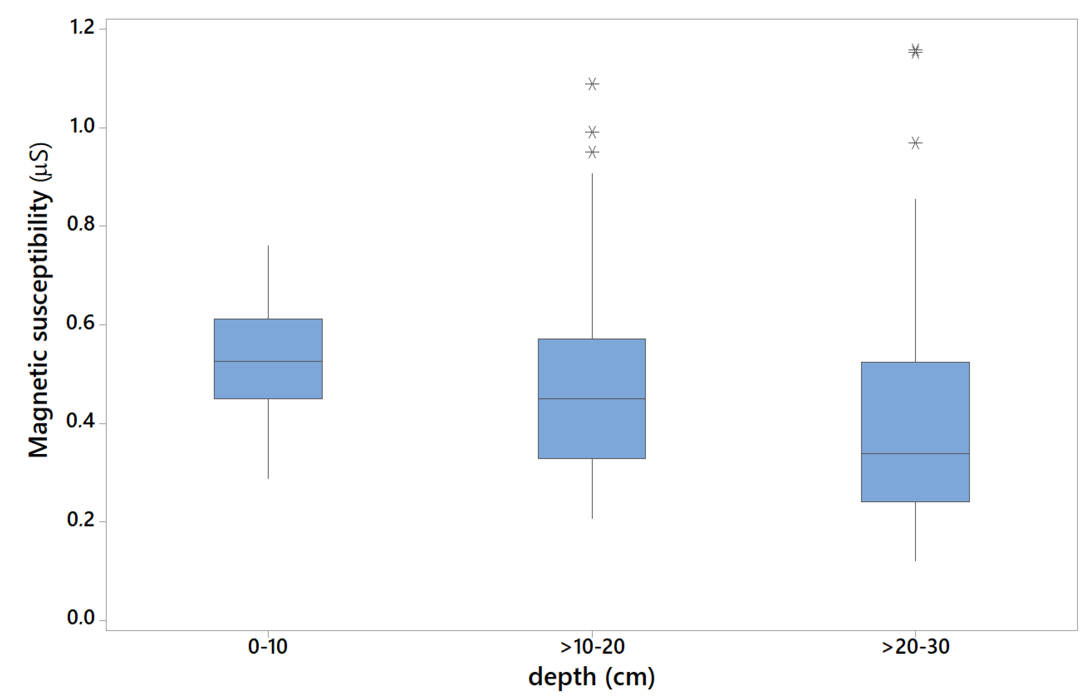
Considering the 240 samples, there is a statistical correlation between sampling depth and magnetic susceptibility. For the three depths, the standard deviation and the variance show high values, indicating a high dispersion of the magnetic susceptibility data measured. The mean value of magnetic susceptibility for the three horizons tends to 411–518 µSI, showing a decrease in depth, as illustrated in Figure 2 and Figure 3, showing a boxplot and an interval plot, respectively. Given a certain relationship between depth and magnetic susceptibility, a hypothesis test was conducted.

The relationship between MS and depth was analyzed with ANOVA. This test shows the influence of one or more factors, in this case depth, over the mean of a continuous variable, in this case MS.

Table 6. Mean value, standard deviation, and confidence interval per sample depth.

Profile	Mean	SD	95% CI
0–10 cm	0.5230	0.1100	(0.4822; 0.5638)
10–20 cm	0.4872	0.1934	(0.4464; 0.5280)
20–30 cm	0.4095	0.2311	(0.3687; 0.4503)

shows the mean, standard deviation, and 95% CI for the mean of each profile. The ANOVA test was conducted with a 95% CI. Results reveal statistically significant differences between at least two groups (df = 2; F = 7.85; p-value = 0.001). According to the results of the Tukey’s post hoc test [49], the group under 30 cm present statistically significant differences in the magnetic susceptibility mean when compared with the other two.

3.2. Relationship between Magnetic Susceptibility and pH

MS decreases as tailing depth increases. Kapikca et al. [50], Hoffmann et al. [51], Boyko et al. [52], and Magiera et al. [53] observed this tendency, associated with the enrichment of anthropogenic particles on the most superficial layers of the soil from nearby industries or plants. The main difference between this study and those mentioned above is the type of soil where samples are collected, since samples are taken from the tailings mass in this study. For this reason, MS decrease is related to chemical processes occurring within the tailings. MS decrease with depth may be explained by the most important reaction in the tailings, i.e., pyrite oxidation (Equations (1)–(3)). As explained by Dold and Fontboté [54], atmospheric oxygen eruption into the system begins sulfide oxidation, in this case pyrite, the main gangue in the ore deposit.

$${\mathrm{FeS}}_2+\frac{7}{2}{\mathrm{O}}_2+{\mathrm{H}}_2\mathrm{O}\to {\mathrm{Fe}}^{+2}+2{\mathrm{SO}}_4^{2-}+2{\mathrm{H}}^{+}$$

(1)

$${\mathrm{Fe}}^{+2}+\frac{1}{4}{\mathrm{O}}_2+{\mathrm{H}}^{+}\to {\mathrm{Fe}}^{3+}+\frac{1}{2}{\mathrm{H}}_2\mathrm{O}$$

(2)

$${\mathrm{Fe}}^{3+}+3{\mathrm{H}}_2\mathrm{O}\to \mathrm{Fe}{\left(\mathrm{OH}\right)}_3+3{\mathrm{H}}^{+}$$

(3)

Pyrite oxidation is the main acidity producer of the system (Equation (1)). The acidity produced by these processes may result in a pH decrease [55,56,57,58,59]. Tailings from copper porphyry-type ore deposits show 1–3% pyrite concentrations [54]. Therefore, ions such as Fe³⁺ precipitate at pH > 3.5. The ferric ion, when not involved in sulfide oxidation, precipitates as secondary mineral such as goethite. Dold and Fontboté [60] conducted chemical, mineralogical, and microbiological analyses on three Chilean copper porphyry ore deposit tailings in different climatic contexts (arid, semiarid, and humid). These tailings were classified as having low sulfidization and carbonate content. The comparison of the behavior of these three tailings shows that the climatic factor controls the direction in which the elements move, free from the chemical reactions in the tailings. For example, in a humid climate, the chemical elements in the tailings move from an oxidizing environment on the upper part to a reducing environment in the direction of the phreatic level. Meanwhile, in regions with an arid climate such as the Atacama Desert, transport is expected to occur in the inverse direction, which is toward a more oxidizing environment due to capillarity, thus forming secondary sulfates on the surface. This effect has also been observed in arid and semiarid environments, favoring oxidation processes and allowing efflorescent mineral formation (hydrated sulfates) on the tailing surface [61,62].

In the tailings studied, horizons a and b show a slightly acid pH, while at depth c, the pH is neutral. This suggests:

(i)

As horizon a is more superficial, pyrite oxidizes, resulting in greater acidity (average pH = 6.1).

(ii)

There is an enrichment of diamagnetic minerals such as silica toward horizon c; i.e., there is a greater neutralization potential (pH = 7.05), which is supported by Si concentration increase with depth.

(iii)

The formation of iron hydroxide should occur at the initial stage (pseudominerals) because, if minerals such as goethite were present in horizon c, the signal would increase owing to the high susceptibility of this mineral, which is not correlated with the MS tendency.

Horizontally, MS shows the highest concentration values at the ends and the lowest concentration values in the middle part of the terrace. Dold [63] indicates that, although tailings particle size is relatively homogeneous, there is a deposition controlled by sedimentological processes resulting in coarse granulometry near the deposition point (sulfides are heavier than silicates). According to this analysis, MS distribution maps show a certain coherence. High MS values may involve the presence of pyrite with positive susceptibility, while low values would be associated with diamagnetic materials such as silica or carbonates.

3.3. Depth Variation of Chemical Elements

As to the variation of chemical elements in the terrace, two factors control element mobility: solubility and pH [64,65]. Solubility is a function of the chemical element concentration of the metal. In lower concentration systems, the elements are more mobile than in those with a higher concentration. Thus, mineralogical composition determines what chemical environment predominates and what elements are liberated and can mobilize [66,67,68]. In the terrace, Cu and Cd increase their concentration towards horizon c, similarly to the pH. These behaviors are consistent, as reported by Dold and Fontboté [54], who determined that in tailings out of operation, the oxidation process occurs in its initial stage. Metals such as Cu, Pb, Cd, Ni, and Ca are quite mobile at a low pH and are adsorbed when pH increases, explaining the lower concentration in horizon a, as compared with horizons b and c. The opposite is observed for Zn behavior, which mainly concentrates in horizon a. Dold and Fontboté [60] observed the same tendency in Zn and Mg in El Salvador tailings, which concentrate on the most superficial layer, corresponding to an evaporitic horizon with a high pH.

3.4. Relationship between Magnetic Susceptibility and Heavy Metal Concentration

This relationship was analyzed with a MARS (multivariate adaptive regression splines) model suitable for this data structure. MARS was calculated by using the earth [69] library of the statistical package R [70], while the other statistical calculations were made with Minitab. Using data from Table 3, Table 4 and Table 5, the relationship between MS and the concentrations of eight heavy metals was analyzed by using MARS, as in other engineering applications [71,72,73,74,75] because it fits these data better than other models [76,77].

The model is a MARS analysis, i.e., a type of regression introduced by Jerome Friedman [78]. It is a nonparametric regression technique that may be understood as a linear model extension automatically modeling nonlinear relationships and interactions between variables. In other words, it automatizes prediction model construction by selecting relevant variables, transforming predictive variables, treating missing values, and avoiding overfitting by means of an autotest. MARS is similar to a linear regression without splines.

It is mainly used for predicting a continuous variable $\stackrel{\rightharpoonup }{y}\left(nx1\right)$, here MS, from a set of explanatory variables $\stackrel{\rightharpoonup }{X}\left(nxp\right)$, here the concentration of heavy metals. So, the MARS model may be represented by the expression $\stackrel{\rightharpoonup }{y}\left(nx1\right)=f\left(\stackrel{\rightharpoonup }{X}\right)+\stackrel{\rightharpoonup }{e}$, where $\stackrel{\rightharpoonup }{e}$ is an $\left(nx1\right)$ error vector.

MARS analysis results in both a linear and a second-grade linear model, without higher-grade models.

In the linear model, a correlation is established between MS and the concentrations of four metals, Cu, Fe, Ni, and Cr, and no correlation obtained with the other heavy metals Cd, As, Zn, and Pb, meaning that the latter are not relevant for MS.

The correlation in this model is given by Equation (4):

MS = 0.55 + 7.2 e⁻⁰⁵ × pmax (0, Cu − 12207) − 5.8 e⁻⁰⁵ × pmax (0, 34756 − Fe) − 0.02 × pmax (0, 31 − Ni) + 0.076 × pmax (0, 19 − Cr)

(4)

where pmax is 0, if the other value is not positive. For example, pmax (0, 19-Cr) becomes 0; i.e., Cr does not influence the correlation until Cr concentration does not exceed 0.19 mg∙kg⁻¹.

MARS model parameters GCV = 0.047, RSS = 0.82, GRSq = 0.26, and RSq = 0.58 show the model goodness of fit, RSq = 0.58, is not low for spread data.

The linear model, represented by pmax functions, shows that as Fe and Ni concentration increases, MS increases up to a certain value and then remains constant. For Cu concentration, MS remains constant up to a certain value and then increases. As for Cr, MS decreases to a certain concentration value and then remains constant (Figure 4).

In the second-grade model, the correlation is established between MS and the concentrations of three metals, Cu, Zn, and Cr, the latter only as a second-order term. No correlation is obtained for the other heavy metals. This means that they are not relevant for MS. The fit is better than the one for the first-order model, with RSq slightly over 0.67. The correlation of the second-grade model is given by Equation (5):

MS = 0.43682171 + 0.00981946 × pmax (0, Zn–287.2) + 0.00981946 × pmax (0, Cu–0.9323) + pmax (0, 287.2–Zn) × Cu − 0.00000040 × pmax (0, Zn–287.2) × Cu − 0.00000089 Zn × pmax (0, 17.3–Cr) × 0.00022912

(5)

MARS model parameters GCV = 0.05631133, RSS = 0.6488601, GRSq = 0.112011, and RSq = 0.670256 show that the model goodness of fit, RSq = 0.67, is better than in the linear model.

Figure 5 shows Zn and Cu linear relationships and Cr second-order relationship.

3.5. MS Advantages over Metal Concentration

The great advantage of susceptibility measurements is their promptness and low cost [79,80,81]. MS was directly measured in the substrate at 0–10, 10–20, and 20–30 cm depths. For each level, MS was measured at least three times at three different points. Then, the average was determined. The sediment was extracted with a plastic shovel to avoid changing magnetic measurements [82]. The technique results in the lowest cost, as compared with every other type of test and is little invasive for the environment. The chemical analysis was more complex, involving soil homogenization, clod disaggregation, and the removal of larger stones and residues. This was followed by clay content drying and sample sieving. Pretreatment for chemical analysis took about 3 days per sample [5,6]. So, preparing the sample for magnetic susceptibility is much simpler than preparing it for a chemical analysis. In addition, time must also be considered. As to MS, it is possible to measure 6 samples in 1 h on an average, considering the pretreatment stage. So, 40 h are required for the 240 sampling points. Thus, by working 8 h/day, 5 days are needed to obtain results. As to concentrations, pretreatment is more demanding and takes longer. For a further description, 6 samples can be collected each hour, the samples requiring at least a 3-day treatment. So, if 48 samples are collected daily, considering 8 h of work/day and 3 additional days for pretreatment, 4 days are required for collecting and treating 48 samples. Hence, for the 240 sampling points 20 days are required. In brief, the MS measurement of 240 points takes 5 days, while collecting and pretreating the 240 samples for measuring concentration takes 20 days. In addition, 3 months are necessary to measure the samples in the laboratory. So, for the time ratio required, concentrations:MS = 110:5 = 22, i.e., 2100% extra time for the characterization process.

Table 7. Time for determining MS and the concentration of 8 heavy metals in 240 samples.

No. of Samples	MS Measurement Time	Time for the Concentration Measurement of 8 Heavy Metals
	Sample Collection and Measurement in Situ	Sample Collection	Pretreatment	Measurement
6	1 h	1 h	3 days	45 days
48	1 day	1 day	3 days	45 days
240	5 days	5 days	15 days	90 days
Time for MS measurement of 240 points	5 days	Time for collection, pretreatment, and concentration measurement of 240 points		110 days

shows the time necessary for measuring magnetic susceptibility and the chemical analysis of 240 sampling points. The chemical analysis considers the determination of eight heavy metals (As, Cd, Cu, Fe, Hg, Pb, and Zn).

The cost of measuring each MS is about 3 USD, while the cost of the chemical analysis of a sample is about 150 USD. For the cost required relationship, chemical analysis:MS = 1:50 USD, i.e., the cost of chemical analyses would be about 4900% higher than the cost of measuring an MS point.

Although it is not possible to measure all the sampling points only with MS, the number of points may decrease if MS can be correlated with the concentration. This renders significant savings, as in this study, where only 33 out of the 240 points were measured, producing savings of more than 30,000 USD.

4. Conclusions

MS measurements may provide further data about soil pollution to estimate the environmental situation in a study area; i.e., magnetic properties show depth variations, which reflect concentration changes, depth being an environmental soil pollution indicator.

A positive linear correlation of magnetic susceptibility with Cr, Fe, Ni, and Cu was observed in the tailings studied, while in the second-grade model a correlation was found for Cu, Zn, and Cr. These heavy metals, well-known as the most hazardous elements, are easily extracted by plants from the soils in the area studied [9]. In addition to traditional geochemical mapping, magnetic susceptibility could be successfully used for determining heavy metal soil pollution in the neighborhood of the site under study.

In the second-grade model, R2 is 0.67. For this kind of problem with spread data, this is not a low value and, therefore, indicates a value correlation between heavy metal concentration and magnetic susceptibility. This correlation is important because the cost of measuring MS is much lower than making chemical analyses for heavy metal concentration. Therefore, an indirect method can be used to assess the presence of heavy metals in tailings without conducting chemical analyses, or perhaps just making a few analyses that may serve as a pattern to calibrate magnetic susceptibility, which has been shown to vary with depth.

The concentration and mobility of chemical elements in the tailings is mainly controlled by pH. The interpretation of this and magnetic data enables detecting the chemical processes in the tailings, such as pyrite oxidation. MS is a good indicator because, as it decreases with depth, it is possible to interpret a greater concentration of diamagnetic minerals toward horizon c, which is complemented by the increasing depth of Cu concentrations.

Tailings sediments correspond to paramagnetic rather than diamagnetic arrangements, where ferromagnetic materials are present in small amounts within the paramagnetic matrix. The grain size of the tailings sediments does not allow a macroscopic recognition. So, for interpreting and understanding the magnetic signal, a detailed mineralogy control is necessary.

The correlation functions obtained can be used as semiquantitative tools for detecting toxic substance formations resulting from chemical reactions.

Magnetic methodologies, along with a small number of chemical analyses on representative samples, make it possible to develop sampling grids with a high spatial resolution at a low cost, thus decreasing costs associated with characterization.

Moreover, the potential use of these measurements to assess the metallic values contained in disposal facilities makes up an issue for further studies.

References

1. Park, I.; Tabelin, C.B.; Jeon, S.; Li, X.; Seno, K.; Ito, M.; Hiroyoshi, N. A review of recent strategies for acid mine drainage prevention and mine tailings recycling. Chemosphere 2019, 219, 588–606. [Google Scholar] [CrossRef] [PubMed]
2. Tabelin, C.B.; Silwamba, M.; Paglinawan, F.C.; Mondejar, A.J.S.; Duc, H.G.; Resabal, V.J.; Opiso, E.M.; Igarashi, T.; Tomiyama, S.; Ito, M.; et al. Solid-phase partitioning and release-retention mechanisms of copper, lead, zinc and arsenic in soils impacted by artisanal and small-scale gold mining (ASGM) activities. Chemosphere 2020, 260, 127574. [Google Scholar] [CrossRef] [PubMed]
3. Huyen, D.T.; Tabelin, C.B.; Thuan, H.M.; Dang, D.H.; Truong, P.T.; Vongphuthone, B.; Kobayashi, M.; Igarashi, T. The solid-phase partitioning of arsenic in unconsolidated sediments of the Mekong Delta, Vietnam and its modes of release under various conditions. Chemosphere 2019, 233, 512–523. [Google Scholar] [CrossRef] [PubMed]
4. Huyen, D.T.; Tabelin, C.B.; Thuan, H.M.; Dang, D.H.; Truong, P.T.; Vongphuthone, B.; Kobayashi, M.; Igarashi, T. Geological and geochemical characterizations of sediments in six borehole cores from the arsenic-contaminated aquifer of the Mekong Delta, Vietnam. Data Brief. 2019, 25, 104230. [Google Scholar] [CrossRef] [PubMed]
5. Lam, E.J.; Cánovas, M.; Gálvez, M.E.; Montofré, Í.L.; Keith, B.F.; Faz, Á. Evaluation of the phytoremediation potential of native plants growing on a copper mine tailing in northern Chile. J. Geochem. Explor. 2017, 182, 210–217. [Google Scholar] [CrossRef]
6. Lam, E.J.; Gálvez, M.E.; Cánovas, M.; Montofré, Í.L.; Keith, B.F. Assessment of the adaptive capacity of plant species in copper mine tailings in arid and semiarid environments. J. Soils Sedim. 2017, 18, 2203–2216. [Google Scholar] [CrossRef]
7. Acosta, J.A.; Faz, A.; Martínez-Martínez, S.; Zornoza, R.; Carmona, D.; Kabas, S. Multivariate statistical and GIS-based approach to evaluate heavy metals behavior in mine sites for future reclamation. J. Geochem. Explor. 2011, 109, 8–17. [Google Scholar] [CrossRef]
8. Martin-Crespo, T.; Gomez-Ortiz, D.; Martín-Velázquez, S.; Martínez-Pagán, P.; De Ignacio, C.; Lillo, J.; Faz, Á. Geoenvironmental characterization of unstable abandoned mine tailings combining geophysical and geochemical methods (Cartagena-La Union district, Spain). Eng. Geol. 2018, 232, 135–146. [Google Scholar] [CrossRef]
9. Lam, E.J.; Gálvez, M.E.; Cánovas, M.; Montofré, I.L.; Rivero, D.; Faz, A. Evaluation of metal mobility from copper mine tailings in northern Chile. Environ. Sci. Pollut. Res. 2016, 23, 11901–11915. [Google Scholar] [CrossRef]
10. Lam, E.J.; Montofré, I.L.; Álvarez, F.A.; Gaete, N.F.; Poblete, D.A.; Rojas, R.J. Methodology to Prioritize Chilean Tailings Selection, According to Their Potential Risks. Int. J. Environ. Res. Pub. Heal. 2020, 17, 3948. [Google Scholar] [CrossRef]
11. Lark, M.; Hamilton, E.; Kaninga, B.; Maseka, K.K.; Mutondo, M.; Sakala, G.M.; Watts, M.J. Nested sampling and spatial analysis for reconnaissance investigations of soil: An example from agricultural land near mine tailings in Zambia. Eur. J. Soil Sci. 2017, 68, 605–620. [Google Scholar] [CrossRef] [Green Version]
12. Constantinescu, P.; Neagoe, A.; Nicoara, A.; Grawunder, A.; Ion, S.; Onete, M.; Iordache, V. Implications of spatial heterogeneity of tailing material and time scale of vegetation growth processes for the design of phytostabilization. Sci. Total Environ. 2019, 692, 1057–1069. [Google Scholar] [CrossRef] [PubMed]
13. Corriveau, M.; Jamieson, H.E.; Parsons, M.B.; Campbell, J.; Lanzirotti, T. Direct characterization of airborne particles associated with arsenic-rich mine tailings: Particle size, mineralogy and texture. Appl. Geochem. 2011, 26, 1639–1648. [Google Scholar] [CrossRef]
14. Khelfaoui, M.; Medjram, M.S.; Kabir, A.; Zouied, D.; Mehri, K.; Chikha, O.; Trabelsi, M.A. Chemical and mineralogical characterization of weathering products in mine wastes, soil, and sediment from the abandoned Pb/Zn mine in Skikda, Algeria. Environ. Earth Sci. 2020, 79, 1–15. [Google Scholar] [CrossRef]
15. Valencia, I.E.; Hernández, B.A. Muestreo de Suelos, Preparación de Muestras y Guía de Campo; Universidad Autónoma de México: Cuautitlán, México, 2002. [Google Scholar]
16. Eang, K.E.; Igarashi, T.; Kondo, M.; Nakatani, T.; Tabelin, C.B.; Fujinaga, R. Groundwater monitoring of an open-pit limestone quarry: Water-rock interaction and mixing estimation within the rock layers by geochemical and statistical analyses. Int. J. Min. Sci. Technol. 2018, 28, 849–857. [Google Scholar] [CrossRef]
17. Siqueira, D.S.; Marques, J.; Pereira, G.T.; Teixeira, D.D.B.; Vasconcelos, V.; De Carvalho, J.O.A.; Martins, E. Detailed mapping unit design based on soil–landscape relation and spatial variability of magnetic susceptibility and soil color. Catena 2015, 135, 149–162. [Google Scholar] [CrossRef] [Green Version]
18. Jordanova, D.; Jordanova, N. Thermomagnetic behavior of magnetic susceptibility—Heating rate and sample size effects. Front. Earth Sci. 2016, 3, 90. [Google Scholar] [CrossRef]
19. Lecoanet, H.; Lévêque, F.; Segura, S. Magnetic susceptibility in environmental applications: Comparison of field probes. Phys. Earth Planet. Inter. 1999, 115, 191–204. [Google Scholar] [CrossRef]
20. Dalan, R.A. A review of the role of magnetic susceptibility in archaeogeophysical studies in the USA: Recent developments and prospects. Archaeol. Prospect. 2008, 15, 1–31. [Google Scholar] [CrossRef]
21. Luo, L.; Nguyen, A.V. A review of principles and applications of magnetic flocculation to separate ultrafine magnetic particles. Sep. Purif. Technol. 2017, 172, 85–99. [Google Scholar] [CrossRef] [Green Version]
22. Heller, F.; Strzyszcz, Z.; Magiera, T. Magnetic record of industrial pollution in forest soils of Upper Silesia, Poland. J. Geophys. Res. Space Phys. 1998, 103, 17767–17774. [Google Scholar] [CrossRef]
23. Strzyszcz, Z.; Magiera, T. Magnetic susceptibility and heavy metals contamination in soils of Southern Poland. Phys. Chem. Earth 1998, 23, 1127–1131. [Google Scholar] [CrossRef]
24. Ďurža, O. Heavy metals contamination and magnetic susceptibility in soils around metallurgical plant. Phys. Chem. Earth A Solid Earth Geod. 1999, 24, 541–543. [Google Scholar] [CrossRef]
25. Lecoanet, H.; Lévêque, F.; Ambrosi, J.-P. Combination of magnetic parameters: An efficient way to discriminate soil-contamination sources (South France). Environ. Pollut. 2003, 122, 229–234. [Google Scholar] [CrossRef]
26. Yang, T.; Liu, Q.; Chan, L.; Cao, G. Magnetic investigation of heavy metals contamination in urban topsoils around the East Lake, Wuhan, China. Geophys. J. Int. 2007, 171, 603–612. [Google Scholar] [CrossRef] [Green Version]
27. Rachwał, M.; Magiera, T.; Wawer, M. Coke industry and steel metallurgy as the source of soil contamination by technogenic magnetic particles, heavy metals and polycyclic aromatic hydrocarbons. Chemosphere 2015, 138, 863–873. [Google Scholar] [CrossRef]
28. Rachwał, M.; Kardel, K.; Magiera, T.; Bens, O. Application of magnetic susceptibility in assessment of heavy metal contamination of Saxonian soil (Germany) caused by industrial dust deposition. Geoderma 2017, 295, 10–21. [Google Scholar] [CrossRef]
29. Wang, B.; Xia, D.; Yu, Y.; Chen, H.; Jia, J. Source apportionment of soil-contamination in Baotou City (North China) based on a combined magnetic and geochemical approach. Sci. Total Environ. 2018, 642, 95–104. [Google Scholar] [CrossRef]
30. Gómez-García, C.; Martín-Hernández, F.; López-García, J.Á.; Martínez-Pagán, P.; Manteca, J.I.; Carmona, C. Rock magnetic characterization of the mine tailings in Portman Bay (Murcia, Spain) and its contribution to the understanding of the bay infilling process. J. Appl. Geophys. 2015, 120, 48–59. [Google Scholar] [CrossRef] [Green Version]
31. Jordanova, D.; Goddu, S.R.; Kotsev, T.; Jordanova, N. contamination of alluvial soils near Fe–Pb mining site revealed by magnetic and geochemical studies. Geoderma 2013, 192, 237–248. [Google Scholar] [CrossRef]
32. De Matos, M.P.; Fontes, M.P.F.; Da Costa, L.M.; Martinez, M. Mobility of heavy metals as related to soil chemical and mineralogical characteristics of Brazilian soils. Environ. Pollut. 2001, 111, 429–435. [Google Scholar] [CrossRef]
33. Sarkar, S.; Sarkar, B.; Basak, B.B.; Mandal, S.; Biswas, B.; Srivastava, P. Soil Mineralogical Perspective on Immobilization/Mobilization of Heavy Metals. In Adaptive Soil Management: From Theory to Practices; Springer Science and Business Media LLC: Berlin/Heidelberg, Germany, 2017; pp. 89–102. [Google Scholar]
34. Esquenazi, E.L.; Norambuena, B.K.; Bacigalupo, Í.M.; Estay, M. Gof soil intervention values in mine tailings in northern Chile. PeerJ 2018, 6, e5879. [Google Scholar] [CrossRef] [PubMed]
35. Ghorbani, Y.; Kuan, S.H. A review of sustainable development in the Chilean mining sector: Past, present and future. Int. J. Min. Reclam. Environ. 2016, 31, 137–165. [Google Scholar] [CrossRef]
36. Araya, N.; Kraslawski, A.; Cisternas, L.A. Towards mine tailings valorization: Recovery of critical materials from Chilean mine tailings. J. Clean. Prod. 2020, 263, 121555. [Google Scholar] [CrossRef]
37. Lam, E.J.; Keith, B.F.; Montofré, Í.L.; Gálvez, M.E. Necessity of Intervention Policies For Tailings Identified In The Antofagasta Region, Chile. Rev. Int. Contam. Ambient. 2019, 35, 515–539. [Google Scholar] [CrossRef]
38. Alpers, C.N.; Brimhall, G.H. Middle Miocene climatic change in the Atacama Desert, northern Chile: Evidence from supergene mineralization at La Escondida. GSA Bull. 1988, 100, 1640–1656. [Google Scholar] [CrossRef]
39. Alpers, C.N.; Brimhall, G.H. Paleohydrologic evolution and geochemical dynamics of cumulative supergene metal enrichment at La Escondida, Atacama Desert, northern Chile. Econ. Geol. 1989, 84, 229–255. [Google Scholar] [CrossRef]
40. Maturana, M.R.; Saric, N. Geologia y minerallzacion del yacimiento tipo porfido cuprifero Zaldivar, en los Andes del norte de Chile. Andean Geol. 1991, 18, 109–120. [Google Scholar]
41. Durza, O.; Gregor, T.; Antalova, S. The effect of the heavy metals soil contamination on magnetic susceptibility. Acta Univ. Carol. Geol. 1993, 37, 135–143. [Google Scholar]
42. Vamerali, T.; Bandiera, M.; Mosca, G. In situ phytoremediation of arsenic- and metal-polluted pyrite waste with field crops: Effects of soil management. Chemosphere 2011, 83, 1241–1248. [Google Scholar] [CrossRef]
43. Rashed, M.N.; Awadallah, R.M. Trace elements in faba bean (Vicia faba L.) plant and soil as determined by atomic absorption spectroscopy and ion selective electrode. J. Sci. Food Agric. 1998, 77, 18–24. [Google Scholar] [CrossRef]
44. Berti, W.R.; Jacobs, L.W. Distribution of Trace Elements in Soil from Repeated Sewage Sludge Applications. J. Environ. Qual. 1998, 27, 1280–1286. [Google Scholar] [CrossRef]
45. Fellet, G.; Marchiol, L.; Perosa, D.; Zerbi, G. The application of phytoremediation technology in a soil contaminated by pyrite cinders. Ecol. Eng. 2007, 31, 207–214. [Google Scholar] [CrossRef]
46. Marchiol, L.; Fellet, G.; Perosa, D.; Zerbi, G. Removal of trace metals by Sorghum bicolor and Helianthus annuus in a site polluted by industrial wastes: A field experience. Plant. Physiol. Biochem. 2007, 45, 379–387. [Google Scholar] [CrossRef] [PubMed]
47. Clemente, R.; Dickinson, N.; Lepp, N.W. Mobility of metals and metalloids in a multi-element contaminated soil 20years after cessation of the pollution source activity. Environ. Pollut. 2008, 155, 254–261. [Google Scholar] [CrossRef]
48. Lindsay, W.L.; Norvell, W.A. Development of a DTPA Soil Test for Zinc, Iron, Manganese, and Copper. Soil Sci. Soc. Am. J. 1978, 42, 421–428. [Google Scholar] [CrossRef]
49. Tukey, J.W. Comparing Individual Means in the Analysis of Variance. Biometrics 1949, 5, 99. [Google Scholar] [CrossRef]
50. Kapicka, A.; Petrovský, E.; Ejordanova, D.; Podrázský, V. Magnetic parameters of forest top soils in Krkonoše mountains, Czech Republic. Phys. Chem. Earth A Solid Earth Geod. 2001, 26, 917. [Google Scholar] [CrossRef]
51. Hoffmann, V.; Knab, M.; Appel, E. Magnetic susceptibility mapping of roadside pollution. J. Geochem. Explor. 1999, 66, 313–326. [Google Scholar] [CrossRef]
52. Boyko, T.; Scholger, R.; Stanjek, H.; Team, M. Topsoil magnetic susceptibility mapping as a tool for pollution monitoring: Repeatability of in situ measurements. J. Appl. Geophys. 2004, 55, 249–259. [Google Scholar] [CrossRef]
53. Magiera, T.; Strzyszcz, Z.; Kapicka, A.; Petrovsky, E. Discrimination of lithogenic and anthropogenic influences on topsoil magnetic susceptibility in Central Europe. Geoderma 2006, 130, 299–311. [Google Scholar] [CrossRef]
54. Dold, B.S.; Fontboté, L. A mineralogical and geochemical study of element mobility in sulfide mine tailings of Fe oxide Cu–Au deposits from the Punta del Cobre belt, northern Chile. Chem. Geol. 2002, 189, 135–163. [Google Scholar] [CrossRef]
55. Tabelin, C.B.; Veerawattananun, S.; Ito, M.; Hiroyoshi, N.; Igarashi, T. Pyrite oxidation in the presence of hematite and alumina: I. Batch leaching experiments and kinetic modeling calculations. Sci. Total Environ. 2017, 580, 687–698. [Google Scholar] [CrossRef] [PubMed]
56. Tabelin, C.B.; Veerawattananun, S.; Ito, M.; Hiroyoshi, N.; Igarashi, T. Pyrite oxidation in the presence of hematite and alumina: II. Effects on the cathodic and anodic half-cell reactions. Sci. Total Environ. 2017, 581, 126–135. [Google Scholar] [CrossRef] [PubMed]
57. Li, X.; Gao, M.; Hiroyoshi, N.; Tabelin, C.B.; Taketsugu, T.; Ito, M. Suppression of pyrite oxidation by ferric-catecholate complexes: An electrochemical study. Miner. Eng. 2019, 138, 226–237. [Google Scholar] [CrossRef]
58. Tomiyama, S.; Igarashi, T.; Tabelin, C.B.; Tangviroon, P.; Ii, H. Acid mine drainage sources and hydrogeochemistry at the Yatani mine, Yamagata, Japan: A geochemical and isotopic study. J. Contam. Hydrol. 2019, 225, 103502. [Google Scholar] [CrossRef]
59. Igarashi, T.; Herrera, P.S.; Uchiyama, H.; Miyamae, H.; Iyatomi, N.; Hashimoto, K.; Tabelin, C.B. The two-step neutralization ferrite-formation process for sustainable acid mine drainage treatment: Removal of copper, zinc and arsenic, and the influence of coexisting ions on fertilization. Sci. Total Environ. 2020, 715, 136877. [Google Scholar] [CrossRef]
60. Dold, B.S.; Fontboté, L. Element cycling and secondary mineralogy in porphyry copper tailings as a function of climate, primary mineralogy, and mineral processing. J. Geochem. Explor. 2001, 74, 3–55. [Google Scholar] [CrossRef]
61. Del Rio-Salas, R.; Ayala-Ramírez, Y.; Loredo-Portales, R.; Romero, F.; Molina-Freaner, F.; Minjarez-Osorio, C.; Pi-Puig, T.; Ochoa–Landín, L.; Moreno-Rodríguez, V. Mineralogy and Geochemistry of Rural Road Dust and Nearby Mine Tailings: A Case of Ignored Pollution Hazard from an Abandoned Mining Site in Semi-arid Zone. Nat. Resour. Res. 2019, 28, 1485–1503. [Google Scholar] [CrossRef]
62. Dold, B. Evolution of Acid Mine Drainage Formation in Sulphidic Mine Tailings. Minerals 2014, 4, 621–641. [Google Scholar] [CrossRef] [Green Version]
63. Dold, B.S. Speciation of the most soluble phases in a sequential extraction procedure adapted for geochemical studies of copper sulfide mine waste. J. Geochem. Explor. 2003, 80, 55–68. [Google Scholar] [CrossRef]
64. Shu, W.; Ye, Z.; Lan, C.; Zhang, Z.; Wong, M. Acidification of lead/zinc mine tailings and its effect on heavy metal mobility. Environ. Int. 2001, 26, 389–394. [Google Scholar] [CrossRef]
65. Kovács, E.; Dubbin, W.E.; Tamás, J. Influence of hydrology on heavy metal speciation and mobility in a Pb–Zn mine tailing. Environ. Pollut. 2006, 141, 310–320. [Google Scholar] [CrossRef]
66. Haffert, L.; Craw, D. Mineralogical controls on environmental mobility of arsenic from historic mine processing residues, New Zealand. Appl. Geochem. 2008, 23, 1467–1483. [Google Scholar] [CrossRef]
67. Tabelin, C.B.; Sasaki, R.; Igarashi, T.; Park, I.; Tamoto, S.; Arima, T.; Ito, M.; Hiroyoshi, N. Simultaneous leaching of arsenite, arsenate, selenite and selenate, and their migration in tunnel-excavated sedimentary rocks: I. Column experiments under intermittent and unsaturated flow. Chemosphere 2017, 186, 558–569. [Google Scholar] [CrossRef] [PubMed]
68. Tabelin, C.B.; Igarashi, T.; Villacorte-Tabelin, M.; Park, I.; Opiso, E.M.; Ito, M.; Hiroyoshi, N. Arsenic, selenium, boron, lead, cadmium, copper, and zinc in naturally contaminated rocks: A review of their sources, modes of enrichment, mechanisms of release, and mitigation strategies. Sci. Total Environ. 2018, 645, 1522–1553. [Google Scholar] [CrossRef] [PubMed]
69. Milborrow, S. Notes on the Earth Package. Available online: https://www.milbo.org/doc/earth-varmod.pdf (accessed on 23 June 2017).
70. R Core Team. R: A Language and Environment for Statistical Computing. 2018. Available online: https://www.r-project.org/ (accessed on 13 February 2012).
71. Nieto, P.G.; Lasheras, F.S.; Juez, F.D.C.; Fernández, J.A. Study of cyanotoxins presence from experimental cyanobacteria concentrations using a new data mining methodology based on multivariate adaptive regression splines in Trasona reservoir (Northern Spain). J. Hazard. Mater. 2011, 195, 414–421. [Google Scholar] [CrossRef] [PubMed]
72. Presno-Vélez, Á.; Bernardo-Sánchez, A.; Menéndez-Fernández, M.; Fernández-Muñiz, Z. Multivariate Analysis to Relate CTOD Values with Material Properties in Steel Welded Joints for the Offshore Wind Power Industry. Energies 2019, 12, 4001. [Google Scholar] [CrossRef] [Green Version]
73. Karimi, R.; Ayoubi, S.; Jalalian, A.; Sheikh-Hosseini, A.R.; Afyuni, M. Relationships between magnetic susceptibility and heavy metals in urban topsoils in the arid region of Isfahan, central Iran. J. Appl. Geophys. 2011, 74, 1–7. [Google Scholar] [CrossRef]
74. Harikrishnan, N.; Chandrasekaran, A.; Ravisankar, R.; Alagarsamy, R. Statistical assessment to magnetic susceptibility and heavy metal data for characterizing the coastal sediment of East coast of Tamilnadu, India. Appl. Radiat. Isot. 2018, 135, 177–183. [Google Scholar] [CrossRef]
75. Wang, X.S.; Qin, Y. Use of multivariate statistical analysis to determine the relationship between the magnetic properties of urban topsoil and its metal, S, and Br content. Environ. Earth Sci. 2006, 51, 509–516. [Google Scholar] [CrossRef]
76. Juez, F.J.D.C.; Lasheras, F.S.; Roqueñí, N.; Osborn, J. An ANN-Based Smart Tomographic Reconstructor in a Dynamic Environment. Sensors 2012, 12, 8895–8911. [Google Scholar] [CrossRef] [PubMed]
77. Ordóñez, C.; Lasheras, F.S.; Roca-Pardiñas, J.; Juez, F.J.D.C. A hybrid ARIMA–SVM model for the study of the remaining useful life of aircraft engines. J. Comput. Appl. Math. 2019, 346, 184–191. [Google Scholar] [CrossRef]
78. Friedman, J.H. Multivariate Adaptive Regression Splines. Ann. Stat. 1991, 19, 1–67. [Google Scholar] [CrossRef]
79. Hanesch, M.; Scholger, R. Mapping of heavy metal loadings in soils by means of magnetic susceptibility measurements. Environ. Earth Sci. 2002, 42, 857–870. [Google Scholar] [CrossRef]
80. Siqueira, D.S.; Marques, J., Jr.; Matias, S.S.R.; Barrón, V.; Torrent, J.; Baffa, O.; Oliveira, L.C. Correlation of properties of Brazilian Haplustalfs with magnetic susceptibility measurements. Soil Use Manag. 2010, 26, 425–431. [Google Scholar] [CrossRef]
81. Ayoubi, S.; Adman, V.; Yousefifard, M. Use of magnetic susceptibility to assess metals concentration in soils developed on a range of parent materials. Ecotoxicol. Environ. Saf. 2019, 168, 138–145. [Google Scholar] [CrossRef]
82. Wawer, M.; Rachwał, M.; Kowalska, J. Impact of noise barriers on the dispersal of solid pollutants from car emissions and their deposition in soil. Soil Sci. Annu. 2017, 68, 19–26. [Google Scholar] [CrossRef]
Figure 1. (A,B) CMZ tailings location, (C) regular sampling grid with 80 sites on CMZ tailings, (D) spatial distribution of tailings samples for chemical analyses. Green: depth a; blue: depth b; red: depth c; purple: three depths; yellow: depths a and b; light blue: depths a and c. The black box represents the study area within the tailing terrace.
Minerals 10 00939 g001
Figure 2. Boxplots for magnetic susceptibility (MS) values at three sampling depths.
Minerals 10 00939 g002
Figure 3. MS values at three sampling depths for a 95% confidence interval (CI).
Minerals 10 00939 g003
Figure 4. Relationship between metal concentration and magnetic susceptibility, discriminated by pmax functions.
Minerals 10 00939 g004
Figure 5. Relationship between metal concentration and magnetic susceptibility.
Minerals 10 00939 g005